High accuracy transit photometry of the planet OGLE-TR-113b with a new deconvolution-based method

A high accuracy photometry algorithm is needed to take full advantage of the potential of the transit method for the characterization of exoplanets, especially in deep crowded fields. It has to reduce to the lowest possible level the negative influence of systematic effects on the photometric accuracy. It should also be able to cope with a high level of crowding and with large scale variations of the spatial resolution from one image to another. A recent deconvolution-based photometry algorithm fulfills all these requirements, and it also increases the resolution of astronomical images, which is an important advantage for the detection of blends and the discrimination of false positives in transit photometry. We made some changes to this algorithm in order to optimize it for transit photometry and used it to reduce NTT/SUSI2 observations of two transits of OGLE-TR-113b. This reduction has led to two very high precision transit light curves with a low level of systematic residuals, used together with former photometric and spectroscopic measurements to derive new stellar and planetary parameters in excellent agreement with previous ones, but significantly more precise.

1 Introduction

Among the $\sim$200 exoplanets known so far, only the 10 ones transiting their parent star have measured masses and radii, thanks to the complementarity of the radial–velocity and transit methods. Among them, 5 were detected by the OGLE-III planetary transit survey (Udalski et al. 2002a , b , c , Udalski4 (2003)): OGLE-TR-10b (Konacki et al. (2005)), OGLE-TR-56b (Konacki et al. (2003), Bouchy et al. (2005)), OGLE-TR-111b (Pont et al. (2004)), OGLE-TR-113b (Bouchy et al. (2004), Konacki et al. (2004)) and OGLE-TR-132b (Bouchy et al. (2004)). Compared to the other transiting exoplanets, they orbit much fainter stars, leading to a lower amount of information available from their observation. Furthermore, obtaining high accuracy photometry for these stars is difficult with a classical reduction method, even with large telescopes, because of the high level of crowding present in most of the deep fields of view in the Galactic plane. Nevertheless, the accurate photometric monitoring of their transits is important to better constrain the mass-radius relationship of close-in giant planets, and thus the processes of planet formation, migration and evaporation. Besides, high accuracy transit observations may allow the detection of other planets, even terrestrial ones in the best cases, by the measurements of the dynamically induced variations of the period of the transit (Miralda-Escudé (2002), Agol et al. (2005), Holman & Murray (2005)).

An image deconvolution algorithm (Magain et al. (1998)) has recently been adapted to the photometric analysis of crowded fields (Magain et al. (2006)), even when the level of crowding is so high that no isolated star can be used to obtain the $PSF$ (Point Spread Function). We made some modifications to this algorithm to optimize it for follow-up transit photometry, with a main goal in mind: to obtain the highest possible level of photometric accuracy, even for faint stars located in deep crowded fields.

This new method was tested on new photometric observations of two OGLE-TR-113b transits obtained with the NTT/SUSI2 instrument. This planet was the second one confirmed from the list of planetary candidates of the OGLE-III survey. It orbits around a faint K dwarf star ($I$ = 14.42) in the constellation of Carina. Due to the small radius of the parent star ($R\sim 0.8$ $R_{\odot}$), the transit dip in the OGLE-III light curves is the largest one among the planets detected by this survey ($\sim$ 3 %). As OGLE-TR-113 lies in a field of view with a high level of crowding, this case is ideal to validate the potential of our new method.

Sect.  2 presents the observational data. Sect.  3 summarizes the main characteristics of the deconvolution algorithm and describes the improvements we brought to optimize it for follow-up transit photometry. In Sect.  4, our results are presented and new parameters are derived for the planet OGLE-TR-113b. Finally, Sect.  5 gives our conclusions.

2 Observations

The observations were obtained on April 3rd and 13th, 2005 with the SUSI2 camera on the ESO NTT (programme 075.C-0462A). In total, 235 exposures were acquired during the first night, and 357 exposures during the second night, in a 5.4$\arcmin$ $\times$ 5.4$\arcmin$ field of view. The exposure time was 32 s, the read-out time was 23 s, and the $R\#813$ filter was used for all observations. We used SUSI2 with a 2 $\times$ 2 pixel binning in order to get at the same time a good spatial and a good temporal sampling. The binned pixel size is 0.16″. The measured seeing varies between 0.85$\arcsec$ and 1.38$\arcsec$ for the first night and between 1.29$\arcsec$ and 1.81$\arcsec$ for the second night. Transparency was high and stable for both nights. The airmass of the field decreases from 1.35 to 1.18 then grows to 1.20 during the first sequence, and decreases from 1.23 to 1.18 then grows to 1.54 during the second sequence.

The frames were debiassed and flatfielded with the standard ESO pipeline.

In addition to these new data, we used VLT–FLAMES radial velocity measurements (Bouchy et al. (2004)), stellar parameters derived from VLT-UVES spectra (Santos et al. (2006)) and OGLE-III ephemeris (Konacki et al. (2004)) to constrain the physical and orbital parameters of OGLE-TR-113b.

3 Photometric reduction method

3.1 MCS deconvolution algorithm

The MCS deconvolution algorithm (Magain et al. (1998), hereafter M1) is an image processing method specially adapted to astronomical images containing point sources, which allows to achieve (1) an increase of the angular resolution, (2) an accurate determination of the positions (astrometry) and the intensities (photometry) of the objects lying in the image. One of its main characteristics is to perform a partial deconvolution, in order to obtain a final image in agreement with the sampling theorem (Shannon (1949), Press et al. (1989)). This partial deconvolution is done by using, instead of the total $PSF$, a partial $PSF$ which is a convolution kernel connecting the deconvolved image to the original one.

In M1, the determination of the partial $PSF$ was not thoroughly addressed. When an image contains sufficiently isolated point sources, their shape can be used to determine an accurate $PSF$. However, this simple $PSF$ determination is rarely possible in crowded fields, which generally contain no star sufficiently isolated for this purpose.

Magain et al. (2006, hereafter M2) have thus developed a version of the algorithm allowing to simultaneously perform a deconvolution and determine an accurate $PSF$ in fields containing exclusively point sources, even if no isolated star can be found. It relies on the minimization of the following merit function:

$$S=\sum_{i=1}^{N}\frac{1}{\sigma_{i}^{2}}(d_{i}-[s\ast f]_{i})^{2}+\lambda H(s)$$ (1)

where $\ast$ stands for the convolution operator, $N$ is the number of pixels within the image, $d_{i}$ and $\sigma_{i}$ are the measured intensity and standard deviation in pixel $i$, $s_{i}$ is the unknown value of the partial $PSF$ and $f_{i}$ is the intensity of the deconvolved image in pixel $i$. $H(s)$ is a smoothing constraint on the $PSF$ which is introduced to regularize the solution and $\lambda$ is a Lagrange parameter. This algorithm performs an optimal $PSF$ determination, in the sense that it uses for this purpose the whole information available in the image. It relies on the assumption that the $PSF$ is constant over the image. To extend the validity of this assumption, one can treat relatively small sub-images if $PSF$ variations are suspected. The $PSF$ determination is decomposed in several steps and is optimized in order to avoid including faint blending stars in the $PSF$ wings, allowing their detection after inspection of the deconvolved image and the residuals map (see M2 for more details). Taking into account the blending stars which are undetectable in the original image results in a better accuracy on the $PSF$, and thus on the astrometry and photometry.

The deconvolved light distribution $f$ may be written:

$$f(\boldsymbol{x})=\sum_{k=1}^{M}a_{k}r(\boldsymbol{x}-\boldsymbol{c}_{k})$$ (2)

where $M$ is the number of points sources in the image, $r(\boldsymbol{x})$ is the final $PSF$ (fixed) while $a_{k}$ and $\boldsymbol{c}_{k}$ are free parameters corresponding to the intensity and position of point source number $k$. Note that the right-hand side of (2) represents only point sources, thus the sky background is supposed to be removed beforehand, and it is assumed that the data do not contain any extended source.

3.2 Optimization of the algorithm for transit photometry

Increase of the processing speed

If we consider an image with $N$ pixels, containing $M$ point sources, we are left with the problem of determining $N+3M$ parameters, i.e. $N$ pixel values of the partial $PSF$ and 3 parameters for each point source (one intensity and two coordinates). In follow-up transit photometry, we have generally to analyze several hundreds of images for a single transit. Furthermore, we are not allowed to analyze only a small fraction of the image around the target star. Indeed, several systematic noise sources exist, mainly due to atmospheric effects, and the correction of the light curve of the analyzed star by the mean light curve of several comparison stars is needed to tend towards a photon noise limited photometry. This implies that the $S/N$ (signal-to-noise ratio) of the comparison light curve must be significantly higher than the $S/N$ of the target star. Thus, we have to analyze a field of view large enough to contain many reference stars (but yet smaller that the coherence surface of the systematics). In practice, we thus need to process several hundreds of images containing dozens or even hundreds of point sources each. As the deconvolution of such an image with the algorithm presented in M2 can last up to one day for a very crowded field with an up-to-date personal computer, we have to increase drastically the processing speed.

To reach this goal, we use three bits of prior knowledge.
– First, we know that our hundreds of images correspond to the same field of view and, thus, contain the same objects.
– Secondly, we can assume that the stellar positions do not change during the observing run. As we are not interested in the astrometry of the stars but only in their photometry, we can use the best seeing image or a combination of the best-quality images as a reference frame and analyze it with the standard algorithm in order to obtain the astrometry, which is kept fixed during the rest of the analysis. All we still need to know to obtain the positions of the stars in each image is the amount by which this image is translated with respect to the reference image. This translation is simply determined by a cross–correlation of the images. We neglect image stretch as in practice we treat several relatively small sub-images to improve the validity of a constant $PSF$ assumption. The result is that, for each point source, we are left with only one free parameter (its intensity) instead of three.
– The third prior knowledge is that the relative intensities of most point sources do not change much from one image to another. We can thus obtain a first approximation of the partial $PSF$ by assuming that the relative intensities of the point sources are identical to those in the reference image, just allowing for a common scaling factor on the whole image, which takes into account variations of atmospheric transparency, airmass, exposure time, etc. We then use this first partial $PSF$ estimate to obtain a better approximation of the intensities. With these better intensities, we redetermine an improved partial $PSF$, and so on until convergence.

The most time-consuming task in the standard algorithm is the iterative determination of the point sources’ positions and intensities. Here, we already save a large amount of computing time by keeping the positions fixed. Moreover, when the only unknowns are the point sources’ intensities, the problem becomes linear in all the parameters. We thus have to solve a set of $M$ linear equations, which can be done directly, without any iteration. However, as the direct solution of this set of equations is quite unstable, we use the Singular Value Decomposition method (SVD, Press et al. (1989)), which has been found to give excellent results.

The analysis of a set of images is thus divided into two parts. In the first one, a reference image is deconvolved in order to obtain the astrometry and starting values for the point source intensities. Then, the shift of each image in the set relative to the reference frame is determined by cross–correlation. In the second part, an initial $PSF$ is determined for each image, using the fixed astrometry (including shift) and photometry. Improved source intensities are then obtained by solving the linear problem. As the accuracy of the partial $PSF$ depends on the accuracy of the photometry and vice-versa, the process is repeated several times until convergence. In practice, the convergence is reached after a maximum of 5 cycles.

Determination of the sky background

A tricky problem in crowded field photometry is the determination of the sky background. Fitting a rather smooth surface through seemingly “empty” areas may lead to seeing-dependent systematic errors. A much more robust method consists in determining the sky background level so that the shape of all point sources remains the same, irrespective of their intensities and positions. Indeed, a wrong sky level would affect weaker sources much more strongly than brighter ones. The fact that our method forces all point sources to have the same $PSF$ shape can thus be used to obtain an accurate determination of the sky background.

In practice, this is very simply done by not subtracting the sky background prior to processing, but rather by implementing its determination into the method. In this case, the observed light distribution $d$ can be modelled as:

$$d(\boldsymbol{x})=s(\boldsymbol{x})\ast\sum_{k=1}^{M}a_{k}r(\boldsymbol{x}-\boldsymbol{c}_{k})+b(\boldsymbol{x})$$ (3)

where the sky background is represented by the function $b(\boldsymbol{x})$, chosen to be relatively smooth. A 2-dimension second order polynomial (6 free parameters) was found suitable for images obtained in the optical.

For the deconvolution of the reference image, we have now to minimize the following merit function:

$$S=\sum_{i=1}^{N}\frac{1}{\sigma_{i}^{2}}(d_{i}-b_{i}-[s\ast f]_{i})^{2}+\lambda H(s)$$ (4)

where $b_{i}$ is the sky level in pixel $i$.

For the deconvolution of the complete set of images, the coefficients of $b(\boldsymbol{x})$ are determined by adding an extra step to the analysis of the whole set of images, in each iteration. Using the previous approximation of the partial $PSF$ and point source intensities, we determine the polynomial coefficients of the sky background by simple SVD solution of a linear set of equations where all parameters are fixed but the coefficients of $b(\boldsymbol{x})$. The whole process (1: sky background, 2: partial $PSF$, 3: intensities determination) is repeated until convergence.

4 Results

4.1 Light curve analysis

The light curves obtained with our deconvolution-based photometry algorithm are shown in Fig. 1. The flux variations before the second transit are intruiging, but we remarked that they are correlated to the location of a bad column of the CCD close to OGLE-TR-113 and a bright reference star. In fact, the bad column is located on their $PSF$s in the first 101 images, and it moved away drastically a few exposures before the transit, so the rest of the light curve is reliable. The 101 first points were not used in the transit fitting.

For the first night, the dispersion of the light curve of OGLE-TR-113 before the transit is 1.20 mmag, while the mean photon noise is 0.95 mmag. For the second night, the dispersion of the light curve after the transit is 1.26 mmag, for the same mean photon noise. The slightly higher dispersion for the second night can be explained by the increased seeing and the fact that OGLE-TR-113 has a 0.4 mag brighter visual companion about 3$\arcsec$ to the South (see Fig. 2). When a star’s $PSF$ is blended with another one, a part of the noise of the contaminating star is added to its own noise, resulting in a decrease of the maximal photometric accuracy attainable. This effect is of course very dependent on the seeing, and may have a large impact on the final harvest of a transit survey (Gillon & Magain, in prep. ). As the average seeing was higher during the second night, we thus expect a lower accuracy for this sequence. Nevertheless, the obtained accuracies for both nights can be judged as excellent.

Our method has the advantage to produce higher resolution images which can be used to detect a faint blending companion around a star which could not be seen on a lower resolution image. As shown in Fig. 2, there is no evidence of such faint companions around OGLE-TR-113 in our results.

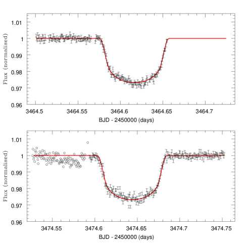
Figure 1: Our NTT/SUSI2 light curve for the first ($top$) and the second ($bottom$) observed transits of OGLE-TR-113b, with the best fit transit curve superimposed. For the second transit, the variations of the flux before the transit are due to a bad column of the CCD located close to the $PSF$ cores of OGLE-TR-113 and a bright reference star (open symbols).

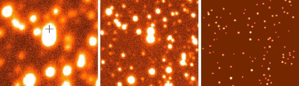
Figure 2: OGLE-TR-113 (marked with a cross) in a 256 pixels $\times$ 256 pixels sub-image (0.7 $\arcmin$ $\times$ 0.7 $\arcmin$) from the worst (left) and best (middle) seeing NTT/SUSI2 image of the run ($top$ = North, $left$ = East). The nearby star just South of OGLE-TR-113 is about 0.4 mag brighter. Right: deconvolved image. At this resolution (2 pixels = 0.32$\arcsec$), no trace of other faint companions is visible.

4.2 Transit fitting

The transit fitting was performed with transit curves computed with the procedure of Mandel & Agol (Mandel1 (2002)), using quadratic limb-darkening coefficients. The transit parameters were obtained in two iterations. A preliminary solution was first fitted to determine epochs for NTT photometric series. A period was then determined by comparing these epochs with OGLE-III ephemeris (Konacki et al. (2004)), allowing a very high accuracy on the period due to the large time interval separating the two sets of measurements (795 times the orbital period). The period was then fixed to this value and the radius ratio, orbital inclination, transit duration and transit epoch were fitted by least squares using the NTT data. The limb-darkening coefficients used were $u_{1}$ = 0.55 and $u_{2}$ = 0.18, obtained from Claret (2000) for the following stellar parameters: effective temperature $T_{eff}$ = 4750 K, metallicity $[M/H]$ = 0.1, surface gravity log $g$ = 4.5 and microturbulence velocity $\xi_{t}$ = 1.0 km/s, based on the parameters presented in Santos et al. (2006).

To obtain realistic uncertainties for the fitted transit parameters, it is essential to take into account the correlated noise present in the light curves, as shown by Pont et al. (2006, in prep. ). Although we have attained a very good level of stability in our photometry, the residuals are not entirely free of covariance at the sub-millimag level. We model the covariance of the noise from the residuals of the light curve itself. We estimate the amplitude of systematic trends in the photometry from the standard deviation over one residual point, $\sigma_{1}$ , and from the standard deviation of the sliding average of the residuals over 10 successive points, $\sigma_{10}$. The amplitude of the white noise $\sigma_{w}$ and the red noise $\sigma_{r}$ can then be obtained by resolution of the following system of 2 equations:

$$\sigma_{1}^{2} = \sigma_{w}^{2}+\sigma_{r}^{2}$$ (5)

$$\sigma_{10}^{2} = \frac{\sigma_{w}^{2}}{10}+\sigma_{r}^{2}$$ (6)

We obtained $\sigma_{r}$ = 400 $\mu$mag for both nights. We assume that a systematic feature of this amplitude could be present in the data over a length similar to the transit duration. Therefore, if $\chi_{bf}$ is the $\chi^{2}$ of the best fit, instead of using $\Delta\chi^{2}$ = 1 to define the 1-sigma uncertainty interval, we use

$$\Delta\chi^{2}=1+N_{tr,i}\frac{\sigma_{r,i}^{2}}{\sigma_{w,i}^{2}}$$ (7)

for each individual transit, where $N_{tr,i}$ is the number of points in the transit $i$. As the residuals between different transits are not correlated, combining the data from both individual transits gives:

$$\Delta\chi^{2}=\sqrt{\Delta\chi_{1}^{2}+\Delta\chi_{2}^{2}}$$ (8)

Exploring the parameters space for $\chi^{2}=$ $\chi^{2}_{bf}+\Delta\chi^{2}$, we then estimated the uncertainties on our parameters.

The results are given in Table 1. The fit of the final light curve on the NTT data is shown in Fig. 3. This figure also shows the final transit curve superimposed on the OGLE-III data (the limb-darkening coefficients are changed, as OGLE-III observations have been obtained in the $I$ filter), and the phased NTT/SUSI2 data after binning on 2 points superimposed on the best-fit transit curve. For this binned light curve, the dispersion before the transit is $\sim$800 $\mu$mag (first night), and $\sim$850 $\mu$mag after the transit (second night).

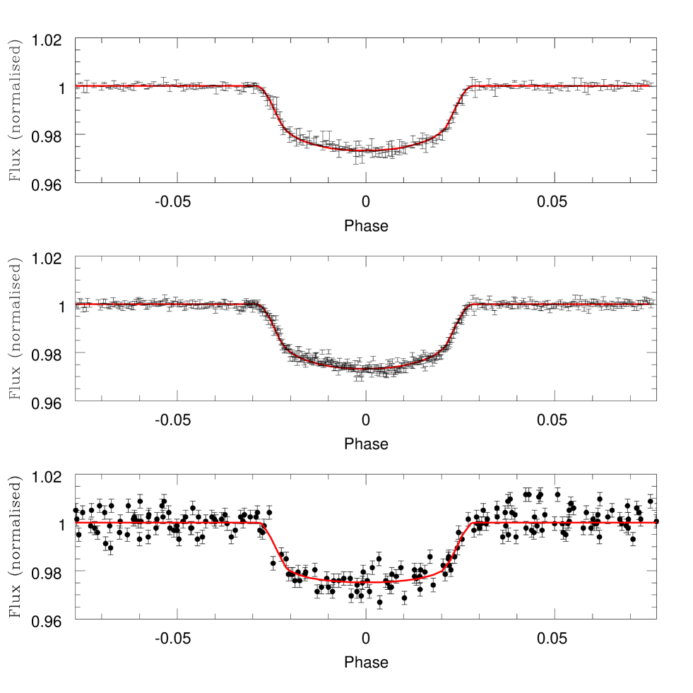
Figure 3: The best-fit transit curve is shown together with the phased NTT/SUSI2 data after binning on 2 points (top), without binning (middle) and with the phased OGLE-III data (bottom).

4.3 Radius and mass determination

Combining the constraints from our new transit curves (dependence on $R_{\ast}M_{\ast}^{-1/3}$) and from the spectroscopic determination of $T_{eff}$, log $g$ and [Fe/H] (Santos et al. (2006)), we computed the radius and mass of OGLE-TR-113 as in Bouchy et al. (2005), taking the relation between $M_{\ast}$, $R_{\ast}$, and the atmospheric parameters from an interpolation of Girardi et al. (Girardi1 (2002)) stellar evolution models. The value of the planetary radius was then derived from the radius ratio and from $R_{\ast}$. Next, we fitted a sinusoidal orbit by least–squares to the radial velocity data with the new period and epoch, obtaining the planetary mass from $M_{\ast}$ and the semi-amplitude of the radial velocity orbit.

Our values for the radius and mass of OGLE-TR-113 and its planetary companion are given in Table 1, which also presents the values obtained by Bouchy et al. (2004) and Konacki et al. (2004). Our results are in good agreement with the previous studies, but the uncertainties on the mass and on the radius of the planet are significantly lower. In fact, our high photometric accuracy allows to reach the regime where the uncertainties on the mass and radius of the primary dominate: the use of other stellar evolution models should introduce parameter changes which are of the same order than the error bars. The development of this point is beyond the scope of this paper.

	A	B	C
Inclination angle[deg]	$88.8-90$	85 - 90	$88.4\pm 2.2$
Period[days]	$1.4324757\pm 0.0000013$	$1.43250$ (adopted)	$1.4324758\pm 0.0000046$
Semi-major axis[AU]	$0.0229\pm 0.0002$	$0.0228\pm 0.0006$	$0.02299\pm 0.00058$
Eccentricity (fixed)	$0$	0	0
Primary mass[$M_{\odot}$]	$0.78\pm 0.02$	$0.77\pm 0.06$	$0.79\pm 0.06$ (adopted)
Primary radius[$R_{\odot}$]	$0.77\pm 0.02$	$0.765\pm 0.025$	$0.78\pm 0.06$ (adopted)
Planet mass[$M_{J}$]	$1.32\pm 0.19$	$1.35\pm 0.22$	$1.08\pm 0.28$
Planet radius[$R_{J}$]	$1.09\pm 0.03$	$1.08^{+0.07}_{-0.05}$	$1.09\pm 0.10$
Planet density[g cm-3]	$1.3\pm 0.3$	$1.3\pm 0.3$	$1.0\pm 0.4$

Table 1: Parameters obtained from this analysis (A) for OGLE-TR-113 and its planetary companion, compared to the ones presented in Bouchy et al. (2004) (B) and in Konacki et al. (2004) (C).

$T_{0,OGLE}$[BJD]	$2452325.79823\pm 0.00082$
$T_{0,1}$[BJD]	$2453464.61665\pm 0.00010$
$T_{0,2}$[BJD]	$2453474.64348\pm 0.00017$

Table 2: Ephemeris of OGLE-TR-113b transits. $T_{0,OGLE}$ is from Konacki et al. (2004), while $T_{0,1}$ and $T_{0,2}$ are for the two transits analyzed in this work.

4.4 Transit timing

OGLE-III (Konacki et al. (2004)) and our new NTT transits ephemeris are presented in Table 2. Using these ephemeris and assuming the absence of long-term transit period variations due, e.g., to the oblateness of the star or dissipative tidal interactions between the planet and the star, we obtained a value for the period in perfect agreement with the one presented in Konacki et al. (2004), but with a much smaller error bar. Our extremely high accuracy on the orbital period ($\sim$ 0.1 s) is mainly due to the long delay between OGLE-III and NTT observations. Moreover, our accuracy on the epoch of the NTT transits is $\sim$ 12 s, while the accuracy on the OGLE-III epoch is $\sim$ 71 s.

Short-term transit timing variations ($TTV$) may be induced by the presence of a satellite (Sartoretti & Schneider (1999)) or a second planet (Miralda-Escudé (2002), Agol et al. (2005), Holman & Murray (2005)). If we examine the temporal deviation of the second NTT transit off the expectation based on our period and the first NTT transit time, we obtain a value of $\sim 43$ s. This $TTV$ has a statistical significance of 2.5 sigmas. Nevertheless, we must stay cautious because systematics are able to slightly distort light curves, all the more so since these transit light curves are not complete. This is the case here: we lack the flat part after the first transit and, due to the bad column, the flat part prior to the second one. A way to estimate the likelihood of the hypothesis that systematics are responsible for the observed $TTV$ is to determine the transit ephemeris for the ingress and egress independently. Table 3 and Fig. 4 show the result. For both transits, transit times obtained from ingress and egress are in good agreement, leading us to reject such systematic errors as the explanation for the observed $TTV$.

$T_{0,1,ingress}$[BJD]	2453464.61669 $\pm$ 0.00014
$T_{0,1,egress}$[BJD]	2453464.61653 $\pm$ 0.00014
$T_{0,2,ingress}$[BJD]	2453474.64299 $\pm$ 0.00024
$T_{0,2,egress}$[BJD]	2453474.64400 $\pm$ 0.00024

Table 3: Ephemeris obtained from ingress and egress of both transits.

Figure 4: This figure shows the agreement between the transit times obtained from the complete light curves (top) and using ingress (I) and egress (E) independently (bottom) and the predicted transit times based on the determined period and OGLE-III ephemeris.

The statistical significance of the $TTV$ is rather low, as can be seen in Fig. 4. Future observations are needed to confirm its existence. We notice nevertheless that our timing accuracy would clearly be good enough to allow the detection of a third planet or a satellite giving rise to a $TTV$ amplitude of 1 minute. Considering the case of OGLE-TR-113b and, as the cause of such a $TTV$, a satellite with an orbital distance to the planet equal to the Hill radius, we can obtain an estimate of its mass by using the formula (Sartoretti & Schneider (1999)):

$$M_{s}\sim\pi\frac{\delta t}{P_{p}}\biggl{(}\frac{3M_{\ast}}{M_{p}}\biggr{)}^{1/3}M_{p}$$ (9)

where $M_{\ast}$, $M_{p}$ and $M_{s}$ are respectively the masses of the star, planet and satellite, $P_{p}$ is the orbital period of the planet and $\delta t$ the amplitude of the $TTV$. We obtain $M_{s}\sim 7M_{\oplus}$.

For an exterior pertubing planet, the most interesting case would be a pertubing planet in 2:1 mean–motion resonance with OGLE-TR-113b, for which we obtain with the following formula (Agol et al. (2005)):

$$M_{p2}=4.5\frac{\delta t}{P_{p1}}M_{p1}$$ (10)

a mass $\sim 1M_{\oplus}$.

These computations demonstrate the interest of high accuracy photometric follow-up of known transiting exoplanets and show that the accuracy obtained with our reduction method for high quality data would allow the detection of very low mass objects.

5 Conclusions

The results presented here show that our new photometry algorithm is well suited for follow-up transit photometry, even in very crowded fields. After analysis of NTT SUSI2 observations of two OGLE-TR-113b transits, we have obtained two very high accuracy transit light curves with a low level of systematic residuals. Combining our new photometric data with OGLE-III ephemeris, spectroscopic data and radial velocity measurements, we have determined planetary and stellar parameters in excellent agreement with the ones presented in Bouchy et al. (2004) and Konacki et al. (2004), but significantly more precise. We notice that the sampling in time, the sub-millimag photometric accuracy and the systematics residuals level of our light curves would be good enough to allow the photometric detection of a transiting Hot Neptune, in the case of a small star as OGLE-TR-113.

We have obtained a very precise determination of the transit times, and, combining them with OGLE-III ephemeris, we could determine the orbital period with a very high accuracy. The precisions on the epochs and the period would in fact be high enough to allow the detection of a second planet or a satellite, for some ranges of orbital parameters and masses. Even a terrestrial planet could be detected with such a transit timing precision.