Extended Curvaton reheating in inflationary models

Abstract

The curvaton reheating in a non-oscillatory inflationary universe model is studied in a Jordan-Brans-Dicke theory. For different scenarios, the temperature of reheating is computed. The result tells us that the reheating temperature becomes practically independent of the Jordan-Brans-Dicke parameter $w$. This reheating temperature results to be quite different when compared with that obtained from Einstein‘s theory of gravity.

I Introduction

It is well known that many long-standing problems of the Big Bang model (horizon, flatness, monopoles, etc.) may find a natural solution in the framework of the inflationary universe model guth ; infla .

One of the successes of the inflationary universe model is that it provides a causal interpretation of the origin of the observed anisotropy of the cosmic microwave background (CMB) radiation, and also the distribution of large scale structures astros . In standard inflationary universe models, the acceleration of the expansion of the universe is driven by a scalar field $\psi$ (inflaton) with a specific scalar potential, and the quantum fluctuations associated with this field generate the density perturbations seeding the structure formation at late time in the evolution of the universe. To date, the accumulating observational data, especially those coming from the CMB observations of the WMAP satellite astros , indicate that the power spectrum of the primordial density perturbations becomes nearly scale-invariant, just as predicted by the single-field inflationary model .

At the end of inflation the universe is typically in a highly non-thermal state. An exception is the warm inflation scenario, where there is particle production during inflation berera . The key ability of inflation is to homogenize the universe, which means that it leaves the universe at very low temperature and hence any successful theory of inflation must also explain how the universe was reheated - or perhaps defrosted - to the Big Bang picture Lyth1 . This approach must include baryogenesis and nucleosynthesis, the latter implying that the temperature must have been higher than 1 MeV and the former requiring energies significantly higher.

One path to defrost the universe after inflation is known as reheating Kolb1 . Elementary theory of reheating was developed in Dolgov for the new inflationary scenario. During reheating, most of the matter and radiation of the universe are created, usually via the decay of the scalar field that drives inflation, while the temperature grows in many orders of magnitude. Of particular interest is a quantity known as the reheating temperature. The reheating temperature is associated with the temperature of the universe when the Big Bang scenario begins, that is, when the radiation epoch begins. In general, this epoch is generated by the decay of the inflaton field, which leads to a creation of particles of different kinds.

The stage of oscillations of the scalar field is an essential part of the standard mechanism of reheating. However, there are some models where the inflaton potential does not have a minimum and the scalar field does not oscillate. Here, the standard mechanism of reheating does not work Kofman . These models are known in the literature as non-oscillating models, or simply NO models fengli ; Felder1 . The NO models correspond to runaway fields such as moduli fields in string theory which are potentially useful for inflation model-building because they present flat directions which survive the famous $\eta$-problem of inflation dine . On the other hand, an important use of NO models is quintessential inflation, in which the tail of the potential can be responsible for the accelerated expansion of the present universe Dimopoulus .

However, these models present another type of $\eta$-problem, which has to do with the fact that between the inflationary plateau and the quintessential tail there is a difference of over a hundred orders of magnitude. According to the above, it is useful to consider an exponential potentialDimopoulus . During inflation, the power law expansion may be realized if the inflaton field with an exponential potential dominates the energy density of the universe. Originally, this model was described in terms of Einstein‘s theory of gravity in Ref.Lucchin . However, during the past decade, a great number of studies based on a less standard theory have been carried out, namely, the Jordan-Brans-Dicke (JBD) theory Jbd .

JBD theory is characterized by the presence of a dynamic massless scalar field (the JBD field) which couples directly with the metric in the gravitational sector, providing a variable gravitational constant. The theory explicitly presents a nonminimal coupling between the scalar JBD field and the scalar curvature. In Ref.Susperregi is given a detailed discussion about inflation in the context of a JBD theory, for an exponential potential.

The first mechanism of reheating for NO models in general relativity theory was the gravitational particle production ford , but this mechanism is quite inefficient, since it may lead to certain cosmological problems ure a ; Sami_taq . An alternative mechanism of reheating in NO models is the instant preheating, which introduces an interaction between the scalar field responsible for inflation with another scalar field Felder1 . Another possibility for reheating in NO models is the introduction of the curvaton field, $\sigma$ ref1u , which has recently received a lot of attention in the literature L1 ; L2 . The curvaton approach is an interesting new proposal for explaining the observed large-scale adiabatic density perturbations in the context of inflation. Here, the hypothesis is such that the adiabatic density perturbation is originated from the “curvaton field” and not from the inflaton field. In this scenario, the adiabatic density perturbation is generated only after inflation, from an initial condition which corresponds to a purely isocurvature perturbation Mollerach .

On the other hand, the decay of the curvaton field into conventional matter offers an efficient mechanism of reheating. The curvaton field has the property that its energy density is not diluted during inflation, so that the curvaton may be responsible for some or all of the matter content of the universe at present.

In this paper we shall explore an application of curvaton reheating in a JBD theory for a NO model. Specifically we explore the model to an exponential scalar potential.

We follow a similar procedure described in Refs.ure a ; cdh1 ; cdh2 . As the energy density decreases, the inflaton field makes a transition into a kinetic energy dominated regime bringing inflation to an end. We consider the evolution of the curvaton field through three different stages. Firstly, there is a period in which the inflaton energy density is the dominant component, i.e, $\rho_{\psi}\gg\rho_{\sigma}$, even though the curvaton field survives the rapid expansion of the universe. The following stage i.e., during the kinetic epoch refere3 , is that in which the curvaton mass becomes important. In order to prevent a period of curvaton-driven inflation, the universe must remain inflaton-driven until this time. When the effective mass of the curvaton becomes important, the curvaton field starts to oscillate around the minimum of its potential. The energy density, associated with the curvaton field, starts to evolve as non-relativistic matter.

At the final stage, the curvaton field decays into radiation and then the standard Big Bang cosmology is recovered afterwards. In general, the decay of the curvaton field should occur before nucleosynthesis happens. Other constraints may arise depending on the epoch of the decay, which is governed by the decay parameter, $\Gamma_{\sigma}$. There are two scenarios to be considered, depending on whether the curvaton field decays before or after it becomes the dominant component of the universe.

In section II the inflationary dynamics in a JBD theory is described. In section III the dynamics of the extended model in the kinetic epoch is developed. Section IV studies the dynamics of the curvaton field through different stages. In section V some constraints from gravitational waves in the kinetic epoch are described. Finally we present the conclusions section VI.

II Extended Inflationary Model

The dynamics of the Friedman-Robertson-Walker cosmology in the JBD theory, is described by the equations

$$\ddot{\Phi}+3H\dot{\Phi}=\frac{8\pi}{(2w+3)}(\rho_{\psi}-3P_{\psi})\;,$$ (1)

$$H^{2}\,+H\frac{\dot{\Phi}}{\Phi}=\frac{8\pi}{3}\frac{1}{\Phi}\rho_{\psi}+\frac{w}{6}\left(\frac{\dot{\Phi}}{\Phi}\right)^{2},$$ (2)

and

$$\ddot{\psi}+3H\dot{\psi}=-\frac{\partial V(\psi)}{\partial\psi},$$ (3)

where $\Phi$ denotes the JBD scalar field (with unit $m_{p}^{2}$, where $m_{p}$ is the Planck mass), $H=\dot{a}/a$ is the Hubble factor, $a$ is a scale factor, $\psi$ the standard inflaton field, $V(\psi)$ is the effective potential associated with this field, and we assume to be

$$V(\psi)=V_{0}e^{-\alpha\psi},$$

where $\alpha$ and $V_{0}$ are free parameters. In the following we shall take $\alpha>0$ (with unit $1/m_{p}$). In Einstein‘s theory of gravity, power law inflation may take place if $\alpha<\sqrt{2}/m_{p}$Lucchin . Here, $P_{\psi}$ represents the pressure associated with the infaton field, and $w=Constant$ corresponds to the JBD parameter. As is mentioned in Ref.omega , experimental tests of weak-field in the solar-system have constrained the post-Newtonian deviation from Einstein gravity, where it was found that the JBD parameter should satisfy the inequality $w>500$. According to recent reports, this bound would increase to several thousands omega121314 . Moreover, the Einstein‘s theory of gravity is recovered in the limits $w\longrightarrow\infty$ and $\Phi=Cte.=m_{p}^{2}$. Dots mean derivatives with respect to time and we use units in which $c=\hbar=1$.

During inflation the $\ddot{\Phi}$ term in Eq.(1) can be ignored in the sense that $\ddot{\Phi}\ll H\dot{\Phi}$. Also, $\dot{\Phi}/\Phi\ll H$ (because $w\gg 1$) and $\rho_{\psi}\sim V(\psi)$, since $\dot{\psi}^{2}/2<V(\psi)$. Under this approximation the field equations (1) and (2) become,

$$3H\dot{\Phi} = \frac{32\pi}{2w+3}V,$$ (4)

$$H^{2} = \frac{8\pi}{3}\frac{V}{\Phi}.$$ (5)

Now, from Eq.(3) we get, under the slow roll approximation for the inflaton field $\psi$ ($\ddot{\psi}$ is negligible)

$$3H\dot{\psi}=-\frac{\partial V}{\partial\psi},$$ (6)

and combining the Eqs. (4) and (5) we have,

$$\frac{\dot{\Phi}}{\Phi}=\frac{4H}{2w+3},$$ (7)

which gives

$$\frac{\Phi}{\Phi_{i}}=\left(\frac{a}{a_{i}}\right)^{\beta},$$ (8)

where $\beta=4/(2w+3)$. We see that the JBD field $\Phi$ increases during the inflationary epoch. Now, from Eqs. (5), (6) and (8), we get

$$\frac{\psi}{\psi_{i}}=\left(\frac{a}{a_{i}}\right)^{\beta}=\frac{\Phi}{\Phi_{i}},$$ (9)

where we have chosen the initial condition $\Phi_{i}=8\pi\psi_{i}\beta/\alpha$.

During the inflationary epoch we could write $H_{i}^{2}=H_{f}^{2}\frac{\Phi_{f}V_{i}}{\Phi_{i}V_{f}}=H_{f}^{2}\frac{\Phi_{f}}{\Phi_{i}}e^{-\alpha(\psi_{i}-\psi_{f})}$, where the subscripts $i$ and $f$ are used to denote the beginning and the end of inflation, respectively. Inflation ends when the slow roll condition, is not satisfied anymore, i.e.

$$\epsilon_{f}=-\frac{\dot{H}}{H^{2}}=\left[\frac{2}{(3+2w)}+\frac{\Phi}{16\pi}\left(\frac{V_{,\psi}}{V}\right)^{2}\right]_{f}\simeq 1,$$

from which we get that $\Phi_{f}=\frac{16\pi}{\alpha^{2}}(1-\beta/2)=\frac{8\pi\beta}{\alpha}\psi_{f}>0$, i.e. $\beta$ is less than 2. There, we have denoted $V,_{\psi}=\partial V/\partial\psi$. The initial value of the square Hubble factor as a function of the total number of e-foldings, $N_{0}=\ln(a_{f}/a_{i})$, becomes

$$H_{i}^{2}=\frac{\alpha^{2}V_{0}}{3(2-\beta)}e^{(N_{0}\beta-\alpha\psi_{i})}.$$ (10)

III Kinetic Epoch

When inflation has finished, the term $\partial V/\partial\psi$ is negligible compared to the friction term. This epoch is called the ‘kinetic epoch’ or ‘kination’ refere3 , and we will use the subscript ‘k’ to label the values of the different quantities at the beginning of this epoch. The kinetic epoch does not occur immediately after inflation; there may exist a middle epoch where the potential force is negligible with respect to the friction term Guo . In the kinetic epoch we have $\dot{\psi}^{2}/2>V(\psi)$ corresponding to the relation $P_{\psi}=\rho_{\psi}$ which represents a stiff fluid.

The dynamics of the Friedman-Robertson-Walker cosmology in the JBD theory, in the kinetic epoch, is described by the equations

$$\ddot{\Phi}+3H\dot{\Phi}=-\frac{8\pi}{(2w+3)}\;\dot{\psi}^{2},$$ (11)

$$H^{2}\,+H\frac{\dot{\Phi}}{\Phi}=\frac{8\pi}{3}\frac{1}{\Phi}\frac{\dot{\psi}^{2}}{2}+\frac{w}{6}\left(\frac{\dot{\Phi}}{\Phi}\right)^{2},$$ (12)

and

$$\ddot{\psi}+3H\dot{\psi}=0\Longrightarrow\;\dot{\psi}=\frac{\dot{\psi}_{k}a_{k}^{3}}{a^{3}}.$$ (13)

The energy density of the inflaton field is defined by $\rho_{\psi}=\dot{\psi}^{2}/2+V(\psi)\simeq\dot{\psi}^{2}/2$ and, since it has a behavior like stiff matter, we get that $\rho_{\psi}\propto(1/a)^{6}$.

From Eqs.(11) and (13), we have

$$\ddot{\Phi}+3H\dot{\Phi}=-\frac{8\pi}{(2w+3)}\;\frac{\dot{\psi}_{k}^{2}a_{k}^{6}}{a^{6}}.$$ (14)

If we introduce a new variable, $dt=a^{3}d\eta$, Eq.(14) is solved and gives Barrow

$$\Phi=\Phi_{k}-\frac{4\pi}{(2w+3)}\dot{\psi_{k}}^{2}a_{k}^{6}(\eta-\eta_{k})^{2},$$ (15)

where we have chosen the initial conditions $\left.\frac{d\Phi}{d\eta}\right|_{\eta=\eta_{k}}=\left.\Phi^{\prime}\right|_{\eta=\eta_{k}}=\Phi^{\prime}_{k}=0$. We note that, during the kinetic epoch , $\Phi^{\prime}<0$ as it could be seen from Eq.(15). In this period the JBD field, $\Phi(\eta)$, is greater than the value $\Phi_{0}=\frac{1}{G}=m_{p}^{2}$. In this way the JBD field lies in the range $\Phi_{k}>\Phi(\eta)>\Phi_{0}$, where $\Phi_{0}$ is the actual value of the JBD field and $G$ is the Newton constant.

Using the solutions given by Eqs. (13) and (15), we may write

$$\rho_{\psi}=\rho_{\psi}^{k}\frac{a_{k}^{6}}{a^{6}},$$ (16)

and

$$H(a,\Phi)=H=H_{k}\frac{a_{k}^{3}}{a^{3}}\left[\frac{\sqrt{\Phi_{k}}}{\sqrt{1+2w/3}}\left(\frac{\sqrt{(\Phi_{k}-\Phi)}}{\Phi}+\sqrt{\Phi_{k}\left[1+\frac{2w}{3}\right]}\;\;\frac{1}{\Phi}\right)\right].$$ (17)

Note that, in the limit $w\longrightarrow\infty$ and $\Phi=Cte.=\Phi_{k}=m_{p}^{2}$, we obtained the Hubble factor in the GR theory which follows the law $H^{(GR)}\propto(1/a)^{3}$.

IV Curvaton Field

We now study the dynamics of the curvaton field, $\sigma$, through different stages. This study allows us to find some constraints on the parameters and thus, to have a viable curvaton scenario. We considered that the curvaton field obeys the Klein-Gordon equation and, for simplicity, we assume that its scalar potential associated with this field is given by

$$U(\sigma)=\frac{m^{2}\sigma^{2}}{2}\;,$$ (18)

where $m$ is the curvaton mass.

First of all, it is assumed that the energy density $\rho_{\psi}$, associated with the inflaton field, is the dominant component when it is compared with the curvaton energy density, $\rho_{\sigma}$. In the next stage, the curvaton field oscillates around the minimum of the effective potential $U(\sigma)$. Its energy density evolves as a non-relativistic matter and, during the kinetic epoch, the universe remains inflaton-dominated. The latter stage corresponds to the decay of the curvaton field into radiation and then the standard Big-Bang cosmology is recovered.

In the inflationary regime it is supposed that the curvaton field is effectively massless and its dynamics is described in detail in Refs.dimo ; postma ; ure a . During inflation, the curvaton would roll down its potential until its kinetic energy is depleted by the exponential expansion and only then, i.e. only after its kinetic energy has almost vanished, it becomes frozen and assumes roughly a constant value, i.e. $\sigma_{*}\approx\sigma_{f}$. The subscript $``*^{\prime\prime}$ here refers to the epoch when the cosmological scales exit the horizon.

The hypothesis is that during the kinetic epoch the Hubble parameter decreases so that its value is comparable with the curvaton mass, i.e. $m\simeq H$ (the curvaton field becomes effectively massive). From Eq.(17), we obtain

$$\frac{m}{H_{k}}=\frac{a_{k}^{3}}{a_{m}^{3}}\left[\frac{\sqrt{\Phi_{k}}}{\sqrt{1+2w/3}}\;\;\frac{1}{\Phi_{m}}\left(\sqrt{(\Phi_{k}-\Phi_{m})}+\sqrt{\Phi_{k}\left[1+\frac{2w}{3}\right]}\;\;\right)\right],$$ (19)

where the ‘m’ label represents the quantities at the time when the curvaton mass is of the order of $H$ during the kinetic epoch.

In order to prevent a period of curvaton-driven inflation, the universe must still be dominated by the inflaton matter, i.e. $\rho_{\psi}|_{a_{m}}=\rho_{\psi}^{(m)}\gg\rho_{\sigma}(\sim\,U(\sigma_{f})\simeq\,U(\sigma_{*}))$ . This inequality allows us to find a constraint on the values of the curvaton field $\sigma_{*}$ in the epoch when the cosmological scales exit the horizon. Then, from Eq.(12) at the moment when $H\simeq m$, we obtain the inequality

$$\frac{m^{2}\sigma_{*}^{2}}{2\rho_{\psi}^{(m)}}\ll 1\Rightarrow\sigma_{*}^{2}\ll\frac{3\Phi_{m}}{4\pi}\left[1+\frac{1}{m}\left(\frac{\dot{\Phi}}{\Phi}\right)_{m}-\frac{w}{6\;m^{2}}\left(\frac{\dot{\Phi}}{\Phi}\right)_{m}^{2}\right],$$ (20)

in which

$$\left(\frac{\dot{\Phi}}{\Phi}\right)_{m}=-2H_{k}\left(\frac{a_{k}}{a_{m}}\right)^{3}\frac{1}{\sqrt{1+2w/3}}\frac{\Phi_{k}}{\Phi_{m}}\frac{\sqrt{\Phi_{k}-\Phi_{m}}}{\sqrt{\Phi_{k}}},$$ (21)

where the last expression is obtained by using Eq.(15).

The value given by Eq.(20), coincides with that found in general relativity theory, which is obtained by taking the limit $\Phi=Cte.=\Phi_{k}=\Phi_{m}=m_{p}^{2}$ and $w\rightarrow\infty$ ure a .

The ratio between the potential energies at the end of inflation is given by

$$\frac{U_{f}}{V_{f}}=\frac{4\pi}{3}\frac{m^{2}\sigma_{*}^{2}}{\Phi_{f}\;H_{f}^{2}}\ll\frac{m^{2}\;\Phi_{m}}{H_{f}^{2}\;\Phi_{f}}\left[1+\frac{1}{m}\left(\frac{\dot{\Phi}}{\Phi}\right)_{m}-\frac{w}{6\;m^{2}}\left(\frac{\dot{\Phi}}{\Phi}\right)_{m}^{2}\right],$$ (22)

and, in this way, the curvaton energy becomes subdominant at the end of inflation or, equivalently

$$m^{2}\;\frac{\Phi_{m}}{\Phi_{f}}\left[1+\frac{1}{m}\left(\frac{\dot{\Phi}}{\Phi}\right)_{m}-\frac{w}{6\;m^{2}}\left(\frac{\dot{\Phi}}{\Phi}\right)_{m}^{2}\right]\ll H_{f}^{2}\;.$$ (23)

In these expressions, we have used $V_{f}=(3/8\pi)H_{f}^{2}\,\Phi_{f}$ and Eq.(20). Here, $\Phi_{f}$ is the value of the JBD field at the end of inflation. Note that $U_{f}\ll V_{f}$ as it could be seen from Eq.(22).

At the time when the mass of the curvaton field becomes important, i.e. $m\simeq H$, its energy decays like a non-relativistic matter in the form

$$\rho_{\sigma}=\frac{m^{2}\sigma_{*}^{2}}{2}\frac{a_{m}^{3}}{a^{3}}.$$ (24)

IV.1 Curvaton Decay After Domination

As we have claimed, the curvaton decay could occur in two different possible scenarios. In the first scenario, when the curvaton comes to dominate the cosmic expansion (i.e. $\rho_{\sigma}>\rho_{\psi}$), there must be a moment when the inflaton and curvaton energy densities become equal. From Eqs.(16), (17) and (24) at the time when $\rho_{\sigma}=\rho_{\psi}$, which happens when $a=a_{eq}$, we get

$$\left.\frac{\rho_{\sigma}}{\rho_{\psi}}\right|_{a=a_{eq}}=\frac{m^{2}\sigma_{*}^{2}}{2}\frac{a_{m}^{3}\;a_{eq}^{3}}{a_{k}^{6}\;\rho_{\psi}^{k}}=\frac{4\pi}{3}\frac{m^{2}\sigma_{*}^{2}a_{m}^{3}a_{eq}^{3}}{H_{k}^{2}\Phi_{k}a_{k}^{6}}=1,$$ (25)

where we have used $H_{k}^{2}=\frac{8\pi}{3\Phi_{k}}\rho_{\psi}^{k}$, since we have that $\dot{\Phi}_{k}=\Phi^{\prime}_{k}=0$.

Now from Eqs.(17), (19) and (25), we may write a relation for the Hubble parameter, $H(a_{eq})=H_{eq}$, in terms of curvaton parameters, the scale factor and the JBD scalar field

$$H_{eq} = H_{k}\frac{a_{k}^{3}}{a_{eq}^{3}}\left[\frac{\sqrt{\Phi_{k}}}{\sqrt{1+2w/3}}\;\frac{1}{\Phi_{eq}}\left(\sqrt{(\Phi_{k}-\Phi_{eq})}+\sqrt{\Phi_{k}\left[1+\frac{2w}{3}\right]}\;\right)\right]$$ (26)

$$= \frac{4\pi}{3}\frac{m\sigma_{*}^{2}}{(1+2w/3)}\frac{1}{\Phi_{m}\Phi_{eq}}\left(\sqrt{(\Phi_{k}-\Phi_{m})}+\sqrt{\Phi_{k}\left[1+\frac{2w}{3}\right]}\;\;\right)\left(\sqrt{(\Phi_{k}-\Phi_{eq})}+\sqrt{\Phi_{k}\left[1+\frac{2w}{3}\right]}\;\;\right).$$

This result should be compared to the corresponding result associated with the general relativity theory, where $H_{eq}^{(GR)}=4\pi\sigma_{*}^{2}m/3m_{p}^{2}$.

On the one hand, the decay parameter $\Gamma_{\sigma}$ is constrained by nucleosynthesis. For this, it is required that the curvaton field decays before nucleosynthesis, which means $H_{nucl}\sim 10^{-40}m_{p}<\Gamma_{\sigma}$. On the other hand, we also require that the curvaton decay occurs after $\rho_{\sigma}>\rho_{\psi}$, and $\Gamma_{\sigma}<H_{eq}$, so that we get a constraint on the decay parameter, which is given by

$$10^{-40}m_{p}<\Gamma_{\sigma}<\frac{4\pi m\sigma_{*}^{2}}{3(1+2w/3)}\frac{1}{\Phi_{m}\Phi_{eq}}\left(\sqrt{(\Phi_{k}-\Phi_{m})}+\sqrt{\Phi_{k}\left[1+\frac{2w}{3}\right]}\;\;\right)\left(\sqrt{(\Phi_{k}-\Phi_{eq})}+\sqrt{\Phi_{k}\left[1+\frac{2w}{3}\right]}\;\;\right),$$ (27)

which, in the particular case when $\Phi_{k}\simeq\Phi_{m}$, we obtain that $H_{eq}\simeq 4\pi\sigma_{*}^{2}m/3\Phi_{eq}\left(1+\frac{1}{\sqrt{1+2w/3}}\sqrt{\frac{\Phi_{k}-\Phi_{eq}}{\Phi_{k}}}\right)$. Furthermore, if we demand that $w\gg 1$ we find that $H_{eq}\simeq 4\pi\sigma_{*}^{2}m/3\Phi_{eq}=H_{eq}^{(GR)}m_{p}^{2}/\Phi_{eq}$ and therefore the decay parameter becomes constrained in the range $10^{-40}m_{p}<\Gamma_{\sigma}<4\pi\sigma_{*}^{2}m/3\Phi_{eq}$.

It is interesting to give an estimate of the constraint of the parameters of our model, by using the scalar perturbation related to the curvaton field. During the time where the fluctuations are inside the horizon, they obey the same differential equation as the inflaton fluctuations do, from which we conclude that they acquire the amplitude $\delta\sigma_{*}\simeq H_{*}/2\pi$. On the other hand, outside of the horizon, the fluctuations obey the same differential equation as the unperturbed curvaton field and then, we expect that they remain constant during inflation. The spectrum of the Bardeen parameter $P_{\zeta}$, whose observed value is about $2\times 10^{-9}$, allows us to determine the value of the curvaton field $\sigma_{*}$ in terms of the parameters $\alpha$, $w$ and the JBD scalar field. At the time when the decays of the curvaton fields occur, the Bardeen parameter becomes ref1u

$$P_{\zeta}\simeq\frac{1}{9\pi^{2}}\frac{H_{*}^{2}}{\sigma_{*}^{2}}.$$ (28)

The spectrum of fluctuations is automatically gaussian for $\sigma_{*}^{2}\gg H_{*}^{2}/4\pi^{2}$, and is independent of $\Gamma_{\sigma}$ ref1u . This feature will simplify the analysis in the space parameter of our model. Moreover, the spectrum of fluctuations is the same as in the standard scenario.

¿From expression (28) and by using that $H_{*}^{2}=H_{f}^{2}\Phi_{f}V_{*}/(\Phi_{*}V_{f})$, we relate the perturbations to the parameters of the model such that we get

$$V_{0}=27\pi^{2}(2-\beta)\frac{P_{\zeta}}{\alpha^{2}}\;\,\sigma_{*}^{2}\;e^{(\alpha\psi_{*}-N_{*}\beta)},$$ (29)

where $N_{*}=\ln(a_{f}/a_{*})$ is the number of the e-folds corresponding to the cosmological scales, i.e. the number of remaining inflationary e-folds at the time when the cosmological scale exits the horizon. The last expression allows us to fix the initial value of the effective potential in terms of the free parameters $\alpha$ and $w$. The constraint Eq. (23) in terms of $V_{0}$ becomes

$$m^{2}\left[1+\frac{1}{m}\left(\frac{\dot{\Phi}}{\Phi}\right)_{m}-\frac{w}{6\;m^{2}}\left(\frac{\dot{\Phi}}{\Phi}\right)_{m}^{2}\right]\ll\frac{8\pi}{3m_{p}^{2}\Phi_{m}}V_{0}e^{(1-2/\beta)}.$$ (30)

IV.2 Curvaton Decay Before Domination

For the second scenario, the decay of the field happens before this dominates the cosmological expansion. We need that the curvaton field decays before its energy density becomes greater than the inflaton one. Additionally, the mass of the curvaton is non-negligible, so that we could use Eq. (24). The curvaton decays at a time when $\Gamma_{\sigma}=H$ and then from Eq. (17) we get

$$\frac{\Gamma_{\sigma}}{H_{k}}=\frac{a_{k}^{3}}{a_{d}^{3}}\left[\frac{\sqrt{\Phi_{k}}}{\sqrt{1+2w/3}}\;\frac{1}{\Phi_{d}}\left(\sqrt{(\Phi_{k}-\Phi_{d})}+\sqrt{\Phi_{k}\left[1+\frac{2w}{3}\right]}\;\right)\right],$$ (31)

where ‘ d’ labels the different quantities at the time when the curvaton decays, allowing the curvaton field to decay after its mass becomes important, so that $\Gamma_{\sigma}<m$; and before the curvaton field dominates the expansion of the universe, i.e., $\Gamma_{\sigma}>H_{eq}$ (see Eq. (26)). Thus, we derive the new constraints on the decay parameter, given by

$$\frac{4\pi}{3}\frac{m\sigma_{*}^{2}}{(1+2w/3)}\frac{1}{\Phi_{m}\Phi_{eq}}\left(\sqrt{(\Phi_{k}-\Phi_{m})}+\sqrt{\Phi_{k}\left[1+\frac{2w}{3}\right]}\;\;\right)\left(\sqrt{(\Phi_{k}-\Phi_{eq})}+\sqrt{\Phi_{k}\left[1+\frac{2w}{3}\right]}\;\;\right)<\Gamma_{\sigma}<m.$$ (32)

Now, for the second scenario, the curvaton decays at the time when $\rho_{\sigma}<\rho_{\psi}$. If we define the $r_{d}$ parameter as the ratio between the curvaton and the inflaton energy densities, evaluated at $a=a_{d}$ and for $r_{d}\ll 1$, the Bardeen parameter is given by ref1u ; L1L2

$$P_{\zeta}\simeq\frac{r_{d}^{2}}{16\pi^{2}}\frac{H_{*}^{2}}{\sigma_{*}^{2}}.$$ (33)

With the help of Eqs. (19) and (31) we obtain

$$r_{d} = \left.\frac{\rho_{\sigma}}{\rho_{\psi}}\right|_{a=a_{d}}=\frac{4\pi}{3}\frac{m^{2}\sigma_{*}^{2}a_{m}^{3}a_{d}^{3}}{H_{k}^{2}\Phi_{k}a_{k}^{6}}=$$ (34)

$$= \frac{4\pi\sigma_{*}^{2}}{3}\frac{m}{\Gamma_{\sigma}}\frac{1}{(1+2w/3)}\frac{1}{\Phi_{m}\Phi_{d}}\left(\sqrt{(\Phi_{k}-\Phi_{m})}+\sqrt{\Phi_{k}\left[1+\frac{2w}{3}\right]}\;\;\right)\left(\sqrt{(\Phi_{k}-\Phi_{d})}+\sqrt{\Phi_{k}\left[1+\frac{2w}{3}\right]}\;\;\right).$$

Also, from Eq. (32) we get that

$$r_{d}<\frac{\Phi_{eq}}{\Phi_{d}}\frac{\left(\sqrt{(\Phi_{k}-\Phi_{d})}+\sqrt{\Phi_{k}\left[1+\frac{2w}{3}\right]}\;\;\right)}{\left(\sqrt{(\Phi_{k}-\Phi_{eq})}+\sqrt{\Phi_{k}\left[1+\frac{2w}{3}\right]}\;\;\right)},$$

then, from $r_{d}\ll 1$, the last expression is written

$$\frac{\Phi_{eq}}{\left(\sqrt{(\Phi_{k}-\Phi_{eq})}+\sqrt{\Phi_{k}\left[1+\frac{2w}{3}\right]}\;\;\right)}\ll\frac{\Phi_{d}}{\left(\sqrt{(\Phi_{k}-\Phi_{d})}+\sqrt{\Phi_{k}\left[1+\frac{2w}{3}\right]}\;\;\right)},$$

allowing us to use expression (33) for the Bardeen parameter.

Expressions (33) and (34) could be written

$$\sigma_{*}^{2}=9\frac{P_{\zeta}}{m^{2}}\frac{\Gamma_{\sigma}^{2}}{H_{*}^{2}}(1+2w/3)^{2}\frac{\Phi_{m}^{2}}{\left(\sqrt{(\Phi_{k}-\Phi_{m})}+\sqrt{\Phi_{k}\left[1+\frac{2w}{3}\right]}\;\;\right)^{2}}\frac{\Phi_{d}^{2}}{\left(\sqrt{(\Phi_{k}-\Phi_{d})}+\sqrt{\Phi_{k}\left[1+\frac{2w}{3}\right]}\;\;\right)^{2}},$$ (35)

and thus, expression (32) becomes

$$12\pi\frac{\Phi_{m}\Phi_{d}^{2}}{\Phi_{eq}}\frac{\left(1+\frac{2w}{3}\right)}{\left(\sqrt{(\Phi_{k}-\Phi_{d})}+\sqrt{\Phi_{k}\left[1+\frac{2w}{3}\right]}\;\;\right)^{2}}\frac{\left(\sqrt{(\Phi_{k}-\Phi_{eq})}+\sqrt{\Phi_{k}\left[1+\frac{2w}{3}\right]}\;\;\right)}{\left(\sqrt{(\Phi_{k}-\Phi_{m})}+\sqrt{\Phi_{k}\left[1+\frac{2w}{3}\right]}\;\;\right)}\;\frac{P_{\zeta}}{m^{2}H_{*}^{2}}\;\Gamma_{\sigma}^{2}<\frac{\Gamma_{\sigma}}{m}<1.$$ (36)

The upper limit for the $\Gamma_{\sigma}$ parameter, results to be

$$\Gamma_{\sigma}<\frac{mH_{*}^{2}\Phi_{eq}}{12\pi\Phi_{m}\Phi_{d}^{2}P_{\zeta}}\frac{(\sqrt{\Phi_{k}-\Phi_{d}}+\sqrt{\Phi_{k}(1+2w/3)})^{2}(\sqrt{\Phi_{k}-\Phi_{m}}+\sqrt{\Phi_{k}(1+2w/3)})}{(1+2w/3)(\sqrt{\Phi_{k}-\Phi_{eq}}+\sqrt{\Phi_{k}(1+2w/3)})}.$$ (37)

In the limit $w\rightarrow\infty$ and $\Phi_{eq}=\Phi_{d}=\Phi_{m}=\Phi_{0}=1/G=m_{p}^{2}$ the last expression gives $\Gamma_{\sigma}<(12\pi P_{\zeta})^{-1}mH_{*}^{2}G$, which corresponds to the result obtained in the Einstein theory of general relativity ure a . Also, we see that $\Gamma_{\sigma}<\left.\frac{m\Phi_{k}\Phi_{eq}H_{*}^{2}}{12\pi P_{\zeta}\Phi_{m}\Phi_{d}^{2}}\right|_{w\gg 1}$. This tells us that, for $w\gg 1$, the upper limit for the $\Gamma_{\sigma}$ parameter depends on the values of the JBD scalar field evaluated at the different epochs.

V Constraints from gravitational waves

The study of gravitational waves that can be applied to our model was described in Ref.Staro1 . It is interesting to give an estimate of the constraint on the curvaton mass, using this type of tensorial perturbation. Under the approximation give in Ref.Staro2 , the corresponding gravitational wave amplitude in the model by using JBD theory may be written as

$$h_{GW}\simeq\,C_{1}\,H_{*}.$$

According to Ref. Dimo we could have that $H\ll 10^{-5}m_{p}$ and $C_{1}$ is an arbitrary constant with unit of $1/m_{p}$. This interesting thing comes from the fact that inflation could take place at an energy scale smaller than grand unification. We note this as an advantage of the curvaton approach against of the single inflaton field scenario.

Now, using $H^{2}_{*}=H_{f}^{2}\frac{\Phi_{f}}{\Phi_{*}}e^{-\alpha(\psi_{*}-\psi_{f})}$, we obtain

$$h_{GW}^{2}\simeq\,C_{1}^{2}H_{f}^{2}\left(\frac{\Phi_{f}}{\Phi_{*}}\right)\;e^{-\alpha(\psi_{*}-\psi_{f})}.$$ (38)

In this way, from Eqs.(23) and (38) we derive the inequality

$$m^{2}\left[1+\frac{1}{m}\left(\frac{\dot{\Phi}}{\Phi}\right)_{m}-\frac{w}{6\;m^{2}}\left(\frac{\dot{\Phi}}{\Phi}\right)_{m}^{2}\right]\ll\,\frac{\Phi_{*}}{\Phi_{m}}\,\frac{h_{GW}^{2}}{C_{1}^{2}}\,e^{\alpha(1/\alpha+\beta\alpha\Phi_{*}/8\pi)},$$ (39)

and, in the particular case when $\Phi_{k}\simeq\Phi_{m}\simeq\Phi_{*}$, from Eq. (21) we see that $(\dot{\Phi}/\Phi)_{m}\simeq 0$ and, observing that Eq. (39) gives the following inequality: $m^{2}\ll\,\frac{h_{GW}^{2}}{C_{1}^{2}}\,e^{\alpha(1/\alpha+\beta\alpha m_{p}^{2}/8\pi)}$.

We note that we have $V_{,\psi\psi}=3\alpha^{2}\Phi_{f}H_{f}^{2}/8\pi$ and, if according to Ref. Dimo , if the inflaton field is effectively massless, then its contribution to the curvature perturbation will not be negligible and, in fact, could be in excess related to the observational limit from COBE. This can be avoided if the inflaton is massive, i.e. $V_{,\psi\psi}>H_{f}^{2}$ or equivalently $\alpha^{2}>8\pi/3\Phi_{f}$, in which case its perturbations are exponentially suppressed as it could be seen from this inequality.

In order to give an estimate of the gravitational wave, we move to the kinetic epoch in which the energy density of gravitational waves evolves as in Refs.Dimopoulus ; referee4 :

$$\rho_{g}=\frac{32}{3\pi}h_{GW}^{2}\rho_{\psi}\left(\frac{a}{a_{k}}\right)^{2}.$$ (40)

On the other hand, when the curvaton field decays, i.e. ($\Gamma_{\sigma}\sim H$), it produces radiation which decays as $1/a^{4}$. Then, when the curvaton decays, we may write for the energy density

$$\rho_{r}^{(\sigma)}=\frac{m^{2}\sigma_{*}^{2}}{2}\frac{a_{m}^{3}}{a_{d}^{3}}\frac{a_{d}^{4}}{a^{4}}.$$ (41)

In order to keep the gravitational waves under control, we assume that the radiation energy density is much larger than that produced by inflation ure a . Thus, at a time when $a=a_{eq}$, we write

$$\left.\frac{\rho_{r}^{(\sigma)}}{\rho_{\psi}}\right|_{a=a_{eq}}=\frac{4\pi}{3\Phi_{k}}\frac{m^{2}\sigma_{*}^{2}}{H_{k}^{2}}\frac{a_{m}^{3}}{a_{k}^{3}}\frac{a_{eq}^{2}}{a_{k}^{2}}\frac{a_{d}}{a_{k}}=1.$$ (42)

Therefore, the constraint from the gravitational waves now reads

$$\left.\frac{\rho_{g}}{\rho^{(\sigma)}_{r}}\right|_{a=a_{eq}}=\frac{64}{3\pi}h_{GW}^{2}\left(\frac{a_{eq}}{a_{k}}\right)^{2}$$

$$\hskip 42.67912pt=\frac{16}{\pi^{2}}h_{GW}^{2}\frac{H_{k}}{m\sigma_{*}^{2}}\left(\frac{\Gamma_{\sigma}}{H_{k}}\right)^{1/3}\frac{\Phi_{m}\Phi_{d}^{1/3}\Phi_{k}^{1/3}}{[\sqrt{(\Phi_{k}-\Phi_{m})}+\sqrt{\Phi_{k}(1+2w/3)}]}\frac{(1+2w/3)^{2/3}}{[\sqrt{(\Phi_{k}-\Phi_{d})}+\sqrt{\Phi_{k}(1+2w/3)}]^{1/3}}\ll 10^{-6},$$ (43)

where we have used Eqs.(19), (31) and (42).

We note that from Eq. (43) we obtain a bound for the mass of the curvaton, $m$, given by

$$m\gg 10^{7}h_{GW}^{2}\frac{H_{k}}{\sigma_{*}^{2}}\left(\frac{\Gamma_{\sigma}}{H_{k}}\right)^{1/3}\frac{\Phi_{m}\Phi_{d}^{1/3}\Phi_{k}^{1/3}}{[\sqrt{(\Phi_{k}-\Phi_{m})}+\sqrt{\Phi_{k}(1+2w/3)}]}\frac{(1+2w/3)^{2/3}}{[\sqrt{(\Phi_{k}-\Phi_{d})}+\sqrt{\Phi_{k}(1+2w/3)}]^{1/3}}.$$ (44)

We should note that, in this case, we have obtained a bound from below for the corresponding curvaton mass, $m$.

VI Conclusions

We have introduced the curvaton mechanism into a NO inflationary model as another possible solution to the reheating problem in a JBD theory.

In the context of the curvaton scenario, reheating does occur at the time when the curvaton decays, but only in the period when the curvaton dominates. In contrast, if the curvaton decays before its density dominates the universe, reheating occurs when the radiation due to the curvaton decay manages to dominate the universe.

During the epoch in which the curvaton decay after that its dominates ($\rho_{\sigma}>\rho_{\psi}$), the reheating temperature as higher than $4.82\times 10^{-9}m_{p}$, since the decay parameter $\Gamma_{\sigma}\propto\,T_{rh}^{2}/m_{p}$, where $T_{rh}$ represents the reheating temperature. Here, we have used Eqs. (27) and (28), with $m\sim 10^{-8}m_{p}$, $H=10^{-8}m_{p}$, $\Phi_{m}/\Phi_{eq}\sim\,1.25$, $\Phi_{k}/\Phi_{m}\sim\,1.33$, $\Phi_{eq}=1.1m_{p}^{2}$ and $w=3000$. For $w=500$ we obtain that the temperature becomes $4.87\times 10^{-9}m_{p}$.

The result tells us that the reheating temperature becomes practically independent with respect to the Jordan-Brans-Dicke parameter $w$. Also the value that we have obtained $T_{rh}\leq 10^{-9}m_{p}$, agrees with the value obtained from gravitino over-production, which gives $T_{rh}\leq 10^{-10}m_{p}$ rtref .

In a JBD theory we have found that it is possible to use the curvaton field for an effective exponential potential, i.e. for NO models. The dependence on the values of $w$ and the different initial conditions for $\Phi_{k}$, $\Phi_{m}$ etc., permit us to reach different values of the decay parameter $\Gamma_{\sigma}$, needed for solving the problem of reheating in the NO models.

We can draw the allowed region for the parameter space, in a plot of $m$ versus $\sigma_{*}$, for different conditions expressed by the constraint on the model constraints (see Figure 1). Therefore we plot only the constraint Eqs. (20), (23) and (44). The other constraints will be automatically satisfied. In this way, the curvaton mass becomes fine-tuned in the sense that it depends on the values of the parameters used for describing the corresponding cosmological models, as we could see from expression (22).

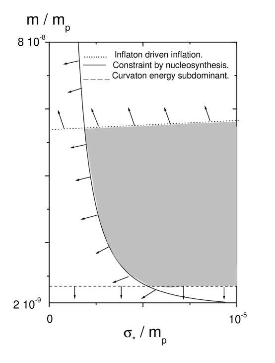
Figure 1: Region of parameter space of model for $m$ versus $\sigma_{*}$. The regions excluded by each constraint are indicated by the arrows, and the allowed region is shaded. We have taken the values : $w=3000$, $(\dot{\Phi}/{\Phi})_{m}=10^{-10}m_{p}$, $\Phi_{m}/\Phi_{eq}=1.25$, $\Phi_{eq}=1.1m_{p}^{2}$, $V_{0}=10^{-11}m_{p}^{4}$ and $\Gamma_{\sigma}=10^{-18}m_{p}$.

The allowed region of the parameter space is reduced for smaller values of the curvaton mass and larger values of curvaton field. This is in agreement with the fact that inflation could take place at smaller - energy scales (smaller than the grand unification scale).

- (1) Guth A., THE INFLATIONARY UNIVERSE: A POSSIBLE SOLUTION TO THE HORIZON AND FLATNESS PROBLEMS, 1981 Phys. Rev. D 23, 347.
- (2) Albrecht A. and Steinhardt P. J., COSMOLOGY FOR GRAND UNIFIED THEORIES WITH RADIATIVELY INDUCED SYMMETRY BREAKING, 1982 Phys. Rev. Lett. 48, 1220; A complete description of inflationary scenarios can be found in the book by Linde A., PARTICLE PHYSICS AND INFLATIONARY COSMOLOGY (Gordon and Breach, New York, 1990).
- (3) Spergel D. N., FIRST YEAR WILKINSON MICROWAVE ANISOTROPY PROBE (WMAP) OBSERVATIONS: DETERMINATION OF COSMOLOGICAL PARAMETERS, 2003 Astrophys. J. Suppl. 148, 175 [astro-ph/0302209]; Peiris H.V., FIRST YEAR WILKINSON MICROWAVE ANISOTROPY PROBE (WMAP) OBSERVATIONS: IMPLICATIONS FOR INFLATION, 2003 Astrophys. J. Suppl. 148, 213 [astro-ph/0302225].
- (4) Berera A., INTERPOLATING THE STAGE OF EXPONENTIAL EXPANSION IN THE EARLY UNIVERSE: A POSSIBLE ALTERNATIVE WITH NO REHEATING, 1997 Phys. Rev. D 55, 3346 [hep-ph/9612239].
- (5) Lyth D. H. and Riotto A., PARTICLE PHYSICS MODELS OF INFLATION AND THE COSMOLOGICAL DENSITY PERTURBATION, 1999 Phys. Rept. B314, 1 [hep-ph/9807278].
- (6) Kolb E. W. and Turner M. S. , The Early Universe, (Addison-Wesley, Menlo Park, Ca., 1990).
- (7) Golgov A. D. and Linde A., BARYON ASYMMETRY IN INFLATIONARY UNIVERSE, 1982 Phys. Lett. B116, 329.
- (8) Kofman L. and Linde A., PROBLEMS WITH TACHYON INFLATION, 2002 JHEP 0207, 004 [hep-th/0205121].
- (9) Felder G., Kofman L. and Linde A., INFLATION AND PREHEATING IN NO MODELS, 1999 Phys. Rev. D60, 103505 [hep-ph/9903350].
- (10) Feng B. and Li M., CURVATON REHEATING IN NONOSCILLATORY INFLATIONARY MODELS, 2003 Phys. Lett. B 564, 169 [ hep-ph/0212213].
- (11) Dine M. , Randall L. and Thomas S., SUPERSYMMETRY BREAKING IN THE EARLY UNIVERSE, 1995 Phys. Rev. Lett. 75, 398 [hep-ph/9503303].
- (12) Dimopoulos K., THE CURVATON HYPOTHESIS AND THE ETA-PROBLEM OF QUINTESSENTIAL INFLATION, WITH AND WITHOUT BRANES, 2003 Phys. Rev. D 68, 123506 [astro-ph/0212264].
- (13) Lucchin F. and Matarrese S., POWER LAW INFLATION, 1985 Phys. Rev. D 32, 1316; Halliwell J., SCALAR FIELDS IN COSMOLOGY WITH AN EXPONENTIAL POTENTIAL, 1987 Phys. Lett. B 185, 341; Barrow J., COSMIC NO HAIR THEOREMS AND INFLATION, 1987 Phys. Lett. B 187, 12.
- (14) Brans C. and Dicke R., MACH’S PRINCIPLE AND A RELATIVISTIC THEORY OF GRAVITATION, 1961 Phys. Rev. 124 , 925.
- (15) Susperregi M. and Mazumdar A., EXTENDED INFLATION WITH AN EXPONENTIAL POTENTIAL, 1998 Phys. Rev. D 58, 083512 [gr-qc/9804081].
- (16) Ford L. H., GRAVITATIONAL PARTICLE CREATION AND INFLATION, 1987 Phys. Rev. D35, 2955.
- (17) Sami M., Chingangbam P. and Qureshi T., ASPECTS OF TACHYONIC INFLATION WITH EXPONENTIAL POTENTIAL, 2002 Phys. Rev. D66, 043530 [hep-th/0205179].
- (18) Liddle A. R. and Ureña-López L. A., CURVATON REHEATING: AN APPLICATION TO BRANE WORLD INFLATION, 2003 Phys. Rev. D68, 043517 [astro-ph/0302054].
- (19) D. H. Lyth and D. Wands, GENERATING THE CURVATURE PERTURBATION WITHOUT AN INFLATON, 2002 Phys. Lett. B524, 5 [hep-ph/0110002].
- (20) Moroi T. and Takahashi T., EFFECTS OF COSMOLOGICAL MODULI FIELDS ON COSMIC MICROWAVE BACKGROUND , 2001 Phys. Lett. B 522, 215 [hep-ph/0110096]; Enqvist K. and Sloth M., ADIABATIC CMB PERTURBATIONS IN PRE - BIG BANG STRING COSMOLOGY, 2002 Nucl. Phys. B 626, 395 [hep-ph/0109214]; Bartolo N. and Liddle A., THE SIMPLEST CURVATON MODEL, 2002 Phys. Rev. D 65, 121301 [astro-ph/0203076].
- (21) Moroi T. and Murayama H., CMB ANISOTROPY FROM BARYOGENESIS BY A SCALAR FIELD, 2003 Phys. Lett. B 553, 126 [hep-ph/0211019]; Enqvist K., Kasuya S. and Mazumdar A., ADIABATIC DENSITY PERTURBATIONS AND MATTER GENERATION FROM THE MSSM, 2003 Phys. Rev. Lett. 90, 091302 [ hep-ph/0211147]; Giovannini M., LOW-SCALE QUINTESSENTIAL INFLATION, 2003 Phys. Rev. D 67, 123512.
- (22) Mollerach S., ISOCURVATURE BARYON PERTURBATIONS AND INFLATION, 1990 Phys. Rev. D 42, 313.
- (23) Campuzano C., del Campo S. and Herrera R., CURVATON REHEATING IN TACHYONIC INFLATIONARY MODELS, 2006 Phys. Lett. B 633, 149 [gr-qc/0511128].
- (24) Campuzano C., del Campo S. and Herrera R., CURVATON REHEATING IN TACHYONIC BRANEWORLD INFLATION, 2005 Phys. Rev. D 72, 083515.
- (25) Joyce M. and Prokopec T., TURNING AROUND THE SPHALERON BOUND: ELECTROWEAK BARYOGENESIS IN AN ALTERNATIVE POSTINFLATIONARY COSMOLOGY, 1998 Phys. Rev. D57, 6022 [hep-ph/9709320].
- (26) Reasenberg R.D., Shapiro I.I., MacNeil P.E., Goldstein R.B., Breidenthal J.C., Brenkle J.P., Cain D.L., Kaufman T.M., Komarek T.A., Zygielbaum A.I., VIKING RELATIVITY EXPERIMENT: VERIFICATION OF SIGNAL RETARDATION BY SOLAR GRAVITY, 1979 Astrophys.J. 234, L219.
- (27) Will C.M., THE CONFRONTATION BETWEEN GENERAL RELATIVITY AND EXPERIMENT. 2001 Living Rev.Rel. 4, 4.
- (28) Guo Z., Piao Y., Cai R. and Zhang Y., INFLATIONARY ATTRACTOR FROM TACHYONIC MATTER, 2003 Phys. Rev. D 68, 043508 [ hep-ph/0304236].
- (29) Lorenz-Petzold D., EXACT PERFECT FLUID SOLUTION IN THE BRANS-DICKE-THEORY, 1984 Astrophysics and Space Science 98, 249.
- (30) Dimopoulos K., Lazarides G., Lyth D. H. and Ruiz de Austri R., CURVATON DYNAMICS, 2003 Phys. Rev. D 68, 123515 [ hep-ph/0308015].
- (31) Postma M., THE CURVATON SCENARIO IN SUPERSYMMETRIC THEORIES, 2003 Phys. Rev. D 67, 063518 [hep-ph/0212005].
- (32) D. H. Lyth, C. Ungarelli and D. Wands, THE PRIMORDIAL DENSITY PERTURBATION IN THE CURVATON SCENARIO, 2003 Phys. Rev. D 67, 023503 [astro-ph/0208055].
- (33) Starobinsky A. and Yokoyama J., in Proccedings of the Fourth Workshop on General Relativity and Gravitation, Kyoto, Japan, 1994, edited by Nakao K. et al. (Kyoto University, Kyoto, 1994); (unpublished) [gr-qc/9502002].
- (34) Starobinsky A., Tsujikawa S. and Yokoyama J., COSMOLOGICAL PERTURBATIONS FROM MULTIFIELD INFLATION IN GENERALIZED EINSTEIN THEORIES 2001 Nucl.Phys.B 610, 383 [astro-ph/0107555].
- (35) Dimopoulos K. and Lyth D. H., MODELS OF INFLATION LIBERATED BY THE CURVATON HYPOTHESIS, 2004 Phys. Rev. D 69, 123509 [hep-ph/0209180].
- (36) Sahni V., Sami M. and Souradeep T., RELIC GRAVITY WAVES FROM BRANE WORLD INFLATION, 2002 Phys. Rev. D65, 023518 [ gr-qc/0105121]; Giovannini M., SPIKES IN THE RELIC GRAVITON BACKGROUND FROM QUINTESSENTIAL INFLATION, 1999 Class. Quant. Grav. 16, 2905 [hep-ph/9903263].
- (37) Ellis J. R., Hagelin J. S., Nanopoulos D. V., Olive K. A. and Srednicki M., SUPERSYMMETRIC RELICS FROM THE BIG BANG, 1984 Nucl. Phys. B 238, 453; Kawasaki M. and Moroi T., GRAVITINO PRODUCTION IN THE INFLATIONARY UNIVERSE AND THE EFFECTS ON BIG BANG NUCLEOSYNTHESIS, 1995 Prog. Theor. Phys. 93, 879 [hep-ph/9403364].
- (38) Gerasimov A. A. and Shatashvili S. L., ON EXACT TACHYON POTENTIAL IN OPEN STRING FIELD THEORY, 2000 JHEP 0010, 034 [ hep-th/0009103]; Kutasov D., Marino M. and Moore G. W., SOME EXACT RESULTS ON TACHYON CONDENSATION IN STRING FIELD THEORY, 2000 JHEP 10, 045 [hep-th/0009148].