CONSTRAINTS ON THE MASS OF A HABITABLE PLANET WITH WATER OF NEBULAR ORIGIN

Abstract

From an astrobiological point of view, special attention has been paid to the probability of habitable planets in extrasolar systems. The purpose of this study is to constrain a possible range of the mass of a terrestrial planet that can get water. We focus on the process of water production through oxidation of the atmospheric hydrogen—the nebular gas having been attracted gravitationally—by oxide available at the planetary surface. For the water production to work well on a planet, a sufficient amount of hydrogen and enough high temperature to melt the planetary surface are needed. We have simulated the structure of the atmosphere that connects with the protoplanetary nebula for wide ranges of heat flux, opacity, and density of the nebular gas. We have found both requirements are fulfilled for an Earth-mass planet for wide ranges of the parameters. We have also found the surface temperature of planets of $\leq 0.3M_{\rm E}$ ($M_{\rm E}$: Earth’s mass) is lower than the melting temperature of silicate ($\sim 1500$  K). On the other hand, a planet of more than several $M_{\rm E}$ becomes a gas giant planet through runaway accretion of the nebular gas.

1 INTRODUCTION

More than 170 extrasolar planets have been detected so far; most of them are Jupiter-like planets (see www.obspm.fr/planets). At present, several projects are in progress to discover terrestrial planets (e.g., TPF, Darwin, etc.). Special attention has thus been paid to habitable planets in extrasolar systems. A prerequisite for a planet being habitable is considered to be the existence of liquid water on it. For a planet to retain liquid water on its surface, it must acquire a sufficient amount of water and be located at a suitable distance from its parent star. This paper focuses on the former issue and constrains the probability of the existence of habitable planets in extrasolar systems.

The latter issue has been discussed using the term “habitable zone”. The habitable zone (HZ) is defined as a range of orbital distance from a star within which a planet can retain liquid water on its surface. Around a solar-mass main-sequence star, the HZ is located around 1 AU and its width is as narrow as $\sim$0.4 AU (Kasting, Whitmire, & Reynolds, 1993). The surface temperature of a planet beyond the HZ is below the freezing temperature of $\rm H_{2}O$, so that the planet is unable to keep liquid water continuously. Because of high surface temperature of a planet closer to its parent star than the HZ, the concentration of $\rm H_{2}O$ in the upper atmosphere is so high that the planet suffers substantial escape of $\rm H_{2}O$ due to incident stellar UV radiation, and ends up losing its ocean completely.

Formation of terrestrial planets in that narrow zone, however, seems to be by no means unlikely within the context of the core accretion model for planet formation. Ida & Lin (2004a, b, 2005), for example, constructed an integrated model for planet formation including the accretion and dynamical evolution of planets. Their model reproduced the mass-period distribution of detected extrasolar planets and also predicted that of unknown planets. In the predicted mass-period distribution, the HZ is filled with hypothetical terrestrial planets of various masses (e.g., Figure 12 of Ida & Lin, 2004a). This means the existence of planets in the HZ is likely; the remaining issue is thus how likely a planet acquires a sufficient amount of water.

In this paper, we consider the nebular origin of water of terrestrial planets. A planet embedded in a protoplanetary nebula attracts gravitationally the nebular gas to have a hydrogen-rich atmosphere (Hayashi, Nakazawa, & Mizuno, 1979; Mizuno, Nakazawa, & Hayashi, 1978). The atmospheric hydrogen can be oxidized by some oxide contained in the planet to produce water on the planet, which was first proposed by Sasaki (1990).

The reason why we focus on the process of water production is that it could commonly happen on any extrasolar terrestrial planet. Planets are in general formed in hydrogen-rich protoplanetary nebulae. Oxides are also available on a terrestrial planet if the C/O ratio of the system is less than unity (Larimer, 1975; Larimer & Bartholomay, 1979); most main-sequence stars are known to have C/O ratios less than unity (e.g., Reddy et al., 2003; Takeda & Honda, 2005). The remaining requirements are a sufficient amount of hydrogen and enough high temperature to melt the surface of the planet; the molten planetary surface being called the magma ocean. The second condition is needed because if the planetary surface remains solid, the reaction between the atmospheric hydrogen and the surface oxide would result just in production of membrane covering the surface, not leading to production of a large amount of water.

In this paper, we investigate properties of the atmosphere of nebular origin. We first clarify the conditions for a planet to have a massive hydrogen-rich atmosphere and a magma ocean to constrain the range of the mass of a planet that has a sufficient amount of water. The structure of the nebular-origin atmosphere was investigated by Hayashi et al. (1979) and Nakazawa et al. (1985) for wide ranges of planetary accretion rate, grain opacity, and density of the nebular gas. However, they used quite simple forms of opacity and equation of state, both of which have been substantially improved. Furthermore they focused only on the Earth (i.e., Earth-mass planets) and had no discussion on the production of water. Although Sasaki (1990) discussed the production of water in order to suggest the deep magma ocean on the early Earth, the ranges of the parameters considered were so restricted that we are unable to get any systematic understanding of the nebular origin of water on terrestrial planets.

We also constrain the mass of a planet that remains a terrestrial one. Habitable planets may be not gas giant but terrestrial ones. If a planet is isolated from planetesimals, it captures a substantial amount of the nebular gas to become a gas giant planet (Ikoma, Nakazawa, & Emori, 2000). We simulate the evolution and accumulation of the planetary atmosphere to obtain the timescale for the substantial gas accretion as a function of planet’s mass. The timescale is compared to the lifetime of the nebular gas of $10^{6}$–$10^{7}$ years (Natta, Grinin, & Mannings, 2000) to constrain a possible range of the mass of a habitable planet.

Section 2 describes our numerical method. Section 3 presents properties of the atmosphere of nebular origin for various planetary masses. Section 4 shows the timescale for the substantial accretion of the nebular gas. Finally we discuss the probability of water production on terrestrial planets and constrain the masses of the potentially-habitable planets in section 5.

2 NUMERICAL METHOD

2.1 Basic equations

We consider a spherically-symmetric hydrostatic atmosphere that connects with the surrounding nebula. The atmospheric structure is determined by the equation of hydrostatic equilibrium including the self-gravity of the atmosphere,

$$\frac{\partial P}{\partial r}=-\frac{GM_{r}\rho}{r^{2}},$$ (1)

and the equation of mass conservation,

$$\frac{\partial M_{r}}{\partial r}=4\pi r^{2}\rho,$$ (2)

where $P$ and $\rho$ are respectively pressure and density of atmospheric gas, $r$ is distance from the planet’s center, $M_{r}$ is mass inside a sphere of radius $r$, and $G$ is the gravitational constant.

The thermal structure is determined by energy transport. If the optical thickness that is defined by

$$\tau\equiv\int_{r}^{R}\kappa\rho dr$$ (3)

is smaller than $2/3$, temperature is given by (Hayashi et al., 1979)

$$T^{4}=T^{4}_{\rm n}+\frac{L}{8\pi\sigma_{\rm SB}r^{2}}\frac{1+3\tau/2}{2-3\tau/2};$$ (4)

in equations (3) and (4), $\tau$ is the optical thickness, $\kappa$ is the Rosseland mean opacity, $R$ is the outer radius of the atmosphere defined below, $T$ and $T_{\rm n}$ are respectively atmospheric and nebular gas temperatures, and $\sigma_{\rm SB}$ is the Stefan-Boltzmann constant. Equation (4) is similar to the well-known formula for radiative transfer in a plane-parallel gray atmosphere, but includes roughly the effect of spherical geometry. Despite of its roughness, we use this convenient formula because quantities of our interest (e.g., surface temperature) are insensitive to the structure of the optically-thin layer.

If $\tau>2/3$, temperature distribution is determined by the smaller of adiabatic and radiative temperature gradients (Kippenhahn & Weiger, 1994): The former is given by

$$\frac{\partial T}{\partial r}=-\frac{GM_{r}\rho}{r^{2}}\left(\frac{\partial T}{\partial P}\right)_{S};$$ (5)

the latter is given by

$$\frac{\partial T}{\partial r}=-\frac{3\kappa\rho L}{64\pi\sigma_{\rm SB}r^{2}T^{3}},$$ (6)

where $S$ is specific entropy and $L$ is energy flux passing through a sphere of radius $r$ (called luminosity). We assume the opacity is the sum of the Rosseland mean opacities of gas molecules and dust grains (see below). The luminosity is determined by (Kippenhahn & Weiger, 1994)

$$\frac{\partial L}{\partial r}=-4\pi r^{2}\rho T\frac{dS}{dt},$$ (7)

where we have assumed there is no energy generation other than entropy change in the atmosphere.

Two types of simulation are done in this paper, quasi-static and static simulations. To calculate the timescale of the gas accretion in section 4, we perform quasi-static simulations integrating all the above equations but equation (4). Inclusion of equation (4) makes the simulation so complicated, but yields little change in the results obtained in section 4. To investigate the properties of the atmosphere extensively in section 3, we perform static simulations integrating equations (1)-(6), because the quasi-static simulations are time-consuming. In the static simulations we assume $L$ is spatially constant, instead of solving equation (7); this assumption was shown to be appropriate for less massive atmospheres (Ikoma et al., 2000).

2.2 Input physics

The equation of state used here is the nonideal one given by Saumon, Chabrier, & Van Horn (1995), interpolated to a composition of $X=0.74$, $Y=0.24$, and $Z=0.02$, where $X$, $Y$, and $Z$ are the mass fractions of hydrogen, helium, and elements heavier than helium, respectively.

The grain opacity is taken from Pollack, McKay, & Christofferson (1985), who presumed dust grains with an interstellar size distribution. Since the amount and size distribution of dust grains in the atmosphere are highly uncertain, we regard the grain opacity as a parameter using the conventional form of $\kappa_{\rm gr}=f\kappa_{\rm gr}^{\rm P}$, where $\kappa_{\rm gr}$ is the grain opacity, $\kappa_{\rm gr}^{\rm P}$ is that given by Pollack et al. (1985), and $f$ is the grain depletion factor.

The gas opacity is taken mainly from Alexander & Ferguson (1994), supplemented with the data of Mizuno (1980); compared to the latter, the opacity for $\rm H_{2}O$ has been substantially improved in the former. In Alexander & Ferguson (1994), data are available for limited ranges of temperature and density, $2.8\leq\log T\leq 4.1$ and $-2\leq\log Q\leq 3$, where $Q=\rho/T_{6}^{3}$, $\rho$ is density in $\rm g\,cm^{-3}$, and $T_{6}$ is temperature in millions of degrees. In the calculations here, we need data for lower temperature and higher density. For $\log T\geq 3.5$ both data sets are similar to each other, because a major source of the opacity is hydrogen for the temperature range. We thus use Mizuno (1980)’s opacity for $\log Q>3$ and $\log T\geq 3.5$. For $2.8\leq\log T\leq 3.5$, a major source of the opacity is $\rm H_{2}O$, and the opacity is rather insensitive to the density. We thus extrapolate values of Alexander & Ferguson (1994) to $\log Q>3$ for that temperature range. For $\log T\leq 2.8$, we adopt values at $\log T=2.8$, because the opacity is nearly constant for $2.8\leq\log T\leq 3.5$.

As mentioned in Introduction, previous workers used rather simple forms of opacity and equation of state. Hydrogen molecules dissociate to hydrogen atoms for the ranges of temperature and density considered here. Hayashi et al. (1979), however, used the equation of state for a perfect gas, although the effect of the dissociation was included in the calculation of the adiabatic temperature gradient. The form of the grain opacity adopted by Hayashi et al. (1979) and Ikoma et al. (2000) was quite simple; the value of the grain opacity was constant until dust grains evaporate at 1500 K independent of gas density. However, the Rosseland mean values of the wavelength-dependent opacity of dust grains depend on temperature and, in reality, dust grains consist of several different components whose evaporation temperatures depend on gas density. Furthermore, as mentioned above, the gas opacity of $\rm H_{2}O$ has been improved and is rather high compared to that used by those workers. For low temperature $\log T<3.5$, $\rm H_{2}O$ makes a dominant contribution to the gas opacity.

2.3 Boundary conditions

Four boundary conditions are needed. Two of the four are given at the bottom of the atmosphere as

$$\begin{array}[]{ccccc}\displaystyle{M_{r}=\frac{4\pi r^{3}}{3}\rho_{\rm s}}&\mbox{and}&L=L_{\rm s}&\mbox{at}&\displaystyle{r=R_{\rm s}\equiv\left(\frac{3M_{\rm s}}{4\pi\rho_{\rm s}}\right)^{1/3},}\end{array}$$ (8)

where $\rho_{\rm s}$, $M_{\rm s}$, and $R_{\rm s}$ are the mean density (= 3.9 $\rm g\,cm^{-3}$), mass, and radius of the solid part of the planet (called simply the solid planet hereafter), respectively, and $L_{\rm s}$ is the energy flux at the surface of the solid planet.

The other two boundary conditions are given at the outer edge of the atmosphere. The outer radius is assumed to be the smaller of the Bondi and the Hill radii, which are respectively defined by

$$R_{\rm B}=\left(1-\frac{1}{\gamma}\right)\frac{GM_{\rm p}}{c_{\rm T}^{2}}$$ (9)

and

$$R_{\rm H}=\left(\frac{M_{\rm p}}{3M_{\ast}}\right)^{1/3}a,$$ (10)

where $M_{\rm p}$ is planetary total mass, $\gamma$ and $c_{\rm T}$ are respectively adiabatic exponent and isothermal sound speed of the nebular gas, $a$ is heliocentric distance, and $M_{\ast}$ is mass of the parent star. At the Bondi radius the enthalpy of gas is equal to the potential energy of gas, while at the Hill radius planetary gravity is equal to the tidal force due to the parent star. For an Earth-mass planet, $R_{\rm B}$ and $R_{\rm H}$ are approximately $20R_{\rm s}$ and $200R_{\rm s}$.

At the outer boundary the atmosphere is assumed to connect smoothly with the nebular gas, namely,

$$\begin{array}[]{ccccc}T=T_{\rm n}&\mbox{and}&P=P_{\rm n}&\mbox{at}&r=R,\end{array}$$ (11)

where $T_{\rm n}$ and $P_{\rm n}$ are the temperature and pressure of the nebular gas. In this paper, $M_{\ast}$ is the solar mass, $a=1\rm AU$, and $T_{\rm n}=280\rm K$, which is the temperature at 1 AU in the minimum-mass solar nebula (Hayashi, 1981). The nebular pressure (equivalently the nebular density) is regarded as a parameter.

2.4 Parameters

The parameters in our atmospheric model for a given planet’s mass ($M_{\rm s}$) are luminosity ($L_{\rm s}$), grain depletion factor ($f$), and the nebular density ($\rho_{\rm n}$).

Because luminosity is supplied by incoming planetesimals in accretion stages, $L_{\rm s}$ is approximately expressed by

$$L_{\rm s}\simeq\frac{GM_{\rm s}}{R_{\rm s}}\dot{M}_{\rm s}=1.1\times 10^{24}\left(\frac{M_{\rm s}}{1M_{\rm E}}\right)^{2/3}\left(\frac{\dot{M}_{\rm s}}{10^{-8}M_{\rm E}\,{\rm yr}^{-1}}\right)\left(\frac{\rho_{\rm s}}{3.9{\rm g\,cm^{-3}}}\right)^{1/3}\rm erg\,s^{-1},$$ (12)

where $\dot{M}_{\rm s}$ is planetesimal accretion rate. The planetesimal accretion rate in late stages of planet formation is uncertain. However, in this paper, since we consider the situations where formation of terrestrial planets is completed before the nebular gas disappears ($10^{6}$–$10^{7}$ years), $M_{\rm s}/\dot{M}_{\rm s}$ should be longer than $\sim 1\times 10^{8}$ years at the time when the planet has grown in mass close to its current mass; otherwise, the planet appreciably grows after the disappearance of the nebula. If $M_{\rm s}/\dot{M}_{\rm s}>1\times 10^{8}$ years, $L_{\rm s}<1\times 10^{24}\rm erg\,s^{-1}$ for an Earth-mass planet and $L_{\rm s}<1\times 10^{23}\rm erg\,s^{-1}$ for a Mars-mass ($\sim$ 0.1 $M_{\rm E}$) planet. A lower limit of luminosity might be constrained by radiogenic luminosity. On the early Earth and Mars, the values of radiogenic luminosity are $\sim 1\times 10^{21}\rm erg\,s^{-1}$ (O’Neill & Palme, 1998) and $\sim 1\times 10^{20}\rm erg\,s^{-1}$ (Wänke & Dreibus, 1988).

The appropriate range of $f$ is also uncertain. Although Podolak (2003) suggested $f\sim 0.01$ through the numerical simulations of coagulation and sedimentation of dust grains in the atmosphere, more extensive study is needed because their simulations were performed only in a few atmospheric models. We thus consider $f=0$–$1$ in this paper.

The nebular gas dissipates with time. Taking it into account, we consider a wide range of the nebular density, 1–$10^{-10}$ times the gas density ($\rho_{\rm MSN}=1.2\times 10^{-9}\rm g\,cm^{-3}$ at 1 AU) of minimum-mass solar nebula model (Hayashi, 1981) for the Earth-mass case.

3 PROPERTIES OF THE ATMOSPHERE

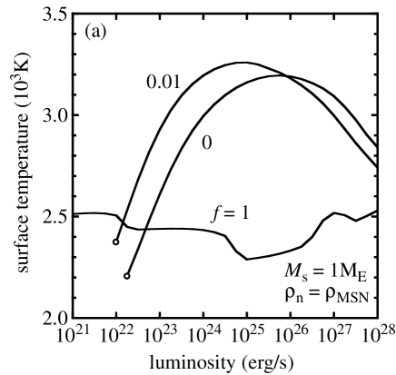
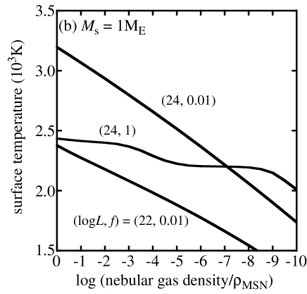
Figure 1: The surface temperature (i.e., the temperature at the bottom of the atmosphere) of an Earth-mass planet for wide ranges of three parameters, luminosity ($L$), grain depletion factor ($f$), and density of the nebular gas ($\rho_{\rm n}$). In (a), the surface temperature is shown as a function of $L$ for three different values of $f$. In (b), the surface temperature is shown as a function of $\rho_{\rm n}$ normalized by that in the minimum-mass solar nebula ($\rho_{\rm MSN}=1.2\times 10^{-9}\rm g\,cm^{-3}$) for three different sets of values of $L$ and $f$. The attached sets of values are $\log L$ in $\rm erg\,s^{-1}$ and $f$ in (b). Circles represent critical luminosities (see the text).

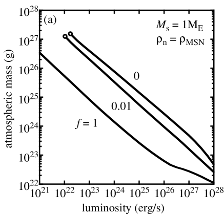
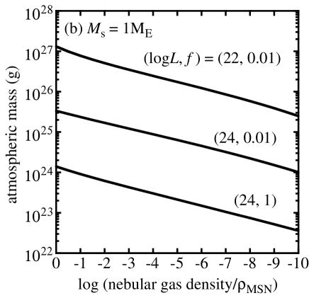
Figure 3: The atmospheric mass of an Earth-mass planet for wide ranges of three parameters, luminosity ($L$), grain depletion factor ($f$), and density of the nebular gas ($\rho_{\rm n}$). In (a), the atmospheric mass is shown as a function of $L$ for three different values of $f$. In (b), the atmospheric mass is shown as a function of $\rho_{\rm n}$ normalized by that in the minimum-mass solar nebula ($\rho_{\rm MSN}=1.2\times 10^{-9}\rm g\,cm^{-3}$) for three different sets of values of $L$ and $f$. The attached sets of values are $\log L$ in $\rm erg\,s^{-1}$ and $f$. Circles represent critical luminosities (see the text).

Figure 1a illustrates that the surface temperature of an Earth-mass planet changes only by at most 50 % despite of the order-of-magnitude differences in luminosity and grain opacity, and is always higher than 2000 K when $\rho_{\rm n}=\rho_{\rm MSN}$. The shapes of the functions for $f=0$ and $0.01$ are convex. The atmosphere is largely radiative for lower luminosities, whereas it is largely convective for higher luminosities. Although surface temperature in general increases with luminosity for radiative atmospheres, its dependence is found to be weak. This is because the effect of higher luminosity is almost compensated for with that of smaller optical depth (i.e., smaller mass of the atmosphere) that is due to high luminosity as shown below (see Fig. 3a). For fully convective atmospheres, any atmospheric property is independent of luminosity. As luminosity increases, the inner convective region expands outward, but, at the same time, the optically-thin, almost isothermal layer also extends inward because of a decrease in atmospheric mass. The latter effect is responsible for the decrease in surface temperature for high luminosities. The complicated form of the function for $f=1$ comes from the complicated form of the grain opacity; several different components evaporate at different temperatures depending on gas density.

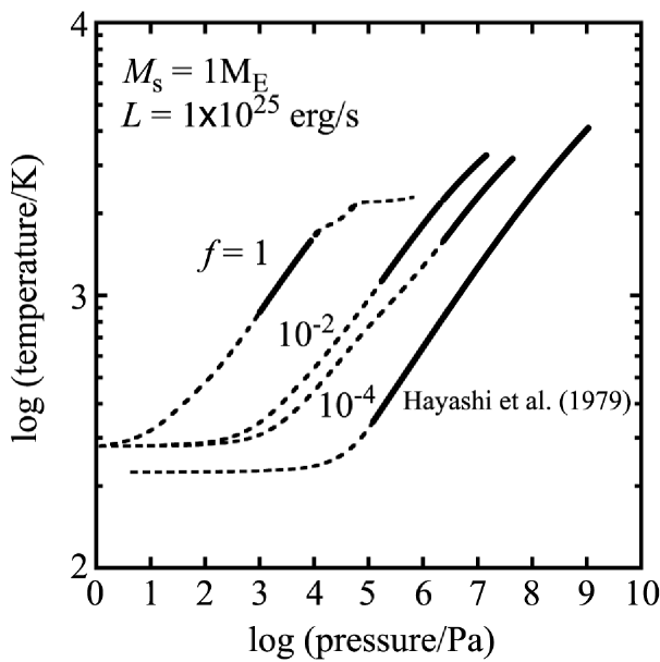
Figure 2: The atmospheric structure of an Earth-mass planet for three different values of grain depletion factor ($f$) and luminosity ($L$) of $1\times 10^{25}\rm erg\,s^{-1}$. The structure simulated in the similar way to Hayashi et al. (1979) is also shown; in the simulation we have adopted $\rho_{\rm n}=5.7\times 10^{-9}\rm g\,cm^{-3}$ and $T_{\rm n}=225\rm K$, following Hayashi et al. (1979). The bold and dashed lines represent convective and radiative layers, respecitively.

The surface temperature for $f=1$ is clearly lower than that for $f\leq 0.01$. To understand the difference, we compare the atmospheric structure for $f=1$, 0.01, and $1\times 10^{-4}$ in Fig. 2. This figure illustrates that the low surface temperature for $f=1$ comes mainly from sudden decreases in temperature gradient due to evaporation of silicate around 2000 K. For $f\leq 0.01$, pressure increases substantially in the optically-thin layer and is so high at the evaporation temperature that convection takes place at that point; the evaporation of silicate thus has no influence on the structure.

The values of surface temperature obtained here ($<$  3300 K) are lower than $\sim$ 4000 K obtained by Hayashi et al. (1979). Their analytical calculation for a polytropic atmosphere also yielded $\sim$ 4000 K. In Fig. 2 we show the atmospheric structure calculated in the similar way to Hayashi et al. (1979), using Mizuno (1980)’s gas opacity and the grain opacity of $1\times 10^{-4}\rm cm^{2}\,g^{-1}$ for $T\leq$ 1500 K. The grain opacity of $1\times 10^{-4}\rm cm^{2}\,g^{-1}$ is lower than gas opacity even in the low-temperature region. As described in section 2, our gas opacity is much higher than that used by Hayashi et al. (1979). Because of the lower opacity in Hayashi et al. (1979)’s model, the isothermal layer is deeper, resulting in a large increase in pressure. As a result, in Hayashi et al. (1979)’s calculation, the atmosphere is almost fully convective except for the isothermal layer. As shown in Appendix, surface temperature for a convective atmosphere is slightly higher than that for a radiative atmosphere (e.g., eq. [A17]). This may be the reason why the surface temperature for $f=1\times 10^{-2}$ and $1\times 10^{-4}$ is slightly lower than that obtained by Hayashi et al. (1979).

As shown in Fig. 1b, the surface temperature of an Earth-mass planet is rather insensitive to the nebular density. A decrease in the nebular density certainly lowers surface temperature because of a decrease in optical depth, but it changes only by a factor of less than two even if the nebular density decreases by ten orders of magnitude. Figure 1b shows the surface temperature of an Earth-mass planet is always higher than 1500 K, the typical melting temperature of silicate, for a wide range of the nebular density. The insensitivity of the surface temperature of an Earth-mass planet to luminosity, opacity, and the nebular density is analytically explained in Appendix. As also shown in Appendix, it is a rather robust conclusion that the surface temperature of an Earth-mass planet is higher than the melting temperature of silicate.

As shown in Fig. 3a, atmospheric mass decreases almost linearly with luminosity and grain depletion factor (for $f>0.01$). Lower luminosity and opacity yield gentler temperature gradient (see eq. [6]). Then, density gradient must be steeper to maintain sufficiently large pressure gradient that supports the gravity. Since the density is fixed at the outer edge, the steep density profile results in a massive atmosphere. It should be noted that in Fig. 3a a curve ends off at a critical low value of luminosity at which the atmospheric mass is comparable with the planetary mass. Beyond the point no static solution is found. That means substantial gas accretion takes place if luminosity is smaller than the critical value (see section 4).

Atmospheric mass decreases as the nebular density decreases, which is shown in Fig. 3b. However the dependence is found to be rather weak. Most of the atmospheric mass is concentrated in the deep atmosphere. And, as shown in Appendix, the structure of the deep atmosphere is insensitive to the outer boundary conditions.

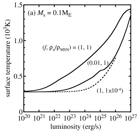
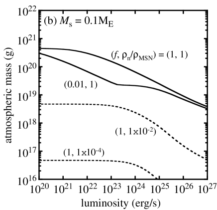
Figure 4: The surface temperature (a) and atmospheric mass (b) of a 0.1 $M_{\rm E}$ planet are shown as functions of luminosity for several different sets of values of grain depletion factor ($f$) and density of the nebular gas ($\rho_{\rm n}$) normalized by that in the minimum-mass solar nebula ($\rho_{\rm MSN}=1.2\times 10^{-9}\rm g\,cm^{-3}$).

The atmosphere on a Mars-mass ($\sim 0.1M_{\rm E}$) planet exhibits different behaviour compared to that on an Earth-mass planet shown above. Figure 4 shows surface temperature (a) and atmospheric mass (b) as functions of luminosity for several choices of grain depletion factor ($f$) and the nebular density ($\rho_{\rm n}$). Unlike the case of an Earth-mass planet, the surface temperature of an Mars-mass planet is sensitive to luminosity and grain opacity. The dependence of the atmospheric mass of an Mars-mass planet on those parameters is different from that of an Earth-mass planet. In Fig. 4a surface temperature is shown to appreciably decrease as luminosity decreases. Although atmospheric mass increases with decreasing luminosity in the similar way to the Earth-mass case for high luminosities, there is upper limits to atmospheric mass. Comparing Figs. 4a and 4b, we find that when the atmospheric mass reaches the upper limit, surface temperature reaches the nebular temperature ($=280$ K), which means the atmosphere is almost isothermal as a whole. As shown in Fig. 4, the surface temperature and atmospheric mass of a Mars-mass planet are also sensitive to the nebular density, which is also different from the Earth-mass case. The atmospheric mass decreases almost linearly with decreasing nebular density. A mathematical explanation for the difference between Earth-mass and Mars-mass cases is given in Appendix.

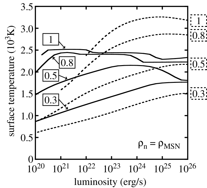
Figure 5: Surface temperature as a function of luminosity for several choices of planet’s mass. Each attached number represents planet’s mass in the Earth mass. The solid and dashed lines represent cases of $f=1$ and $0.01$, respectively.

Figure 5 shows surface temperature as a function of luminosity for four choices of planet’s mass (0.3, 0.5, 0.8, and 1 $M_{\rm E}$), two values of $f$ (0.01 and 1), and $\rho_{\rm n}=\rho_{\rm MSN}$. Smaller planetary mass yields lower surface temperature for given $L_{\rm s}$ and $f$ (e.g., see eq. [A17]). The surface temperature for $M_{\rm s}=0.8M_{\rm E}$ exhibits the “Earth-type” behaviour that surface temperature is not so sensitive to a decrease in luminosity, while that for $M_{\rm s}=0.3M_{\rm E}$ exhibits the “Mars-type“ behaviour that surface temperature is sensitive to a decrease in luminosity. The case of a $0.5M_{\rm E}$ planet seems to be marginal. As regards melting of the surface of the solid planet that occurs when surface temperature is higher than typically 1500 K, the melting is very unlikely on a $0.3M_{\rm E}$ planet even if the planet is embedded in the nebula of density as high as that of the minimum-mass solar nebula, as shown in Fig. 5.

4 TIMESCALE FOR GAS ACCRETION

As mentioned in section 3, no static solution is found below a critical value of the luminosity. That means energy supply due to atmospheric contraction is needed to keep the atmosphere in hydrostatic equilibrium. The contraction results in substantial accretion of the nebular gas to make the planet a gas-giant one. In reality, this happens once the planet becomes isolated from planetesimals. In order to exclude gas giant planets from the group of habitable planets, we investigate the timescale for the gas accretion (i.e., the timescale for a planet to grow up to be a gas giant planet). The gas accretion is known to occur not always in a runaway fashion: Its typical timescale increases considerably, as the mass of the solid planet decreases (Ikoma et al., 2000).

The timescale for the gas accretion also depends on the opacity. As described in section 2, Ikoma et al. (2000) used a rather simple form of the grain opacity adopted by Mizuno (1980), while we use more complicated and realistic grain opacity given by Pollack et al. (1985). The values of Pollack et al. (1985)’s grain opacity are larger by a factor of approximately 10 than those of Mizuno (1980)’s for a temperature range from $\sim 200$ K to $\sim 1000$ K. Also, unlike Mizuno (1980)’s grain opacity, Pollack et al. (1985)’s depends on gas density because the evaporation temperature of rock becomes high with gas density.

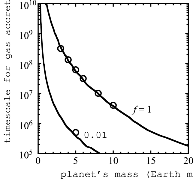
Figure 6: The typical timescale for substantial accretion of the nebular gas as a function of planet’s mass for two choices of the grain depletion factor ($f$). The open circles represent the numerical results of our evolutionary calculations; the solid lines are drawn using equation (13) with the numerical factor $\alpha$ of 1/3.

Figure 6 shows the typical timescale for the gas accretion ($t_{\rm g}$) after planetesimal accretion is suddenly terminated; on this timescale a planet becomes a Jupiter-like planet. Following Ikoma et al. (2000), we define $t_{\rm g}$ as follows. We first calculate the purely-hydrostatic structure of the atmosphere for given values of $M_{\rm s}$ and $L_{\rm s}$ (see eq. [8]). Then, setting $L_{\rm s}$ to be zero, we start quasi-static simulation of the evolution and accumulation of the atmosphere. The luminosity emitted from the outer edge of the atmosphere soon decreases to a minimum value and, then, increases progressively (see Fig. 2b of Ikoma et al., 2000). Most of the gas-accretion phase is spent when the luminosity is near the minimum value. The minimum luminosity is almost equal to the above-mentioned critical luminosity (Ikoma et al., 2000). The characteristic time for growth of atmospheric mass—$M_{\rm a}/\dot{M}_{\rm a}$ where $M_{\rm a}$ is atmospheric mass and $\dot{M}_{\rm a}$ is gas accretion rate—at the minimum luminosity obtained by the quasi-static calculations are plotted with open circles in Fig. 6. Although we are unable to obtain the timescale for the gas accretion for $f<0.01$ because the simulations for $f<0.01$ is quite time-consuming, the result is expected to be similar to that for $f=0.01$, because difference in $f$ ($<0.01$) yields only small difference in atmospheric mass (see Fig. 3a).

The timescale $t_{\rm g}$ is approximated by (Ikoma et al., 2000)

$$t_{\rm g}=\alpha\frac{GM_{\rm s}M_{\rm a}^{\ast}}{R_{\rm conv}^{\ast}L^{\ast}},$$ (13)

where $L^{\ast}$ is the critical luminosity, $M_{\rm a}^{\ast}$ and $R_{\rm conv}^{\ast}$ are the atmospheric mass and outer radius of the inner convective layer at $L=L^{\ast}$. The curves in Fig. 6 are drawn using equation (13) with the value of each quantity obtained by our static calculation and $\alpha=1/3$. Those curves are fitted roughly by

$$t_{\rm g}=1\times 10^{10}f\left(\frac{M_{\rm s}}{M_{\rm E}}\right)^{-3.5}{\rm yr}$$ (14)

for $f\geq 0.01$. Not only the value of $t_{\rm g}$ itself but also its dependence on the mass of the solid planet obtained here are different from those by Ikoma et al. (2000) in which $t_{\rm g}\sim 1\times 10^{8}f(M_{\rm s}/M_{\rm E})^{-2.5}$ yr. In particular $t_{\rm g}$ for $M_{\rm s}=1M_{\rm E}$ is 100 times as large as that given by Ikoma et al. (2000). This is because our grain opacity is larger than theirs. And this is also because our grain opacity depends on gas density unlike theirs. For smaller planetary mass, the critical luminosity is small. Then the density for a given temperature is high relative to high-luminosity cases, so that the evaporation temperatures are also high. Thus the effective grain opacity is higher for smaller planetary masses.

Similar calculations for a few values of planet’s mass were also done by Hubickyj, Bodenheimer, & Lissauer (2005). The equation of state and the gas and grain opacity tables they used were almost the same as those we have used here. We compare our results with their results of the duration ($t_{\rm g}^{\rm HBL}$) between the end of Phase 1 (at which planetesimal accretion was suddenly terminated) and the crossover point (at which envelope mass is equal to core mass) in the models named 10H5 and 10H10 in which core masses are approximately $5M_{\rm E}$ and $10M_{\rm E}$, respectively, and $f=1$. Although we are unable to exactly compare our results to theirs because the definition of $t_{\rm g}^{\rm HBL}$ is not exactly equal to that of $t_{\rm g}$, both values are found to be similar: For $M_{\rm s}=5M_{\rm E}$, $t_{\rm g}\simeq 62\rm Myr$ while $t_{\rm g}^{\rm HBL}\simeq 78\rm Myr$; for $M_{\rm s}=10M_{\rm E}$, $t_{\rm g}\simeq 4\rm Myr$ while $t_{\rm g}^{\rm HBL}\simeq 3\rm Myr$.

5 DISCUSSION

Based on the numerical results obtained in sections 3 and 4, we discuss production of water from the hydrogen-rich atmosphere on a terrestrial planet, a possible range of the mass of a habitable planet, and the possibility of the nebular origin of water on the Earth.

As described in Introduction, production of water on a terrestrial planet requires a sufficient amount of hydrogen and surface temperature higher than the melting temperature of silicate ($\sim$ 1500 K). The two conditions are found to be fulfilled on an Earth-mass planet.

In a late stage of terrestrial planet formation, accretion rate of planetesimals (i.e., luminosity) decreases with time because of exhaustion of the planet’s feeding zone. The decrease in luminosity increases the amount of hydrogen on an Earth-mass planet (see Fig. 3a), while surface temperature remains above 2000 K (see Fig. 1a). For example, if accretion rate of planetesimals is $1\times 10^{-9}M_{\rm E}\,{\rm yr^{-1}}$, corresponding to $L\sim 1\times 10^{23}\rm erg\,s^{-1}$ (see eq. [12]), the mass of atmospheric hydrogen is more than about $1\times 10^{25}$ g for $f<1$, as shown Fig. 3a: The amount of hydrogen a planet acquires is insensitive to the nebular density (see Fig. 3b).

Water is produced through reaction between the atmospheric hydrogen and oxides contained in the solid planet. The amount of water depends on what kind of oxide is available. Ion oxides (e.g., wüstite [$\rm Fe_{0.974}O$], magnetite [$\rm Fe_{3}O_{4}$], etc.) and fayalite ($\rm Fe_{2}SiO_{4}$) react with the atmospheric hydrogen to produce water comparable in mass to hydrogen; the ratios of the partial pressures, $P_{\rm H_{2}O}/P_{\rm H_{2}}$, are 0.88, 24.02, and 0.49 at 1500 K for the iron-wüstite ($\rm 1.894Fe+O_{2}\leftrightarrow 2Fe_{0.947}O$), the wüstite-magnetite ($\rm 6.696Fe_{0.974}O+O_{2}\leftrightarrow 2.174Fe_{3}O_{4}$), and the quartz-iron-fayalite oxygen ($\rm 2Fe+SiO_{2}+O_{2}\leftrightarrow Fe_{2}SiO_{4}$) buffers, respectively (Robie, Hemingway, & Fisher, 1978). Thus, if a planet acquires hydrogen of $\sim 1\times 10^{25}\rm g$ and such oxygen buffers are available, the planet obtains water comparable in mass to the current sea water on the Earth ($=1.4\times 10^{24}$ g). However, for the silicon-periclase-forsterite buffer ($\rm 2MgO+Si+O_{2}\leftrightarrow Mg_{2}SiO_{4}$), $P_{\rm H_{2}O}/P_{\rm H_{2}}$ is as small as $\sim 3\times 10^{-7}$ (Robie et al., 1978). Fe-bearing minerals might be required to produce sufficient water, although how much water is needed for a planet being habitable is quite uncertain. Whether Fe-bearing minerals commonly exist in extrasolar systems is still a matter of controversy. Equilibrium condensation in a highly-reduced environment like a protoplanetary nebula yields not Fe-bearing minerals but Fe-metal (Wood & Hashimoto, 1993). However, dust grains in a protoplanetary nebula can be considered to have non-equilibrium composition including, at least, fayalite (Pollack et al., 1994, and references therein).

When the surrounding nebular gas disappears almost completely, the atmosphere and solid planet begin to get cold, and then an ocean forms through the condensation of steam in the atmosphere. However, almost complete dissipation of the nebular gas allows the extremely ultraviolet (EUV) and far-UV radiation from the parent star to penetrate the planetary atmosphere. Such irradiation causes extensive loss of hydrogen (and steam). The timescale for complete loss of a $10^{25}$-g (say) hydrogen-rich atmosphere due to EUV and far-UV can be estimated to be longer than $10^{6}$ years (Sekiya, Nakazawa, & Hayashi, 1980, 1981), if very strong EUV and far-UV (up to 100 times higher than the present; Guinan & Ribas, 2002) from the young parent star is considered. On the other hand, the timescale for the ocean formation is on the order of $10^{3}$ years on a planet located in the HZ, according to calculations based on the radiative-convective equilibrium model of an $\rm H_{2}O$-$\rm CO_{2}$ atmosphere with mass of $\sim 10^{24}$ g (Abe, 1993). The timescale for the ocean formation for a $\rm H_{2}O$-$\rm H_{2}$ atmosphere considered here is probably not so different from that for an $\rm H_{2}O$-$\rm CO_{2}$ atmosphere, because inclusion of $\rm H_{2}$ hardly affects the atmospheric structure due to its weak blanketing effect. Therefore, an ocean can forms before the significant loss of the atmosphere due to EUV and far-UV.

We can constrain a possible range of the mass of a habitable planet. As shown in section 3, there is a lower limit to the planetary mass below which the water production proposed in this paper does not work. Figure 5 illustrates that surface temperature of a planet of $\leq$ 0.3 $M_{\rm E}$ is lower than the melting temperature of silicate ($\sim 1500$ K) for reasonable ranges of the parameters. On the other hand, an upper limit to the mass of a habitable planet can be constrained because a massive planet captures a huge amount of the nebular gas to be a gas giant planet, not a terrestrial planet. The timescale for the gas accretion depends strongly on the planetary mass, as shown Fig. 6. This timescale should be compared to the lifetime of the nebula that is known to be about $1\times 10^{7}$ years (Natta, Grinin, & Mannings, 2000). The comparison suggests that the upper limit to the planetary mass is $7M_{\rm E}$ for $f=1$ and $2M_{\rm E}$ for $f=0.01$.

The water production proposed in this paper may have worked on our Earth. Because of N-body simulations of planetary accretion, details of the terrestrial planet formation in the solar system have been clarified. After the runaway growth of protoplanets (Wetherill & Stewart, 1993), they grow in an oligarchic fashion until they eat almost all of the planetesimals in their feeding zones (Kokubo & Ida, 1998, 2000). Then several Mars-mass protoplanets form in the terrestrial planet region. The subsequent growth of the protoplanets needs giant impacts between them. The planets formed in the way is likely to have high eccentricities (Chambers, Wetherill, & Boss, 1996). Damping of those high eccentricities needs the drag force of the nebular gas (Kominami & Ida, 2002; Nagasawa, Lin, & Thommes, 2005). Because the Earth is isolated in the nebular gas, the accretion of the nebular gas inevitably takes place and water is produced on the Earth. Although the amount of the nebular gas required for the damping of the eccentricities are as small as $10^{-4}$ to $10^{-3}$ times that of the minimum-mass solar nebula (Kominami & Ida, 2002; Nagasawa et al., 2005), our numerical results show that this small amount of the nebular gas is sufficient for the Earth to get water comparable in mass with Earth’s sea water.

We should be, however, careful when we consider the nebular origin of water on the Earth. This is because the ratio of deuterium to hydrogen (D/H) of the sea water on the present Earth is larger by about a factor of seven than D/H of the solar nebula (e.g., Drake & Righter, 2002). Moreover, the current Earth’s atmosphere includes a tiny amount of noble gas, while the solar nebula was rich in noble gas (e.g., Pepin, 1991). The latter problem may be solved by extensive loss of the noble gases as well as hydrogen from the atmosphere due to EUV and far-UV radiation (Sekiya et al., 1980, 1981). Although adequate mixing of water originated from nebular gas and water in comets can produce the present D/H on the Earth’s ocean, because D/H in comets is larger (by about a factor of two) than D/H of the present Earth’s ocean (e.g., Drake & Righter, 2002), the former problem is difficult to solve. At present, we have no definite evidences that the sea water of the Earth was originated from the nebular gas.

Our intention in this paper is to claim that water production from the nebular gas on a planet is a possible way for a terrestrial planet in the HZ to acquire water. As shown in this paper, the water production works, if a planet of 0.3 to several $M_{\rm E}$ forms in the protoplanetary nebula. The probability of formation of terrestrial planets in the nebular gas is still open to debate, mainly because the dissipation mechanism of the nebular gas is quite uncertain. However, the existence of many gas giant planets in extrasolar planets has ensured the validity of the core accretion model. That is, accretion of planets generally occurs in a protoplanetary nebula. Also, there is no good reason for terrestrial planet formation to prefer vacuum environment. Therefore, it is rather likely that terrestrial planets also form in the surrounding nebular gas. The production of water from the nebular gas in the HZ thus seems to be a natural consequence of planet formation.

Appendix A Analytical solutions of the atmospheric structure

Analytical consideration of the atmospheric structure gives a deep insight into the atmospheric properties shown in section 3. Here we focus on surface temperature and check whether surface temperature exceeds the melting temperature of silicate ($\sim$ 1500 K). In the following analytical consideration, we make some additional assumptions: (1) The atmospheric self-gravity is negligible; (2) the atmospheric gas is perfect gas with constant mean molecular weight and adiabatic exponent; (3) opacity and luminosity are constant. The first assumption is reasonable because the atmospheric mass is negligibly small relative to the mass of a solid planet in cases of our interest. Although the second assumption breaks down for $T>2000$–3000 K because of dissociation of $\rm H_{2}$, we adopt it because the temperature range of interest is $<$ 1500 K. The third assumption is just for simplicity, but the opacity does not change so much (within less than one order of magnitude) for $T<1500\rm K$.

We adopt the following dimensionless variables,

$$\begin{array}[]{lllcl}\displaystyle{\varpi=\frac{P}{P_{0}}},&\displaystyle{\sigma=\frac{\rho}{\rho_{0}}},&\displaystyle{\theta=\frac{T}{T_{0}}},&\mbox{and}&\displaystyle{x=\frac{r}{R_{0}}},\end{array}$$ (A1)

where quantities with suffices 0 are reference quantities. On the above assumptions, using those variables, the hydrostatic equation is written by

$$\frac{1}{\sigma}\frac{d\varpi}{dx}=-\frac{V_{0}}{x^{2}},$$ (A2)

and equation of state is written by

$$\varpi=\sigma\theta.$$ (A3)

The equations for convective and radiative energy transports are respectively given by

$$\varpi = \sigma^{\gamma},$$ (A4)

$$\frac{d\theta^{4}}{d\varpi} = W_{0},$$ (A5)

In the above set of equations,

$$V_{0}=\frac{GM_{\rm s}\rho_{0}}{R_{0}P_{0}}=\frac{GM_{\rm s}\mu m_{\rm H}}{kR_{0}T_{0}},$$ (A6)

where $\mu$ is the mean molecular weight, $m_{\rm H}$ is the mass of a hydrogen atom, and $k$ is the Boltzmann constant;

$$W_{0} = \frac{3\kappa LP_{0}}{16\pi\sigma_{\rm SB}GM_{\rm s}T_{0}^{4}}$$ (A7)

$$= 4.3\times 10^{-3}\left(\frac{M_{\rm s}}{1M_{\rm E}}\right)^{-1}\left(\frac{\kappa}{1\rm cm^{2}\,g^{-1}}\right)\left(\frac{L}{10^{24}\rm erg\,s^{-1}}\right)\left(\frac{P_{0}}{1\rm Pa}\right)\left(\frac{T_{0}}{280\rm K}\right)^{-4}.$$ (A8)

For later discussion, we define an additional quantity $\lambda$ as

$$\lambda = \frac{GM_{\rm s}\rho_{0}}{R_{\rm s}P_{0}}$$ (A9)

$$= \frac{\gamma}{\gamma-1}\frac{R_{\rm B}}{R_{\rm s}}=56\left(\frac{M_{\rm s}}{1M_{\rm E}}\right)^{2/3}\left(\frac{T_{0}}{280\rm K}\right)^{-1}\left(\frac{\mu}{2.34}\right)\left(\frac{\rho_{\rm s}}{3.9\rm g\,cm^{-3}}\right)^{1/3},$$ (A10)

where we have used 7/5 for $\gamma$.

We can obtain the exact solutions for the set of equations (A2)–(A5). The convective solution is given by

$$\theta=1+\frac{\gamma-1}{\gamma}V_{0}\left(\frac{1}{x}-1\right),$$ (A11)

while the radiative solution is given by

$$\frac{1}{x}=1+\frac{1}{V_{0}}\left\{4\left(\theta-1\right)+F\left(\theta,W_{0}\right)\right\},$$ (A12)

where

$$F(\theta,W_{0})=w_{0}\left[\ln\left(\frac{\theta-w_{0}}{\theta+w_{0}}\frac{1+w_{0}}{1-w_{0}}\right)-2\left(\arctan\frac{\theta}{w_{0}}-\arctan\frac{1}{w_{0}}\right)\right]$$ (A13)

for $W_{0}<1$;

$$w_{0}\equiv\left(1-W_{0}\right)^{1/4}.$$ (A14)

The exact solution for $W_{0}>1$ can be also obtained (Inaba & Ikoma, 2003).

The dimensionless surface temperature ($\theta_{\rm s}$) for a fully convective atmosphere is given by

$$\theta_{\rm s}=\frac{1}{x_{\rm s}}=\frac{\gamma-1}{\gamma}\lambda,$$ (A15)

since $R_{0}=R_{\rm B}$ and thus $V_{0}=\gamma/(\gamma-1)$; $\theta_{\rm s}$ for a fully radiative atmosphere is given by

$$\theta_{\rm s}=\frac{V_{0}}{4}\frac{1}{x_{\rm s}}=\frac{\gamma}{4(\gamma-1)}\frac{1}{x_{\rm s}}=\frac{\lambda}{4},$$ (A16)

if $\theta_{\rm s}\gg 1$ and $x_{\rm s}\ll 1$. The dimensionless surface temperature is found to be determined only by $\lambda$. Thus, surface temperature is given by

$$T_{\rm s}=\left\{\begin{array}[]{l}4500\\ 3900\end{array}\right\}\left(\frac{M_{\rm s}}{1M_{\rm E}}\right)^{2/3}\left(\frac{\mu}{2.34}\right)\left(\frac{\rho_{\rm s}}{3.9\rm g\,cm^{-3}}\right)^{1/3}\rm K,$$ (A17)

where the upper and lower values are for the convective ($\gamma=7/5$) and radiative cases, respectively. Those solutions were also given by Hayashi et al. (1979). The surface temperature given by equation (A17) is determined only by planet’s mass (for given $\mu$ and $\rho_{\rm s}$) and independent of luminosity, opacity, and outer boundary conditions.

The above conclusion is consistent with the numerical results for an Earth-mass planet but in contradiction with those for a Mars-mass planet given in section 3. To understand the discrepancy, we compare the exact solution (A12) with the approximate one (A16); the result is shown in Fig. 7. The difference is found to depend on the value of $W_{0}$. For an Earth-mass planet, the difference is only 40 % even for $\log W_{0}=-10$ and the exact value of $T_{\rm s}\sim$ 2300 K, while, for a Mars-mass planet, the difference is more sensitive to $W_{0}$ and the exact $T_{\rm s}$ reaches $T_{0}$ at $\log W_{0}=-4$. From a mathematical point of view, the sensitivity is more remarkable for smaller value of $\lambda$.

The existence of the outermost isothermal layer lowers surface temperature. To check how much surface temperature is reduced, we simulate the structure of a two-layer atmosphere composed of the outer isothermal layer and the inner radiative or convective layer. We first determine the radius of the photosphere where the optical depth defined by equation (3) is equal to 2/3, using the isothermal solution

$$\sigma=\exp\left[V_{0}\left(\frac{1}{x}-1\right)\right].$$ (A18)

Once we obtained values of the quantities at the photosphere, checking convective stability, we calculate surface temperature using equation (A11) or (A12). Figure 8 shows the surface temperature as a function of $\rho_{\rm n}/\rho_{\rm MSN}$ for six different values of $\kappa$ and $L=1\times 10^{21}\rm erg\,s^{-1}$; The solid and dashed lines representing convective and radiative lower layers, respectively. If we adopt higher values of luminosity, we obtain higher temperatures for $\kappa\geq 1\times 10^{-4}\rm cm^{2}\,g^{-1}$. As shown in Fig. 8, even if luminosity is as small as $1\times 10^{21}\rm erg\,s^{-1}$, surface temperature is above the melting temperature of silicate ($\simeq$ 1500 K) except for a limited range of the nebular density, $\rho_{\rm n}<1\times 10^{-6}\rho_{\rm MSN}$.

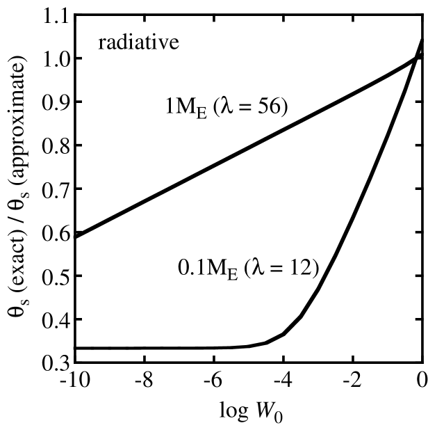
Figure 7: Difference in value of the dimensionless surface temperature ($\theta_{\rm s}$) between the exact radiative solution (eq. [A12]) and the approximate radiative solution called the radiative-zero solution (eq. [A16]) for two cases of 1 $M_{\rm E}$ and 0.1 $M_{\rm E}$ planets. The definitions of $W_{0}$ and $\lambda$ are given by equations (A7) and (A9), respectively.

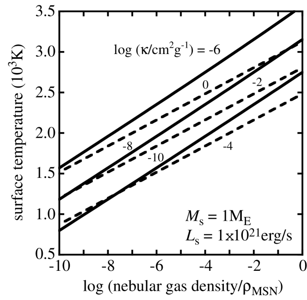
Figure 8: The surface temperature of an Earth-mass planet as a function of density of the nebular gas that is normalized by that of the minimum-mass solar nebula ($\rho_{\rm MSN}=1.2\times 10^{-9}\rm g\,cm^{-3}$) for six different values of opacity ($\kappa$) and luminosity ($L_{\rm s}$) of $1\times 10^{21}\rm erg\,s^{-1}$ that has been analytically obtained in the two-layer (outer isothermal and inner radiative or convective) atmospheric model (see Appendix). The solid and dashed lines respectively convective anr radiative inner atmospheres.

References

- Abe (1993) Abe, Y. 1993, Lithos 30, 223
- Alexander & Ferguson (1994) Alexander, D. R., & Ferguson, J. W. 1994, ApJ437, 879
- Chambers, Wetherill, & Boss (1996) Chambers, J. E., Wetherill, G. W., & Boss A. P. 1996, Icarus119, 261
- Drake & Righter (2002) Drake, M. J., & Righter, K. 2002, Nature416, 39
- Guinan & Ribas (2002) Guinan, E. F., & Ribas, I. 2002, in ASP Conf. Ser. 269, The Evolving Sun and Its Influence on Planetary Environments, ed. B. Montesinos, A. Gimenez, & E. F. Guinan (San Francisco: ASP), 85
- Hayashi (1981) Hayashi, C. 1981. Prog. Theor. Phys. Suppl. 70, 35
- Hayashi et al. (1979) Hayashi, C., Nakazawa, K., & Mizuno, H. 1979, EPSL 43, 22
- Hubickyj et al. (2005) Hubickyj, O., Bodenheimer, P., & Lissauer, J. J. 2005, Icarus179, 415
- Ida & Lin (2004a) Ida, S., & Lin, D. N. C. 2004a, ApJ604, 388
- Ida & Lin (2004b) Ida, S., & Lin, D. N. C. 2004b, ApJ616, 567
- Ida & Lin (2005) Ida, S., & Lin, D. N. C. 2005, ApJ626, 1045
- Ikoma et al. (2000) Ikoma, M., Nakazawa, K., & Emori, H. 2000, ApJ537, 1013
- Inaba & Ikoma (2003) Inaba, S., & Ikoma, M. 2003, A&A410, 711
- Kasting, Whitmire, & Reynolds (1993) Kasting, J. F., Whitmire, D. P., & Reynolds, R. T. 1993, Icarus101, 108
- Kippenhahn & Weiger (1994) Kippenhahn, R., & Weigert, A. 1994, in Stellar Structure and Evolution (Berlin: Springer-Verlag)
- Kokubo & Ida (1998) Kokubo, E., & Ida, S. 1998, Icarus131, 171
- Kokubo & Ida (2000) Kokubo, E., & Ida, S. 2000, Icarus143, 15
- Kominami & Ida (2002) Kominami, J., & Ida, S. 2002, Icarus157, 43
- Larimer (1975) Larimer, J. W. 1975, Geochim. Cosmochim. Acta39, 389
- Larimer & Bartholomay (1979) Larimer, J. W., & Bartholomay M. 1979, Geochim. Cosmochim. Acta43, 1455
- Mizuno (1980) Mizuno, H. 1980, Prog. Theor. Phys., 64, 544
- Mizuno et al. (1978) Mizuno, H., Nakazawa, K., & Hayashi, C. 1978, Prog. Theor. Phys. 60, 699
- Nakazawa et al. (1985) Nakazawa, K., Mizuno, H., Sekiya, M., & Hayashi, C. 1985, J. Geomag. Geoelectr. 37, 781
- Nagasawa et al. (2005) Nagasawa, M., Lin, D. N. C., & Thommes, E. 2005, ApJ, 635, 578
- Natta, Grinin, & Mannings (2000) Natta, A., Grinin, V., & Mannings, V. 2000, in Protostars & Planets IV, ed. V. Mannings, A. Boss & S. Russell (Tucson: Univ. Arizona Press), 559
- O’Neill & Palme (1998) O’Neill, H. C., & Palme, H. 1998, in The Earth’s Mantle, ed. J. Jackson (Chambridge: Chambridge Univ. Press), 3
- Pepin (1991) Pepin, R. O. 1991, Icarus92, 2
- Podolak (2003) Podolak, M. 2003, Icarus165, 428
- Pollack et al. (1985) Pollack, J. B., McKay, C. P., & Christofferson, B. M. 1985, Icarus64, 471
- Pollack et al. (1994) Pollack, J. B., Hollenbach, D., Beckwith, S., Simonelli, D. P., Roush, T., & Fong, W. 1994, ApJ421, 615
- Reddy et al. (2003) Reddy, B. E., Tomkin, J., Lambert, D. L., & Allende Prieto, C. 2003, MNRAS340, 304
- Robie et al. (1978) Robie, R. A., Hemingway, B. S., & Fisher, J. R. 1978, U.S. Geol. Surv. Bill. 1452
- Sasaki (1990) Sasaki, S. 1990, in Origin of the Earth, ed. H. E. Newson & J. H. Jones (New York: Oxford Univ. Press), 195
- Saumon, Chabrier, & Van Horn (1995) Saumon, D., Chabrier, G., & Van Horn, H. M. 1995, ApJS99, 713
- Sekiya et al. (1980) Sekiya, M., Nakazawa, K., & Hayashi, C. 1980, Prog. Theor. Phys. 64, 1968
- Sekiya et al. (1981) Sekiya, M., Hayashi, C., & Nakazawa, K. 1981, Prog. Theor. Phys. 66, 1301
- Takeda & Honda (2005) Takeda, Y., & Honda, S. 2005, PASJ 57, 65
- Wänke & Dreibus (1988) Wänke, H., & Dreibus, G. 1988, Phil. Trans. Roy. Soc. London, A235, 545
- Wetherill & Stewart (1993) Wetherill, G. W., & Stewart, G. R. 1993, Icarus106, 190
- Wood & Hashimoto (1993) Wood, J. A., & Hashimoto, A. 1993, Geochim. Cosmochim. Acta57, 2377
- Zahnle (1993)