Mass-loss properties of S-stars on the AGB

We have used a detailed non-LTE radiative transfer code to model new APEX CO($J$ $=$ 3 $\rightarrow$ 2) data, and existing CO radio line data, on a sample of 40 AGB S-stars. The derived mass-loss-rate distribution has a median value of 2 $\times$ 10^-7 M_⊙ yr^-1, and resembles values obtained for similar samples of M-stars and carbon stars. Possibly, there is a scarcity of high-mass-loss-rate ($\geq$ 10^-5 M_⊙ yr^-1) S-stars. The distribution of envelope gas expansion velocities is similar to that of the M-stars, the median is 7.5 km s^-1, while the carbon stars, in general, have higher gas expansion velocities. The mass-loss rate correlates well with the gas expansion velocity, in accordance with results for M-stars and carbon stars.

1 Introduction

Stars of spectral class S are identified through their strong bands of primarily ZrO. This indicates enhancements of s-process elements. It is now relatively well-established that these enhancements can be produced in two ways: through dredge-up of nuclear-processed material during the asymptotic giant branch (AGB) evolution (intrinsic S-star), or through mass transfer in a binary system (extrinsic S-star). The strong bands of ZrO in intrinsic S-stars, as opposed to the strong bands of TiO in M-stars, have been attributed to a stellar atmosphere chemistry in a relatively low-temperature ($\la$ 3000 K) gas enriched in s-process elements and with C/O $=$ 1 (within about 5%) (Scalo & Ross 1976; Smith & Lambert 1990). This then lead to the belief that the AGB S-stars are transition objects between AGB M-stars and carbon stars.

Extensive mass loss is a key process during the evolution of AGB stars. M-stars and carbon stars lose substantial amounts of matter during this phase, and their mass-loss characteristics are relatively well-established (see Olofsson 2003). The putative transition objects, the S-stars, have attracted less attention in this respect. Studies of CO radio line and dust continuum emission suggest that they behave in roughly the same way as both their predecessors and descendants in terms of mass-loss rate, circumstellar kinematics, dust composition, and dust-to-gas ratio (Jura 1988; Bieging & Latter 1994; Sahai & Liechti 1995; Groenewegen & de Jong 1998; Jorissen & Knapp 1998).

In this Letter new APEX CO($J$ $=$ 3 $\rightarrow$ 2) data, in combination with existing CO radio line data and a radiative transfer code, were used to derive the circumstellar properties of 40 S-stars on the AGB.

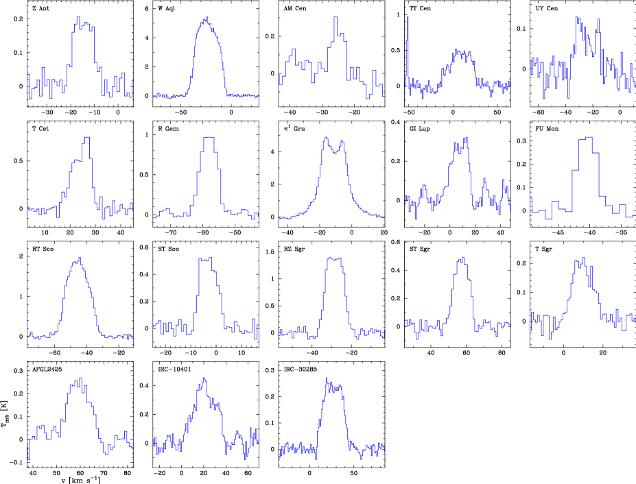
Figure 1: New observations of CO($J$ $=$ 3$\rightarrow$ 2) line emission using the APEX telescope. The velocity resolution is 1.0 km s^-1.

2 Observations

The sample was selected from the list of 65 objects with S-star characteristics in the Two Micron Sky Survey by Wing & Yorka (1977) [see also Jura (1988)]. Observations of CO $J$ $=$ 3 $\rightarrow$ 2 line emission at 345.80 GHz towards a sample of 18 S-stars were performed from August to October 2005 using the APEX 12 m telescope equipped with a double-sideband SIS receiver and a FFTS spectrometer. The system temperature (above atmosphere) varied between 130 and 335 K. The effective bandwidth at the observations were 1 GHz with a spectral resolution of 61 kHz (0.05 km s^-1), except for FU Mon, R Gem, and Z Ant observed during the second run with a spectral resolution of 122 kHz (0.11 km s^-1). The data was smoothed to 1 km s^-1 resolution and reduced by removing a low-order ($\leq$ 3) polynomial baseline in the range of about $\pm$ 100 km/s from the stellar velocity. The resulting spectra are presented in Figure. 1, and velocity-integrated intensities are reported in Table 1.

The observations were carried out using a position-switching mode, with the reference position located +2$\arcmin$ in azimuth. The raw spectra are stored in the $T_{\mathrm{A}}^{\star}$ scale and converted to main-beam brightness temperature using $T_{\mathrm{mb}}$ = $T_{\mathrm{A}}^{\star}/\eta_{\mathrm{mb}}$, where $T_{\mathrm{A}}^{\star}$ is the antenna temperature corrected for atmospheric attenuation using the chopper-wheel method, and $\eta_{\mathrm{mb}}$ the main-beam efficiency, estimated to be 0.7 at 345 GHz. The uncertainty of the absolute intensity scale is estimated to be about $\pm$ 20%. Regular pointing checks were made on strong CO sources and typically found to be consistent within $\approx$ 3$\arcsec$. The FWHM of the main beam, $\theta_{\mathrm{mb}}$, is 18$\arcsec$ at 345 GHz.

In addition to the new APEX data presented here, we have also used new CO($J$ $=$ 1 $\rightarrow$ 0) data observed at the Onsala 20 m telescope ( January 2006), JCMT public archive CO data, and CO line intensities reported by Bieging & Latter (1994), Sahai & Liechti (1995), Stanek et al. (1995), Groenewegen & de Jong (1998), and Jorissen & Knapp (1998). In total, 42 S-stars have been detected in CO line emission.

3 Radiative transfer analysis

In our analysis the circumstellar envelopes (CSEs) are assumed to be spherically symmetric, to be produced by a constant mass-loss rate ($\dot{M}$), and to expand at a constant velocity ($v_{\mathrm{e}}$). The spectra of $\pi^{1}$ Gru and RS Cnc indicate that deviations from the standard CSE model are present and no modelling was attempted for these two sources (see Sahai 1992; Knapp et al. 1999).

3.1 SED modelling

The SEDs were constructed from IRAS-fluxes and 2MASS-magnitudes. The continuum emission was modelled using the dust radiative transfer code DUSTY (Ivezić & Elitzur 1997). Amorphous carbon or amorphous silicate dust was selected based on, in most cases, the spectral class of the IRAS low-resolution spectra as defined by Volk & Cohen (1989). In the cases where the spectral class was not available, the selection was based on colour-colour diagrams as described by Jorissen & Knapp (1998). The adopted dust type is listed in Table 1, where C and O denotes carbon and silicate dust, respectively. The amount of dust present in the wind can be constrained from the spectral shape of the SED. Details on the modelling procedure can be found in Schöier et al. (2002) and Ramstedt et al. (2006).

The SED results were used in combination with the luminosities to estimate the distances to the sample stars. Luminosities of the Miras were estimated using the period-luminosity relation of Whitelock et al. (1994). For the semi-regular and irregular variables, a luminosity of 4000 $\mathrm{L_{\odot}}$ was assumed in accordance with Olofsson et al. (2002). Corrections for interstellar extinction were applied. The derived distances and adopted luminosities are listed in Table 1. Non-negative Hipparcos parallaxes with an accuracy better than 50 % are available for seven of the sample stars. They agree well within the error margins, when compared to the distances derived from the SED modelling (except for RZ Peg).

The results from the SED modelling were also used to determine the dust radiation field which is important for the excitation of CO.

Table 1: APEX observations and model summary

$\begin{array}[]{p{0.162\linewidth}cccccccccc}\hline\cr\vskip 3.0pt plus 1.0pt minus 1.0pt\cr&&&&\lx@intercol\hfil\mathrm{CO\ modelling}\hfil\lx@intercol\\ \vskip 3.0pt plus 1.0pt minus 1.0pt\cr\cline{5-10}\cr\vskip 3.0pt plus 1.0pt minus 1.0pt\cr\lx@intercol\hfil{\mathrm{Source}}\hfil\lx@intercol&\lx@intercol\hfil D\hfil\lx@intercol&\lx@intercol\hfil L_{\star}\hfil\lx@intercol&\lx@intercol\hfil I(\mathrm{3-2})\hfil\lx@intercol&\lx@intercol\hfil\dot{M}\hfil\lx@intercol&\lx@intercol\hfil v_{\mathrm{e}}\hfil\lx@intercol&\lx@intercol\hfil h\hfil\lx@intercol&\lx@intercol\hfil\chi^{2}_{\mathrm{red}}\hfil\lx@intercol&\lx@intercol\hfil N\hfil\lx@intercol&\lx@intercol\hfil{\mathrm{dust}}\hfil\lx@intercol\\ &\lx@intercol\hfil[\mathrm{pc}]\hfil\lx@intercol&\lx@intercol\hfil[\mathrm{L_{\odot}}]\hfil\lx@intercol&\lx@intercol\hfil[\mathrm{Kkms^{-1}}]\hfil\lx@intercol&\lx@intercol\hfil[\mathrm{M_{\odot}\,yr^{-1}}]\hfil\lx@intercol&\lx@intercol\hfil[\mathrm{kms^{-1}}]\hfil\lx@intercol&&&&\lx@intercol\hfil{\mathrm{type}}\hfil\lx@intercol\\ \vskip 3.0pt plus 1.0pt minus 1.0pt\cr\hline\cr\vskip 3.0pt plus 1.0pt minus 1.0pt\cr\object{R And}\,${}^{b}$&300&6000&\cdots&6.0\times 10^{-7}&8.0&0.2$:$&0.1&2&$O$\\ \object{W And}\,${}^{a}$&280&5800&\cdots&1.2\times 10^{-7}&5.5&0.2$:$&1.0&3&$O$\\ \object{Z Ant}&470&4000&2.0&9.0\times 10^{-8}&6.0&0.2$:$&\cdots&1&$O$\\ \object{VX Aql}&790&4000&\cdots&5.0\times 10^{-8}&7.0$:$&0.2$:$&\cdots&1&$C$\\ \object{W Aql\,$^{c}$ }&230&6800&136&2.5\times 10^{-6}&17.5&0.7&2.5&4&$O$\\ \object{AA Cam}&800&4000&\cdots&1.8\times 10^{-7}&16.9$:$&0.2$:$&\cdots&1&$C$\\ \object{T Cam}&540&5600&\cdots&1.0\times 10^{-7}&4.8$:$&0.2$:$&\cdots&1&$C$\\ \object{S Cas}\,${}^{a,b}$&440&8000&\cdots&2.2\times 10^{-6}&19.0&0.5$:$&0.9&2&$O$\\ \object{V365 Cas}&625&4000&\cdots&3.0\times 10^{-8}&6.2$:$&0.2$:$&\cdots&1&$C$\\ \object{WY Cas}&600&6700&\cdots&6.0\times 10^{-7}&12.5$:$&0.5$:$&\cdots&1&$O$\\ \object{AM Cen}&750&4000&1.1&1.5\times 10^{-7}&3.3&0.2$:$&1.9&2&$C$\\ \object{TT Cen}&880&6500&13.9&2.5\times 10^{-6}&20.0&0.5$:$&7.8&2&$O$\\ \object{UY Cen}&590&4000&1.6&1.2\times 10^{-7}&12.0&0.2$:$&\cdots&1&$C$\\ \object{V386 Cep}&470&4000&\cdots&1.8\times 10^{-7}&18.6$:$&0.2$:$&\cdots&1&$O$\\ \object{T Cet}\,${}^{a,b,c,d}$&240&4000&3.7&5.0\times 10^{-8}&5.5&0.2&0.8&4&$C$\\ \object{AA Cyg}&480&4000&\cdots&4.0\times 10^{-7}&6.1$:$&0.2$:$&\cdots&1&$C$\\ \object{R Cyg}\,${}^{a}$&440&6100&\cdots&5.0\times 10^{-7}&9.5&0.5$:$&1.8&3&$O$\\ \object{$\chi$ Cyg}\,${}^{a,b,c}$&110&5900&\cdots&5.0\times 10^{-7}&8.5&0.1&2.0&3&$O$\\ \object{TV Dra}\,${}^{a}$&390&4000&\cdots&7.0\times 10^{-8}&4.0&0.2$:$&\cdots&1&$O$\\ \object{DY Gem}&680&4000&\cdots&1.3\times 10^{-7}&7.0&0.2$:$&\cdots&1&$O$\\ \object{R Gem}\,${}^{a}$&710&5500&6.4&4.0\times 10^{-7}&4.0&0.5$:$&1.0&2&$C$\\ \object{ST Her}\,${}^{a}$&300&4000&\cdots&1.3\times 10^{-7}&8.5&0.2$:$&1.1&3&$O$\\ \object{RX Lac}&310&4000&\cdots&6.5\times 10^{-8}&5.5$:$&0.2$:$&\cdots&1&$C$\\ \object{GI Lup}&690&5000&4.6&1.0\times 10^{-6}&10.0&0.2$:$&\cdots&1&$C$\\ \object{R Lyn}\,${}^{a}$&850&5600&\cdots&3.0\times 10^{-7}&7.0&0.2$:$&0.2&2&$C$\\ \object{Y Lyn}\,${}^{a}$&260&4000&\cdots&1.7\times 10^{-7}&7.0&0.2$:$&\cdots&1&$O$\\ \object{S Lyr}&1210&6300&\cdots&1.0\times 10^{-6}&13.0$:$&0.5$:$&\cdots&1&$O$\\ \object{FU Mon}&780&4000&1.3&1.2\times 10^{-7}&2.0&0.2$:$&\cdots&1&$C$\\ \object{RZ Peg}&970&4000&\cdots&3.4\times 10^{-7}&12.6$:$&0.2$:$&\cdots&1&$C$\\ \object{RT Sco}&270&6400&32.6&4.5\times 10^{-7}&11.0&0.5$:$&3.2&2&$O$\\ \object{ST Sco}&380&4000&4.5&1.3\times 10^{-7}&5.5&0.2$:$&1.2&3&$O$\\ \object{RZ Sgr}&730&4000&15.8&1.5\times 10^{-5}&9.0&0.2$:$&22.3&2&$C$\\ \object{ST Sgr}&540&5800&4.9&2.7\times 10^{-7}&7.0&0.2$:$&3.0&2&$O$\\ \object{T Sgr}&590&5800&2.5&2.0\times 10^{-7}&10.0&0.2$:$&\cdots&1&$C$\\ \object{EP Vul}&510&4000&\cdots&1.5\times 10^{-7}&4.4$:$&0.2$:$&5.5&2&$C$\\ \object{DK Vul}&750&4000&\cdots&6.0\times 10^{-7}&4.0$:$&0.2$:$&\cdots&1&$C$\\ \object{AFGL2425}&610&4000&2.8&2.0\times 10^{-7}&6.5&0.2$:$&0.9&2&$O$\\ \object{CSS2 41}&880&4000&\cdots&6.0\times 10^{-7}&20.0$:$&0.2$:$&\cdots&1&$O$\\ \object{IRC-30285}&590&4000&6.5&6.0\times 10^{-7}&17.0&0.2$:$&6.0&2&$O$\\ \object{IRC-10401}&430&4000&9.5&3.5\times 10^{-7}&17.0&0.2$:$&12.8&2&$O$\\ \vskip 3.0pt plus 1.0pt minus 1.0pt\cr\hline\cr\end{array}$

Superscripts mark new or archive data: ^a OSO $J$ = 1 $\rightarrow$ 0,
^b JCMT $J$ = 3 $\rightarrow$ 2 , ^c JCMT $J$ = 4 $\rightarrow$ 3, ^d JCMT $J$ = 6 $\rightarrow$ 5.
The forth column gives the APEX $J$ = 3 $\rightarrow$ 2 results.

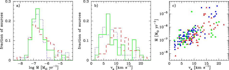
Figure 2: a) Mass-loss-rate distributions for the S-star (solid line; 40 stars), M-star (dotted line; 77 stars), and carbon star (dashed line; 61 stars) samples. b) Envelope gas expansion velocity distributions for the S-star (solid line), M-star (dotted line), and carbon star (dashed line) samples. c) Derived mass-loss rates plotted against the gas expansion velocities for the S-star (dots), M-star (squares), and carbon star (triangles) samples.

3.2 Radiative transfer model

In order to determine the molecular excitation in the CSE, a detailed non-LTE radiative transfer code, based on the Monte Carlo method, was used. This code is described in detail in Schöier & Olofsson (2001). It has been benchmarked, to high accuracy, against a wide variety of molecular-line radiative transfer codes in van Zadelhoff et al. (2002).

The CO molecules are partly excited through collisions with H₂. The collisional rate coefficients calculated by Flower (2001) were adopted and extended to include more energy levels as well as extrapolated in temperature (see Schöier et al. 2005). An ortho-to-para ratio of 3 was adopted when weighting together collisional rate coefficients for CO in collisions with ortho- and para-H₂. The excitation analysis includes radiative excitation through the first vibrationally excited ($v$ = 1) state at 4.6 $\mu$m. Relevant molecular data are summarised in Schöier et al. (2005) and are made publicly available through the Leiden Atomic and Molecular Database (LAMDA). A central blackbody was assumed to represent the stellar radiation field, and thermal, circumstellar dust emission was included. These provide the main sources of the infrared photons that excite the $v$ = 1 state. The addition of a dust component in the Monte Carlo scheme is straightforward as described in Schöier et al. (2002). The energy-balance equation was solved simultaneously as the excitation of CO, allowing for an accurate determination of the kinetic gas temperature of the gas. The photospheric abundance of CO, relative to H₂, was assumed to be 6 $\times$ 10^-4. A micro-turbulent velocity of 1 km s^-1 was assumed.

Two parameters are adjustable when fitting the model to the observed line intensities: the mass-loss rate ${\dot{M}}$ and the $h$-parameter. The latter is a product of different dust parameters (Schöier et al. 2002). Collisional heating through gas colliding with dust grains is the dominant heating term in the energy-balance equation and it affects the model line-intensity ratios. We were able to constrain $h$ for five of our stars. Its dependence on stellar luminosity is consistent with our findings for M-stars (Olofsson et al. 2002) and carbon stars (Schöier & Olofsson 2001). Therefore, a value was assumed for the remaining stars depending on the stellar luminosity, $h$=0.2 for $L$ $<$ 5000 L_⊙ and $h$=0.5 above 5000 L_⊙ (indicated by a colon in Table 1).

The best-fit model was found by minimizing the difference between the observed and modelled integrated line intensities ($N$, in Table 1, is the number of observed lines used). Reduced $\chi^{2}$-values were calculated and are presented in Table 1, when a sufficient number of lines were available. The uncertainties in the derived mass-loss rates were estimated to be about $\pm$ 50% within the adopted circumstellar model, excluding distance uncertainties, in accordance with Schöier & Olofsson (2001) and Olofsson et al. (2002).

A particular problem occurred with the CO($J$ = 2 $\rightarrow$ 1) data. We found a large scatter in the reported intensities for an individual object, even when observed with the same telescope. Furthermore, these data are, in general, not compatible with the model results, i.e., the 3 $\rightarrow$ 2/1 $\rightarrow$ 0 intensity ratios are compatible with the model results, while the 2 $\rightarrow$ 1/1 $\rightarrow$ 0 or 3 $\rightarrow$ 2/2 $\rightarrow$ 1 intensity ratios are, in general, not (note, the model line-intensity ratios only weakly depend on the assumed parameters). Consequently, we decided to omit the 2 $\rightarrow$ 1 data from our analysis, except for the few cases where only a 2 $\rightarrow$ 1 line exists.

4 Results and discussion

We compare here our results for the S-star sample, which were obtained through detailed radiative transfer modelling, with those obtained in the same way for a sample of M-stars (Olofsson et al. 2002) and a sample of carbon stars (Schöier & Olofsson 2001). The samples are flux-limited but not complete, except for the carbon-star sample, which contains a subsample that is most likely complete out to a distance of 500 pc (Schöier & Olofsson 2001). The incompleteness of the samples and the small number statistics limit the generality of our conclusions.

Figure 2a shows the mass-loss-rate distribution of the S-star sample in comparison with those of the M-stars and the carbon stars. The S-star mass-loss-rate distribution appears very similar to that of the M-stars and the carbon stars. The median value is 2 $\times$ 10^-7 M_⊙ yr^-1 for the M- and S-star samples, and 3 $\times$ 10^-7 M_⊙ yr^-1 for the carbon-star sample. There is possibly fewer S-stars with a high mass-loss rate ($\geq$ 10^-5 M_⊙ yr^-1). Figure 2b shows the expansion velocity distribution of the S-star sample in comparison with those of the M-stars and carbon star samples. There is an indication that the carbon stars have higher expansion velocities, while those of the S- and M-stars appear similar. The median expansion velocity is 7.5 km s^-1 for the S-star and M-star samples, and 11 km s^-1 for the carbon star sample. Figure 2c shows that the relations between mass-loss rate and envelope expansion velocity are very similar for the three samples, pointing towards the same mass-loss mechanism.

This is the first step in a project aimed at obtaining an extensive data base of circumstellar molecular lines towards a sample of S-stars. The CO data will constrain the circumstellar model, and accurate molecular abundances will be derived. These will be compared with results of chemical modelling, as well as with the results for the M-star and carbon star samples.