TeV lightcurve of PSR B1259-63/SS2883

Abstract

The inverse Compton (IC) scattering of ultrarelativistic electrons accelerated at the pulsar wind termination shock is generally believed to be responsible for TeV gamma-ray signal recently reported from the binary system PSR B1259-63/SS2883. While this process can explain the energy spectrum of the observed TeV emission, the gamma-ray fluxes detected by HESS at different epochs do not agree with the published theoretical predictions of the TeV lightcurve. The main objective of this paper is to show that the HESS results can be explained, under certain reasonable assumptions concerning the cooling of relativistic electrons, by inverse Compton scenarios of gamma-ray production in PSR B1259-63. In this paper we study evolution of the energy spectra of relativistic electrons under different assumptions about the acceleration and energy-loss rates of electrons, and the impact of these processes on the lightcurve of IC gamma-rays. We demonstrate that the observed TeV lightcurve can be explained (i) by adiabatic losses which dominate over the entire trajectory of the pulsar with a significant increase towards the periastron, or (ii) by the ”early” (sub-TeV) cutoffs in the energy spectra of electrons due to the enhanced rate of Compton losses close to the periastron. The first four data points obtained just after periastron comprise an exception - possibly due to interaction with the Be star disk, which introduces additional physics not included in the presented model. The calculated spectral and temporal characteristics of the TeV radiation provide conclusive tests to distinguish between these two working hypotheses. The Compton deceleration of the electron-positron pulsar wind contributes to the decrease of the nonthermal power released in the accelerated electrons after the wind termination, and thus to the reduction of the IC and synchrotron components of radiation close to the periastron. Although this effect alone cannot explain the observed TeV and X-ray lightcurves, the Comptonization of the cold ultrarelativistic wind leads to the formation of gamma-radiation with a specific line-type energy spectrum. While the HESS data already constrain the Lorentz factor of the wind, $\Gamma\leq 10^{6}$ (for the most likely orbit inclination angle $i=35^{\circ}$, and assuming an isotropic pulsar wind), future observations of this object with GLAST should allow a deep probe of the wind Lorentz factor in the range between $10^{4}$ and $10^{6}$.

1 Introduction

PSR B1259-63/SS 2883 – a binary system consisting of a 47ms pulsar orbiting around a luminous Be star (Johnston et al., 1992) – is a unique high energy laboratory for the study of nonthermal processes related to the ultrarelativistic pulsar winds. X-ray and gamma-ray emission components are expected from this object due to the radiative (synchrotron and inverse Compton) cooling of relativistic electrons accelerated by the wind termination shock (Tavani & Arons, 1997; Kirk et al., 1999). Generally, the particle acceleration in this complex system can be treated as a scaled-down in space and time (”compact and fast”) realization of the current paradigm of Pulsar Wind Nebulae (PWN) which suggests that the interaction of the ultrarelativistic pulsar wind with surrounding medium leads to the formation of a relativistic standing shock (Rees & Gunn, 1974; Kennel & Coroniti, 1984; Harding & Gaisser, 1990; Tavani & Arons, 1997). In the case of strong and young pulsars, the shock-accelerated multi-TeV electrons should give rise to observable X-ray (synchrotron) and TeV (inverse Compton) nebulae with typical linear size $\sim 0.1-10$ pc. The unambiguous association of some of the recently discovered extended TeV gamma-ray sources with several distinct synchrotron X-ray PWNs generally supports this scenario of formation of nonthermal nebulae around the pulsars.

In the binary system PSR B1259-63/SS 2883 one should expect a similar mechanism of conversion of the major fraction of the rotational energy of the pulsar to ultrarelativistic electrons through formation and termination of the cold electron-positron wind. On the other hand, in such systems the magnetohydrodynamic (MHD), acceleration and radiation processes proceed under essentially different conditions compared to the PWN around isolated pulsars. In particular, due to the high pressure of the ambient medium caused by the outflow from the companion star, the pulsar wind terminates quite close to the pulsar, $R\leq 10^{12}$ cm. Consequently, in such systems particle acceleration occurs at presence of much stronger magnetic field ($B\sim 0.1-1$ G), and under illumination of intense radiation from the normal star with a density

$$w_{\rm ph}={L_{\rm star}\over 4\pi cR^{2}}\sim 0.9\left(L_{\rm star}\over 3.3\cdot 10^{37}{\rm erg/s}\right)\left(R\over 10^{13}{\rm cm}\right)^{-2}\ {\rm erg/cm^{3}}\,,$$ (1)

where $L_{\rm star}$ is the luminosity of the Be star and $R$ is the distance between the acceleration site and the Be star. The discussed ranges of the temperature and the luminosity of the star SS2883 vary within $T\simeq 2.3\cdot 10^{4}-2.7\cdot 10^{4}{\rm K}$ and $L_{\rm star}\simeq 3.3\cdot 10^{37}-2.2\cdot 10^{38}{\rm erg/s}$. This implies that both the acceleration and radiative cooling timescales of TeV electrons are of order of hours, i.e. comparable or shorter than the typical dynamical timescales characterizing the system. This allows a unique ”on-line watch” of the extremely complex MHD processes of creation and termination of the ultrarelativistic pulsar wind and the subsequent particle acceleration, through the study of spectral and temporal characteristics of high energy gamma-radiation of the system. The discovery of TeV gamma-radiation from PSR B1259-63/SS2883 by HESS collaboration (Aharonian et al., 2005) provides the first unambiguous evidence of particle acceleration in such systems to TeV energies.

Remarkably, in spite of the complexity of the binary system PSR B1259-63/SS2883, one may calculate with quite high precision the spectral and temporal features of gamma-radiation based on only a few model assumptions concerning, in particular, the magnetic field, the acceleration rate as well as the non-radiative (adiabatic or escape) losses of electrons. The observational uncertainties involved in these calculations are mainly related to the luminosity of the optical companion SS 2883. The basic free parameters used in calculations are the rates of particle acceleration and the nonradiative losses caused by adiabatic expansion and escape of electrons.

The orbital elements of the system are well known. The orbit is quite eccentric ($e=0.87$) with the minimum and maximum distances between the pulsar and the star $D_{\rm 0}=9.6\times 10^{12}{\rm cm}$ and $D_{\rm a}=1.4\times 10^{14}{\rm cm}$ at the periastron and the apastron, respectively; the inclination of orbit is $i\simeq 35^{\circ}$ (Johnston et al., 1992). The separation between the pulsar and the optical companion versus the epoch is shown in Fig.1. In the same figure we show the possible locations of pulsar passage through the stellar disk as discussed by Johnston et al. (2005) and Chernyakova et al. (2006). In the first paper the disk location is determined by the time of disappearance of the pulsed radio emission which is explained by absorption of the pulsar emission in the stellar disk. However, as long as the physics of interaction of the pulsar winds with the stellar disk is not firmly established, alternative models are not excluded. For example, Chernyakova et al. (2006) noticed that the maxima of lightcurves of nonpulsed radio, X-ray and TeV gamma-ray are quite close to each other, and proposed that the increase of the nonthermal energy release happens when the pulsar crosses the disk. If so, the gamma-ray emission could be result of hadronic interactions (Kawachi et al., 2004; Chernyakova et al., 2006). This hypothesis implies, however, a different location of the disk compared to the one derived from the eclipse of the pulsed radio emission (Johnston et al., 2005; Bogomazov, 2005), and therefore requires an independent confirmation based on a stronger evidence of correlation of radio, X-ray and TeV fluxes, as well as detailed study of the reasons of such correlation.

Meanwhile, the inverse Compton scattering remains the most plausible gamma-ray production mechanism (Tavani & Arons, 1997; Kirk et al., 1999; Aharonian et al., 2005). In this paper we present detailed numerical studies of the the spectral and temporal characteristics of TeV gamma-ray emission within the framework of the IC model of TeV gamma-rays. In this context we adopt the position of the disk as it is derived from the eclipse of pulsed radio emission (Johnston et al., 2005).

The position of the shock wave is determined by interaction of the pulsar wind with the stellar wind, therefore the distance to the shock is a function of time. For the magnetic field lines frozen into the pulsar wind, one has $B\propto r_{\rm sh}^{-1}$. It is also expected that $r_{\rm sh}\propto D$ (Kirk et al., 1999), thus $w_{\rm B}\propto D^{-2}$. As long as the mass flux density from a Be star is expected to be significantly higher than one from the pulsar (Waters et al., 1988), we adopt $r_{\rm sh}\ll D$, and the target photon density at the site of electron acceleration and radiation $w_{\rm ph}={L_{\rm star}/(4\pi c)D^{-2}}$. Thus the synchrotron and IC radiation timescales have similar dependencies on the separation distance $D$, namely $t_{\rm syn},t_{\rm IC}\propto D^{2}$.

The magnetic field strength in the pulsar wind at distance $r$ from the pulsar can be estimated as the following

$$B=\sqrt{\sigma L_{\rm sd}\over(1+\sigma)cr^{2}}\,,$$ (2)

where $L_{\rm sd}$ is spindown luminosity of the pulsar; and $\sigma$ is the ratio between the Poynting and kinetic energy flux in the pulsar wind. While the spindown luminosity is entirely known and is measured to be $L_{\rm sd}=8.3\cdot 10^{35}$ erg/s; the $\sigma$ parameter is not constrained either theoretically or observationally. In what follows we assume the magnetic field at the termination shock to be $B\simeq 0.1-1{\rm G}$ around the periastron epoch. This magnetic field strength corresponds to a value of $\sigma=0.04-4\cdot 10^{-4}$ (for the distance between the pulsar and the termination shock $r_{\rm sh}=10^{12}$ cm), which is consistent with the value $\sigma=0.02$ adopted by Tavani & Arons (1997). As long as the $\sigma$-parameter is rather small, we do not study some minor effects, e.g. magnetic field amplification on the termination shock, or possible impact of magnetic field adjustment on the particle flux and the Lorentz factor of the pulsar wind.

For the expected magnetic field strength, the corresponding energy density is $B^{2}/8\pi\sim 10^{-3}-10^{-1}{\rm erg/cm^{3}}$. The energy density of the photon field significantly exceeds this value (see Eq. (1)). Thus the radiation is formed in an environment dominated by radiation. Since the temperature of the starlight is about 2 eV, the inverse Compton scattering proceeds in a regime with distinct features related to the transition from the Thomson to Klein-Nishina limits, depending on the scattering angle (i.e. location of the pulsar in the orbit) and the electron energy (Khangulyan & Aharonian, 2005).

The TeV gamma-ray lightcurve of binary PSR B1259-63/SS2883 shows (Aharonian et al., 2005) a tendency for a minimum flux at the epoch close to the periastron passage, as well as a maximum observed 20 days after the periastron. Although the available TeV data do not allow robust conclusions about the lightcurve before the periastron, there is evidence of a time variable flux which indicates the existence of the second maximum $>$18 days before the periastron. While the light curve reported by HESS needs independent confirmation by future measurements, throughout this paper we assume that the TeV flux decreases towards the periastron, as stated by the HESS collaboration (Aharonian et al., 2005). Interestingly, the X-ray observations show a similar behavior (Tavani et al., 1996; Chernyakova et al., 2006).

Below we discuss 3 different possible scenarios which could explain the drop of the TeV gamma-ray luminosity close to periastron: (i) nonradiative (adiabatic or escape) losses of electrons; (ii) ”early” (sub-TeV) cutoffs in the energy spectra of shock-accelerated electrons due to the increase of the rate of Compton losses, and (iii) decrease of the kinetic energy of the pulsar wind before its termination due to the Comptonization of electrons in the cold ultrarelativistic wind. Note that generally in the X-ray binaries with luminous companion stars the photon-photon absorption may have a strong impact in the formation of the TeV gamma-ray lightcurves. However, in the case of PSR B1259-63/SS2883 the absorption effect appears to be not significant (Kirk et al., 1999; Dubus, 2005).

2 The electron distribution function

Formally, the radiation seen by an observer is contributed by electrons of different ages, i.e. by electrons from different locations of the pulsar during its orbiting. However, since the radiative cooling time of high energy electrons ($E\geq$ 100 GeV) is quite short (see below), we effectively see the radiation components from a localized part of the orbit with homogeneous physical conditions. This allows us to reduce the treatment of time-evolution of energy distribution of electrons to the well-known equation (see e.g. Ginzburg & Syrovatskii (1964))

$${\partial n\left(t,\gamma\right)\over\partial t}+{\partial\dot{\gamma}n\left(t,\gamma\right)\over\partial\gamma}+{n\left(t,\gamma\right)\over T_{\rm esc}}=Q(t,\gamma)\,,$$ (3)

where $\dot{\gamma}=\dot{\gamma}_{\rm ic}+\dot{\gamma}_{\rm synch}+\dot{\gamma}_{\rm ad}$;$\dot{\gamma}_{\rm ic}$, $\dot{\gamma}_{\rm synch}$, $\dot{\gamma}_{\rm ad}$ are electron energy loss rates (IC, synchrotron and adiabatic, respectively) and $Q(t,\gamma)$ is the acceleration rate. The applicability of the Eq.(3) to the case of IC losses in the Klein-Nishina regime was shown e.g. in Khangulyan & Aharonian (2005). The solution of this equation has the following form

$$n(t,\gamma)={1\over|\dot{\gamma}|}\int\limits_{\gamma}^{\gamma_{\rm eff}}Q(t-\tau,\gamma^{\prime}){\rm e}^{-\tau({\gamma,\gamma^{\prime}})/T_{\rm esc}}{\rm d}\gamma^{\prime}\,,\\$$ (4)

where $Q(t,\gamma)$ is the acceleration rate at the given epoch; and $\gamma_{\rm eff}$ is implicitly defined by the following equation:

$$t=\int\limits_{\gamma}^{\gamma_{\rm eff}}{{\rm d}\gamma^{\prime}\over|\dot{\gamma^{\prime}}|}\,.$$ (5)

And for $\tau(\gamma,\gamma^{\prime})$ one has

$$\tau(\gamma,\gamma^{\prime})=\int\limits_{\gamma}^{\gamma^{\prime}}{{\rm d}\gamma^{\prime\prime}\over|\dot{\gamma^{\prime\prime}}|}\,.$$ (6)

Since the cooling time of electrons is much shorter than the characteristic dynamic times of the system, we can use the steady-state distribution function of electrons at given epoch $t$ (or at given position of the pulsar in the orbit),

$$n(t,\gamma)={1\over|\dot{\gamma}|}\int\limits_{\gamma}^{\gamma_{\rm max}}Q(t,\gamma^{\prime}){\rm e}^{-\tau({\gamma,\gamma^{\prime}})/T_{\rm esc}}{\rm d}\gamma^{\prime}\,,\\$$ (7)

where $\gamma_{\rm max}$ is the maximum Lorentz factor of injected particles.

It should be noted that at low energies this solution may have a limited applicability because of long radiative cooling time of electrons. The minimum energy of electrons for which the solution Eq.(7) remains correct, is determined from the condition for the cooling time: $t_{\rm cooling}<t_{\rm dyn}$ where $t_{\rm dyn}\sim 1\,{\rm day}$ (the time during which the distance between the pulsar and the optical star, and other principal parameters change less than $10\%$, even at the epochs close to the periastron). This condition gives

$$E\geq 100\left({w_{\rm ph}+w_{\rm B}\over{1\rm\,erg\,cm^{-3}}}\right)^{-1}\,{\rm MeV}\,.$$ (8)

While very high energy electrons ”die” due to radiative losses inside the acceleration region and cannot effectively escape, low energy electrons can escape from the source. The maximum energy of electrons which escape from the source is determined by the characteristic escape time,

$$E<10\left({w_{\rm ph}+w_{\rm B}\over{1\rm\,erg\,cm^{-3}}}\right)^{-1}\left({T_{\rm esc}\over 10^{3}{\rm s}}\right)^{-1}\,{\rm GeV}\,.$$ (9)

These electrons form a quasi-stationary halo around the binary system which can contribute to the overall IC radiation of the source. This component is to be formed in the Thomson regime ($E_{\mathrm{\gamma}}\sim\epsilon_{\rm ph}\gamma_{\mathrm{e}}^{2}=(3kT)\gamma_{e}^{2}$) and taking into account Eq.(9) one obtains a typical energy of the halo radiation,

$$E_{\gamma,halo}\sim 2.5\left({T_{\rm esc}\over 10^{3}{\rm s}}\right)^{-2}\,{\rm GeV}\,.$$ (10)

This radiation can be detected by GLAST as a quiescent component. Note however that it can be significantly suppressed in the case of a low-energy cutoff in the acceleration spectrum of electrons as is often assumed for PWN in general, and for this binary system, in particular (see e.g. Kirk et al. (1999)).

Below we assume a power-law distribution for the accelerated electrons with an exponential high energy cutoff, $E_{\rm e,max}$:

$$Q(t,\gamma)=A\gamma^{-\alpha}{\rm\bf exp}\left[-\gamma\,mc^{2}/E_{\rm e,max}\right]\,,$$ (11)

where A is the normalization coefficient related to the fraction of pulsar wind particles turned into a high-energy power-law distribution. The cutoff energy $E_{\rm e,max}$ is determined from the balance between the acceleration and energy loss rates, therefore it is a function of time. Generally, the total acceleration power determined by the parameter $A$ is also time-dependent.

If the radiative cooling times of electrons are smaller than the adiabatic and escape losses, the radiation of electrons proceeds in the saturation regime, i.e. the source works as a calorimeter. In this regime the energy of accelerated electrons is radiated away due to synchrotron and IC processes:

$$L_{\rm syn}={t_{\rm syn}^{-1}\over t_{\rm syn}^{-1}+t_{\rm IC}^{-1}}L_{\rm injection}\,,$$ (12)

$$L_{\rm IC}={t_{\rm IC}^{-1}\over t_{\rm syn}^{-1}+t_{\rm IC}^{-1}}L_{\rm injection}\,f(\theta)\,.$$ (13)

The function $f(\theta)$ is determined by the angular anisotropy of IC radiation, where $\theta$ is the angle between the line of sight and the line connecting the pulsar and the Be star. In principle, the function $f$ can vary significantly, but in the case of PSR B1259-63/SS2883 the variation of this function does not exceed two.

The lightcurve of 1 TeV gamma-rays produced by electrons with injection spectrum given by Eq.(11) with time-independent parameters $A$ and $E_{\rm e,max}$ is shown in Fig.2 by dash-dotted line. It is important to note that the almost time-independence of this curve, with a weak maximum just before the periastron, is the result of the anisotropy of IC scattering. Such a lightcurve which implies almost constant flux (within a factor of two) over the entire orbital period, is in obvious conflict with the HESS observations which show noticeable reduction of the flux towards the periastron (Aharonian et al., 2005). To achieve such a behavior of the lightcurve, assuming a constant electron injection, one should introduce additional energy losses. This cannot be achieved by increasing the magnetic field, because it would lead to an increase of the synchrotron flux close to the periastron, in contrast to X-ray observations (Tavani & Arons, 1997; Chernyakova et al., 2006). This implies that one needs to introduce additional ”invisible”, i.e. nonradiative energy losses. This case is discussed in Section 3. Alternatively, one may reduce the flux both of synchrotron X-rays and of IC gamma-rays assuming a tendency of decrease of cutoff energy in the spectrum of accelerated electrons $E_{\rm e,max}$, or assuming reduction of the total power of accelerated electrons close to the periastron. These two cases are discussed in Sections 4 and 5, respectively.

Figure 1: Separation between the pulsar and the star versus time (0 corresponds to the periastron passage). The vertical dotted lines correspond to the location of interaction of the pulsar wind with the stellar disk based on the observations of the eclipse of the pulsed radio emission (Johnston et al., 2005). The vertical dashed-dotted lines correspond to the disk location suggested by Chernyakova et al. (2006).

Figure 2: Inverse Compton gamma-ray lightcurves calculated for 1 TeV photons. The curves correspond to three different models. (i) The dashed-dotted line corresponds to the constant injection power and energy cutoff in the spectrum of electrons. (ii) The dashed line corresponds to the case similar to (i), but assuming time-dependent energy cutoff (see Sec.4)). The parameter $\eta$ which characterizes acceleration rate is fixed at the level $\eta=7\cdot 10^{3}$; the magnetic field varies with the separation distance as $B(D)\propto 1/D$ with $B_{0}=0.05\ {\rm G}$ at periastron. (iii) The solid line corresponds to the case similar to (ii) with an additional assumption about escape of particles with escape time $T_{\rm esc}=5\cdot 10^{3}\,{\rm s}$). The experimental points are from the HESS observations at energy 1 TeV (Aharonian et al., 2005).

3 Nonradiative losses

The interaction of the pulsar wind with the ambient medium results in a complex shock wave structure where adiabatic and escape losses may play a dominant role. Indeed, the escape time $T_{\rm esc}$ can be as short as

$$T_{\rm esc}={D\over(c/3)}\simeq{\left\{10^{3}\,{\rm s\,(for\,periastron)}\atop 10^{4}\,{\rm s\,(for\,apastron)}\right.}\,,$$ (14)

i.e. comparable or shorter (depending on energy) than the radiative cooling time of electrons. The adiabatic losses ($t\sim R/v$, where $R$ is the characteristic radius and $v$ is the speed of expansion of the the emission region) can be even faster since $R\ll D$ and the source can expand relativistically. We note, that although under certain conditions the particle escape and the adiabatical loss times may be rather connected, in general these two timescales are indeed different. For example, in the case of fast diffusion, electrons diffuse away from the source, without suffering any adiabatical losses.

Both adiabatic and escape timescales cannot be calculated from the first principles given the complexity of the system. Instead, the characteristic timescales of nonradiative losses can be derived phenomenologically, namely from the observed gamma-ray lightcurve. As discussed above, in order to explain the reduction of both X-ray and TeV gamma-ray fluxes close to the periastron, one should increase the rate of nonradiative losses. The reported TeV gamma-ray observations are quite sparse and unfortunately allow a broad range of lightcurves. In Fig. 3 we show an example of a lightcurve which matches the HESS data. The time-profile of the rate of nonradiative losses derived from the lightcurve along with the additional assumption that 10% of pulsar spindown luminosity is converted (through the termination shock) into relativistic electrons with constant (for all epochs) injection rate and energy spectrum given by Eq.(11) with $E_{\rm e,max}=10$ TeV, $\alpha=2$ is shown in Fig.3 (small panel). For magnetic fields we assume a $B(r)\propto D^{-1}$ dependence with $B=0.1$ G at periastron. To reconstruct the adiabatic loss profile, we first performed calculations with the ”best guess” initial profile for adiabatic losses. Namely, if we assume that the TeV lightcurve has a minimum around periastron, then obviously the adiabatic losses should increase closer to the periastron. Also, in order to avoid an overestimate of TeV fluxes compared to the fluxes (or upper limits) reported by HESS at phases well beyond periastron, one should assume some increase of adiabatic losses at large separations (see as well in Kirk et al. (2005)). Then we ”improve” the shape of this profile using several iterations.

It can be seen that in order to match the lightcurve shown in Fig. 3 one needs a very sharp increase of adiabatic losses with characteristic time $T\sim 100$ sec. This can be naturally related to a much smaller size of the emission region at periastron, i.e. the region occupied by relativistic electrons accelerated by the termination shock is a denser region closer to the star. In the case of termination of the wind in the highest density environment which coincides with the passage of the pulsar through the stellar disk we would expect even higher nonradiative losses, so one should expect some deviation from the adopted smooth symmetric profile of adiabatic losses shown in Fig.3 (the small panel). Interestingly, the TeV gamma-ray flux at $t=20$ days from periastron is lower in comparison with the adopted reference lightcurve. Note, that this ”anomaly”, related to the four points after periastron passage, appears also in other models (see below). This ”anomaly” can be interpreted as a result of the enhanced nonradiative losses in the disk. Another natural reason for the reduction of gamma-ray emissivity could be the deficit of the target photons in the stellar disk. However, the large statistical and systematic errors of TeV fluxes do not allow certain conclusions in this regard. Therefore the reference lightcurve in Fig. 3 should be treated as a reasonable approximation for derivation of basic parameters of the system.

At epochs far from periastron the rate of the required nonradiative losses drops significantly, however it still remains faster than IC and synchrotron losses with characteristic time $T\sim 10^{4}$ sec (see Fig.4). Note that the curves in Fig.4 correspond to electrons of energy 1 TeV. However, as it is seen from Fig.5, nonradiative losses should dominate over radiative losses at all energies of electrons and during the entire orbit of the pulsar.

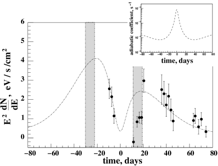
Figure 3: Main panel: The lightcurve of 1 TeV gamma-rays detected by HESS from PSR B1259-63/SS2883 (Aharonian et al., 2005). A reference lightcurve adopted for derivation of the time profile of nonradiative energy losses of electrons is also shown. The two vertical gray zones correspond to the position of the stellar disk. The somewhat lower flux of gamma-rays at $t\sim 15$ days after the periastron can be associated with the enhanced losses in the disk, and thus may cause more irregular profile of energy losses. Small panel: The reconstructed time profile of adiabatic energy loss rate derived for the reference TeV lightcurve shown in the main panel (see the text).

Figure 4: The energy losses for 1 TeV electrons versus the separation distance between the pulsar and the companion star. The solid line is for synchrotron losses for $B=0.1$G at periastron, and $B(D)\propto D^{-1}$; the dashed-dotted line is for IC losses for black body distribution of target photons with temperature $T=2.3\cdot 10^{4}$K diluted with coefficient $\kappa=(R_{\star}/2D)^{2}$, where $R_{\star}$ is the radius of the star. The dashed line corresponds to adiabatic losses for the reconstructed time-profile shown in Fig.3 (the small panel).

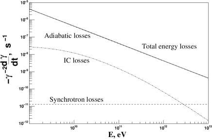
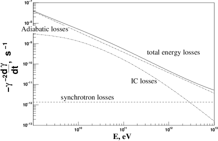
Figure 5: The energy loss rates calculated for two epochs: at periastron (top panel) and at $t=35$ days from periastron (bottom panel). The assumed parameters are the same as in Fig.4.

In Fig.6 we show lightcurves calculated for four different gamma-ray energies. The lightcurve for 1 TeV coincides, by definition, with the reference lightcurve shown in Fig.3. The lightcurves generally are similar what is explained by a dominance of adiabatic losses at all electron energies. At the same time the energy spectra of IC radiation at different energy bands are significantly different. Indeed, the dominance of adiabatic or energy-independent escape losses maintains the acceleration spectrum of electrons unchanged. Thus at energies $E\ll E_{\rm max}$, the gamma-rays produced in the Thompson regime ($E_{\gamma}\leq 10$ GeV) will have a power-law spectrum with photon index $(\alpha+1)/2$, while in the deep Klein-Nishina regime the spectrum will be proportional to $E_{\gamma}^{-(\alpha+1)}\ln E_{\gamma}$. This effect is seen in Fig.7, where we show the broadband spectral energy distribution (SED) of radiation at different epochs, consisting of synchrotron and IC components. In Fig. 8 we also show the gamma-ray spectra averaged over three periods of HESS observations in February, March and April 2004. Within the statistical and systematic uncertainties, the agreement with the fluxes reported by HESS is satisfactory (Aharonian et al., 2005).

For the adopted key parameters, in particular for the electron adiabatic loss rates shown in Figs. 4, 5, the gamma-ray fluxes are not sensitive to the magnetic field strength as long as it does not exceed 0.5 G. At the same time, the synchrotron flux is very sensitive to the B-field ($\propto B^{2}$). It is seen in Fig.7 that for the assumed magnetic field 0.1G the fluxes of synchrotron X-rays are significantly below $10^{-11}\rm\ erg/cm^{2}s$, thus they cannot explain the X-ray data (Chernyakova et al., 2006). On the other hand, assuming a specific value of magnetic field $B_{*}=0.45$G at periastron, one can increase the synchrotron X-ray flux to the observed level, and, at the same time keep the gamma-ray fluxes practically unchanged. Not that any significant (20 % or so) deviation from this value of the magnetic field would lead to the reduction of X-ray fluxes (for $B\leq B_{*}$), or gamma-ray fluxes (for $B\geq B_{*}$) below the observed flux levels. The X-ray lightcurve, calculated for the B-field dependence $B=0.45(D_{0}/D)$G, is shown Fig.9. While the calculated lightcurve is in reasonable agreement with observations around the periastron and at high separations (more than 200 days), it significantly exceeds the fluxes between 200 days to several days before periastron. This implies a much weaker magnetic field, and thus the synchrotron radiation fails to explain the X-ray emission. A more speculative explanation could be that, the energy release in nonthermal particles for this period is suppressed, e.g. due to the the interaction with the stellar outflow. If the X-ray and gamma-ray components are produced by the same electron population, this effect will have a similar impact on the gamma-ray lightcurve, namely it should suppress significantly the gamma-ray fluxes. However the lack of gamma-ray data for this period does not allow any conclusion in this regard.

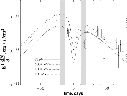
Figure 6: Gamma-rays lightcurves in the nonradiative loss dominated scenario are calculated for four different energies: $E_{\gamma}=1\,{\rm TeV}$ (solid line), $E_{\gamma}=0.5\,{\rm TeV}$ (dotted line), $E_{\gamma}=0.1\,{\rm TeV}$ (dash-dotted), $E_{\gamma}=10\,{\rm GeV}$ (dashed line). The HESS measurements (Aharonian et al., 2005) of 1 TeV gamma-ray fluxes are also shown. The model parameters are same as in Fig.4.

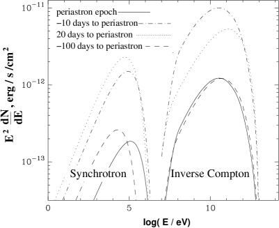
Figure 7: Broadband spectral energy distribution of synchrotron and IC components of radiation in the nonradiative loss dominated scenario. The spectra correspond to $t=-100$ days (dashed), -10 days (dash-dotted), 0 days (solid), +20 days (dotted line) epochs (periastron is at $t=0$). The model parameters are same as in Fig.4.

Figure 8: The time-averaged (over the HESS observation periods) TeV gamma-ray spectrum shown together with HESS measurements. The model parameters are same as in Fig.4

Figure 9: The X-ray lightcurve calculated for the adiabatic loss time-profile shown in Fig.3, and magnetic field strength $B=0.45(D/D_{0})^{-1}$ G. The point sets A1-A4, X1-X10, S1 correspond to ASCA (Hirayama et al., 1996), XMM-Newton (Chernyakova et al., 2006) and BeppoSAX (Chernyakova et al., 2006) observations, respectively. The open point corresponds to the 20-80 keV hard X-ray flux, $F_{\rm x}\sim 3\times 10^{-11}\ \rm erg/cm^{2}s$, as reported by the INTEGRAL team for the period 14.1-17.5 days after the periastron (Shaw et al., 2004).

4 Maximum energy of electrons

It is convenient to present the acceleration time of electrons in the following form:

$$t_{\rm acc}={\eta\,r_{\rm L}\over c}\approx 0.11\,E_{\rm TeV}\,B_{\rm G}^{-1}\,\eta\ {\rm s}\,,$$ (15)

where $r_{\rm L}$ is the Larmor radius, and $\eta$ is a dimensionless constant; $\eta=1$ corresponds to the maximum possible rate of acceleration allowed by classical electrodynamics. It is well known theoretically, that in case of nonrelativistic parallel shocks (with shock velocity $v$), $\eta>(c/v)^{2}\gg 1$ (see e.g. Pesses et al. (1982); Jokipii (2004); Aharonian et al. (2002)). Although this parameter is not consistently constrained by theory, $\eta$ can significantly exceed 1 even in the case of relativistic shocks. In the case when the energy losses of electron are dominated by synchrotron cooling, the maximum energy of the synchrotron radiation depends only on the $\eta$ parameter (see below for more details). Thus the measurements of the synchrotron radiation in the cutoff region can give us quite robust information about $\eta$. However, this simple relation does not work in the case of PSR B1259-63, at least for the models discussed here which assume that electrons are cooled via inverse Compton scattering or due to adiabatic losses. On the other hand, the spectral shape of fluxes of IC $\gamma$-rays, appear quite sensitive, especially at TeV energies, to the value of $\eta$. Thus if the suggested models describe the gamma-ray production scenarios correctly, we can derive information about $\eta$ from the comparison of model calculations with the observed gamma-ray spectra.

In Fig.10 we show characteristic acceleration times for 3 different values of $\eta=4\times 10^{3},\ 10^{3},\ 10^{2}$, together with synchrotron and Compton cooling timescales calculated for the epoch of the periastron assuming the magnetic field $B=0.05$ G. In Fig.10 the energy-independent escape time, which was assumed to be $10^{4}$ s, is also shown.

The maximum energy of electrons is determined from the balance of particle acceleration and loss rates, in Fig.10 this energy is defined by the intersection of curves corresponding to the acceleration and loss times. Because of essentially different energy dependences of characteristic energy loss times $t_{\rm syn}$, $t_{\rm IC}$ and $t_{\rm esc}$, the maximum electron energy is determined, depending on the value of $\eta$, by IC losses (a) or by escape (b) or by synchrotron losses (c) (see Fig.10).

If the electron energy losses are dominated by synchrotron cooling in the magnetic field $B_{\rm G}=B/1$ G with characteristic time

$$t_{\rm syn}\approx 400B_{G}^{-2}E_{\rm TeV}^{-1}\ {\rm s}\,,$$ (16)

the corresponding maximum energy of electrons is

$$E_{\rm e,max}\approx 2\,B_{\rm G}^{-1/2}\,\left(\eta\over 10^{3}\right)^{-1/2}~{}{\rm TeV}\,.$$ (17)

Note that in the case of $\eta={\rm const}$ the maximum energy of synchrotron photons does not depend on the magnetic field ($E_{\rm syn,max}\propto E_{\rm e,max}^{2}\ B$=const), but depends on $\eta$, namely $E_{\rm syn,max}\sim 100(\eta/10^{3})^{-1}\,{\rm keV}$. This relation contains unique information about the acceleration rate through the $\eta$ parameter.

Figure 10: The acceleration and cooling times of electrons at periastron. The solid line corresponds to the IC cooling time obtained with accurate numerical calculation; the thick solid line is the IC cooling time given by the Eq. (18); the dashed line corresponds to the synchrotron cooling time ($B=0.05\ {\rm G}$); the dashed-dotted line is the escape time; the dotted lines are acceleration times for $\eta=4\cdot 10^{3}$ (a),$\eta=10^{3}$ (b),$\eta=10^{2}$ (c).

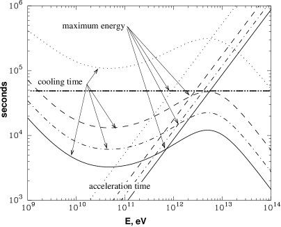
Figure 11: The acceleration and energy loss times of electrons of different epochs. The combined IC + synchrotron cooling times are calculated assuming $B_{0}=0.05\left(D_{\rm 0}/D\right)\ {\rm G}$ and $T=2.3\cdot 10^{4}\ {\rm K}$. The acceleration times are given by Eq.(15) assuming $\eta=4\cdot 10^{3}$. The horizontal dash-dot-dotted line corresponds to the $T_{\rm esc}=5\cdot 10^{4}{\rm s}$. The solid lines correspond to the periastron epoch; the dash-dotted lines to $\pm 10$ days; dashed lines to $\pm 20$days and dotted lines to $\pm 100$days. The maximum injection energy due to radiative cooling is determined by crossing of the same type lines. The maximum energy related to the electron escape is determined by crossing of an acceleration line with the escape line.

Figure 12: Maximum energy of electrons at the pulsar wind termination shock. The solid line corresponds to the cutoff energy caused by radiative cooling. The dashed line corresponds to the case of combined radiative and escape losses. The model parameters are same as in Fig.11.

In the regime when IC cooling dominates over the synchrotron cooling, the radiation cooling time is determined by

$$t_{\rm IC}\approx 7\cdot 10^{3}w_{0}^{-1}\ E_{\rm TeV}^{0.7}\ {\rm s}\,,$$ (18)

where $w_{0}$ is the energy density of the target photons in $\rm erg/cm^{3}$ units. In Fig.10 we show the accurate numerical calculation of the IC cooling time. It can be seen that above 1 TeV Eq.(18) provides quite accurate approximation of the IC cooling time.

The corresponding maximum energy of accelerated electrons is

$$E_{\rm e,max}\simeq 9\cdot 10^{5}\ \left(B_{\rm G}/w_{0}\right)^{3.3}\left(\eta\over 10^{3}\right)^{-3.3}\ {\rm TeV}\,.$$ (19)

This somewhat unusual dependence of $E_{\rm e,max}$ on the photon density $w_{0}$ is the result of IC scattering in deep Klein-Nishina regime. Obviously, in the Thomson regime $E_{\rm e,max}\propto\left(B_{\rm G}/w_{0}\right)^{1/2}\eta^{-1/2}$. The very strong dependence of $E_{\rm e,max}$ in Eq.(19) on three highly variable parameters, $B$, $w$ and $\eta$, allows variation of $E_{\rm e,max}$ in very broad limits. For example, for the $B\propto 1/D$ type dependence of the B-field, and assuming constant $\eta$, the increase of the separation between the compact object and the star by a factor of two would lead to the change of $E_{\rm e,max}$ by a factor of $2^{3.3}\simeq 10$, and correspondingly to dramatic variation of the flux of highest energy gamma-rays.

Finally, the escape of electrons may also have a strong impact on the variation of $E_{\rm e,max}$ depending on the position of the pulsar. Actually the effective escape of electrons from the acceleration site is somewhat shorter than the escape time. So in this case, ignoring the radiative energy losses of electrons and taking the upper limit for the escape from accelerator, one has

$$E_{\rm e,max}\simeq 9\,B_{\rm G}\left(T_{\rm esc}\over 10^{3}{\rm s}\right)\left(\eta\over 10^{3}\right)^{-1}\ {\rm TeV}\,,$$ (20)

where $T$ is the escape time of electrons.

Obviously, all relevant timescales depend on the pulsar position in the orbit, therefore the high energy cutoff in the spectrum of electrons is expected to be variable. As long as there no theoretical predictions for possible $\eta$ parameter dependence on physical conditions in the accelerator, in what follows we assume $\eta$ to be constant. In Fig.11 we show the radiation and acceleration timescales for different epochs – at periastron and $\pm 10,20,100$ days from the periastron. For the chosen model parameters, $B=0.05(D_{\rm 0}/D)$ G and $\eta=4\times 10^{3}$, the cutoff in the electron spectrum at the periastron is determined by IC losses, while at large separation distances the synchrotron and escape losses play the more important role in formation of the cutoff. This is demonstrated in Fig.12, where the high energy cutoff in the electron spectrum is shown as a function of epoch. Solid line corresponds to the case of radiation (IC and synchrotron) losses. In this case one expects significant reduction of the cutoff energy at epochs close to the periastron, where strong IC losses push the cutoff energy down to $\leq 1$ TeV. Far from the periastron, the cutoff energy can increase up to 10 TeV, unless the losses due to escape become dominant. The IC cooling time at the epoch with separation $D$ is $t_{\rm cool}\simeq 10^{3}{\rm s}(D/D_{0})^{2}$ s. Therefore, if the characteristic escape time is about $10^{4}$ s, the impact of particle escape becomes important for separations $D\geq 3D_{0}$. This effect is demonstrated in Fig.12 where (time and energy-independent) escape time $T_{\rm esc}=5\times 10^{4}$ s is assumed. One can see that for chosen model parameters the cutoff energy is a weak function of time with a local minimum ($\simeq 0.5$ TeV) at periastron, and two maxima ($\simeq 2.5$ TeV) at $\pm 20$ days.

It is important to note that the introduction of escape losses is crucial for explanation of the observed TeV lightcurve in this scenario. Indeed, while the reduction of the cutoff energy in the spectrum of electrons due to enhanced IC losses satisfactorily explains the minimum at the periastron, this would imply much higher fluxes at large separations in contrast to the HESS observations. The additional assumption that electrons suffer also significant escape losses ($T_{\rm esc}=5\times 10^{4}$ s) allows dramatic suppression of the gamma-ray fluxes beyond $|t|>20$ days (compare dashed and dot-dashed curves in Fig.2).

The impact of the variation of relative contributions of radiative and escape losses on the formation of the energy distributions of electrons is demonstrated in Fig.13. The corresponding lightcurves of inverse Compton gamma-rays at $E_{\gamma}=1$ TeV, 500 GeV, 100 GeV and 10 GeV, and 1-10 keV synchrotron photons are shown in Fig.14. For comparison the HESS measurements (Aharonian et al., 2005) of 1 TeV gamma-ray fluxes are also shown. The agreement of calculations with the HESS lightcurve is rather satisfactory except for somewhat higher predicted flux at the epoch of 2 weeks after the periastron which coincides with the pulsar passage through the stellar disk. In Fig.15 we compare the energy spectrum reported by HESS with the average TeV gamma-ray spectrum calculated for the period of the HESS observations in February 2004. Although it is possible to achieve a better agreement with the measurements, at this stage the attempt for a better spectral fit could be hardly justified given the statistical and systematic uncertainties of the measurements.

Through a variation of $E_{\rm e,max}$ the lightcurves at TeV and GeV energies can have quite different profiles. Namely, the TeV lightcurves have a clear minimum at periastron which is explained by the sub-TeV cutoff in the spectrum of accelerated electrons. At the same time this cutoff in the electron spectrum is still sufficiently high and therefore does not have a strong impact at GeV energies. Therefore the GeV lightcurves show their maximum a few days before the periastron . It is important to note that the significant drop of gamma-ray fluxes at large separations is due to the escape losses, otherwise one should expect rather constant flux with a weak maximum close to periastron. Also this model predicts different energy spectra of gamma-ray below 100 GeV at different epochs. Indeed, at large separations, when the escape losses dominate, the injection spectrum of electrons remains unchanged, therefore we expect noticeably harder gamma-ray spectra in the GeV energy band at epochs $|t|>20$ days (see Fig.16).

Remarkably, the calculated fluxes at GeV energies are well above the sensitivity of GLAST which makes this source a perfect target for future observations with GLAST. It should be noted, however, that the fluxes at GeV energies could be significantly suppressed due to a possible low energy cutoff in the acceleration spectrum of electrons. This is a standard assumption in the models of PWN, see e.g. Kennel & Coroniti (1984); Kirk et al. (1999).

In this scenario, the magnetic field energy density at the shock should be significantly less than the energy density of stellar photons. Thus, assuming the same strength of the magnetic field in the acceleration and radiation regions, one obtains quite low synchrotron fluxes (see Fig. 14). This would imply that the observed X-rays have non-synchrotron origin (e.g. IC origin; see (Chernyakova et al., 2006)). Another possibility is to assume that the magnetic field in the radiation region is somewhat higher than at the shock (note that that a similar situation takes place in the Crab nebula (Kennel & Coroniti, 1984)). In Fig.17 we show the lightcurve of 1-10 keV X-rays, assuming that in the radiation region the magnetic field is stronger by a factor of 8. If so, the synchrotron X-ray flux could achieve the observed flux level. In this scenario the X-ray and gamma-ray production regions are essentially different, although they could partly overlap. While the bulk of X-rays is formed in a magnetized region(s) far from the shock (where the electrons are accelerated), the IC gamma-rays come from more extended zones, which include also the site of particle acceleration. In Fig.17 we show also the 20-80 keV hard X-ray flux as reported by the INTEGRAL team for the 14.1-17.5 days after the periastron Shaw et al. (2004). Note that these days correspond to the minimum of the gamma-ray fluxes which we explain quantitatively by the passage of the pulsar through the disk, e.g. due to the the deficit of the target radiation field.

Figure 13: Electron energy distributions at different epochs ($0,\,\pm 10,\,\pm 20,\,\pm 100\,{\rm days}$ to periastron passage). The model parameters are same as in Fig.11.

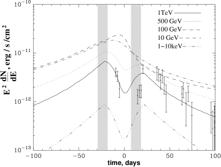
Figure 14: The gamma-ray lightcurves expected in the scenario of variation of the energy cutoff. The solid line: $E_{\gamma}=1\,{\rm TeV}$, the dotted line: $E_{\gamma}=0.5\,{\rm TeV}$, the dash-dotted line: $E_{\gamma}=0.1\,{\rm TeV}$, the dashed line: $E_{\gamma}=10\,{\rm GeV}$ and the dash-dot-dot-dotted line: $E_{\gamma}=1-10\,{\rm keV}$ (synchrotron). The model parameters are same as in Fig.11. The injection spectrum was assumed to be $Q(E_{\rm e})\propto E_{\rm e}^{-2}{\rm exp}\left(-E_{\rm e}/E_{\rm e,max}\right)$. The injection acceleration rate of electrons was assumed to be at level of 5% of the pulsar spindown luminosity. The HESS measurements (Aharonian et al., 2005) of 1 TeV gamma-ray fluxes are also shown. The vertical shadowed zones correspond to the stellar disk location.

Figure 15: The averaged spectrum of IC gamma-rays compeared with the spectrum measured by HESS during the period Feb. 2004. The model parameters are same as in Fig.14.

Figure 16: Gamma-ray spectra of synchrotron and IC radiation at -100 (the dashed line),-10 (the dotted-dashed line),0 (the solid line),+20 (the dotted line) days relative to the periastron passage. The model parameters are the same as in Fig.14.

Figure 17: The X-ray lightcurve calculated for the scenario with early sub TeV cutoff. At shock front the magnetic field was assumed to be $B_{0}=0.03\left(D_{\rm 0}/D\right)\ {\rm G}$, and in the emitting region to be higher by a factor of 10. The acceleration efficiency has value $\eta=4\times 10^{3}$. An orbital-dependent escape time was assumed to be $t_{\rm esc}=1.75\times 10^{4}\left(D/D_{\rm 0}\right)^{1/2}$ s. The point sets A1-A4, X1-X10, S1 correspond to ASCA (Hirayama et al., 1996), XMM-Newton (Chernyakova et al., 2006) and BeppoSAX (Chernyakova et al., 2006) observations, respectively. The open point corresponds to the 20-80 keV hard X-ray flux, $F_{\rm x}\sim 3\times 10^{-11}\ \rm erg/cm^{2}s$, as reported by the INTEGRAL team for the period 14.1-17.5 days after the periastron (Shaw et al., 2004).

5 Comptonization of the unshocked wind

While in the previous sections we tried to explain the observed modulation of TeV gamma-rays fluxes by energy losses of accelerated electrons at the termination of the wind, it is interesting to investigate whether one can relate the observed TeV lightcurve to the Compton losses of the kinetic energy of the bulk motion of the cold ultrarelativistic wind.

Generally this effect can be important in a binary system with a high luminosity companion star. Although the electrons in cold pulsar winds do not suffer synchrotron losses, a significant fraction of original kinetic energy of the bulk motion of the electron-positron wind could be radiated away due to Comptonization. Thus the power available for acceleration of electrons at termination of the wind depends on the position of the pulsar. Obviously, in this scenario we expect a minimum flux of gamma-rays closer to periastron. In other words, while in the previous section the modulation of the gamma-ray flux is linked to the $E_{\rm e,max}$, in this scenario the gamma-ray flux variation depends on the parameter $A$ characterizing the acceleration power of electrons given by Eq.(11).

According to the standard PWN model (Kennel & Coroniti, 1984) the isotropic cold electron-positron wind has a typical bulk motion Lorentz factor $\Gamma\propto 10^{4}-10^{6}$, thus the interaction of the wind electrons with starlight in the Klein-Nishina limit should lead to the formation of a narrow gamma-ray component with typical energy $\Gamma m_{e}c^{2}$. This effect also leads to the modulation of the bulk motion Lorentz factor as shown in Fig.18. The calculations in Fig.18 were performed for $L_{\rm star}=2.2\cdot 10^{38}{\rm erg/s}$ and different values of the initial Lorentz factor of the pulsar wind. Note that in the Thomson regime $t_{\rm cool}\propto\Gamma^{-1}$, i.e. the decrease of wind Lorentz factor leads to the increase of the cooling time. On the other hand, in the Klein-Nishina regime the cooling time increases with Lorentz factor as $t_{\rm cool}\propto\Gamma^{0.7}$. Therefore the maximum effect is achieved in the Thomson-to-Klein-Nishina transition region, i.e. around $\Gamma=10^{5}$.

As it follows from Fig.18, the initial Lorentz factor of the wind for $\Gamma_{\rm 0}=10^{5}$ is reduced by $40\%$ at periastron. Interestingly, minimum reduction of the initial Lorentz factor ($\sim 5\%$) happens around $t=\pm 20$ days (see in Fig.18). Since the kinetic energy of the wind radiated away due to the Comptonization is determined by the starlight density and the length of the unshocked wind $\Delta l=r_{\rm sh}$, the lightcurve is explained by the combination of two factors – dependence of the starlight density on the separation $D$, and the distance to the wind termination point (it is assumed that the gas density of the stellar wind decreases as $D^{2}$). Obviously, in the case of electron-positron pulsar wind, the kinetic energy of bulk motion of the wind, and consequently the rate of shock accelerated electrons have similar time behaviors: $A=A_{\rm 0}\Gamma(t)/\Gamma_{\rm 0}$, where $A_{\rm 0}$ characterizes the original power of the wind.

Although qualitatively this behavior agrees with the TeV lightcurve detected by HESS, the effect of reduction of the kinetic energy of the wind is not sufficient to explain quantitatively the observed TeV lightcurve. Indeed, the Comptonization of the wind can lead to the reduction of the energy flux of TeV gamma-rays at periastron by only a factor of $\leq 1.5$, while the HESS observations show more significant variation of the gamma-ray flux. Assuming somewhat larger, by a factor of two, luminosity of the optical star, one can get a better agreement with the observed TeV lightcurve. However, the range of luminosity of the star discussed in the literature favors a lower luminosity of the star (Tavani & Arons, 1997; Kirk et al., 1999). Therefore the effect of Comptonization of the pulsar wind cannot play, even for $\Gamma_{\rm 0}\sim 10^{5}$, a major role in the formation of the TeV lightcurve.

Even so, this effect cannot be ignored in the calculation of the overall gamma-radiation of the system. Namely the Comptonization of the ultrarelativistic pulsar wind unavoidably leads to an additional component of gamma-rays produced at the pretermination stage of the wind. Due to the inverse Compton scattering of monoenergetic electrons on target photons with narrow, e.g. Planckian distribution, we should expect a specific, especially for $\Gamma_{\rm 0}\geq 10^{5}$, line-type gamma-ray emission (Bogovalov & Aharonian, 2000; Ball & Kirk, 2000; Ball & Dodd, 2001). Ball & Kirk (2000) have calculated the IC radiation of the freely expanding wind, i.e. under assumption that the wind was not terminated. These calculations can be hardly applied for this system, since we see broad-band IC radiation of the shocked wind. As it was shown in the paper by Ball & Dodd (2001), such an assumption leads to significant (an order of magnitude) overestimation of the gamma-ray flux. Unfortunately in the paper by Ball & Dodd (2001) there are only calculations for one value of Lorentz factor $\Gamma=10^{6}$. To supply this gap we performed calculations for a number of probable Lorentz factors. The results of calculations of gamma-ray spectra of the unshocked wind are shown in Fig.19. Comparison of these calculations with the average energy spectrum of PSR B1259-63 measured by HESS excludes the initial Lorentz factor of the wind $\Gamma_{\rm 0}=10^{6}$. Otherwise, the flux of the Comptonized emission of the unshocked wind would exceed the observable flux even at apastron (see Fig.19). Due to the energy range of gamma-rays from this source available for HESS ($E\geq 300$ GeV), future observations unfortunately cannot significantly improve this limit. On the other hand, such studies can be performed by GLAST the sensitivity of which seems to be adequate, as is shown Fig.19, for a deep probe of the initial wind Lorentz factors of PSR B1259-63 within $10^{4}$ to $10^{6}$. Thus, GLAST has a unique potential to prove the current pulsar wind paradigm which assumes that the bulk of the spin-down luminosity of the pulsar is transformed to a cold wind with Lorentz factor exceeding $10^{4}$.

6 Summary

One of the recent exciting results of observational gamma-ray astronomy is the detection of TeV gamma-ray signal from the binary system PSR B1259-63/SS2883 (Aharonian et al., 2005). While the absolute fluxes and energy spectra of TeV emission detected by HESS can be explained quite well in the framework of inverse Compton model (Kirk et al., 1999), the observed TeV lightcurve appears to be significantly different from early predictions. This can be considered as an argument in favor of alternative (hadronic) models which relate the maximum in the TeV lightcurve observed after approximately three weeks of the periastron to the interaction of the pulsar wind with the stellar disk (Kawachi et al., 2004; Chernyakova et al., 2006). However, the hadronic models require a rather specific location of the stellar disk, which needs to be confirmed, since this assumption does not agree with the location of the stellar disk derived from the pulsed radio emission observations (Bogomazov, 2005).

The main objective of this paper is to show that the HESS results can be explained, under certain reasonable assumptions concerning the cooling of relativistic electrons, by inverse Compton scenarios of gamma-ray production in PSR B1259-63/SS2883. Namely, we study three different scenarios of formation of gamma-ray lightcurve in the binary system PSR B1259-63/SS2883 with an aim to explore whether one can explain the observed TeV lightcurve by electrons accelerated at the pulsar wind termination shock. The natural target for the inverse Compton scattering in such a system is the thermal radiation from the optical star. Since the basic parameters characterizing the system are well known, the predictions of gamma-ray fluxes at different epochs can be reduced to a calculation of the energy distribution of the relativistic electrons under certain assumptions concerning the acceleration spectrum of electrons and of both their nonradiative (adiabatic and escape) and radiative (Compton and synchrotron) energy loss origin. In particular, we demonstrate that the observed TeV lightcurve can be explained (i) by adiabatic losses which dominate over the entire trajectory of the pulsar with a significant increase towards periastron, or (ii) by the variation of the cutoff energy in the acceleration spectrum of electrons due to the modulation of rate of inverse Compton losses depending on the position of the pulsar relative to the companion star. Our models failed to explain the first four data points obtained just after periastron, what can be explained by a possible interaction with the Be star disk, which introduces additional physics not included in the presented model. Although we deal with a very complex system, we demonstrate that the observed TeV lightcurve can be naturally explained by the inverse Compton model under certain physically well justified assumptions. Unfortunately, the large systematic and statistical uncertainties, as well as the relatively narrow energy band of the available TeV data do not allow robust constraints on several key model parameters like the magnetic field, escape time, acceleration efficiency, etc. This also does not allow us to distinguish between different scenarios discussed above. In this regard, the future detailed observations both in MeV/GeV and TeV bands by GLAST and HESS closer to periastron, as well as at the epochs when the pulsar crosses the stellar disk, will provide strong insight into the nature of this enigmatic object. Equally important are the detailed observations of X-rays, e.g. with Chandra, XMM and Suzaku telescopes. The analysis of gamma and X-ray data obtained simultaneously should allow extraction of several key parameters characterizing the binary system.

Finally, although the Compton cooling of the unshocked electron-positron wind does have significant impact on the formation of the TeV lightcurve, the specific, line type gamma-radiation caused by the Comptonization of the cold ultrarelativistic wind should unavoidably appear either at GeV or TeV energies depending on the initial Lorentz factor of the wind. Detection of this component of gamma-radiation, in particular by GLAST, of the unshocked wind will provide unique information on the formation and dynamics of pulsar winds.

Figure 18: The time-evolution of the wind Lorentz factor just before the termination. The results are presented for the initial Lorentz factors $\Gamma_{\rm 0}=10^{5}$ (solid line), $\Gamma_{\rm 0}=10^{6}$ (dotted line) and for $\Gamma_{\rm 0}=10^{4}$ (dashed-dotted line) for the luminosity of the companion star $L_{\rm star}=2.2\cdot 10^{38}$ erg/s. Dashed line shows the time evolution of the wind Lorentz factor for $\Gamma_{\rm 0}=10^{5}$ calculated the luminosity of the companion star $L_{\rm star}=3.3\cdot 10^{37}$ erg/s.

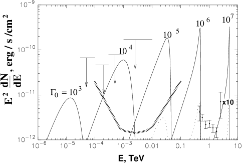
Figure 19: The energy spectra of gamma-rays due to the Comptonization of the unshocked wind at the periastron (solid lines) and apastron (dotted lines) are calculated for initial Lorentz factor $\Gamma_{\rm 0}=10^{3},10^{4},10^{5},10^{6}$ and $10^{7}$ (indicated at the curves). The luminosity of the companion star was assumed $L_{\rm star}=2.2\cdot 10^{38}$ erg/s. The experimental points correspond to the average energy spectrum measured by HESS within several weeks around the periastron, note that the last measurement was multiplied by a factor of 10. The upper limits in energy range 30MeV-3GeV correspond to the EGRET measurements (Tavani et al., 1996). The differential flux sensitivity of GLAST for a point source is also shown. The corresponding curve represents sensitivity for one-year all-sky survey taken from http://www-glast.slac.stanford.edu/software/IS/glast_lat_performance.htm. However, since gamma-ray fluxes can be effectively observed only at the epochs not far from the periastron, the typical available observation time by GLAST would be limited by $\Delta t\leq 3$ weeks. This implies that the minimum detectable gamma-ray flux of GLAST shown in the figure should be increased by a factor between $(1{\rm year}/\Delta t)^{1/2}\simeq 4$ and $16$ depending whether the sensitivity is determined by the background or by the gamma-ray photon statistics.

References

- Aharonian et al. (2002) Aharonian F., Belyanin A. A., Derishev E. V., Kocharovsky V. V., Kocharovsky V. V., 2002, PhysRevD, 66, 023005
- Aharonian et al. (2005) Aharonian F., et al., 2005, A&A, 442, 1
- Bogomazov (2005) Bogomazov A. I., 2005, Astronomy Reports, 49, 709
- Ball & Kirk (2000) Ball L., Kirk J., 2000, Astroparticle Physics, 12, 355
- Ball & Dodd (2001) Ball L., Dodd J., 2001, Publications of the Astronomical Society of Australia, 18, 98
- Bogovalov & Aharonian (2000) Bogovalov S., Aharonian F., 2000, MNRAS, 313, 504
- Bogovalov & Khangoulian (2002) Bogovalov S., Khangoulian D., 2002, MNRAS, 336, L53
- Bogovalov et al. (2007) Bogovalov S., Koldoba A.V. Ustyugova G.V., Khangulyan D., Aharonian F.A., 2007, in preparation
- Chernyakova et al. (2006) Chernyakova M., Neronov A., Lutovinov A., Rodriguez J., Johnston S., 2006, MNRAS, 367, 1201
- Dubus (2005) Dubus G., 2005, astro-ph/0509633
- Ginzburg & Syrovatskii (1964) Ginzburg V. L., Syrovatskii S. I.,1964, The Origin of Cosmic Rays. New York
- Harding & Gaisser (1990) Harding A. K., Gaisser T. K., 1990, ApJ, 358, 561
- Hirayama et al. (1996) Hirayama M., Nagase F., Tavani M., Kaspi V. M., Kawai N., Arons J., 1996, PASJ, 48, 833
- Johnston et al. (2005) Johnston S., Ball L., Wang N., Manchester R. N., 2005, MNRAS, 358, 1069
- Johnston et al. (1992) Johnston S., Manchester R. N., Lyne A. G., Bailes M., Kaspi V. M., Qiao G., D’Amico N., 1992, ApJ, 387, L37
- Jokipii (2004) Jokipii J.R., 1987, ApJ, 313, 842
- Kawachi et al. (2004) Kawachi A., et al., 2004, ApJ, 607, 949
- Kennel & Coroniti (1984) Kennel C., Coroniti F., 1984, ApJ, 283, 694
- Khangulyan & Aharonian (2005) Khangulyan D., Aharonian F., 2005, AIP Conference Proceedings, 745, 359
- Kirk et al. (1999) Kirk J., Ball L., Skjæraasen O., 1999, Astroparticle Physics, 10, 31
- Kirk et al. (2005) Kirk J., Ball L., Johnston S., 2005, astro-ph/0509901,astro-ph/0509899
- Pesses et al. (1982) Pesses M.E., Decker R.B., Armstrong T.P., 1982, SSRv, 32, 185
- Rees & Gunn (1974) Rees M. J., Gunn J. E., 1974, MNRAS, 167, 1
- Shaw et al. (2004) Shaw S. E., Chernyakova M., Rodriguez J., Walter R., Kretschmar P., Mereghetti S., 2004, A&A, 426, L33
- Tavani & Arons (1997) Tavani M., Arons J., 1997, ApJ, 477, 439
- Tavani et al. (1996) Tavani M., Grove J. E., Purcell W., et al., 1996, A&AS, 120, C221+
- Waters et al. (1988) Waters L.B.F.M., Taylor A.R., van den Heuvel E.P.J., Habets G.M.H.J., 1988, A & A, 198, 200