Stellar polytropes and Navarro-Frenk-White halo models: comparison with observations

Abstract

Motivated by the possible conflict between the Navarro-Frenk-White(NFW) model predictions for the dark matter contents of galactic systems and its correlation with baryonic surface density, we will explore an alternative paradigm for the description of dark matter halos. Such an alternative emerges from Tsallis’ non-extensive thermodynamics applied to self-gravitating systems and leads to the so-called “stellar polytrope” (SP) model. We consider that this could be a better approach to real structures rather than the isothermal model, given the fact that the first one takes into account the non-extensivity of energy and entropy present in these type of systems characterized by long-range interactions. We compare a halo based on the Navarro-Frenk-White (NFW) and one which follows the SP description. Analyzing the dark matter contents estimated by means of global physical parameters of galactic disks, obtained from a sample of actual galaxies, with the ones of the unobserved dark matter halos, we conclude that the SP model is favored over the NFW model in such a comparison.

, ,

keywords: dark matter, galaxy dynamics

1 Introduction

The standard statistical mechanical treatment for self–gravitational systems is provided by the micro-canonical ensemble, leading to a regime dominated by gravity and characterized by well known effects such as the non–extensive nature of energy and entropy, negative heat capacities and the so–called gravothermal instability. An alternative formalism that allows also non-extensive forms for entropy and energy under simplified assumptions, has been developed by Tsallis [1] and applied to self–gravitating systems [2, 3, 4] under the assumption of a kinetic theory treatment and a mean field approximation. As opposed to the Maxwell–Boltzmann distribution that follows as the equilibrium state associated with the usual Boltzmann–Gibbs entropy functional, the Tsallis’ functional yields as equilibrium state the “stellar polytrope”, characterized by a polytropic equation of state with index $n$ (see equation (2)). The stellar polytrope (SP) yields a Maxwell–Boltzmann distribution function (the isothermal sphere) in the limit $n\to\infty$. This index is related to the “non–extensivity” parameter $q$ of Tsallis entropy functional, so that the “extensivity” limit $q\to 1$ corresponds to the isothermal sphere.

Although the self–gravitating collisionless and virialized gas that makes up galactic halos is far from the state of gravothermal catastrophe, it is reasonable to assume that it is near some form of relaxation equilibrium characterized by non–extensive forms of entropy and energy. Admitting that the SP model follows from an idealized approach based on kinetic theory and an isotropic distribution function, it is interesting to verify empirically if the structural parameters of the halo gas can be adjusted to those of SPs, the equilibrium states under Tsallis’ formalism.

On the other hand, high precision N–body numerical simulations based on Cold Dark Matter (CDM) models, perhaps the most powerful method available for understanding gravitational clustering, lead to the famous results of Navarro, Frenk and White (NFW model) [5] that predicts density and velocity profiles which are roughly consistent with observations; however, it also predicts a cuspy behavior at the center of galaxies that is not observed in most of the rotation curves of dwarf and LSB galaxies [6, 7, 8, 9, 10, 11]. The significance of this discrepancy with observations is still under dispute, leading to various theoretical alternatives, either within the thermal paradigm (self–interacting [12] and/or “warm” [13] dark matter, made of lighter particles), or non–thermal dark matter models (with real [14, 15, 16, 17, 18] or complex [19] scalar fields, axions, etc), and none of these alternatives is free of controversy. However, for larger scales like galaxy clusters, the NFW paradigm is strongly supported by observations. A recent analysis [20] of ten nearby clusters using the X-ray satellite XMM-Newton has shown that clusters have indeed a cusped nature (see also [21] for a similar study using the Chandra satellite, and also [22] for a particular case study). Therefore, the CDM model of collision–less WIMPs remains as a viable model to account for dark matter in galactic halos, provided there is a mechanism to explain the discrepancies of this model with observations in the center of galaxies.

Since gravity is a long–range interaction and virialized self–gravitating systems are characterized by non–extensive forms of entropy and energy, it is reasonable to expect that the final configurations of halo structure predicted by N–body simulations must be, somehow, related with states of relaxation associated with non–extensive formulations of Statistical Mechanics; therefore, a comparison between the SP and NFW models is both, possible and interesting.

A theoretical comparison between the NFW model an the SP model is established in [23]. The aim of that paper was to verify which parameters of the stellar polytropes provide a suitable description of the halo that resembles the one that emerges from the NFW model. A convenient criterion was established for a best fit of the SP model to the NFW profiles followed by finding the stellar polytrope whose central density, $\rho_{c}$, central velocity dispersion, $\sigma_{c}$, and polytropic index, $n$, yields the same virial mass, total energy and maximal velocity of a given NFW halo model. Considering halo virial masses in the range $10^{12}-10^{15}\,M_{\odot}$, it was found that the best fit to NFW profiles at all scales is given by polytropic indices close to $n\approx 4.8$, leading to an empirical estimation of Tsallis non–extensive parameter: $q\approx 1.3$. We will describe with more detail the main idea and results of that work in the present paper.

The main purpose of our analysis is to make a dynamical analysis of two halo models, one based on the NFW paradigm, and other based on the SPs derived from Tsallis’ non–extensive thermodynamics, compare them and test both with observational results coming from a sample of disk galaxies.

The paper is organized as follows: in section II we provide the equilibrium equations of SPs and briefly summarize their connection to Tsallis’ non–extensive entropy formalism. In section III we discuss the dynamical variables of NFW halos, while in section IV we describe a procedure to compare a polytropic halo with an NFW one and obtain numerically the parameters that characterize such polytropic halos. Section V deals theoretically with the dynamical consequences due to the formation of the galactic disk within the halo. In section VI we describe the comparison with observations as well as the method we used to make such a comparison. A summary of our results is given in section VII.

2 Tsallis’ entropy and stellar polytropes

For a phase space given by $({\bf{r}},\,{\bf{p}})$, the kinetic theory entropy functional associated with Tsallis’ formalism is [2, 3, 4]:

$$S_{q}\ =\ -\frac{1}{q-1}\,\int{(f^{q}-f)\,{d}^{3}{\bf{r}}\,{d}^{3}{\bf{p}}},$$ (1)

where $f$ is the distribution function and $q>1$ is a real number. In the limit $q\rightarrow 1$, the functional (1) leads to the usual Boltzmann–Gibbs functional, corresponding to the isothermal sphere. The condition $\delta\,S_{q}=0$ leads to the distribution function that corresponds to the SP model characterized by the equation of state:

$$p\ =\ K_{n}\,\rho^{1+1/n},$$ (2)

where $K_{n}$ is a function of the polytropic index $n$, and can be expressed in terms of the central parameters:

$$K_{n}=\frac{{\sigma_{c}}^{2}}{{\rho_{c}}^{1/n}}$$ (3)

The polytropic index, $n$, is related to the Tsallis’ parameter $q>1$ by:

$$n\ =\ \frac{3}{2}+\frac{1}{q-1}$$ (4)

The standard approach for studying spherically symmetric hydrostatic equilibrium in stellar polytropes follows from inserting (2) into Poisson’s equation, leading to the well known Lane–Emden equation [24]:

$$\frac{1}{x^{2}}\,\frac{{d}}{{d}x}\left(x^{2}\,\frac{{d}\,\theta}{{d}x}\right)+\theta^{n}\ =\ 0,$$ (5)

with

$$\theta\ = \ \left(\frac{\rho}{\rho_{c}}\right)^{1/n},$$ (6)

$$x\ = \ \frac{r}{r_{0}},\quad r_{0}^{-2}\ =\ \frac{4\pi G\,\rho_{c}}{\sigma_{c}^{2}},\quad\sigma_{c}^{2}\ =\ \frac{p_{c}}{\rho_{c}},$$ (7)

$$G\ =\ 4.297\times 10^{-6}\,\frac{\left(\rm{km/sec}\right)^{2}}{\rm{M}_{\odot}/\rm{kpc}},$$ (8)

where, as mentioned above, $\sigma_{c}$ and $\rho_{c}$ are the central velocity dispersion and central mass density respectively; $G$ is the gravitational constant in appropriate units. Notice that the velocity dispersion is a measure of the kinetic temperature of the gas by means of the relation: $\sigma_{c}^{2}=k_{{}_{B}}\,T_{c}/m$, with $k_{{}_{B}}$ the Boltzmann’s constant, and that we are using a normalization for $r_{0}$, which differs from the usual one by a factor $1/(n+1)$. We find it more convenient to consider instead of equation (5) the following set of equivalent equilibrium equations:

$$\frac{\textrm{d}{\cal{M}}}{\textrm{d}x} =\ x^{2}\,{\cal{Z}},$$

$$\frac{\textrm{d}{\cal{Z}}}{\textrm{d}x} =\ -\frac{n}{n+1}\,\frac{{\cal{M}}\,{\cal{Z}}^{1-1/n}}{x^{2}},$$ (9)

where ${\cal{M}}$ and ${\cal{Z}}$ relate to $M,\,\rho$ (mass and mass density at radius $r$) by:

$${\cal{M}} =\ \frac{M}{4\pi\rho_{c}\,r_{0}^{3}},\qquad{\cal{Z}}\ =\ \frac{\rho}{\rho_{c}}$$ (10)

Notice that in the limit $n\to\infty$, equations (9) become the equilibrium equations of the isothermal sphere.

Once the system (9) has been integrated numerically, the velocity profile derived from the virial theorem takes the form:

$$V^{2}(x)\ =\ \sigma_{c}^{2}\,\frac{{\cal{M}}}{x}$$ (11)

The radial distance $r$ in kpc and enclosed mass $M(r)$ in solar masses are given (from equation (10)) in terms of $x$ and ${\cal{M}}$ by:

$$r/{\rm{kpc}} =\ 0.004220\,\,\frac{\sigma_{c}}{\rm{km/sec}}\,\,\left(\frac{\rm{M}_{\odot}/\rm{pc}^{3}}{\rho_{c}}\right)^{1/2}\,\,x,$$

$$M/{\rm{M}_{\odot}} =\ 944.97\,\,\left(\frac{\sigma_{c}}{\rm{km/sec}}\right)^{3}\,\,\left(\frac{\rm{M}_{\odot}/\rm{pc^{3}}}{\rho_{c}}\right)^{1/2}\,\,{\cal{M}}$$

Another important dynamical quantity is the total energy of the stellar polytrope [3]:

$$E\ = \ K+U$$

$$= \ \frac{3}{2}{\int_{0}}^{r}\,4\pi r^{2}P(r)\,dr-{\int_{0}}^{r}{dr\frac{GM(r)}{r}\frac{dM(r)}{dr}},$$

leading to

$$E_{poly}=-\,\frac{1}{n-5}\Big{[}\frac{3}{2}\,\frac{G\,M^{2}}{r}-\Big{(}\frac{\rho}{\rho_{c}}\Big{)}^{1/n}\,\sigma_{c}\Big{(}\frac{3}{2}(n+1)M_{v}-(n-2)4\,\pi\,{r}^{3}\,\rho_{v}\Big{)}\Big{]},$$ (14)

which must be evaluated at a fixed, but arbitrary, value of $r$ marking a cut–off scale.

Despite the valid general approach presented here it should be emphasized that there is confusion on the literature regarding the connection between $n$ and $q$ (equation (4)). The difference between different authors in this matter is mainly connected to the ambiguity on a proper definition of the one-particle distribution $f({\bf{r}},{\bf{p}})$ on terms of the probability $p({\bf{r}},{\bf{p}})$. In the “old” Tsallis’ formalism, the relation is $f\propto p$ which for self-gravitating systems reveals that the extremum state for the entropy gives: $f\propto(\Phi_{0}-v^{2}/2+\Phi({\bf{r}}))^{1/(q-1)}$ where $\Phi({\bf{r}})$ is the gravitational potential (see for example [3]). Such a distribution then leads to equation (4). The “new” Tsallis’ formalism introduced in [25] establishes the “choice”: $f\propto p^{q}$; under this definition the same treatment as in [3] leads to [26]: $f\propto(\Phi_{0}-v^{2}/2+\Phi({\bf{r}}))^{q/(q-1)}$ and then to $n=1/2+1/(1-q)$ (see also [27]). Another possibility exists for the connection between $n$ and $q$ using a different approach for the treatment of self-gravitating systems [28] which leads to $n=(5-3q)/2(1-q)$. There is still not a final word on which of these three possibilities is the most correct.

The first two are closely related by a so called duality transformation $q\leftrightarrow 1/q$ in the distribution function which seems to indicate that the thermodynamics properties in the new formalism ($f\propto p^{q}$) can be translated into the old formalism ($f\propto p$) at least for the microcanonical ensemble description (see [26]).

The differences between the third description and the first two are more complicated and out of the scope of this article; in [29], the authors present an analytical and numerical study for the velocity distribution functions of self-gravitating systems and they claim that it is in fact this third possibility the one that better agrees with their results.

Since there is yet no unique general agreement on which connection between $n$ and $q$, and the corresponding description leading to it, is the correct one, we will use the one presented in equation (4), considering that for the purposes of this work, the different expressions between $n$ and $q$ are just different ways of parameterizing the SPs and therefore, using one or the other will not lead to qualitative changes in the subsequent results. However it is important to be clear that this might not be true and a deeper analysis is needed to be sure about this issue; at least, as is clear for the different formulas connecting $n$ and $q$, the value for $q$ found and reported in Table 1 is absolutely dependent on our particular choice for the description leading to equation (4).

3 NFW halos

It is important to say that the NFW density profile [5] that we will describe in the present section and that will be used in this paper, is nowadays believed not to be the ultimate answer to the actual density profile of dark matter halos.

As was mentioned in the Introduction, the NFW density profile shows a cuspy behavior in the center, in fact, for this region, it has a power law dependence that goes as $\rho\sim r^{-1}$ whereas $\rho\sim r^{-3}$ for the outer regions; such features can easily be seen in equation (15). Recent numerical simulations have shown that different profiles can adjust better to the simulations (see for example [30] that propose a model where $\rho\sim r^{-0.75}$ in the center, see also [31] for a recent numerical analysis and the profile model discussed there). Also, semianalytical models [32, 33, 34] using a power law dependence for the phase space density: $\rho/\sigma^{3}\propto r^{-\alpha}$ (which holds for simulated dark matter halos), where $\sigma$ is the velocity dispersion, together with the Jeans equation have been established a model for a better understanding of the dynamics of halos; predicting in particular power law dependences of the density profile going as $\rho\sim r^{-0.8}$ in the central part and $\rho\sim r^{-3.44}$ in the external region.

However, to simplify our analysis we will use the NFW profile as a test model due to its well known analytical expressions, presented in the following paragraphs, leaving the analysis using more accurate models as a possible future work.

NFW numerical simulations yield the following expression for the density profile of virialized galactic halo structures [5, 35]:

$$\rho_{{}_{\mathrm{NFW}}}=\frac{\delta_{0}\,\rho_{0}}{y\,\left(1+y\right)^{2}},$$ (15)

where:

$$\delta_{0} =\frac{\Delta\,c_{0}^{3}}{3\left[\ln\,(1+c_{0})-c_{0}/(1+c_{0})\right]},$$ (16)

$$\rho_{0} =\rho_{\mathrm{crit}}\,\Omega_{0}\,h^{2}=253.8\,h^{2}\,\Omega_{0}\,\frac{M_{\odot}}{\rm{kpc}^{3}},$$ (17)

$$y =c_{0}\frac{r}{r_{v}},$$ (18)

where $\Omega_{0}$ is the ratio of the total density to the critical density of the Universe, being $1$ for a flat Universe. Notice that we are using a scale parameter, $y$, that is different from that of the stellar polytropes, $x$. The NFW virial radius, $r_{v}$, is given in terms of the virial mass, $M_{v}$, by the condition that average halo density is proportional to the cosmological density $\rho_{0}$:

$$\Delta\,\rho_{0}=\frac{3\,M_{v}}{4\,\pi\,r_{v}^{3}},$$ (19)

where $\Delta$ is a model–dependent numerical factor (for a $\Lambda$CDM model we have $\Delta\sim 100$ at $z=0$ [36]). We remark that this last relation between the mass and virial radius in terms of cosmological parameters, equation (19), is valid for any halo model. The concentration parameter $c_{0}$ can be expressed in terms of $M_{v}$ by [37, 38]:

$$c_{0}\approx 62.1\times\left(\frac{M_{v}\,h}{M_{\odot}}\right)^{-0.06}$$ (20)

hence all quantities depend on a single free parameter $M_{v}$. The mass function and circular velocity follow from (15):

$$M=4\,\pi\,\left(\frac{r_{v}}{c_{0}}\right)^{3}\,\delta_{0}\,\rho_{0}\,\left[\ln(1+y)-\frac{y}{1+y}\right],$$ (21)

$$V^{2}=4\,\pi\,G\,\delta_{0}\,\rho_{0}\,\left(\frac{r_{v}}{c_{0}}\right)^{2}\,\left[\frac{\ln(1+y)}{y}-\frac{1}{1+y}\right],$$ (22)

The total energy of the halo (evaluated at the virial radius) is given by [35]:

$$E_{{}_{\mathrm{NFW}}}=-\,G\,\frac{{M_{v}}^{2}}{2r_{v}}\,F_{0}$$ (23)

where $F_{0}$ has the approximate values:

$$F_{0}=\frac{2}{3}+\left(\frac{c_{0}}{21.5}\right)^{0.7}$$ (24)

4 SP and NFW comparison

In order to compare both halo models, we have to make various physically motivated assumptions. First, we want both models to describe a halo of the same size, but since the virial radius, $r_{v}$, is the natural “cut–off” length scale at which the halo can be treated as an isolated object in equilibrium, “same size” must mean same virial mass, $M_{v}$, by equation (19).

Second. Both models must have the same maximum value for the rotational velocity obtained from equations (11) and (22). This is a plausible assumption, as it is based on the Tully–Fisher relation, [39], a very well established result that has been tested successfully for galactic systems, showing a strong correlation between the total luminosity of a galaxy and its maximum rotational velocity. It can be shown that the Tully–Fisher relation has a cosmological origin [40, 41], associated with the primordial power spectrum of fluctuations (the so called “cosmological Tully-Fisher relation”), hence it is possible to translate the correlation between maximum rotational velocity and total luminosity to a correlation between maximum rotational velocity and total (i.e. virial) mass. Since, by construction we are assuming that the polytropic and NFW halos have the same $M_{v}$, their maximum rotational velocities must also coincide.

Our third assumption is that the polytropic and NFW halos, complying with the previous requirements, also have the same total energy evaluated at the cut–off scale $r=r_{v}$, which can easily be computed for each model. The main justification for this assumption follows from the fact that the total energy is a fixed quantity in the collapse and subsequent virialized equilibrium of dark matter halos [42].

Since all structural variables of the NFW halo depend only on the virial mass, once we provide a specific value for $M_{v}$ all variables become determined in terms of physical units by means of equations (20, 19 and 18). Polytropic halos, on the other hand, lack of a closed analytic expression for mass, velocity and density profiles. In this case, equations (9) (or (5)) yield numerical solutions for these profiles expressed in terms of the three free parameters $\left\{\rho_{c},\,\sigma_{c},\,n\right\}$. The comparison of these profiles with those of the NFW halos requires that we find explicit values of these free parameters, so that the conditions that we have outlined are met. Since we have selected three comparison criteria for three parameters, we have a mathematically consistent problem.

Following the guidelines described above, we proceed to compare NFW and polytropic halos for $M_{v}$ ranging from $10^{10}M_{\odot}$ up to $10^{15}M_{\odot}$. From the present comparison we find that the values for central density, $\rho_{c}$, of the polytropic halos are inversely proportional to $M_{v}$, while the values for the central velocity dispersion, $\sigma_{c}$, are directly proportional to it (this is expected, since $\sigma_{c}$ is a scale parameter in self–gravitating systems). The polytropic index, $n$, is almost constant for the selected range of $M_{v}$, showing a very small growth as $M_{v}$ increases. This implies the same qualitative behavior of the Tsallis parameter $q$: it is also almost constant and is slowly increasing as the virial mass grows. It is worthwhile mentioning that the proportionally term $K_{n}$ in the polytropic equation of state (2) shows a very noticeable change, rapidly growing as $M_{v}$ increases. All these results are displayed explicitly in Table 1. The comparison between both models in mass profiles, velocity profiles and density profiles is shown in figures 1, 2 and left panel of figure 3 respectively. SP and NFW models have both the same virial mass, $M_{v}=10^{12}\,M_{\odot}$. For other values of $M_{v}$ the mass, velocity and density profiles are qualitatively similar to the ones displayed in these figures.

The right panel of figure 3 shows the slope of the logarithmic density profile as a function of radius. On the figure we can see more easily how the slope changes form the inner to the outer regions of the halo. A generalized NFW profile like the one presented at the beginning of section 3 ([32, 33, 34]) will lie between the SP and NFW in this figure.

5 Including the galactic disk

So far we have analyzed only the global structure of the dark matter halo without considering the effects of the luminous galaxy within. If one wishes to test a given model with observational results, it is necessary to add the baryonic disk as a dynamical component of the model. We present some of the general ideas of a well known method used to establish a relation between the dynamical properties of disk galaxies formed within virialized halos, with the properties of the dark matter halo itself [35].

The initial conditions for the formation of the galactic disk are the following: an spherical halo model (SP, NFW, etc.) with a given mass, velocity and density profile; a total angular momentum $J$, total energy $E$ and a fraction $f_{d}$ of baryionic particles that will constitute the disk. In a dynamical context, the formation of disks inside dark matter halos can be well described with a model in which the halo responds adiabatically to the slow formation of the disk (due to energy dissipation of the baryonic particles). The method assumes that disk formation takes place in such a way that the final angular momentum of the disk, $J_{d}$, is a fraction of the total angular momentum of the halo: $J_{d}=j_{d}J$; this transfer of angular momentum is reasonable based on a hypothesis of adiabatic ensemble of the disk. $J_{d}$ is given by:

$$J_{d} = 2\pi\int_{0}^{r_{v}}rV_{d}(r)\Sigma_{d}(r)rdr,$$ (25)

$$= M_{d}h_{d}V_{v}\int_{0}^{r_{v}/h_{d}}e^{-u}u^{2}\frac{V_{c}(r)}{V_{v}}du,$$

where $u=r/h_{d}$, $V_{v}$ is the virial velocity and $V_{c}(r)$ is the total velocity profile(disk+halo).

The initial parameters of formation are given then by the scale quantities: $M_{v}$, $r_{v}$ or $V_{v}$ (halo) and $f_{d}$ (disk), and the dynamical quantities: $\lambda=\frac{J|E|^{-1/2}}{GM_{v}^{5/2}}$ (halo) and $j_{d}$ (disk).

The central hypothesis of the method is that the angular momentum of each particle in the halo, before and after disk formation, is conserved (due to the adiabatic assumption). Thus, a particle that is initially at a mean radius, $r_{i}$, ends up at mean radius, $r$, both related by:

$$M(r_{i})r_{i}=M_{f}(r)r,$$ (26)

The halo evolves by several dynamical processes which end up with the baryonic particles collapsing into a plane to form a disk. The dark matter particles remain in a spherically symmetric distribution, but they do feel a gravitational pull which makes each mass shell of the dark halo to shrink from its original position.

The galactic system is thus formed by two components: an spherically symmetric halo in virial equilibrium and a flattened disk with azimuthal symmetry on centrifugal equilibrium, both characterized by a radial density profile ($\rho(r)$ for the halo and $\Sigma(r)$ for the disk). The observed surface brightness profiles for disk galaxies favor an exponential form for the mass density of the baryonic disk: $\Sigma(r)=\Sigma_{d,0}e^{-r/h_{d}}$, where $h_{d}$ is a scale radius, and $\Sigma_{d,0}$ is the central surface density. For this distribution, the mass profile is:

$$M_{d}(r)=M_{d}\left[1-e^{r/h_{d}(1+r/h_{d})}\right],$$ (27)

where $M_{d}=2\pi\Sigma_{d,0}h_{d}^{2}$.

The rotation curve for a disk infinitely flat is given by Newtonian mechanics; a gravitational potential can be calculated using Poisson’s equation combined with the hypothesis of centrifugal equilibrium and the mass distribution of the disk (equation (27)); the calculation yields:

$$V_{d}^{2}(r)=4\pi G\Sigma_{d,0}h_{d}z^{2}\left[I_{0}(z)K_{0}(z)-I_{1}(z)K_{1}(z)\right],$$ (28)

where $z=r/2h_{d}$. Since real galaxies are not completely flat, we will correct the last formula according to an observational analysis [43], the correction diminish the value of $V_{d}$ in $5\%$ approximately.

The final mass distribution of matter $M_{f}$ is the sum of the dark matter inside the initial radius and the mass contributed by the disk:

$$M_{f}(r)=M_{d}(r)+M(r_{i})(1-f_{d}).$$ (29)

The velocity profile of the halo is given by the virial theorem:

$$V_{DM}^{2}=G\left(\frac{M_{f}(r)-M_{d}(r)}{r}\right).$$ (30)

The total rotational curve is the quadratic sum of disk and halo contributions. The mass distribution and the circular velocity of the disk, $M_{d}(r)$ and $V_{d}(r)$, depend on $h_{d}$ and $\Sigma_{d,0}$, see (27,28). The scale radius is obtained in terms of the initial conditions and the formula for the angular momentum of the disk (combining the expression for the parameter $\lambda$, with (25)):

$$h_{d}=\left(\frac{j_{d}}{f_{d}}\right)\lambda G^{1/2}M_{v}r_{v}^{1/2}|E|^{-1/2}f_{r}$$ (31)

where:

$$f_{r}\equiv\left[\int_{0}^{r_{v}/h_{d}}e^{-u}u^{2}\frac{V_{c}(h_{d}u)}{V_{v}}\right]^{-1}$$ (32)

The central surface density $\Sigma_{0,d}$ is obtained from the Freeman relation:

$$\Sigma_{0,d}=\frac{M_{d}}{2\pi h_{d}^{2}}=\frac{f_{d}M_{v}}{2\pi h_{d}^{2}}$$ (33)

To calculate the final mass distribution $M_{f}$ we need to find the initial radius of contraction, $r_{i}$, for each radius $r$, this is done by combining (26), (29) and (27) and solving the resulting transcendental equation. Once we obtain $M_{f}$, the velocity profile of the dark matter component can be calculated from equation (30).

It is important to mention that in the end both dynamical components (disk and halo) depend on the value of the scale radius, $h_{d}$, which turns out to depend implicitly on the final total circular velocity of the system (31,32), but $V_{c}$ also depends on $h_{d}$, so we need an iterative process to solve all the equations until a convergence for $h_{d}$ is obtained. Using the description presented, the model is complete and can be used to obtain total rotational curves from a set of initial conditions.

This method can be used for different mass profiles of the halo, and allows us to obtain results for different halo models; in particular we will use it for the NFW and SP models.

Both halo models which have been described before are characterized by isotropic velocity distributions for dark matter particles. However it is currently known that dark matter structures are actually anisotropic (see for example [33] and [44], see also [45], and [46]). Such models are parametrized by the quantity $\beta$, which is a measure of anisotropy: $\beta=1-\sigma_{\theta}/\sigma_{r}$, where $\sigma_{\theta}$ and $\sigma_{r}$ are the tangential and radial velocity dispersions. In the simplest case of isotropic orbits, $\sigma_{\theta}=\sigma_{r}$ and $\beta=0$. Analysis using numerical simulations in the past were not very clear about the value of $\beta$: in [47], $\beta\sim 0$ near the center and $\beta\sim 0.2$ at the virial radius whereas in [48] $\beta\sim 0.4$ at $r_{v}$. More recent works also suggest a universal relation between $\beta$ and the logarithmic slope of the radial density distribution [33, 44].

In order to include the effects of anisotropy in our analysis we would have to generalize the expressions for the different dynamical profiles, both for the NFW and SP models, using a given model for the radial dependence of $\beta$. Also, the model described for the adiabatic contraction of the halo due to formation of the disk in the halo would have to be generalized from circular to elliptical orbits. Such analysis is out of the scope of the present paper.

However, it is important to say that realistic models for dark matter halos should include the effects of anisotropy, then the fact that in the Tsallis’ formalism described here, the entropy is maximized for isotropic systems tells us that such a description can not be the final description of the nature of dark matter structures, our intention is more modest, to propose it as alternative approximation to real systems.

6 Comparison with observations

Now that we have described a dynamical model for the galactic system (disk+halo), we can use it to compare the NFW and SP models against observations coming from a sample of real disk galaxies.

The most direct approach would be to have observed rotation curves and surface brightness profiles (density distributions) for a representative sample of galaxies, then we could use a decomposition method to infer the components of the profile corresponding to dark and luminous matter for each galaxy in the sample; in this way, we would be able to analyze the radial distribution of each component and then, test both SP and NFW models to see which one fits better with the observations. However, as noticed by [37], such a sample which is also complete in galactic properties is hard to find. We are interested in a sample of galaxies that could be representative in the local Universe, i.e, that covers a wide range of luminosities, surface brightness and morphological types. Having such a sample will allow us to make an statistical analysis to test the SP and the NFW models. An alternative method to make the comparison we want is based in using global parameters of galaxies and the relations between them to explore the mass amounts of luminous and dark matter in disk galaxies. This method favors the statistical significance over precision. The approach used here will be on this direction, and we will use the outline described by [37] to make our analysis.

In [37], the authors compiled a sample with the desired characteristics: high quality surface photometry in the optical and near-infrared band (to obtain density profiles and integral luminosities), information about the rotation curves comes from the $H_{I}$ or $H_{\alpha}$ line-widths, and the total $H_{I}$ gas flux to take into account the gas contribution to the mass distribution. This sample is composed mainly by three subsamples described in [49, 50, 51, 52].

Some restrictions on the original samples were made in order to obtain the final one presented in [37]. One of them is about the relative inclination of the galaxies: the final sample of galaxies should not be highly nor slightly inclined. Otherwise either the surface brightness profiles in the former case, or the rotation velocities in the latter one, are not reliable. At the end, only galaxies with inclinations in the range of 35 to 80 degrees were considered. Galaxies with clear signs of interaction (mainly from the Verjeihen sample [51]) and with rotation curves which are still increasing at the last measured outer radius were excluded from the sample. Only some LSB galaxies present this feature. Fortunately, for most of the LSB galaxies in the sample the synthetic rotation curves are reported, so it was possible to perform such analysis in the exclusion criteria. The final sample consists of 78 galaxies and is not complete in a volume-limited sense, but is more or less homogeneous in the range of basic parameters: luminosity, surface brightness and morphological type. Dwarf galaxies were not included.

In order to have observations from the different samples as uniform as possible, the raw data for each one of them was taken an then corrected for the different factors that alter the actual measure of a given parameter. The total magnitudes were corrected for galactic extinction [53], $K-$correction [54], and internal extinction [55]. The surface brightness were corrected for galactic extinction, $K-$correction, cosmological surface brightness dimming, and inclination (geometrical and extinction effects). For the latter correction the authors in [37] followed the method presented in [56] and considered LSB galaxies as optically thin in all bands; they defined LSB galaxies as those whose disk central surface brightness in the $K-$band after correction is larger than 18.5 mag/arcsec². The 21 cm line-widths were corrected for broadening due to turbulent motions and for inclination, following [51].

The description of the sample, homogeneous data corrections and transformations from observational to physical parameters is carried on by the authors in [37] and the reader is refereed to their paper for more information about it.

With the information about the luminous disk structure parameters that we have from the sample (which can be used to obtain $h_{d}$ and $\Sigma_{0,d}$), the velocity component $V_{d}(r)$ can be calculated usin equation (28). A global quantity associated with the disk will be the maximum of $V_{d}(r)$:

$$V^{2}_{d,m}=4\pi GK\Sigma_{0,d}h_{d}$$ (34)

where $K\approx 0.193$; the maximum is located at $r\approx 2.2h_{d}$. The disk mass inside this radius is, according to equation (27): $M_{d}(2.2h_{d})=0.64M_{d}$. Thus, without introducing further assumptions, we may define the ratio of maximum disk velocity to maximum total (or dynamical) velocity, $V_{d,m}/V_{c,m}$, which is a global quantity that can be directly compared with theoretical predictions.

The $V_{d,m}/V_{c,m}$ ratio is not defined at a unique radius, but it can be related to the dynamical, total, disk mass ratio $M_{dyn}/M_{d}$, defined at an specific radius. In particular at radius $r_{m}$ where the total rotational curve reaches its maximum we have:

$$\left(\frac{M_{dyn}}{M_{d}}\right)_{r_{m}} = \frac{V_{c,m}^{2}r_{m}}{GM_{d}(r_{m})}$$ (35)

$$\approx \frac{V_{c,m}^{2}xh_{d}}{Gf_{L}2\pi\Sigma_{0,d}h_{d}^{2}}\propto\frac{x}{f_{L}}\left(\frac{V_{d,m}}{V_{c,m}}\right)^{-2},$$

where we have used the virial theorem, the Freeman relation and equation (34). The important assumption made is that $r_{m}$ is proportional to the scale radius: $r_{m}=xh_{d}$. In fact $x$ actually changes from galaxy to galaxy, depending on the disk surface density and halo mass distribution ($x\approx 2.2h_{d}$ for disk dominated galaxies, and $x>2.2$ for halo dominated galaxies); $f_{L}$ is the fraction of the total disk mass at $r_{m}$ and depends on the value of $x$ (when $x=2.2h_{d}$, $f_{L}=0.64$); however it was shown by [37] that $x$ changes slightly from galaxy to galaxy in the used sample (see figure 3a and 4a of [37]). The use of $V_{d,m}/V_{c,m}$ instead of $M_{dyn}/M_{d}$ is suitable because it can be obtained directly from observational parameters, without the assumptions needed to calculate $M_{dyn}/M_{d}$.

One of the principal results obtained in [37] is that the ratio $V_{d,m}/V_{c,m}$ correlates mainly with the disk surface density $\Sigma_{d}$. Therefore we will use this result to compare the NFW and the SP models with the observational results coming from the sample.

To do the comparison, we need to give the values for the free parameters of the models. $M_{v}$, $r_{v}$ and $V_{v}$ will be the same in both models, to account for same “size” of the halos, and they must have the same disk fraction $f_{d}$, meaning that the galactic disk inside the spherical halos will be of the same mass; we also require the same value for $j_{d}$, in this way the fraction of angular momentum of the disk to the halo will not depend, on a dynamical level, on the mass profile that the galactic system has before disk formation.

We will take $M_{v}=1\times 10^{12}M_{\odot}$, which is a characteristic value for the mass of dark matter halos, as the standard value for the virial mass. For simplicity, we will assume that $f_{d}$ and $j_{d}$ have the same values for all disks (that is, independent of $\lambda$); it turns out that in fact, the value of $f_{d}$ can not vary significantly from galaxy to galaxy, because this will predict larger scatter in the Tully-Fisher than the actually observed (Undergraduate Thesis [41]; an article which contains these an other results is currently in preparation). We will also use the standard assumption in modeling disk formation: $j_{d}/f_{d}=1$ [61, 35]; although it is unclear if this hypothesis is appropriate (it depends on the efficiency of disk formation) we will take it as valid for the purpose of this work, arguing that the change of this assumption does not change the statistical trend of the presented results. It has not been established an appropriate value for the disk fraction $f_{d}$. However, a plausible upper limit is the baryon fraction of the Universe as a whole ($f_{B}=\Omega_{B}/\Omega$), taking a Big Bang nucleosynthesis value for the baryonic density, $\Omega_{B}=0.015h^{-2}$ [62] gives an upper limit value on $f_{d}$ of 0.1 for a $\Lambda CDM$ cosmological model (see also [35]); however, the efficiency in forming the disk could be quite low, implying that $f_{d}$ could be substantially lower than $f_{B}$, this is confirmed by the results in [41] where an analysis on the scatter of the TF relation showed that $f_{d}$ has a numerical value even less than $0.05$. Taking into account these considerations we will take as average values for all galaxies in both models: $f_{d}=j_{d}=0.03$.

In figure 4 we show a plot of the ratio $V_{d,m}/V_{c,m}$ against $\Sigma_{d}$ for the described sample of galaxies (open circles). Despite the large scatter, an almost linear trend can be seen between this quantities, HSB (high surface brightness) galaxies (corresponding approximately to values of log$\Sigma_{d}$ greater than 2.5) have greater values of $V_{d,m}/V_{c,m}$ than LSB (low surface brightness) galaxies. This means that the luminous matter content is greater for HSB than for LSB galaxies. The shown picture is consistent with a well known result: LSB galaxies are dark matter dominated systems within optical radius.

The value of the graphic is that it allows us to bound statistically the possible values of the $V_{d,m}/V_{c,m}$ ratio that galaxies with a given surface density can have. As was proved by [37], the size of this range of values (associated with dispersion on the graphic) is due to different disk mass, i.e. different virial mass, color and morphological type that galaxies with the same $\Sigma_{d}$ have. As has been said, the value of $f_{d}$ can not vary significantly from galaxy to galaxy, nevertheless increasing $f_{d}$ will increase the value of $V_{d,m}/V_{c,m}$ and viceversa, as an example, taking an interval of 0.02 around the central value of $f_{d}=0.03$ changes the value of the ratio $V_{d,m}/V_{c,m}$ in 4% on average, being less for HSB galaxies and larger for LSBs. In figure 2 of [37] the result of varying $f_{d}$ can be seen explicitly. The observed dispersion seen in figure 4 mainly dependent on total disk mass and integral color (see figure 7a of [37]) has a cosmological origin which is explained with virial mass and concentration dispersion on the halos respectively (a galaxy formed inside a halo with a large value of the concentration parameter, will have an integral color redder than one formed inside a halo with a smaller value, an analogous conclusion is found for halos with different masses).

Figure 4 also shows clearly that NFW models can not reproduce at satisfaction the results obtained for the compiled sample without introducing unrealistic values for the virial mass or the concentration parameter. This is one of the results that lead us to the possibility of seeking an alternative to the NFW paradigm. The curves shown in figure 4 represent both models with average values for their respective parameter; it’s clear from the figure that the SP model follows in better agreement the average behavior of the observational sample than the NFW model. In terms of the parameters $\rho_{c}$, $\sigma_{c}$ and $n$ of the stellar polytrope model, the scatter of the observational results is explained in the same way as for the NFW model, $\rho_{c}$ takes the role of the concentration parameter and $\sigma_{c}$ the one corresponding to the virial mass (we found that the polytropic index $n$ is almost constant for virial masses in the range $10^{10}M_{\odot}$ to $10^{15}M_{\odot}$).

In [37], the same sample of observational data was also compared with results coming from self-consistent galaxy evolution models (see figure 3 of [37]). Such semi-numerical models were developed in [63, 64]; they follow the disk galaxy formation and evolution in a hierarchical $\Lambda$CDM scenario. These models include self-consistently halo formation and evolution, disk star formation and feedback processes, the gravitational dragging of the halo due to disk formation (where the adiabatic invariance is generalized to elliptical orbits), secular bulge formation and other evolution processes. The overall main difference is a small increase on the $V_{d,m}/V_{c,m}$ ratio in figure (4) for the more realistic models compared to the simpler model described in this paper (see section 3.2 of [37]), the difference is more notorious for HSB galaxies. It is remarkable then that despite the lack of real features like anisotropy, star formation and feedback, the simple (disk+halo) models presented above offer reasonable results compared to the evolutionary models, at least in what respect to figure 4, which is enough for the purpose of our work.

7 Conclusions

Motivated by the fact that stellar polytropes are the equilibrium states in Tsallis’ non–extensive entropy formalism, we have found the structural parameters of those stellar polytropes that allows us to compare them with NFW halos of virial masses in the range $10^{10}<M_{\textrm{\tiny{vir}}}/M_{\odot}<10^{15}$. The criteria for this comparison consists in demanding that the polytrope describes a halo having the same virial mass, virial radius, maximum rotational velocity and total energy as the NFW halo. These three conditions are sufficient to determine the three structural parameters $\left\{\rho_{c},\,\sigma_{c},\,n\right\}$ of the polytropic model; the results are displayed in Table 1.

We emphasize that the criteria which determine these polytropes are based on physically motivated assumptions: the virial radius and mass are the natural parameters characterizing the size of a given halo, same maximum velocity follows from the Tully–Fisher relation, while same total energy follows from the virilization process. As shown in Figure 1, the mass distribution of the polytrope grows much slower than that of the NFW halo up to a large radius (100 kpc) containing the core and the region where visible matter concentrates. Hence, as shown by Figure 2, the velocity profile of the polytrope is much less steep in the same region than that of the NFW halo. These features are consistent with the fact that NFW profiles predict more dark matter mass concentration than what is actually observed in a large sample of galaxies [65, 8, 37]. Also, as shown in the left panel of figure 3, the obtained polytropes have flat cores, very similar to the flat isothermal cores observed in LSB galaxies (as a contrast, the cuspy cores of NFW halos seem to be at odds with these observations [66, 67, 68], see also [65, 8]). This flat density core is a nice property, which combined with reasonable mass and velocity profiles, qualifies these polytropes as reasonable (albeit idealized) models of halo structures.

However, in spite of their nice theoretical properties (i.e. their connection to Tsallis’ formalism) and reasonable similarity with equivalent NFW halos, the stellar polytropes we have examined are very idealized configurations. Thus, we are not claiming that they provide a realistic description of halo structures. Instead, we suggest that their described features and their connection with Tsallis’ formalism might indicate that the latter could yield useful information to understand the evolution and virialization processes of dark matter. Although it is necessary to pursue this idea by means of more sophisticated methods, including the use of numerical simulations along the lines pioneered by [4], the simple approach we have presented has already given interesting results. For example, with respect to the parameter $q$( we recall that it is a free parameter of the Tsallis’ non-extensive thermodynamics and which has not been fixed for the cosmological case), in this work we were able to determine its behavior as a function of the virial mass, and turns out to be almost constant, with values around $q\approx 1.2$. This result could be used in other contexts where extended statistical mechanics is also applied [69]. We have also shown that the SP model is favored over the NFW model regarding the dark matter content in disk galaxies (within the optical radius) which is shown by the average behavior of the observational sample in figure 4. These results show that the NFW halo model can be enhanced with the use of alternative paradigms in statistical mechanics, which seems to solve a recurrent item which throws a shadow in such an excellent description as the NFW model is.

As mentioned, the results presented in this work show that a dark matter halo made out of particles which satisfy a polytropic equation of state, describes the halo in a way that is comparable with the description obtained from the NFW numerical simulations. Furthermore, our description has the advantage of not having a cuspy density profile near the galactic center. These results do not directly imply that dark matter halos obey a non-extensive entropy formalism. Further tests and experiments are needed in order to consider that such formalism is the one describing the dynamics of actual dark matter halos. At the moment, this idea is only a suggestion which is reinforced by our analysis.

Finally, we would like to address the possibility of a future analysis of the actual statistical mechanics treatment ruling the structure formation process of dark matter halos by using numerical simulations to obtain the equation of state obeyed by such systems at different times of their evolution and then determine towards which equilibrium state are they moving to. Thus allowing us to have a more reliable method to know whether or not the Tsallis’ formalism is appropriate for describing such self-gravitating systems.

References

Table 1: Parameters characterizing the polytropes while being compared to NFW halos

$\log_{10}(M_{v}/M_{\odot})$	$\rho_{c}\,[M_{\odot}/\rm{pc}^{3}]$	$\sigma_{c}\,[\rm{Km/s}]$	$n$	$q$	$K_{n}$	$v_{\rm{max}}\,[\rm{Km/s}]$	$r_{v}\,[\rm{kpc}]$
15	$3.7\times 10^{-4}$	$982$	$4.93$	$1.29$	$4873.4$	$1504$	$2606.2$
12	$7.5\times 10^{-4}$	$108$	$4.87$	$1.30$	$478.94$	$164$	$260.6$
11	$9.0\times 10^{-4}$	$52$	$4.83$	$1.30$	$221.82$	$79.1$	$120.9$
10	$1.2\times 10^{-3}$	$25$	$4.82$	$1.30$	$100.68$	$38.2$	$56.1$

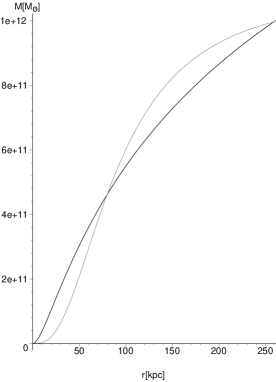
Figure 1: Mass profiles for a NFW halo with $M_{v}=10^{12}\,M_{\odot}$ and $r_{v}=260$ kpc (solid curve) and compared fit stellar polytrope (dashed curve).

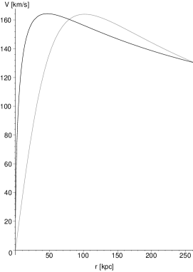
Figure 2: Velocity profiles for the same NFW halo of figure 1 (solid line) and its compared stellar polytrope (dashed curve).

Figure 3: In the left panel the density profiles for the same NFW halo of figures 1 and 2 (solid curve) and its compared stellar polytrope (dashed curve). In the right panel, the value for the slope of the logarithmic density profile is explicitly shown for different radii.

Figure 4: Luminous to total dark matter content vs central surface density; open circles correspond to observational data, the solid line represents the NFW model and the dashed one the SP model. Both models have $M_{v}=10^{12}M_{\odot}$.

References

- [1] Tsallis C, Nonextensive statistics: Theoretical, experimental and computational evidences and connections, 1999 Braz J Phys 29 1
- [2] Plastino A R and Plastino A, Stellar polytropes and Tsallis’ entropy, 1993 Physics Letters A 174 384
- [3] Taruya A and Sakagami M, Gravothermal Catastrophe and Generalized Entropy of Self-Gravitating Systems, 2002 Physica A 307 185 [cond-mat/0107494]
- [4] Taruya A and Sakagami M, Long-term Evolution of Stellar Self-Gravitating System away from the Thermal Equilibrium: connection with non-extensive statistics, 2003 Phys. Rev. Lett. 90 181101; See also Taruya A and Sakagami M, Self-gravitating Stellar Systems and Non-extensive Thermostatistics, 2004 Continuum Mechanics and Thermodynamics 16 279-292 [cond-mat/0310082]
- [5] Navarro J F, Frenk C S and White S D M, A Universal Density Profile from Hierarchical Clustering, 1997 ApJ 490 493 [astro-ph/9611107]
- [6] de Blok W J G, McGaugh S S, Rubin V C, High-resolution rotation curves of LSB galaxies: Mass Models, 2001 ApJ 122 2396 [astro-ph/0107366]
- [7] de Blok W J G, McGaugh S S, Bosma A and Rubin V C, Mass Density Profiles of LSB Galaxies, 2001 ApJ 552 L23 [astro-ph/0103102]
- [8] Binney J J and Evans N W, Cuspy Dark-Matter Haloes and the Galaxy, 2001 MNRAS 327 L27 [astro-ph/0108505]
- [9] Borriello A and Salucci P, The dark matter distribution in disc galaxies, 2001 MNRAS 323 285 [astro-ph/0001082]
- [10] Blais-Ouellette, Carignan C and Amram P, Multiwavelength Rotation Curves to Test Dark Halo Central Shapes, 2002 Preprint astro-ph/0203146
- [11] Bosma A, Invited review at IAU Symposium 220: Dark Matter in Galaxies, Sydney Australia, 21-25 Jul 2003, Preprint astro-ph/0312154
- [12] Spergel D N and Steinhardt P J, Observational evidence for self-interacting cold dark matter, 2000 Phys. Rev. Lett. 84 3760 [astro-ph/9909386]
- [13] Colin P, Avila-Reese V, and Valenzuela O, Substructure and halo density profiles in a Warm Dark Matter scenario, 2001 ASP Conference Series 230 p. 651-652 [astro-ph/0009317]
- [14] Guzmán F S and Matos T, Scalar fields as dark matter in spiral galaxies, 2000 Class. Quantum Grav. 17 L9 [gr-qc/9810028]
- [15] Matos T, Guzmán F S and Núñez D, Spherical Scalar Field Halo in Galaxies, 2000 Phys. Rev. D 62 061301 [astro-ph/0003398]
- [16] Matos T and Guzmán F S, On the Space Time of a Galaxy, 2001 Class. Quantum Grav. 18 5055 [gr-qc/0108027]
- [17] Matos T and Ureña-López L A, Scalar Field Dark Matter, Cross Section and Planck-Scale Physics, 2002 Phys. Lett. B 538 246 [astro-ph/0010226]
- [18] Guzmán F S and Ureña-López L A, Evolution of the Schrödinger–Newton system for a self–gravitating scalar field, 2004 Phys. Rev. D 69 124033
- [19] Ruffini R and Bonazzola S, Systems of selfgravitating particles in general relativity and the concept of equation of state, 1969 Phys. Rev. D 187 1767
- [20] Pointecouteau E, Arnaud M and Pratt G W, The structural and scaling properties of nearby galaxy clusters. I. The universal mass profile, 2005 A&A 435 1 [astro-ph/0501635]
- [21] Voigt L M and Fabian A C, Galaxy cluster mass profiles, 2006 Submitted to MNRAS [astro-ph/0602373]
- [22] Zappacosta L, Buote D A, Gastaldello F, Humphrey P J, Bullock J, Brighenti F and Mathews W, The absence of adiabatic contraction of the radial dark matter profile in the galaxy cluster a2589, 2006 Submitted to ApJ [astro-ph/0602613]
- [23] Cabral-Rosetti L G, Matos T, Nunez D, Sussman R and Zavala J, Empirical testing of Tsallis entropy in density profiles of galactic dark matter halos, 2006, in preparation.
- [24] Binney J and Tremaine S, Galactic dynamics, 1987, ed. Princeton University
- [25] Tsallis C, Mendes R S and Plastino A R, The role of constraints withing generalized nonextensive statistics, 1998 Physica A 261 534
- [26] Taruya A and Sakagami M, Gravothermal catastrophe and Tsallis’ generalized entropy of selfgravitating systems. 3. Equilibrium structure using normalized q values, 2003 Physica 322 285 [cond-mat/0211305]
- [27] Taruya A and Sakagami M, Antonov problem and quasi-equilibrium states in N-body system, 2005 MNRAS 364 990 [astro-ph/0509745]
- [28] Lima J A S and de Souza R E, Power law stellar distributions, 2005 Physica A 350 303 [astro-ph/0406404]
- [29] Hansen S H, Egli D, Hollenstein L and Salzmann C, Dark matter distribution function from non-extensive statistical mechanics, 2005 New Astronomy 10 379 [astro-ph/0407111]
- [30] Taylor J E and Navarro J F, The Phase-Space Density Profiles of Cold Dark Matter Halos, 2001 ApJ 563 483 [astro-ph/0104002]
- [31] Stoehr, F, Circular velocity profiles of dark matter haloes, 2006 MNRAS 365 147
- [32] Austin C G, Williams L L R, Barnes E I, Babul A and Dalcanton J J, Semianalytical Dark Matter Halos and the Jeans Equation, 2005 ApJ 634 756 [astro-ph/050657]
- [33] Dehnen W and McLaughlin D, Dynamical insight into dark-matter haloes, 2005 MNRAS 363 1057 [astro-ph/0506528]
- [34] Hansen s H and Stadel J, The velocity anisotropy - density slope relation, 2005 [astro-ph/0510656]
- [35] Mo H J, Mao S and White S D M, The Formation of Galactic Disks, 1998 MNRAS 295 319 [astro-ph/9707093]
- [36] Lokas E L and Hoffman Y, Nonlinear evolution of spherical perturbation in a non-flat Universe with cosmological constant, 2001 Preprint astro-ph/0108283. See also Lokas E L, Structure formation in the quintessential Universe, 2001 Acta Phys.Polon. B32 3643
- [37] Zavala J, Avila-Reese V, Hernández-Toledo H and Firmani C, The luminous and dark matter content of disk galaxies, 2003 A&A 412 633 [astro-ph/0305516]
- [38] Eke V R, Navarro J F and Steinmetz M, The Power Spectrum Dependence of Dark Matter Halo Concentrations, 2001 ApJ 554 114 [astro-ph/0012337]
- [39] Tully R B and Fisher J R, A new method of determining distances to galaxies, 1977 A&A 54 661, see also Colin P, Avila-Reese V and Valenzuela O, Substructure and halo density profiles in a Warm Dark Matter Cosmology, 2000 ApJ 542 622 [astro-ph/0004115]
- [40] Steinmetz, M and Navarro J F, The Cosmological Origin of the Tully-Fisher Relation, 1999 ApJ 513 555 [astro-ph/9808076]
- [41] Zavala J, El plano fundamental luminoso y bariónico de las galaxias de disco, 2003, Undergraduate thesis, UNAM.
- [42] Padmanabhan T, Structure formation in the universe, 1993, Cambridge University Press.
- [43] Burlak A N, Gubina V A and Tyurina N V, Allowance for the effect of finite thickness of galactic disks on the circular rotation velocity, 1997 Astro. Lett 23 522
- [44] Hansen S H, Moore B, A universal density slope - velocity anisotropy relation for relaxed structures, 2006 New Astronomy 11 333 [astro-ph/0411473]
- [45] Matos T, Nunez D and Sussman R A, The Spacetime associated with galactic dark matter halos, Gen. Rel. Grav., 37 769 [astro-ph/0402157]
- [46] Lokas E L and Mamon G A, Properties of spherical galaxies and clusters with an nfw density profile, 2001 MNRAS 321 155 [astro-ph/0002395]
- [47] Cole S and Lacey C G, The Structure of dark matter halos in hierarchical clustering models, 1996 MNRAS 281 716 [astro-ph/9510147]
- [48] Huss A, Jain B and Steinmetz M, The Formation and evolution of clusters of galaxies in different cosmologies, 1999 MNRAS 308 1011 [astro-ph/9703014]
- [49] de Jong R S and Van der Kruit P C, Near-infrared and optical broadband surface photometry of 86 face-on disk dominated galaxies. I. Selection, observations and data reduction, 1994 A&ASS 106 451
- [50] de Jong R S, Near-infrared and optical broadband surface photometry of 86 face-on disk dominated galaxies. III. The statistics of the disk and bulge parameters, 1996 A&A 313 45 [astro-ph/9601005]
- [51] Verheijen M W A and Sancisi R, The Ursa Major Cluster of Galaxies. IV : HI synthesis observations, 2001 A&A 370 765 [astro-ph/0101404]
- [52] Bell E, Barnaby D, Bower R G, de Jong R S, Harper Jr. D A, Hereld M, Loewenstein R F and Rauscher BJ, The star formation histories of low surface brightness galaxies, 2000 MNRAS 312 470 [astro-ph/9909401]
- [53] Schlegel D J, Finkbeiner D P and Davis M, Maps of Dust Infrared Emission for Use in Estimation of Reddening and Cosmic Microwave Background Radiation Foregrounds, 1998 ApJ 500 525 [astro-ph/9710327]
- [54] Poggianti B M, K and evolutionary corrections from UV to IR, 1997 A&ASS 122 399 [astro-ph/9608029]
- [55] Tully R B, Pierce M J, Huang J, Saunders W, Verheijen M A W and Witchalls P L, Global Extinction in Spiral Galaxies, 1998 AJ 115 2264 [astro-ph/9802247]
- [56] Verheijen M A W, PhD Theses, Groningen University, 1997
- [57] Karachentsev I D, Scatter of SC Galaxies in the Tully-Fisher Diagram and the Dark Matter Problem, 1991 SvAL 17 367
- [58] Salucci P and Borriello A, The Distribution of Dark Matter in Galaxies: Constant-Density Dark Halos Envelope the Stellar Disks, 2001 in ”Proceedings of the International Conference DARK 2000”, Heidelberg, Germany, p.12
- [59] Salucci P and Persic M, Maximal Halos in High-Luminosity Spiral Galaxies, 1999 A&A 351 442 [astro-ph/9903432]
- [60] Salucci P, Ashman K M and Persic M, The dark matter content of spiral galaxies, 1991 ApJ 379 89
- [61] Fall S M and Efstathiou G, Formation and rotation of disc galaxies with haloes, 1980 MNRAS 193 189
- [62] Walker T P, Steigman G, Kang H S, Schramm D M and Olive K A, Primordial nucleosynthesis redux, 1991 ApJ 376 51
- [63] Avila-Reese, V, Firmani C an Hernández X, On the Formation and Evolution of Disk Galaxies: Cosmological Initial Conditions and the Gravitational Collapse, 1998 ApJ 505 37
- [64] Avila-Reese, V and Firmani C, Properties of Disk Galaxies in a Hierarchical Formation Scenario, 200 RevMexAA 36 23 [astro-ph/0001403]
- [65] McGaugh S S, Rubin V C and de Blok W J G, High-Resolution Rotation Curves of Low Surface Brightness Galaxies. I. Data, 2001 ApJ 122 2381 [astro-ph/0107326]
- [66] Moore B, The Nature Of Dark Matter, 1994 Nature 370 629 [astro-ph/9402009]
- [67] Flores R and Primack J P, Observational and Theoretical Constraints on Singular Dark Matter Halos, 1994 ApJ 427 L1 [astro-ph/9402004]
- [68] Burkert A, The structure of dark matter halos. Observation versus theory, Aspects of Dark Matter in Astro-and Particle Physics (ed. Klapdor-Kleingrothaus H V and Ramachers Y), 1997 Preprint astro-ph/9703057
- [69] Tsallis C, Nonextensive Statistical Mechanics and its Applications, 2001, (Eds. Abe S and Okamoto, Y. Springer, Berlin, 2001)