Cosmological Simulations of Intergalactic Medium Enrichment from Galactic Outflows

Abstract

We investigate models of self-consistent chemical enrichment of the intergalactic medium (IGM) from $z=6.0\rightarrow 1.5$, based on hydrodynamic simulations of structure formation that explicitly incorporate outflows from star forming galaxies. Our main result is that outflow parameterizations derived from observations of local starburst galaxies, in particular momentum-driven wind scenarios, provide the best agreement with observations of C iv absorption at $z\sim 2-5$. Such models sufficiently enrich the high-$z$ IGM to produce a global mass density of C iv absorbers that is relatively invariant from $z=5.5\rightarrow 1.5$, in agreement with observations. This occurs despite continual IGM enrichment causing an increase in volume-averaged metallicity by $\sim\times 5-10$ over this redshift range, because energy input accompanying the enriching outflows causes a drop in the global ionization fraction of C iv. Comparisons to observed C iv column density and linewidth distributions and C iv-based pixel optical depth ratios provide significant constraints on wind models. Our best-fitting outflow models show mean IGM temperatures only slightly above our no-outflow case, metal filling factors of just a few percent with volume-weighted metallicities around $10^{-3}$ at $z\sim 3$, significant amounts of collisionally-ionized C iv absorption, and a metallicity-density relationship that rises rapidly at low overdensities and flattens at higher ones. In general, we find that outflow speeds must be high enough to enrich the low-density IGM at early times but low enough not to overheat it, and concurrently must significantly suppress early star formation while still producing enough early metals. It is therefore non-trivial that locally-calibrated momentum-driven wind scenarios naturally yield the desired strength and evolution of outflows, and suggest that such models represent a significant step towards understanding the impact of galactic outflows on galaxies and the IGM across cosmic time.

1 Introduction

The intergalactic medium (IGM) contains the majority of the Universe’s baryons (, 2001) and its largest structures, yet paradoxically can typically only be painstakingly observed in absorption against a background source. The marriage of high-resolution Echelle spectroscopy on 8-10m class telescopes with cosmological hydrodynamic simulations in the last decade has led to the understanding that the Lyman-$\alpha$ forest arises from highly-photoionized H i tracing fluctuations in the underlying IGM density in the so-called Fluctuating Gunn-Peterson Approximation (, 1998). This ionization state of the absorbing gas is governed by a balance between photo-ionizational heating due to the metagalactic UV background and adiabatic cooling from Hubble expansion, yielding a tight density-temperature relation known as the IGM equation of state (, 1997).

A surprising discovery was that the diffuse IGM is enriched with metals, seen as C iv, Si iv, and O vi absorption lines in quasar spectra. Despite our understanding of H i absorption, the origin of these metals far from sites of star formation remains puzzling. Currently the leading candidate for enriching the IGM is supernova-driven outflows, because dynamical disruption of galaxies is too inefficient (, 2001, see also Figure 10). Understanding such galactic feedback processes is crucial for developing a complete theory of galaxy formation and evolution (, 1986), as observations such as the shallow faint-end slope of the galaxy stellar mass function (, 2001) versus the halo mass function (, 2001), the galaxy mass-metallicity relation (, 2004, 2006), and the overproduction of stars in the Universe in models without feedback (, 2001, 2003b) indicate that outflows significantly affect galaxy properties.

Observations of metal abundance in various ions that trace different densities can quantify the metallicity-density relation in the IGM (, 1998), thereby constraining the nature of the enriching outflows. Early results from Keck’s High Resolution Echelle Spectrograph (HIRES) constrained typical IGM metallicities as traced by C iv to be $-3\la$[C/H]$\la-2$ (, 1996, 1998). Subsequent observations by (2001), (2003) (hereafter S03), and (2005) further showed that C iv absorption evolves very little from $z\sim 5\rightarrow 2$, which is surprising considering that the vast majority of stars in the Universe form at $z<5$. These results have been interpreted as implying early enrichment by primeval galaxies and/or Population III stars at $z>6$, where physical distances are small and shallow potential wells allow winds to distribute metals over large comoving volumes (, 2002). In contrast, (2003, 2005) observe enhanced C iv and O vi absorption in the vicinity of galaxies at $z\sim 2-3$, suggesting that enrichment is ongoing at lower redshifts in the form of superwinds from Lyman-break galaxies (, 2001, 2003). (2005) counter this by showing that such strong correlations can arise from metals ejected from dwarf galaxies between $z\approx 6-12$, because outflows from highly biased early galaxies should lie in highly overdense regions at lower redshifts. Hence the sources and epoch of IGM enrichment remain controversial.

Recent observations of local starbursts have provided new insights into the nature and impact of supernova-driven winds. Observations of dwarf starbursts and luminous infrared galaxies generally find outflows when detectable (, 2005, 2005), observed as blueshifted Na i absorption arising from cold clumps entrained in hot metal-rich outflowing gas. While earlier data showed little trend of outflow properties with host galaxy properties (, 1999, 2000), these more recent data suggest that massive galaxies with higher star formation rates (SFR’s) drive faster and more energetic winds. It is of particular interest here that recent data exhibit trends that are broadly consistent with theoretical expectations for momentum-driven (or radiation-driven) winds (, 2005, 2005), thereby providing for the first time some intuition on the physical mechanisms that drive outflows. In such a model, radiation from young stars impinges on dust in the outflow, which then couples to the gas and propels matter out of the galaxy (, 2005). This is somewhat different than the canonical scenario where the overpressure from local ISM heating causes a bubble that eventually bursts out of the galaxy (, 2004, e.g.). An advantage of momentum-driven winds is that, unlike heat, momentum cannot be radiated away, and hence can plausibly drive winds over large distances.

For our purposes, such scenarios for outflows provide a physically and observationally-motivated model connecting wind properties with host galaxy properties, which we can exploit in order to understand the global impact of outflows on the IGM across cosmic time. Doing so requires modeling large-scale outflows within the context of hierarchical structure formation. This is the main focus of this paper.

In this paper we explore the impact of various feedback mechanisms on IGM metallicity using cosmological hydrodynamic simulations, based on an explicit implementation of superwind feedback pioneered by (2003b) (hereafter SH03). Our simulations also include metal-line cooling, which significantly affects the temperature structure of metal-enriched IGM (, 2005). Our goal here is to construct an enrichment model that can reproduce both the metal-line observations of the IGM as well as the star formation history of the universe. We focus primarily on C iv absorption line observations between $z=1.5-6.0$ since this species is the cleanest tracer of IGM metallicity observable over this redshift range (, 1996, 1998).

This paper is organized as follows. §2 discusses the simulations including the modifications we made to Gadget-2, the various feedback models we run, and the generation of simulated spectra. §3 gives an overview of the global IGM physical properties in our suite of outflow simulations, while §4 discusses the physical characteristics of IGM metals and C iv absorbers. §5 compares our findings to observations analyzed by Voigt profile fitting of lines and the Pixel Optical Depth (POD) method. In §6 we show that our results are robust against the effects of numerical resolution. We present our conclusions in §7.

2 Simulations

2.1 Hydrodynamic Simulations of Structure Formation

We employ the N-body+hydrodynamic code Gadget-2 (, 2005), which uses a tree-particle-mesh data structure to efficiently compute gravitational forces on a system of particles, along with an entropy-conservative formulation of Smoothed Particle Hydrodynamics (SPH; , 2002) to model the pressure forces and shocks in the gaseous component. The code is fully adaptive in space and time, enabling simulations with large dynamic range crucial for studying galaxies together with large-scale structure.

Additionally, Gadget-2 models a number of physical processes important for the formation of galaxies. Star formation is modeled using a subgrid recipe in which each gas particle above a critical density where fragmentation becomes possible (calculated from the thermal Jeans mass based on the local cooling rate) is treated as a set of cold clouds embedded in a warm ionized medium, similar to the interstellar medium of our own Galaxy. The processes of evaporation and condensation are followed analytically within each particle using the formalism of (1977). Stars are allowed to form in the cold clouds at a rate proportional to its density squared. This produces a disk surface density-star formation rate relationship that is in agreement with the relation observed by (1998), when a single free parameter, the star formation timescale, is set to 2 Gyr (, 2003a). Feedback energy from Type II supernovae is then added to the hot phase of the ISM, using an instantaneous recycling approximation. SH03 found that the multi-phase model produces self-regulated star formation that does not suffer from runaway star formation with increasing resolution, as seen in previous simulations (, 2001, 2001). However, the converged star formation rate was still found to be too high when compared with observations, motivating SH03 to include galactic outflows as we describe in §2.3.

Photo-ionization heating is incorporated based on a spatially-uniform ultraviolet background taken from (2001), described in detail in §2.6. Gadget-2 also includes radiative cooling. In the simulations run by SH03, the cooling rates were computed assuming primordial composition with 76% hydrogen by mass. In §2.2 we describe improvements to the cooling module and extend it to include metal-line cooling.

Gadget-2 tracks the metallicity of gas and stellar particles. Gas particles that are eligible to form stars continually enrich themselves with metals based on an assumption of instantaneous recycling and using a yield of 0.02 (i.e. solar metallicity). This yield is roughly what one would expect using supernova yields from (1995) in a Chabrier IMF. When a particle is converted into a star (which happens in two stages, such that each star particle has half the mass of its original gas particle), then the star particle inherits the metallicity of its parent gas particle at the time of conversion.

2.2 Radiative Cooling With Metal Lines

In the simulations of SH03, cooling is done using an implicit scheme wherein the cooling timestep is the same as the hydrodynamical timestep as set by the Courant condition (, 2002). While in most cases this is a stable and accurate method, in dense regions surrounding galaxies the cooling time can be considerably shorter than the sound crossing time, but still not so rapid so that the particle reaches thermal equilibrium within such a time. Since the implicit method uses the cooling rate at the end of the timestep to evolve the thermal energy over the entire timestep, it can give inaccurate answers in regions where the slope of the cooling curve is varying rapidly. This happens at moderately high densities, and at temperatures $\sim 10^{4.5}-10^{5.5}$ K (see , 1996, for some examples of cooling curves).

In order to handle this regime better, we have modified Gadget-2 to implement a scheme to follow cooling on the cooling timescale. As with (2003a), we assume that the particle’s density and non-radiative rate of change of thermal energy remain fixed during the dynamical timestep; these assumptions are of course not valid in detail, but are made to facilitate ease of computation. We also continue to assume ionization equilibrium at all times, although the algorithm we have implemented makes it easier to follow non-equilibrium evolution; non-equilibrium effects are not expected to be important in the moderately overdense IGM that will be the focus of this paper.

We compute the cooling time as

$$t_{\rm cool}=\epsilon_{\rm cool}{u\over du/dt},$$ (1)

where $u$ is the thermal energy, $du/dt$ is the rate of change of thermal energy, and $\epsilon_{\rm cool}$ is a tolerance factor that we set to 0.002. This choice means that in a single cooling timestep a particle cannot cool away more than 0.2% of its thermal energy. We further limit the cooling timescale such that it cannot be less than 0.2% the dynamical timescale, so a particle can take up to 500 cooling timesteps for each dynamical timestep. The value of this tolerance parameter was chosen based on numerous tests on individual particles in the moderate overdensity, warm-hot temperature regime.

$du/dt$ for a given particle is obtained from a lookup table based on its density and temperature. The lookup table is computed for a given strength of the photo-ionizing background, redshift (for Compton cooling), and assuming primordial composition. The strength of the ionizing background is interpolated to the system redshift from the (2001) model, and when its strength has changed by more than 1% the lookup tables are recomputed. The lookup tables are also recomputed whenever $\Delta z>1$ since the last lookup table computation, which is important in the early universe when Compton cooling off microwave background photons is strong. The rate balance for primordial species are calculated as described in (1996). If a particle is enriched, we add cooling due to metal lines as described below.

We advance the particle’s thermal energy explicitly based on the cooling rate computed at the beginning of the cooling timestep, and then recompute the cooling rate based on the new thermal energy. If the cooling rate has changed sign, then the particle has passed an equilibrium point, and we return to the original state and reduce the timestep until either it no longer changes sign, or the timestep falls below the minimum value. If the cooling rate has not changed sign, we advance the thermal energy using the average of the cooling rates calculated at the beginning and end of the cooling timestep, thereby preserving second order accuracy. We continue to advance the particle until it has been evolved over its dynamical (or Courant) timestep.

To quantify the difference between the old implicit method and our new algorithm, consider particles with $n_{H}\approx 10^{-3}$ (i.e. overdensity of 100 at $z=2.5$) and $T\approx 10^{4.5}$ K. By running Gadget-2 with the old and new versions of cooling, we found that such a particle has a mean absolute difference in the final temperature of 1.4% over a single hydrodynamical timestep. At $T=10^{5}$ K it is 0.5%, and at higher temperatures it rapidly becomes irrelevant. These values are small but non-trivial, and may accumulate over many timesteps. At higher densities the effects become more significant: For $n_{H}=10^{-2}$ and $T=10^{5}$ K, the mean difference is 8% (with values discrepant up to $\sim\times 2$) and it is highly systematic in the sense that the new method produces temperatures higher by about 7%. This depends on the exact temperature, however, because whether the implicit method over or underestimates the temperature depends on the sign of the cooling curve slope at that temperature. Although the new method increases the total run time by typically 20-30%, it seems worthwhile in order to track the thermal history of particles more accurately in the moderately shock-heated, moderately overdense regime, since as we shall show (see Figure 9) a substantial amount of C iv absorption arises here.

As Gadget-2 tracks gas-phase metallicities, it is possible to use this information directly to compute the additional contribution to cooling rates from metal line cooling. To do so, we employ the collisional ionization equilibrium models of (1993) to generate a lookup table of metal cooling versus temperature and metallicity, obtained by subtracting their zero-metallicity models from their metal-enriched cooling curves. If enriched, a gas particle then experiences additional cooling from its metals based on a bilinear interpolation within the metal cooling table. We also account for the impact of metal cooling on the multi-phase subgrid ISM model, since the density at which the fragmentation sets in and star formation begins depends on the cooling rate.

2.3 Superwind Feedback

SH03 found that even with the resolution-converged multi-phase ISM model for star formation, the global star formation rate predicted by simulations exceeded observations by $\sim\times 3$. Hence they additionally included an explicit model for superwind feedback in order to reduce the reservoir of gas available for star formation. In Gadget-2, particles that are capable of star formation are given a probability of entering into a superwind based on their current star formation rate. If a particle enters a superwind, then it is kicked with a velocity given by ${v_{\rm wind}}$, in a direction given by ${\bf v}\times{\bf a}$ (which would yield a polar outflow in the case of a thin disk). Furthermore, the wind particle is not allowed to interact hydrodynamically until it has escaped from the star forming region such that its SPH density is less than 10% of the critical density for multi-phase collapse; SH03 find that the results are not very sensitive to the choice of this value, so long as the winds escape the dense star forming region. This is intended to mimic a free-flowing chimney of gas extending outside the star-forming region as observed in local starbursts.

In the SH03 prescription there are two main free parameters: The wind speed ${v_{\rm wind}}$ and the mass loading factor $\eta$, which is the rate of material being ejected from the galaxy relative to its star formation rate. Following observations by (1999) and (2000) and IGM enrichment considerations from (2001), these values were both taken to be constant in the runs done by SH03, at values of 484 km/s and 2, respectively. We will call this the constant wind (cw) model. This model resulted in a $z=0$ stellar mass density in broad agreement with observations.

The constant wind prescription, while simple and effective, has some deficiencies. Although the nature of the winds from the smallest protogalaxies are currently unobtainable by observations, using the same large wind velocities for these galaxies would heat the IGM too much by $z=3$ to agree with C iv observations (, 2005), though metal-line cooling performed self-consistently may alter that conclusion. Additionally, we find that this model has poor resolution convergence in terms of global metal enrichment– a higher-resolution simulation that resolves small galaxies earlier will distribute a great deal more metals throughout the IGM at early times as compared to a lower-resolution run.

Observations of outflows from starburst galaxies have improved considerably in recent years. (2005) found that the terminal wind velocity scales roughly linearly with circular velocity, with top winds speeds around three times the galaxy’s circular velocity. (2005) studied a large sample of luminous infrared galaxies to find that, at least when combined with smaller systems from (2005), those trends continue to quite large systems. It is worth noting that these observations generally target cold clouds entrained in the hot wind as traced by Na i absorption, not the hot wind itself that carries most of metals. Still, (2003) argues that the wind speeds and mass loading factors are likely to be more accurately inferred from this cold component owing to the observational difficulty of detecting X-ray emission from hot gas.

A feasible physical scenario for the wind driving mechanism is deduced by noting that the observed scaling are well explained by a momentum-driven wind model (, 2005), such as that outlined in (2005). In such a scenario, it is the radiation pressure of the starburst that drives the outflow, possibly by transferring momentum to an absorptive component (such as dust) that then couples to the bulk outflowing material. The presence of large amounts of dust surrounding the classic starburst galaxy M82 (, 2006) lends circumstantial support to this type of scenario. The momentum-driven wind model provides us with a physically motivated and observationally constrained way to tie outflow properties to the star forming properties of the host galaxy. Furthermore, it provides the impetus for our approach of tying local observations of starbursts with outflows across cosmic time.

The idea of using winds observed in local starbursts as a template for winds at all epochs in all galaxies may seem like quite a leap of faith. Locally, starbursts are relatively rare objects, so it is unclear whether galactic winds are ubiquitous and tied solely to the galaxy’s star formation rate. However, as (2000) showed there is a threshold of star formation surface density of around 0.1 $M_{\odot}{\rm yr}^{-1}{\rm kpc}^{-2}$ above which winds are typically seen, and unlike with local star forming disks, virtually all star forming galaxies at high redshift satisfy this criterion because they are more compact and more vigorously forming stars (, 2000, 2006). Hence down to $z\sim 1.5$ at least, it is plausible that essentially all galaxies are forming stars that drive galactic superwinds. Indeed, direct observations of Lyman break galaxies at $z\sim 2-3$ by (2001) and (2003) show outflows of hundreds of km/s. Of course, there is no guarantee that outflows from these high-redshift systems follow similar relations as local starbursts, but as we shall see this Occam’s razor assumption turns out to be remarkably successful.

Guided by local observations, we choose to focus mainly on a class of models based on momentum-driven winds. As (2005) describes, in such a model the wind speed scales as the galaxy velocity dispersion (see their eqn. 17), as observed by (2005). Since in momentum-driven winds the amount of input momentum per unit star formation is constant (their eqn. 12), this implies that the mass loading factor must be inversely proportional to the velocity dispersion (their eqn. 13). We therefore implement the following relations:

$${v_{\rm wind}} = 3\sigma\sqrt{f_{L}-1},$$ (2)

$$\eta = {\sigma_{0}\over\sigma},$$ (3)

where $f_{L}$ is the luminosity factor, which is the luminosity of the galaxy in units of the critical (or sometimes called Eddington) luminosity of the galaxy, and $\sigma_{0}$ provides a normalization for the mass loading factor. Here we assume that the final radius that the wind is driven to is approximately $100\times$ the initial radius, i.e. $r/R_{0}\sim 100$ in the (2005) formalism; the dependence on this term is weak. Since we are unable to reliably calculate galaxy stellar velocity dispersions directly in our simulations owing to a lack of resolution, we approximate $\sigma$ using virial theorem as $\sigma=\sqrt{-{1\over 2}\Phi}$, where $\Phi$ is the gravitational potential at the location of the particle being placed into the wind.

We enlist observations and some theoretical considerations to determine the free parameters $\sigma_{0}$ and $f_{L}$. (2005) argue that for a Salpeter IMF and a typical starburst SED, $\sigma_{0}=300$ km/s. As we will show, the mass loading factor controls star formation at early times, so $\sigma_{0}$ can also be set by requiring a match to the observed global star formation rate. It turns out that for our assumed cosmology, $\sigma_{0}=300$ km/s broadly matches this constraint as well, so we will use this value throughout for our momentum-driven wind models.

(2005) suggests $f_{L}\approx 2$, while (2005) find a range of values $f_{L}\approx 1.05-2$. In a momentum-driven wind scenario, the relevant luminosity is set by the Lyman continuum emission from the stars that is absorbed by the dust particles that propel the wind. In such a radiation pressure scenario, stars with lower metallicity that produce greater Lyman continuum emission (such as those in the early universe) would be expected to drive stronger winds. Stellar models by (2003) suggest an approximate functional form for far-UV emission as a function of metallicity (his equation 1), which we use to obtain the following relation:

$$f_{L}=f_{L,\odot}\times 10^{-0.0029*(\log{Z}+9)^{2.5}+0.417694}.$$ (4)

For $Z=0.02$ (solar metallicity), the value of the exponent is zero, making $f_{L}=f_{L,\odot}$, while e.g. for a metallicity of $10^{-3}Z_{\odot}$, $f_{L}=1.7f_{L,\odot}$. The metallicity used to determine $f_{L}$ is that of the gas particle entering the wind. We typically use $f_{L,\odot}=2$ from (2005), since the galaxies observed in that sample generally have around solar metallicity (or perhaps a tenth-solar, which makes little difference). We will also consider models where we do not include this low-metallicity boost, and yet other models where we allow the $f_{L,\odot}$ to randomly vary between $1.05-2$ in accord with (2005).

The form of the mass loading factor $\eta$ is also uncertain. While the momentum-driven wind model of (2005) predicts $\eta\propto 1/\sigma$, observations seem to find little if any trend of $\eta$ with $\sigma$ (, 1999, 2005). There does appear to be a large scatter, so some trends may be hidden in the scatter, and it is worth noting that constraining the mass loading factor is even more uncertain than determining outflow speeds. Hence we use equation 3 as our fiducial relations, but we will also consider a model where ${v_{\rm wind}}$ varies according to equation 2 and $\eta$ is constant.

Finally, we must circumvent another technical difficulty with implementing momentum-driven winds within a cosmological simulation. The winds are generally driven in a manner that continually increases its velocity out to some decoupling radius as in equation (15) of (2005); this radius can be quite large, perhaps $\sim 150h^{-1}{\rm kpc}$ for typical winds. However, our implementation only gives an instantaneous kick to a gas particle entering a wind, and does not continue to accelerate it further. In order to account for this discrepancy, we optionally give the winds an additional kick corresponding to the local escape velocity (given by $2\sigma$), so that the escaping wind will have approximately the desired velocity as it leaves its galaxy’s halo. This may be an overcorrection, but if the wind is actively driven to well outside the halo scale radius, this should be a fairly good approximation.

2.4 Runs and Outflow Models

In summary, we consider the following outflow models:

• “nw” model: No winds.

• “cw” model: Constant winds: ${v_{\rm wind}}=484$ km/s, $\eta=2$. This is the model used in SH03 and many subsequent papers using those simulations.

• “zw” model: ${v_{\rm wind}}$ from eqn. 2, a constant $\eta=2$, and $f_{L}$ from eqn. 4. Note that this is not formally a momentum-driven wind model.

• “mw” model: Momentum-driven winds: ${v_{\rm wind}}$ and $\eta$ from eqns. 2 & 3, but without a $2\sigma$ kick and using $f_{L}=f_{L,\odot}=2$ (no metallicity dependence).

• “mzw” model: Momentum-driven winds as above, with a varying $f_{L}$ as given in eqn. 4, $f_{L,\odot}=2$ and with a $2\sigma$ kick.

• “vzw” model: Like mzw, but where $f_{L,\odot}$ is allowed to randomly vary between $1.05-2$, as observed by (2005).

Table 1: Simulation parameters

Namea	$L^{b}$	$\epsilon^{c}$	$m_{\rm SPH}^{d}$	$m_{\rm dark}^{d}$	$M_{\rm*,min}^{d,e}$	$z_{end}$
w8n256	$8$	$0.625$	$0.484$	$3.15$	$15.5$	$3.0$
w16n256	$16$	$1.25$	$3.87$	$25.2$	$124$	$1.5$
w32n256	$32$	$2.5$	$31.0$	$201$	$991$	$1.0$

^aAdditionally, a suffix is added to denote a particular wind model as described in §2.4.
^bBox length of cubic volume, in comoving $h^{-1}{\rm Mpc}$.
^cEquivalent Plummer gravitational softening length, in comoving $h^{-1}{\rm kpc}$.
^dAll masses quoted in units of $10^{6}M_{\odot}$.
^eMinimum resolved galaxy stellar mass.

Table 1 lists parameters for our three simulation volumes having 8, 16, and 32 $h^{-1}$Mpc (comoving) box lengths. Each volume is run for all of the above wind models. The initial conditions used are identical for all the wind models, and are generated when the universe was still well within the linear regime using an (1999) transfer function with $\Omega_{m}=0.3$, $\Omega_{\Lambda}=0.7$, $h=0.7$, $n=1$, $\sigma_{8}=0.9$, and $\Omega_{b}=0.04$. Each run has $256^{3}$ gas and dark matter particles, with gas particle mass resolutions spanning $5\times 10^{5}M_{\odot}$ to $3\times 10^{7}M_{\odot}$. Our smallest volume still doesn’t quite resolve the Jeans mass in the high-$z$ IGM (, 2000), but because we will mostly examine C iv absorption which arises in moderate overdensity regions, our resolution constraints are less stringent, as we discuss in §6. We will mainly focus on the 16 $h^{-1}$Mpc box simulations, because as we show in our resolution convergence study in §6, this is the largest volume for which we can robustly predict C iv observables.

2.5 Spectral Generation

From these simulations, we extract the optical depths along random lines of sight for 25 ions representing 12 species, along with density, temperature, and metallicity for each atomic species (which differ because of thermal broadening), all as a function of redshift. We use CLOUDY to calculate ionization fractions assuming an optically thin slab of gas with the given density, temperature, and impinging ionizing radiation field (see §2.6). The 25 ions selected have been previously observed in optical/UV absorption line spectra, even though many ions are too weak to show up in our simulated spectra, as well as theoretical expectations for IGM densities and temperatures (, 1998). The three ions that are considered in this work are H i, C iv, and C iii, while the remainder are included only to simulate chance contamination. The main contaminants are N v, O vi, Si ii, Si iii, and Si iv. When using the pixel optical depth (POD) method (, 1999, 2002, 2004), we must generate the contaminants as accurately as possible, and we use alpha-enhanced abundances ([N/C]=-0.7, [O/C]=0.5, [Si/C]=0.4 where [C/Fe]=0.0), even though this increases the total amount of metals by about 150% because half of all metals are oxygen. For much of our analysis however, we generate uncontaminated C iv spectra and compare to data where contaminants have been removed. Our goal in this paper is to explore how simulated observations evolve over our redshift range, so we leave for the future a more painstakingly detailed comparison (as done for Ly$\alpha$  in e.g. , 2001).

Our software, called specexbin, extracts spectra at angles such that the lines of sight can wrap around the periodic simulation box and continuously sample different structure. We generally run 30 lines of sight at 30 separate angles between 10 and 82 degrees (angles too close to 0 and 90 will keep sampling the same structure) for a simulation beginning at $z=6$ and ending at the redshift of the final output (usually $z=1.5$). We choose 30 lines of sight because we want a sample size comparable to a survey of quasar spectra achievable currently or in the near-term future, so that we can calculate relevant error bars in our plots. A single line of sight between $z=6.0\rightarrow 1.5$ will traverse a 16 $h^{-1}{\rm Mpc}$ box straight across approximately 150 times. We extract from simulation snapshots at least every $0.25z$, while varying the ionization background as described in the next subsection and smoothly accounting for Hubble expansion.

specexbin first calculates the physical properties (gas density, temperature, metallicity, and velocity) as a function of position along the line of sight by averaging the contribution of every SPH particle whose smoothing kernel overlaps the current pixel. To generate a spectrum in velocity space (redshift space), one needs to include the effects of Hubble expansion, bulk motions of the gas, and thermal broadening. For each ionic species, the ionization fraction is determined at each position by using a lookup table where the inputs are density and temperature, assuming ionization equilibrium. The ionization fraction is then re-binned into velocity space with the inclusion of thermal broadening specific to each atomic species. The oscillator strength of the line converts this value to an optical depth. The metallicity for each atomic species in velocity space is saved along with the optical depths assuming solar metallicity so the we can apply any desired metallicity distribution. We typically take the metallicity directly from our simulations, but this approach retains the option of applying an external $\rho-Z$ relation.

We then compute fluxes from the optical depths outputted by specexbin. We generate 0.05 Å-resolution spectra, then convolve with an instrumental profile typical of an Echelle spectrograph such as HIRES or the Very Large Telescope’s Ultraviolet and Visual Echelle Spectrograph (VLT/UVES), in particular $R\equiv\lambda/d\lambda=43,000$, and finally add Gaussian noise ($S/N=100$ per pixel). As alluded to above, we make two type of spectra: C iv-only spectra with only the 1548 Å C iv component, and complete spectra with all 25 ions included. We use C iv-only spectra to measure C iv column densities and b-parameters, and to calculate $\Omega$(C iv) (see §5.2.1). We use the complete spectra when we apply the pixel optical depth (POD) method (see §5.3), because contamination can affect the C iv flux decrement. We make multiple spectra for each line of sight, placing the quasar redshifts such that all portions of the C iv forest from $z=6.0\rightarrow 1.5$ are “observed” at wavelengths uncontaminated by the Ly$\alpha$ forest (e.g. $z_{QSO}=$6.0, 5.0, 4.1, 3.4, etc.).

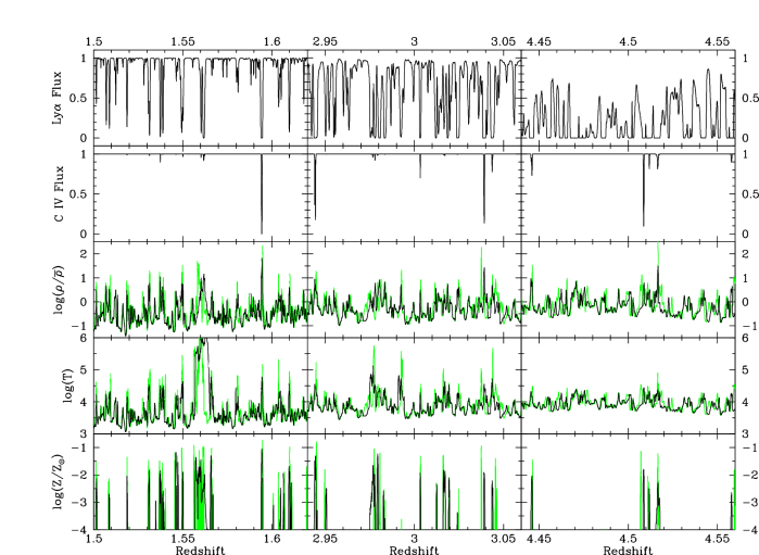
Figure 1: Example simulated spectra from the w16n256vzw simulation at three redshifts, $z\approx$ 1.5, 3.0, & 4.5, showing Ly$\alpha$ absorption, C iv absorption, and the underlying overdensity, temperature and metallicity distributions. Black lines show the properties with peculiar velocities and thermal broadening applied, while green lines show the underlying physical distribution.

Figure 1 demonstrates how Ly$\alpha$ flux, C iv flux, density, temperature, and metallicity appear at three different redshifts in one of our lines of sight. Some of the trends apparent in this model spectrum relate to the main conclusions of this paper. First, the evolution in C iv absorption is significantly less than that seen for Ly$\alpha$ due to the complicated interplay between enrichment, photoionization, and IGM heating in expanding large-scale structure. At higher redshifts, C iv absorption faithfully traces metal enrichment, but at lower redshifts this correlation becomes significantly weaker.

Except where noted, we will group individual Voigt-profile fit C iv absorbers (i.e. “components”) into “systems” if they lie within 100 $\;{\rm km}\,{\rm s}^{-1}$ of another. This is done in order to facilitate a more robust comparison among data of varying quality and to avoid systematics arising from different line fitting techniques. For example, in Figure 1, the C iv line at $z=1.594$ is a single component while the lines around $z=4.1$ form a multi-component system.

2.6 UV Background

We apply a spatially-uniform photoionizing background is taken from (2001) to the matter distribution, both during the simulation runs and during the spectral extraction. Unless otherwise noted, the background used is the one that is comprised of quasars and 10% of UV photons escaping from star-forming galaxies (referred to as QG), which turns on at $z\approx 9$. The slope of the QG background is softer than the (1996) quasar-only background short-wards of 1050 Å ($\alpha=-1.8$ vs. $\alpha=-1.55$).

The amplitude of the QG background can be constrained by approximately matching the Ly$\alpha$ flux decrement, $D_{Ly\alpha}$, to observed values over this redshift range. To do so, we divide the background amplitude by 1.6 at all redshifts to match the observed mean Ly$\alpha$ flux decrement, $D_{Ly\alpha}$. We do not do this during the simulation run, but only in post-processing as we extract the spectra, but as (1998) showed, because photoionization is subdominant in gas dynamics such a post facto correction yields virtually identical results as having done the entire run with the lower background.

In Figure 2 we compare the mean flux decrement in our spectra to measurements by (1993), (1997), and (2005), which have been corrected for metal line contamination. The (1993) functional fit and Rauch measurements are meant to measure the total $D_{Ly\alpha}$ as they apply corrections for their continuum fitting at high redshift, hence we do not continuum-fit our spectra for this comparison. Continuum fitting would have a non-trivial effect on $z\ga 3$ where the Ly$\alpha$ transmission almost never reaches 100% in our spectra. The difference declines at lower redshift; for instance, (1997) find that continuum fitting to the tops of Ly$\alpha$ peaks results in 5.7% flux loss at $z=3$ and 1.2% at $z=2$. The data points from (2005), which have been continuum fitted, show deviations in the highest redshift bins as expected. Their data agree within reason with our measurements, except at $z=3.0$ where they find a 22% lower $D_{Ly\alpha}$. Other than this measurement, we find that the HM01 ionizing background simply divided by 1.6 provides a good fit to the available data. The fact that we don’t need a redshift-dependent correction indicates that the HM01 background in conjunction with density growth in our assumed $\Lambda$CDM universe yields the correct evolution for $D_{Ly\alpha}$.

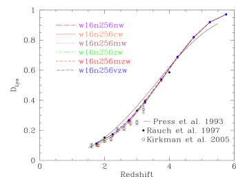
Figure 2: Lyman-alpha flux decrement ($D_{Ly\alpha}$) averaged over 30 lines of sight generated from each outflow simulation, using a HM01 background amplitude divided by 1.6 across all redshifts. This simple correction results in a simulated $D_{Ly\alpha}$ evolution generally in accord with observations. Our outflow models have little effect on $D_{Ly\alpha}$.

Interestingly, our outflow models have typically a negligible effect on the Ly$\alpha$ flux decrements, with the values mostly agreeing to 2% among the various simulations. This indicates that winds are not affecting the density and temperature structure over much of the Universe’s volume, or put another way, the filling factor of winds is fairly small (as we will show more quantitatively in §3.3). This is consistent with the results of (2002b) and (2006); the latter finding that the only quantitative effect of galactic winds on the Lyman-$\alpha$ forest is an increase in the the number of sub-Å saturated regions resulting from dense shells plowed up by the winds.

3 Global Physical Properties

3.1 Star Formation Rate Density

A major impetus for including superwind feedback is to suppress star formation and solve the overcooling problem. As SH03 showed, the constant wind model broadly matches the observed star formation history of the universe, the so-called Madau plot (, 1996). Here we examine Madau plots for our various wind models to ensure that they fall within the observed range as well.

Figure 3 shows the total star formation rate density as a function of redshift averaged over our three simulation volumes, for all our wind models. Data points shown are from a compilation by (2004). We include all star formation in each volume, without selecting out any particular galaxy population. In general, all our wind models roughly fall within the observed range down to their lowest redshift ($z=1.5$ or $z=2$), with possible discrepancies versus $z\ga 3$ data that are more poorly constrained. With no wind feedback, far too many stars are produced as found by SH03, while our various wind models suppress star formation at $z\sim 3$ by $\sim\times 3-5$ relative to no winds. Hence all our wind models broadly pass the Madau plot test.

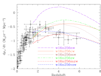
Figure 3: The total integrated star formation history compared to observations compiled by (2004). Wind models suppress star formation from the no-wind case (long-dashed) to bring then into broad agreement with data. The mass loading factor controls early star formation, while wind speeds become more important later on. Outflow models with large $\eta$ at early times suppress star formation, resulting in a peak in global star formation at later times.

More detailed examination reveals that there are some differences between wind models that yield insights into the impact of varying feedback parameters. For instance, in models where we have a variable $\eta$ (mzw,mw,vzw) that produces high mass loading factors at early times, we end up with a global star formation history that is peaked towards later epochs ($z_{\rm peak}\approx 2-4$) than in the constant $\eta=2$ cases (cw,zw) which show $z_{\rm peak}\approx 5$. This arises because the high early mass loading factors in small early galaxies keep gas puffy and warm, suppressing early star formation despite the fact that the wind velocities are low. As a case in point, note the vzw and mzw models show virtually identical star formation histories at high redshift despite having significantly different (mean) values of ${v_{\rm wind}}$, showing that it is indeed $\eta$ that primarily governs early star formation. The wind speed is not irrelevant, though, as that represents the only difference between vzw and mzw, and they show noticeable differences at later epochs. There, the universe becomes less dense, winds travel farther, and cooling rates are lower, so the wind speed ${v_{\rm wind}}$ increasingly governs the global star formation rate.

At face value, variable $\eta$ models appear to be in better agreement with observations that show $z_{\rm peak}\sim 2-3$, particularly the vzw model which shows a peak at $z\sim 2$. However, since we are not selecting galaxy populations in the simulation analogous to observed samples from which the data are calculated, such comparisons are at best preliminary. For now, we simply note that the feedback recipe can have significant impact on the global star formation history, including the peak of the star formation rate density in the Universe, and all wind models we consider here fall broadly within the allowed range.

3.2 Outflow Properties

As outflows represent the main new feature of our simulations, it is worth examining their properties in more detail. Here we highlight the differences between wind models in their typical speeds, mass loading factors, and energy deposition rates as a function of redshift. These provide useful background information for understanding the behavior of C iv absorption in our various outflows scenarios.

Figure 4 (upper left) shows the mean wind speed as a function of redshift for our various wind models. The zw and mzw models show similar wind speeds because they both employ equation 2, while the mw model shows lowered wind speeds primarily because it lacks the $2\sigma$ kick. The mean vzw wind speed is more in line with the mw model at $z\la 6$, but vzw produces a wider range of wind velocities due to its random assignment of $f_{L,\odot}$, and hence ends up being quite different than mw in many other ways. The boost from low-metallicity stars (not present in mw) is only important at very early times, because stars enrich themselves fairly quickly (, 2006), and once the metallicity exceeds around 1% of solar the boost becomes fairly small. The mean wind speed when we employ equation 2 becomes comparable to the constant wind case (horizontal line) at $z\sim 2$. It is worth noting that the wind speeds at $z\sim 3$ in all our models are comparable to the range of outflow velocities observed in Lyman break galaxies (, 2001).

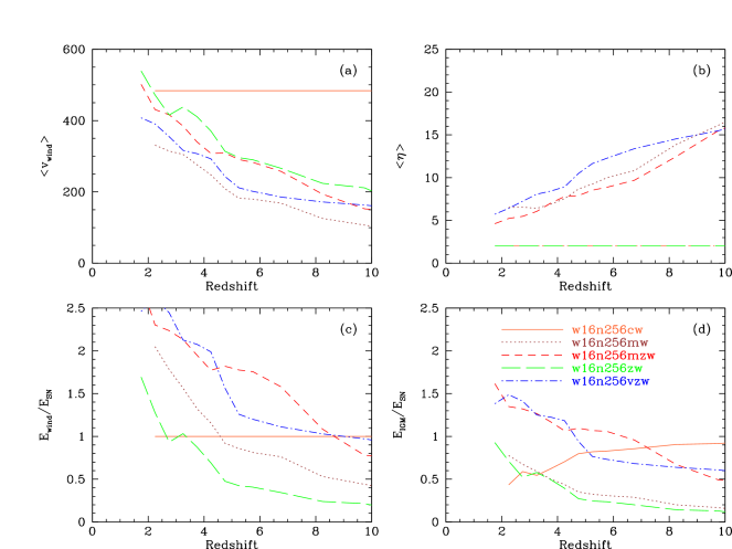
Figure 4: Wind property averages as a function of redshift for various outflow models. Panels (a) and (b) show the average wind velocity and mass loading factor, respectively. Panel (c) shows the energy inputted into the wind particles, and panel (d) shows the energy injected into the IGM, after we subtract the energy needed to leave the potential well of the galaxy. The energies are normalized by the energy injection from supernovae. The wind speeds and mass loading factors at $z\sim 2-3$ in momentum-driven wind models are in agreement with observations by (2001, 2006). The energy input can significantly exceed that from supernovae in our momentum-driven wind models, but this is physically plausible since radiation energy is the primary driver of momentum-driven winds.

The upper right panel of Figure 4 shows that allowing mass loading factor dependence according to equation 2 results in much more material being ejected from early galaxies. Of course, because the wind speeds are small and material is infalling gravitationally, the winds do not reach very far before being re-accreted. However, they do keep the gas somewhat hotter and more diffusely distributed around galaxies, so the high mass loading factors are effective at suppressing early star formation. Note that (2006) found that such suppression is necessary in order to match observed $z\sim 6$ galaxy luminosity functions. At low redshifts, (2006) estimated a required typical mass loading of around 4 in order to understand the trends observed in the galaxy mass-metallicity relation at $z\approx 2$; our momentum-driven winds broadly agree with this.

In the bottom two panels of Figure 4, we show the kinetic energy injected by the winds (left), and the amount of energy that reaches the IGM once subtracting off the energy required to leave the potential well and enter the IGM (right). We normalize these quantities to the average supernova energy for a Salpeter IMF, namely $4\times 10^{48}$ ergs per $M_{\odot}$ of star formation (the fiducial value used by SH03). The cw model was constructed by SH03 to return 100% of the supernova energy into kinetic feedback (although thermal feedback was included in addition), while the energy input from the momentum-driven wind models increases as galaxies grow. Eventually, the energy inputted by winds exceeds the supernova energy; this is physically possible because these winds are driven by UV radiation from massive stars over their entire lifetimes. An important feature of momentum-driven winds is that deeper potential wells in larger galaxies do not inhibit feedback of energy into the IGM, in accord with observations by (2005). The reverse is true for the cw model, where the energy injection into the IGM is quite high at high-$z$ and declines to lower redshift, which as we shall see leads to excessive heating of the IGM (see §3.3 and , 2005). Indeed, (2000) showed that metal enrichment via supernova-driven winds alone is energetically insufficient to enrich the IGM to the observed levels, and another unknown mechanism was required; momentum-driven winds provide such a mechanism.

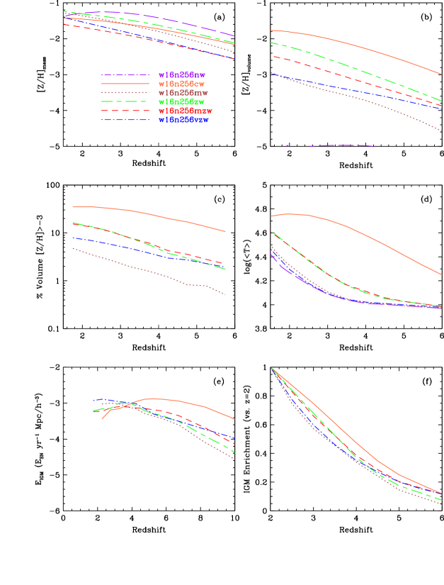
Figure 5: IGM properties averaged over the simulation box for various outflow models as a function of redshift. Panel (a) displays the global mass-weighted gas-phase metallicity, a quantity proportional to stellar mass except that the metals locked up in stars are not included. Panels (b) shows the volume-weighted metallicity, which is governed more by outflow speeds than by metal production, as the relative trends between models follow that seen in Figure 4a. Panel (c) shows the fractional volume of the simulation enriched to over [Z/H]$>-3$, which again is broadly governed by outflow speeds. Note that the no-wind cases is unable to enrich more than 0.1% of the volume at any epoch. Panel (d) shows the volume-weighted temperature, showing that constant winds dramatically enhances IGM temperature, while momentum-driven wind models heat the IGM substantially less. Panel (e) shows the amount of energy reaching the IGM in terms of supernova energy per year, per $h^{-1}{\rm Mpc}$; this is essentially a cumulative version of Figure 4d. Panel (f) shows the amount of metals in the diffuse IGM ($\rho/\bar{\rho}<100$) relative to the $z=2$ IGM metallicity; an increase of $\sim\times 10$ from $z=6\rightarrow 2$ is typical.

3.3 IGM Enrichment and Heating

Winds add metals and energy simultaneously to the intergalactic medium, and both quantities affect the characteristics of metal absorption in the diffuse IGM. In this section we examine how outflow parameters affect the evolution of metallicity and temperature in the IGM.

Figure 5, upper left, plots the mass-averaged metallicity in gas in our various runs. These curves track the cumulative amount of star formation in each run, with the slight difference that metals locked up in stars are not included in this plot. Consistent with expectations from Figure 3, the no-wind case has the largest amount of metal mass, while mzw and vzw have the smallest global metal production.

Comparing that plot to the volume-averaged metallicity in the upper right panel shows some interesting differences. Note that when quantifying IGM metallicity using absorption lines, it most directly traces the volume-averaged metallicity. In our outflow models, the amount of metals that enters into the IGM depends on a complicated interplay between the mass of metals (or stars) formed, the wind speeds, and the mass-loading factor. The large wind speeds in the constant wind case, together with relatively vigorous star formation, produce the most widely distributed metals, with a mean metallicity at $z\sim 3$ of $\approx 1$% solar. The difference between zw and mzw, which have similar wind speeds, arises because the low mass loading factor in zw yields more star formation and hence more metals. The lower wind speeds in mw and vzw produce relatively low volume-averaged metallicities. Canonical values inferred from C iv observations at $z\sim 3$ suggest [C/H]$\approx-2.5$ (e.g. , 1996, 1998), which is broadly consistent with all the wind models. We will engage in more careful comparisons to observations in §5.

The no-wind model does not distribute metals into the IGM hardly at all ([C/H]_volume never exceeds -5.0), leaving most of its volume pristine, and showing that dynamical stripping of enriched gas owing to interactions cannot enrich the diffuse IGM. Our results are in qualitative agreement with high-resolution Eulerian simulations by (1997) with no winds, having spatial resolution comparable to our runs but in much smaller volumes. They found a volume-averaged metallicity of $\approx 3\times 10^{-4}$ at $z=4$, which is an order of magnitude higher than what we find but is still much too low to enrich the diffuse IGM to the observed levels.

The two middle panels show the filling factor with metallicity greater than one-thousandth solar (left) and the volume-averaged temperature (right). The trends in these panels are related. In order to expel metals to large distances and fill volume, high wind speeds are required that results in high IGM temperatures. Hence the trends are similar among our wind models in the two plots: Constant winds produce high filling factors and large temperatures, zw and mzw are virtually identical, while the mw and vzw models fill less of the volume and hardly heat the IGM much above the primarily photoionization-established temperatures seen in the no-wind case. Interestingly, the spread of velocities in the vzw model both enrich the IGM while injecting relatively little energy, which as we will show turns out to be favored by observations.

The volume filling factor increases with time in all models because (1) metals have escaped their potential wells and are coasting away from their parent galaxies, and (2) galaxies are forming in less biased regions at later times. The volume filled in the cw model begins to asymptote as hierarchical buildup occurs and metals ejected by small galaxies falls back into larger halos. The volume will eventually asymptote for the other models, but at lower redshift since the smaller enriched volumes around galaxies will not overlap until later, and because the peak star formation is shifted to later epochs.

As a side note, (2000) demonstrated that at $z\sim 3$, the temperature of the IGM as traced by Ly$\alpha$ absorption line widths is $\approx 1.5-2\times 10^{4}$ K. This temperature is above that expected for pure photoionization (e.g. , 1996, or alternatively our no-wind case), which they interpret as arising from latent heat owing to He ii reionization. Our mzw and zw models broadly agree with the (2000) measurement, but in our case the excess heat is due to outflow energy deposition. Hence outflows can produce elevated temperatures without requiring He ii reionization (, 2003). We leave more detailed studies of Ly$\alpha$ line widths for future work.

The lower left panel of Figure 5 shows the energy injected into the IGM per year per $h^{-1}{\rm Mpc}^{3}$, in terms of amount of supernova energy produced. This energy injected is proportional to $\eta\times$SFR$\times v^{2}_{\rm IGM}$ where $v_{\rm IGM}$ is the velocity after leaving the potential well of the galaxy. The large amounts of early feedback energy in the cw model explains how its IGM becomes so hot by $z=6$. The momentum wind models peak in their energy output at $z=2-4$, with weaker winds peaking later. We will show later that this heat input results in significant variations in the global ionization fraction of C iv, which is a key ingredient in understanding C iv evolution.

The lower right panel shows the amount of metals in the IGM where $\rho/\bar{\rho}<100$ relative to that at $z=2$. This shows that in all models, the amount of IGM metals at $z=6$ is less than one-eighth of that at $z=2$. In other words, in all of our models the vast majority of metals are injected into the IGM during $z=6\rightarrow 2$, rather than at $z\ga 6$. Note that we do not include any “pre-enrichment” from exotic star formation at early times; our models are instead intended to test whether normal star formation in ordinary galaxies can enrich the IGM with outflow models included.

Overall, these results highlight the importance of the oft-overlooked connection between metal and energy input into the IGM. The mass-loading factor $\eta$ roughly governs the amount of total metal production at early times, while the outflow velocity ${v_{\rm wind}}$ mostly determines the physical extent to which the diffuse IGM ($\rho/\bar{\rho}<10$) is enriched and heated. As we shall see, the complicated interplay between metal production rate, wind speed, mass loading factor, and radiative cooling makes observations of IGM metallicity a highly sensitive probe of the physics of large-scale outflows.

4 Physical Properties of Metals and C iv Absorbers

4.1 Evolution of Metals in the IGM

Figure 6 shows density, temperature, metallicity, and C iv absorption at $z=$4.5, 3.0, and 1.5, in $15\times 15$ $h^{-1}{\rm Mpc}$ slices that are 100 $\;{\rm km}\,{\rm s}^{-1}$ wide, from the w16n256vzw model. We have deliberately centered the velocity slice on an overdense region (both in density and C iv absorption) to show the large variety of structures formed. This figure illustrates some of the trends that will be quantified in upcoming sections.

Figure 6: A 100 $\;{\rm km}\,{\rm s}^{-1}$ slice of the w16n256vzw simulation centered on a growing galaxy group at $z=$ 4.5, 3.0, and 1.5. In addition to the well-understood growth of large-scale structure (overdensity), the middle panels show that metal enrichment is tied with the early heating of the IGM, especially at high-$z$ before virialization dominates at low redshift. C iv absorption traces nearly all metals at high-$z$, and then declines to trace only the most overdense structures at low-$z$ as the overall ionization correction rises. Close inspection of the absorption structures indicates an evolution from smooth and diffuse to clumpy knots tracing the higher overdensities at low-$z$.

The growth of large-scale structure, dominated by gravitational instability, is evident in the gas density snapshots (top panels). Outflows increase the metal filling factor while growing the metallicity level in previously enriched regions. Bubbles of shocked gas grow around star forming systems and trace the filamentary structures that house galaxies. In the high-redshift snapshot, much of the heating is due to winds, as the hot bubbles trace precisely where the metals appear. Later, as a proto-group forms in the center of this region, the temperature also tracks the virialization of gas in the growing potential well. Interestingly, cold mode accretion (, 2005) is evident along the dense filaments feeding galaxies; hence despite the heat input, outflows do little to stop rapid accretion at high redshifts, because they tend to flow into lower density regions.

The C iv absorption is shown in front of a backlit screen to highlight the morphology of absorption, such as if our Universe was infinite and static (, 1826). In reality, quasars provide the backlight, and any quasar only probes a single pixel. At $z=4.5$, nearly all metals show C iv absorption when the ionization fractions are highest in the IGM. $\tau$(C iv)$\sim 0.05-0.10$ traces IGM gas with $\rho/\bar{\rho}=3-10$ and $\tau$(C iv)$>0.10$ traces $\rho/\bar{\rho}=10-30$ between $z=4.5-6.0$, a time when the vast majority of these overdensities remain unenriched by our prescribed winds. By $z=3.0$, metals have enriched the filaments, which show up as strong absorbers connecting the growing galaxy groups. By $z=1.5$, much of the diffuse IGM carbon is ionized to higher states, and C iv preferentially traces higher overdensity structure.

Figure 7 shows the mass and metal evolution in the diffuse IGM ($\rho/\bar{\rho}<100$, $T<30,000$ K) in the top panels, the warm-hot IGM (WHIM, $\rho/\bar{\rho}<100$, $T\geq 30,000$ K) in the middle, and the condensed IGM ($\rho/\bar{\rho}\geq 100$, includes stars) on the bottom for the cw, mzw, vzw, and nw models. The mass fraction in diffuse gas falls in all models from $z=6\rightarrow 2$, as mass transitions mostly to the WHIM phase resulting from both shock heating on large-scale structure and energy feedback. Not surprisingly, the WHIM fraction follows the mean temperature evolution in Figure 5. The no wind model provides a baseline for the amount of WHIM formed purely from growth of structure. At $z=2$, the cw model has a WHIM fraction of 50%, double the nw case, indicating half the WHIM results from feedback, and even more at higher redshift. The WHIM formed by energy feedback is moderate in the mzw case, and slight in the vzw model, thus leading to our conclusion that the fraction of WHIM formed by feedback depends most on wind speed. Meanwhile, the condensed phase understandably grows the fastest in the nw case, while the vzw model clearly distinguishes itself from other two feedback models shown here by producing more condensed matter resulting from low wind velocities unable to escape their parent haloes.

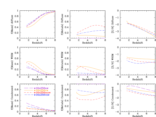
Figure 7: The fractional mass, fractional metals, and mass-weighted metallicity of the IGM (from left to right) subdivided into diffuse IGM ($\rho/\bar{\rho}<100$, $T<30,000$ K), warm-hot IGM (WHIM, $\rho/\bar{\rho}<100$, $T\geq 30,000$ K), and condensed IGM ($\rho/\bar{\rho}\geq 100$) (from top to bottom). The condensed component includes stellar mass and metals, although the [Z/H] measurement is just for the gas.

Both wind parameters, ${v_{\rm wind}}$ and $\eta$, have a significant effect on the fraction of metals in various phases, especially compared to the nw case where virtually no metals leave the condensed phase. The cw model has a significant amount of metals in the condensed phase due to its lower mass loading factor, but the metals that do escape into the IGM usually are shocked to WHIM temperatures. In momentum-driven winds (vzw and mzw), although $\eta$ is larger which suppresses star formation, the lower wind speeds allow more metals to return to the condensed phase, more so in the vzw case.

The mean gas metallicities (minus the stars in the condensed phase) are plotted in the right set of Figure 7. The condensed gas has a slowly-evolving metallicity of 5-20% solar in all wind models at these epochs at $z<4$. This enrichment level and evolution is similar to that seen for damped Ly$\alpha$ systems (, 2003), which are expected to arise in condensed gas. In contrast, diffuse gas shows a steadily increasing metallicity in all models, as star formation and winds combine to drive metals into the diffuse IGM. Interestingly, all wind models show similar diffuse phase metallicities and mass fractions, a result of the self-regulating nature of feedback (i.e. more feedback curtails star formation and metallicity enrichment). The WHIM at high redshift is primarily the result of feedback and is more enriched than the diffuse IGM. As virialization forms more WHIM at lower redshift, the WHIM metallicity becomes more similar to that of the diffuse IGM.

These figures illustrate that winds polluting the IGM also affect the temperature structure of the IGM, making C iv absorption an evolving tracer of metallicity. Next we quantify these trends from the perspective of C iv absorbers.

4.2 C iv Absorption in Phase Space

Currently the only observational probe we have of diffuse high-redshift IGM gas are one-dimensional quasar absorption line spectra skewering a complex matter distribution. In this section we present physical properties of the underlying gas for C iv absorption in our simulated spectra, in terms of the cosmic phase space (overdensity & temperature) of absorbing gas. We focus on the cw, mw, mzw, and vzw models as a representative range of wind scenarios: cw displays abundant early energy and metal injection, mw has comparatively little metals injection and almost no increased temperature compared to the no-wind case (see Figure 5), while mzw and vzw represent two intermediate cases that, as we shall see, are our favored models, with vzw being slightly preferred. Hence for illustrative plots we shall utilize the vzw model, with the understanding that the qualitative trends are similar in other models unless otherwise noted.

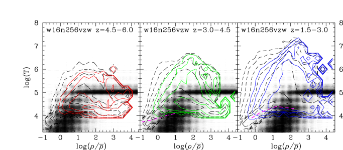
Figure 8: Solid (colored) contours show metal mass, while dashed contours show total mass plotted in $\rho-T$ phase space. Shading corresponds to the ionization fraction in C iv. These contours have 0.5 dex steps and are normalized across the three redshift bins. The shading goes from $0\rightarrow 40$% C iv ionization fraction, where the highest fraction occurs in collisionally ionized regions ($T\sim 10^{5}$ at $\rho/\bar{\rho}\ga 10$). The magenta dashed line in the lower two redshift panels is the $\rho-T$ relation used by (2003) to derive their metallicity-density-redshift relationship. Metals occupy a large region of phase space leading to a variety of ionization conditions that evolve with redshift.

Figure 8 shows the ionization fraction as a function of density and temperature, in three different redshift intervals for the w16n256vzw model. The ionization fraction shows two distinct regions: A horizontal band corresponding to collisional ionization around $10^{5}$ K, and a diagonal band at lower temperatures and densities corresponding to photoionization. Dashed contours overlaid on top of these shaded regions trace the total mass distribution from the vzw model. C iv absorption would be visible where these contours overlap the shaded regions, if metals are present. Metallicity (solid) contours that overlap shaded regions represent areas that are in fact traced by C iv for the vzw model.

One interesting result from this figure is that C iv is not an optimal tracer of photo-ionized IGM gas, particularly at lower redshifts. C v (40.3Å) would be a better tracer, but such an observation requires X-ray spectroscopy far beyond the current capabilities. Conversely, there is significant amounts of gas heated to around $10^{5}$ K in this and the other models, in which C iv should be prominent, even at high redshifts. The number of actual observed systems as a function of density is governed by an additional factor, namely the physical cross-section of the absorbing gas; this will be greater at lower densities, which is why weak C iv absorption is still more common despite having a relatively low C iv ionization fraction.

Comparing the solid and dashed contours also shows that in the diffuse IGM, which holds the majority of baryons and the vast majority of volume at these epochs, contains few metals. Hence the filling factor of metals is small (as seen in Figure 5), especially at high-$z$. The magenta dashed line in the two lower redshift bins is the density-temperature relationship used by S03 to derive their mass-metallicity relation, obtained by assuming that the metals occupy the diffuse IGM and can be described by a 1-dimensional $\rho-T$ relationship corresponding to the IGM equation of state. Their $\rho-T$ relation is flatter because they assume substantial latent heat from H i reionization at $z\sim 6$; we did not include this because latest results from the Wilkinson Microwave Anisotropy Probe show that the Universe was predominantly reionized out to $z\sim 10$ (, 2006), and our (2001) model assumes reionization at $z\approx 9$. The temperatures they use result in a global ionization correction that does not change much over their redshift range, leading to their conclusion that their lack of evolution in the C iv systems implies little redshift evolution in the true IGM metallicity. From this plot, it is clear that our self-consistent enrichment models predict C iv absorbers lying in a wider range of densities and temperature, and are not consistent with the assumption that C iv almost always arises in a photoionized phase. We quantify this in the next section.

Figure 9 compares the metal mass contours from the previous plot (shown as dashed contours) with the distribution of the actual C iv absorption (solid), in the $(\rho,T)$ plane, for the cw, mw, and vzw models (top, middle, and bottom panels, respectively). We obtain the C iv absorption density from the lines of sight in physical space, i.e. without peculiar velocities and thermal broadening that can significantly alter the relationship between absorption and physical properties. The two sets of contours illustrate the difference in phase space between the true metallicity and the metallicity traced by C iv.

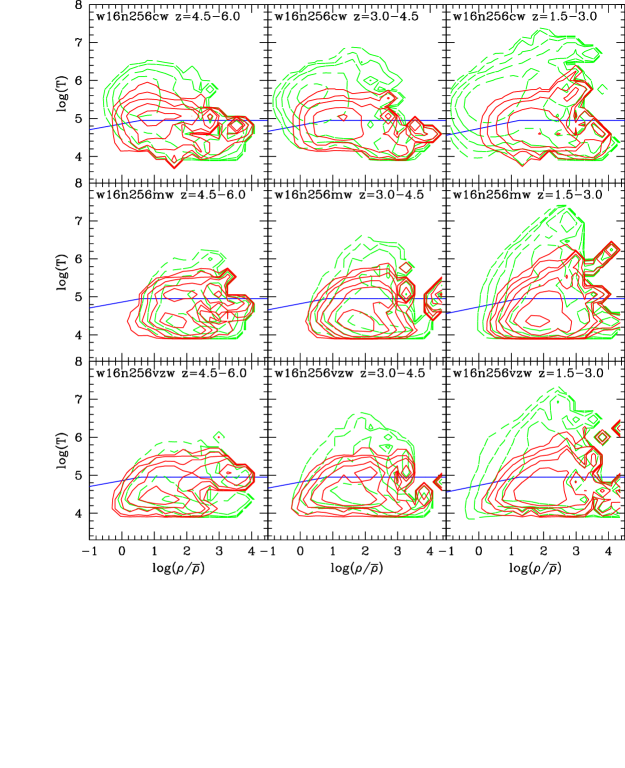
Figure 9: Dashed contours corresponding to metallicity mass (similar to those in Figure 8) and solid contours corresponding to the summed C iv optical depth (derived from lines of sight) in $\rho-T$ phase space for three different redshift from the w16n256cw, w16n256mw, and w16n256vzw models. The blue line divides regions dominated by collisional ionization (top) and photo-ionization (bottom). The cw model predominantly enriches the low density IGM while causing significant shock-heating, whereas the mw model enriches mostly higher overdensities and heating occurs mostly due to virialization at low redshift. The vzw model manages to enrich a variety of overdensities while causing little more shock heating than the mw model.

The three wind models shown tell very different stories about IGM metallicity, observed and actual. The constant wind model has high wind speeds and greater star formation at high redshift, resulting in earlier enrichment of lower overdensities and the shock-heating of the IGM. The C iv ionization fractions grow increasingly smaller at later times as the hot metals are ionized to higher states and cannot cool efficiently at such low densities. In contrast, the low wind speeds of the mw model copiously enrich high overdensities while minimizing shock-heating, and lead to a higher overall C iv ionization fraction, allowing C iv to more closely trace the metals. The intermediate vzw model with its variable outflow velocity has both higher wind speeds capable of injecting metals into the diffuse IGM and lower wind speeds replenishing metals in the galactic halo gas. The result is IGM enrichment at a wider range of densities than mw with less feedback heating than cw, which as we shall see is a better match to observations. All forms of feedback result in metals occupying a large range of temperatures by $z=3$ resulting in many metal lines being collisionally ionized, a prediction also made by (2002b) in their simulations with feedback.

Generally, at high redshifts C iv is a nice tracer of diffuse metals, but it misses the low-temperature high-density regime of the metal distribution (i.e. condensed phase metals) where much of the metals are residing. At $z<3$, C iv traces diffuse metals less well, because an increasing amount of metals arises in hot gas that is too highly collisionally ionized for C iv. It also fails to trace very diffuse gas that is too highly photoionized for C iv. Hence in what could be termed the “Age of C iv”, this ion between $z=3-4.5$ is able to trace metals over the largest range of overdensities corresponding to the largest variety of structures. As a side note, the relative invariance in C iv absorption across these redshifts can be seen by the similar areas covered by the C iv contours, despite the fact that the total metallicity (the area of the metallicity contour) is increasing with redshift; we will quantify this effect later.

In the low redshift bin, C iv traces typical overdensities of $\rho/\bar{\rho}\sim 100$ despite the peak in metallicity moving downwards to $\rho/\bar{\rho}\sim 30$. This indicates that C iv absorption, particularly strong absorption, is arising primarily in galactic halo gas. Unfortunately for our simulations, if the gas in these halos has a structure similar to our Milky Way with cold clumps (i.e. high-velocity clouds) and a complex multi-phase structure (, 1996, 2004), then we cannot hope to resolve the detailed density and temperature structure in our simulations. Indeed, observations by (2006) of quasar HS1700+6416 between $z=1.8\rightarrow 2.7$ suggest sub-kpc length scales for many of the strongest absorbers. However, lensed quasar image pairs do not show significant deviations until above a few hundred pc in C iv line profiles indicating highly ionized gas traces structure on at least kpc scales (, 2001). While these observations probe the IGM between $z=1.6\rightarrow 3.6$, smaller separations are probed at higher redshifts, so it is difficult to determine if the characteristic size of the absorber does in fact decrease at low redshift as our models predict.

Figure 9 further shows that C iv arises from both photo-ionized and collisionally ionized absorbers; we show a line above which collisional ionization dominates. Interestingly, the fraction of collisionally ionized C iv is highest at the earliest times despite a overall cooler IGM. The diffuse IGM densities are too high and the background is too low to ionize most metals to C iv, while at the same time the collisionally-ionized band intersects regions with metals heated almost entirely by early feedback. It is because of this that early observations of C iv absorption provide the greatest discrimination between feedback models, as we shall show more explicitly later on.

The fractions of C iv collisionally ionized between $z=5.5-6.0$ are 68% and 43% for the cw and vzw models respectively. These fractions fall precipitously to 29% and 15% by $z=4.0$, mainly because the photo-ionized C iv component rapidly increases due to the changing ionization conditions. The amount of collisionally ionized C iv never really drops, and grows rapidly below $z=2.5$ in the vzw model as metal-enriched gas collapses back into halos (especially overdensities $\rho/\bar{\rho}>300$) leading to a $\sim$50% collisionally ionized fraction at $z\sim 2$.

In summary, C iv absorption in cosmic phase space clearly demonstrates that there is no one simple C iv absorber type relevant to all redshifts and large-scale structures we are investigating. Instead, the photo-ionized and collisionally ionized absorption probe two different regions of the metal-enriched IGM that evolve independently over redshift. As the collisionally ionized component in particular is quite sensitive to the outflow model, C iv can in principle provide interesting constraints on galactic feedback, especially at early epochs.

4.3 Metallicity-Density Relationship

Since metals are generated in galaxies that lie at highly biased peaks of the early matter distribution (e.g. , 2006), it is expected that there will be a positive correlation between metallicity and local overdensity. Indeed, such a relation was determined based on C iv pixel optical depth statistics by S03. They inferred that the median metallicity followed the relation [C/H] = $-3.47+0.08\;(z-3)+0.65\;(\log(\rho/\bar{\rho})-0.5)$ between $z=1.8-4.1$, i.e. that IGM metallicity shows a moderate density gradient with little redshift evolution. Such a relationship provides a constraint on models of metal injection, though as we shall see this S03 relationship is sensitive to assumptions about the thermal state of the gas which are not supported in our more successful wind models.

The top panels of Figure 10 show the metallicity-density relationship for all our wind models at three redshifts. These are not log-linear relationships as have often been assumed in fits (e.g. SO3). Instead, the metallicity-density relations are generally fairly flat out to some moderate overdensity, and then drop increasingly rapidly to lower overdensities. Furthermore, metallicities are continually growing at all overdensities in all our simulations as outflows extend to lower overdensities and the condensed regions are constantly replenished with new metals from galactic superwinds.

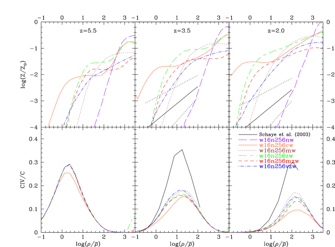
Figure 10: Top panels show the mean metallicity as a function of overdensity for all our wind models in three redshift bins. For comparison, the (2003) relation with its log-normal distribution is included at the two lower redshifts. All models show steady growth in metallicity at all overdensities as outflows reach lower overdensities while the metals are continuously replenished around galaxies. The bottom panels show the mean C iv/C ratio for all IGM gas independent of metallicity, demonstrating how the overall ionization fraction decreases and C iv preferentially traces more overdense gas. C iv absorption will be observed where the ionization ratio and the metallicity are both significant. The differences between the models result from the effect of feedback on the temperature structures of the IGM. The density-temperature relation assumed by S03 yields a steeper ionization fraction as a function of density (solid line), resulting in an inferred metallicity-density relation that is shallower than our simulations.

The cw model shows some different behaviors compared to the momentum-driven wind cases. The large early wind speeds in cw push metals so far out that the $<Z/Z_{\odot}>$ shows almost no gradient between $\rho/\bar{\rho}=1-10$, while various forms of the momentum wind models clearly show a gradient. For comparison, (2005) find a “metallicity trough” between $\rho/\bar{\rho}=0.1-1$ in their TIGER simulations, because their winds propagate from the most massive galaxies anisotropically, enriching the underdense IGM to higher metallicities than the filaments. The initial velocities in their model are 1469 $\;{\rm km}\,{\rm s}^{-1}$, which quickly slow down to a few hundred $\;{\rm km}\,{\rm s}^{-1}$ after accumulating material. Our cw model is probably most similar to theirs, but with lower outflow velocities that are not quite sufficient to produce a dramatic inversion in the metallicity-density relation.

The momentum-driven wind models have a stronger metallicity-density gradient, because smaller galaxies living at lower overdensities enrich smaller volumes with smaller velocities. The vzw model has the smoothest gradient resulting from the assumed spread in velocities enriching a variety of overdensities. The zw model, despite its significantly lower mass loading factor than mzw, enriches all overdensities more efficiently, because it has a higher overall star formation rate. Wind speed is the biggest determinant of metallicity in the diffuse IGM (especially at $\rho/\bar{\rho}<10$) while mass loading factor determines the metallicity of the condensed phases of the IGM ($\rho/\bar{\rho}>1000$); with larger values of $\eta$ removing more gas from galaxies, curtailing star formation, and decreasing enrichment. These difference emphasize the interplay of feedback, star formation, and energy deposition in the IGM.

Our metallicity-density relationship is generally higher than that inferred by S03 at most overdensities The primary reason for this discrepancy is the IGM temperature structure in our simulations. As we showed in §4, our simulated IGM is continually growing hotter at lower redshift making the C iv ionization fraction smaller where the metals are, and hence requiring higher true metallicities to match a given $\Omega$(C iv) absorption. To demonstrate this, the bottom panels of Figure 10 plot the overall C iv/C ratio (i.e. the inverse of the ionization correction) for all IGM gas independent of metallicity as a function of overdensity for the various models, along with that derived from the density-temperature relation assumed by S03 (the dashed line in Figure 8). C iv should be primarily observed at overdensities where both the metallicity and this ratio are large.

The S03 relation shows a much steeper ionization fraction growth with density in the mildly overdense regime than any of our simulations. This is because they assume pure photoionization, whereas our models have significant contributions from collisionally ionized C iv. This is even true of our no-wind model, owing purely to the growth of structure around galaxies. This explains why S03 obtains a shallower metallicity-density relation in this regime from C iv observations, while (as we will show in §5) we match similar data with our steeper metallicity-density gradient. Interestingly, (2006) suggested that a top-hat distribution of metals around galaxies is a better fit to the observed C iv auto-correlation function, as compared to the S03 fit. Our simulations produce a distribution that at least comes closer to this.

Figure 10 is also helpful in visualizing some of the trends described in §4.2. First, the C iv/C ratio peak shifts from overdensities of about 1 to over 100 from $z=5.5\rightarrow 2.0$, a startling increase due to the decreasing physical densities and (more weakly) the increasing ionizing background. The overdensities of the observed C iv do not shift as much because lower overdensities have less optical depth, plus the diffuse IGM has few or no metals at high-$z$ where the ratio is highest. Although the photo-ionized and collisionally ionized regions are distinct in $\rho-T$ phase space, the ratio merges into a single smooth peak when the temperature axis is collapsed (to visualize this look at the shading relative the the IGM dashed mass contours in Figure 8). Also, the overall decrease in the C iv/C ratio toward low-$z$ demonstrates the decline in the ability to use C iv as a tracer of metals.

The differences between outflow models isolate the effect of feedback on the temperature structure of the entire IGM. At $z=5.5$, feedback has not affected much the diffuse and underdense gas as can be seen by the similarity in the models; only the cw model is able to inject energy significantly to lower the ratio. During the Age of C iv at $z=3.5$, the ionization ratio is high at metal-rich overdensities high enough to create significant optical depth in all feedback models. The temperature structure causes the most divergence in the ratio by $z=2$ because of the transition to collisionally ionized C iv, especially in the cw model. Our models clearly contrast with the S03 linear density-temperature relationship, which intersects higher ionization fractions in the photo-ionized regime (see Figure 8), leading to their estimates of lower metallicity.

In short, C iv ionization conditions evolve with density and redshift, with an increasing contribution from collisionally-ionized absorbers at lower redshifts. Our metallicities at a given density are higher than inferred previously by S03 because the broad distribution of metals in the $\rho-T$ plane results in a higher overall C iv ionization correction.

4.4 Evolution of Median C iv Absorber in Phase Space

Figure 11 presents the evolution of absorbers in terms of the median phase space properties of C iv lines. We show three bins of column density (log($N$(C iv)) = 12-13 (weak), 13-14 (intermediate), 14-15 (strong)) over three different redshift ranges ($z=6\rightarrow 4.5$, $4.5\rightarrow 3$, $3\rightarrow 2$), for three of our wind models (cw, mw, vzw). The values are obtained by summing over parcels of gas in redshift space (i.e. including peculiar velocities and thermal broadening), and is thereby likely to underestimate the density and metallicity of the parcel(s) of gas contributing most to the absorption within a given line. This is more true at lower redshift as C iv absorbers become compressed in comoving space while the comoving pathlength per redshift increases. Nevertheless, these outflow models are clearly distinguished, allowing us to draw some simple conclusions about the physics of the absorbers.

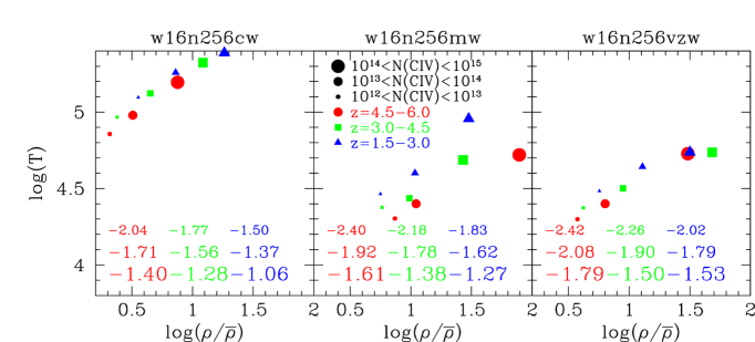
Figure 11: Median values of C iv absorbers subdivided into column density bins (point size) and redshift (color and shape) along with the median values of metallicity ([Z/H], written below with larger text for higher column density). Left, middle and right panels show the w16n256cw, w16n256mw, and w16n256vzw models. The medians plotted are derived from spectra that include peculiar velocities and thermal broadening. The cw model is dominated by collisionally-ionized absorbers at all redshifts, while mw is photo-ionization dominated. The vzw model probes the widest range of densities from weak to strong systems, showing its ability to enrich a wide range of environments, while still maintaining mostly photoionization-dominated temperatures.

In the cw model, the median absorber exists at a temperature that is dominated by collisional ionization ($\approx 10^{5}$ K), which as we shall show produces poor agreement with observations. The typical overdensity increases with time at all column densities, as diffuse gas becomes increasingly ionized to C v and beyond. In contrast, the mw model’s absorbers are almost always photo-ionized except at the strongest lines at high-$z$, and show relatively little evolution in overdensity over our redshift range, because the low wind speeds do not eject metals much outside the relatively dense regions that are well-traced by photo-ionized C iv. Meanwhile, the vzw model manages to shock heat more metals creating a larger collisionally ionized component, while concurrently allowing significant metal enrichment of denser halo gas by virtue of some outflow velocities being low. This creates a wider range of overdensities and temperatures traced by different column densities at any given redshift as compared with either the cw or mw models, with weak absorbers tracing $\rho/\bar{\rho}\approx 4-5$, and strong absorbers tracing $\rho/\bar{\rho}\approx 30-100$.

In brief, the behavior of C iv absorption in cosmic phase space shows noticeably different behavior for various wind models, suggesting that C iv observations can provide a sensitive probe of galactic outflows. In the next section, we demonstrate this explicitly by comparing our outflow models to observations.

5 Testing Outflow Models Against Observations

5.1 C iv Mass Density

So far we have seen that outflows can have a significant impact on the physical properties of the IGM. We now compare C iv absorption line properties from our various outflow models in order to determine which ones, if any, successfully reproduce available observations. We begin by examining the most global statistic that can be derived from C iv absorption, namely the total mass density in C iv absorbers, $\Omega$(C iv).

$\Omega$(C iv) provides a benchmark observational test for models of IGM enrichment. The observed lack of evolution of $\Omega$(C iv) from $z\approx 6\rightarrow 2$ has been cited as evidence for very early ($z\ga 6$) enrichment of the IGM (, 2001, 2002, 2005, 2005) from a putative generation of early massive stars and/or primeval galaxies. Such a scenario is attractive at face value because winds can easily escape the small potential wells of early galaxies. But it should be remembered that the metals must be expelled to densities approaching the cosmic mean in order not to have been gravitationally re-accreted onto galaxies by lower redshifts (e.g. , 2005). This means winds must not only escape galaxies, but must also overcome Hubble flow which is quite rapid at these early times, approaching 1000 km/s. A population of early galaxies that is energetically able to expel winds at $\sim 1000$ km/s may be difficult to reconcile with limits on pre-reionization massive star formation from the latest WMAP Thompson optical depth results (, 2006).

None of our models directly test this early IGM enrichment scenario. Instead, our outflow models attempt to reproduce the observed C iv evolution self-consistently from standard stellar populations combined with locally-calibrated outflow models. We find that our models are successful, thereby removing the need for widespread early IGM enrichment. We further find that observations non-trivially constrain our outflow models.

(2001) determined $\Omega$(C iv) by integrating the total column density of systems between $10^{12}\leq N$(C iv)$<10^{15}$ cm^-2 and dividing by the pathlength using

$$\Omega({\rm CIV})(z)={H_{0}m_{CIV}\over c\rho_{crit}}{\Sigma N_{tot}({\rm CIV},z)\over\Delta X(z)}$$ (5)

where

$$\Delta X(z)=\int{(1+z)^{2}dz\over\sqrt{\Omega_{M}(1+z)^{3}+\Omega_{\Lambda}}}.$$ (6)

These limits are chosen because larger column density systems are likely to arise from galactic halo gas, while the lower column densities suffer from observational incompleteness. When needed, we convert observations to our simulations’ $\Lambda$CDM cosmology ($\Omega_{M}=0.3$, $\Omega_{\Lambda}=0.7$). Measurements of $\Omega$(C iv) have highlighted some interesting trends that already provide a key test for our various feedback models.

Figure 12 shows the evolution of $\Omega$(C iv), as well as $\Omega$(C), calculated similarly to equation 5, except using the total metallicity along our simulated lines of sight. Observations of $\Omega$(C iv) by (2001), (2003), (2003), (2005), (2006), and (2006) are shown. We also show a measurement at $z\sim 0$ by (2003) for reference, although we will not compare to this data here.

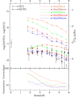
Figure 12: Evolution of $\Omega$(C iv) (closed circles) and $\Omega$(C) (open circles), the mass density in C iv and metals, respectively. Our five feedback models are compared to observations from (2001) (black circles), (2003) (small filled black squares), (2003) (open triangles), (2003) (open square), (2005) (large open dots), (2006) (large black squares), and (2006) (black triangle is a lower limit). All models show an increasing $\Omega$(C) over this redshift range, but most show a relatively constant $\Omega$(C iv). The ratio is shown as a “global ionization correction” in the bottom panel. The cw model is the most metal rich, and has increasingly large ionization corrections toward low redshift as the IGM is significantly heated and metals are pushed predominantly into low density regions. The weak momentum wind model (mw) produces little evolution in the ionization correction because it does not heat the IGM significantly, and hence is the only model that shows a rising $\Omega$(C iv) over the entire redshift range. The zw model overproduces $\Omega$(C iv) because it produces too many metals overall. The mzw and vzw models provide good fits to the observations, with the greatest discrimination between the two occurring at the highest redshifts. If further observations can confirm the lack of a downturn at $z>5,5$, another mechanism for early enrichment may be required.

The first striking result from this plot is that while the true IGM metallicity continually grows from $z=6\rightarrow 1.5$, most wind models show $\Omega$(C iv) to be relatively constant, and perhaps even decreasing at the lowest redshifts. This is especially true for our stronger wind models (cw, mzw, zw), indicating that outflows play a key role in governing C iv evolution. The key point is that in our models, $\Omega$(C iv) evolution is not a true indicator of metallicity evolution.

Two counteracting effects conspire to make $\Omega$(C iv) appear nearly constant. All feedback models grow IGM metallicity at a similar rate, but in the stronger wind models this is offset by a decreasing C iv ionization fraction owing mainly to an increasing IGM temperature from feedback energy. In the case where the feedback energy is minimal such as in the mw model, the globally-averaged ionization correction (shown in the bottom panel) remains more constant. Nevertheless, even this model’s ionization correction increases beyond $z=3$ as physical densities of the IGM decrease and the ionization background reaches its maximum strength. However, for feedback models that heat the IGM significantly (cw,zw,mzw), the ionization correction from C iv to [C/H] increases significantly with time, resulting a fairly flat $\Omega$(C iv) from $z=5\rightarrow 2$ despite nearly an order of magnitude increase in $\Omega$(C).

Intermediate wind-speed models, mzw and vzw, provide the best fit to observations of $\Omega$(C iv) over this redshift range. Recall that these are both momentum-driven wind models where $f_{L,\odot}=2$ and $f_{L,\odot}=1.05-2$, respectively. Indeed, the vzw model reproduces the most recent SuperPOD analysis by (2005, open circles) almost exactly, though without a more careful comparison to data this should not be taken too seriously. Interestingly, vzw and mzw provide good fits to $\Omega$(C iv) evolution for somewhat different reasons. In the mzw model substantial IGM enrichment is accompanied by significant heat input, so that ionization corrections evolves rapidly to maintain a roughly constant $\Omega$(C iv). In the vzw model, there is less IGM enrichment owing to lower wind velocities, but also less heat input. Indeed, mzw and vzw seem to bracket the allowed range of heat/energy input combinations: cw and zw produce too many metals in the IGM, while mw provides too little heat to obtain an ionization correction that grow sufficiently from $z=6\rightarrow 1.5$. Hence even from a relatively blunt tool such as $\Omega$(C iv), it is possible to place interesting constraints on outflow models.

To further constrain models using $\Omega$(C iv) requires probing to lower and higher redshifts. Lower redshift C iv observations should in principle be able to break this model degeneracy, but may be difficult to interpret because C iv traces increasingly denser regions that may be subject to multi-phase collapse, and the photoionizing background is more poorly constrained. Additionally, there is the observational challenge of C iv moving into the ultraviolet. Nevertheless, the determination of $\Omega$(C iv) in the local universe by (2003) would appear to favor a model with lower ionization corrections, since the IGM metallicity should level off because of the rapidly dropping global star formation rate at $z\la 1.5$. We leave comparisons to $z<1.5$ data for future work.

Conversely, moving to higher redshifts may provide more robust constraints. In particular, new observations by (2006) and (2006) at $z>5.5$ continue to show no apparent drop in $\Omega$(C iv) while our models predict a gradual decline. These measurements are dominated by a few strong systems (as these are the only ones detectable with current technology), so it is possible that may be associated with recent outflows that do not occupy a significant volume rather than indicative of widespread enrichment. Upcoming near infrared spectra of high-$z$ quasars discovered by the Sloan Digital Sky Survey should confirm just how widespread the C iv is, and whether our models require a further enrichment mechanism at high-$z$ or perhaps an increase in yields from the earliest stars. The lack of strong C iv observed above $z>5.90$ by (2006) along with the observation of a sudden increase in O i (2006) at $z>6$ may mean a sudden change in the ionization conditions of metals at this epoch corresponding to the last stages of reionization (2006) (R. Simcoe, private communication).

Finally, we examine a potential source of systematic uncertainty in comparing models to observations of $\Omega$(C iv), namely the effects of Helium reionization. The epoch and duration of He ii reionization is controversial, with some observations suggesting a rapid transition (, 1996, 2000, 2002a, 2004) at $z\sim 3$, while others favoring a more gradual evolution before $z=3$ (, 1998, 2003). Although the ionization potential of C iv is around 3.5 Ryd while He ii is optically thick above 4 Ryd, there may still be some residual effect on C iv absorption. To test this, we generate spectra using a soft QG ionizing background where we have reduced the photoionizing flux above 4 Ry by $\times 10$, and derive the resulting $\Omega$(C iv) evolution.

Figure 13 shows the results for the vzw case; the trends are similar for other outflow models. C iv traces less overdense material especially between $\rho/\bar{\rho}=1-10$, because of the lack of photons capable of ionizing C iv into C v; thus decreasing the overall C iv ionization correction. Hence if He ii reionization is a sudden process, there should a sudden decrease in $\Omega$(C iv) by a factor of around two at the epoch. Such a drop is not obvious in the data, although error bars are large and could conceivably hide it. At face value, it instead appears that He ii reionization is a gradual process, which could also somewhat affect the evolution of $\Omega$(C iv) possibly making this measurement even more constant over the redshift range. In fact, ((2006)) find evidence that the fluctuations in the He ii/H i ratio require a patchy background at energies $>4$ Ryd between $z=2-3$. We plan to examine the effects of this in more detail in the future.

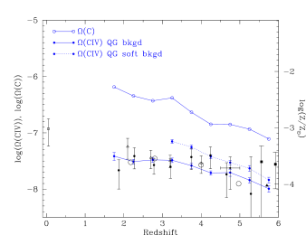
Figure 13: The comparison of the evolution of $\Omega$(C iv) with the standard (2001) ionization background (solid) and a softer ionization background where we have reduced the ionization at $>4$ Ryd by 90% to simulate pre-He ii reionization conditions above $z=3$ (dotted). The same data points described in Figure 12 are displayed. The soft background increases the observed C iv by as much as a factor of two. This difference favors a gradual He ii reionization, as a sudden transition would produce an observable drop in C iv.

To summarize, our models indicate that the invariance in $\Omega$(C iv) at $2\la z\la 5$ does not require the majority of IGM enrichment to occur at $z>5$. Our favored feedback simulations prefer an interpretation where metals injection follows global stellar mass production, but the accompanying energy injection conspires to make $\Omega$(C iv) roughly constant over the observed redshift range. We cannot rule out an early enrichment scenario that invokes a speculative early generation of stars to distribute metals in a manner that matches $\Omega$(C iv) data, but our self-consistent outflow models provide a more straightforward explanation.

5.2 C iv Line Parameters

5.2.1 C iv Column Density Distributions

While we showed that $\Omega$(C iv) can provide interesting constraints on outflow models, in fact there is more information contained in the statistical properties of C iv absorption systems from which $\Omega$(C iv) is derived. In this section we compare our models to observations of the column density distribution (CDD), which is the number of lines per unit redshift interval per log column density bin. The CDD is observed to fairly accurately follow a steep power law (, 2000, 2001). The slope, amplitude, and any deviations from this power law provide key diagnostics for testing models of IGM enrichment.

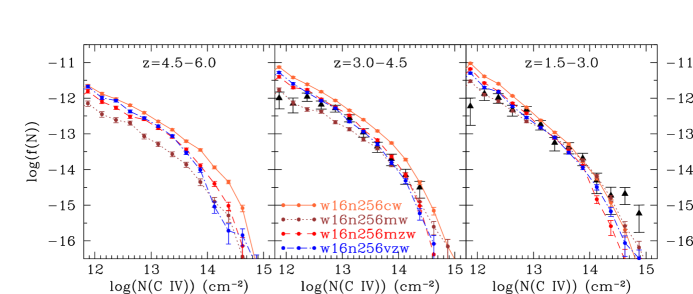
Figure 14: C iv Column density distributions for four of our outflow models in three redshift bins, compared to observations by BSR03 (black triangles). The cw model clearly overpredicts the CDD, while the mw predicts too few weak systems showing that its winds are too weak to enrich the low-density IGM. The mzw and vzw model provide promising fits to the data; the overprediction at weak column densities is likely a result of lower $S/N$ in the BSR03 data.

We use the AutoVP package (, 1997) to fit 30 simulated spectra per run generated continuously from $z=6\rightarrow 1.5$. For now we only consider the 1548 Å C iv component to avoid confusion; in real spectra, the sparseness of C iv absorption generally results in little ambiguity in line identification and characterization. This sparseness also provides a robust determination of the quasar continuum, so we do not continuum-fit our C iv spectra. (2000) demonstrated that AutoVP provided nearly identical fits to lines as the standard fitting package VPFIT (, 1987) for non-saturated lines (as is virtually always the case for C iv), and the quality of the fits in the figure appears good even in complex systems. One technical difference in fitting simulated spectra is that here we fit only the stronger component of the doublet, while observations generally require the presence of both doublet components to unambiguously identify C iv. Because of this, observations are more likely to miss weak lines. This difference is negligible when we integrate the total metal mass, but can become significant when we discuss the small-$N$(C iv) end of the CDD.

To compare our models with observations, we take line lists from 9 high-resolution spectra taken with HIRES published by (2003) (hereafter BSR03). The BSR03 data have typical signal-to-noise ratios of $S/N\sim 100$ and span $z=1.6\rightarrow 4.5$. We subdivide the BSR03 dataset into systems with $z>3$ and $z<3$, which covers a total of 9.19 and 7.73 in C iv redshift path length, respectively. We have also compared with line lists from 19 VLT/UVES spectra kindly provided to us by E. Scannapieco (, 2006), which covers a path length of 25.12 from $z=1.5-3.0$ with lower signal-to-noise than BSR03. However, the results are similar to BSR03, and the lower S/N and smaller redshift range motivates us to focus on the BSR03 data for clarity. In the future we hope to obtain the spectra themselves in order to do more careful comparisons including detailed noise characteristics and resolution effects (e.g. , 2001), but for now these data will suffice in order to ascertain the basic trends versus our various wind models.

Figure 14 plots CDDs for systems of C iv absorbers in three redshift bins, $z=1.5-3.0,3.0-4.5,4.5-6.0$. We will refer to these as the low, intermediate, and high redshift bins, respectively, throughout this paper (though we recognize that $z=1.5-3$ is not often regarded as “low” redshift). For simplicity we omit the zw and nw models from discussion, because the relevant trends are well-illustrated by the other four models (cw, mzw, vzw, and mw). Also shown are the BSR03 data (black triangles) in the relevant redshift ranges.

As can be seen, all the simulations generally produce a power law between $10^{12.5}\la N$(C iv)$\la 10^{14.5}$ whose shape is in agreement with observations. In fact, at early times the simulations show more of a deviation from a power law in the sense of fewer weak lines, because the enrichment has not spread yet to very low densities; such a trend is vaguely noticeable in the data as well. At the very lowest column densities the effects of incompleteness become significant. For concreteness, here are our completeness limits from simulated spectra with $S/N=100$: 75% for $10^{12.00}<N$(C iv)$<10^{12.25}$, 88% for $10^{12.25}<N$(C iv)$<10^{12.50}$, and 97% for $10^{12.50}<N$(C iv)$<10^{12.75}$. BSR03’s completeness limits are probably similar but somewhat lower given their requirement of identifying the weaker doublet line. As we are looking to understand general physical trends rather than engage in a detailed comparison versus observations, we do not attempt to mimic the data in any greater level of detail. We simply note that if a simulated CDD exceeds the data at the small $N$(C iv) end, one cannot draw conclusions from this without more carefully analyzing the incompleteness level in the data.

While qualitatively similar, these four wind models do show statistically significant differences, indeed quite large ones. The difference in CDD amplitude (and its evolution) tells basically the same story as the evolution of $\Omega$(C iv): cw produces too much C iv, while mw produces quite little, particularly early on. But the decomposition into column density bins provides additional information. For instance, the mw model does not enrich the low-density IGM much owing to its small wind speeds, and hence cannot produce enough weak lines at $z=3-4.5$ to agree with data. We note that the incompleteness in the observations is likely greater than that in the simulated spectra, so this effect works in the wrong direction to reconcile the mw model CDD. So even though mw looked promising at early times in the $\Omega$(C iv) comparison, it actually fails significantly when examining CDDs. In contrast, the mzw and vzw models provides very good agreement with observations, with the only discrepancies at $N$(C iv)$\la 10^{12.5}$ which may be explained by larger incompleteness in the observations.

Moving to the low redshift bin, model CDDs draw closer for two reasons. First, C iv traces denser gas where metals have been injected earlier on, and second because the metallicity in the denser regions starts to saturate, reaching an equilibrium between galaxies producing new metals and outflows driving those metals to lower densities. Again, there are still non-trivial differences, as cw still overproduces C iv absorption at all column densities, and mw still produces fewer weak lines. At face value the mw model seems to match the weak lines best, but recall that additional incompleteness in the data is quite significant here (particularly since the BSR03 observations with HIRES are less sensitive in the blue), so the turnover in the data at $N$(C iv)$<10^{13}$ may be at least partly artificial. There is a hint that all models produce too few of the very strongest systems with $N$(C iv)$>10^{14.5}$, which may be due to an increasing population of C iv absorbing gas in small, cold clumps that our simulations cannot resolve. For instance, (2006) derive small thicknesses ($<1$ kpc) and high overdensities ($\rho/\bar{\rho}>100$) for many of their strongest C iv components, which is below our spatial resolution limit.

Overall, the C iv CDD provides a sensitive test of the manner in which outflow models push metals into the IGM. Comparisons to observed C iv column density distributions favor the vzw and mzw models, which shows little redshift evolution at all but the smallest column densities, and whose total C iv absorption is close to that observed. More generally, it demonstrates that outflows must have wind speeds large enough to enrich the very diffuse IGM (giving rise to weak C iv absorption) at early times, but must not be so strong as to overproduce C iv absorption overall.

5.2.2 C iv Linewidths

While column density distributions probe the spatial distribution C iv in the IGM, line widths are more directly related to the temperature and dynamics of the absorbing gas. For H i, the line widths at $z\ga 2$ are dominated by Hubble flow broadening (e.g. , 1996), i.e. the cosmic expansion velocity spread across an unbound absorbing structure. This becomes less true at lower redshifts, where H i line widths obtain an increasing contribution from thermal broadening (, 2001), mainly because they arise in higher overdensity structures that do not have substantial Hubble flow across them (, 1999). In the case of C iv, even at high redshifts they arise in fairly overdense regions (see Figure 9), so we can expect that their line widths would have a significant contribution from thermal broadening.

Figure 15 shows histograms of $b$-parameters (i.e. Voigt profile line widths) of components with $10^{13}<N$(C iv)$<10^{14}$ cm^-2 in four of our outflow models for our three redshift bins, compared with BSR03 observations (filled circles in the lower two redshift bins). This column density range is optimal because observations both yield a statistically significant number of lines and generally approach 100% completeness. Arrows at the bottom of the plot show the median values.

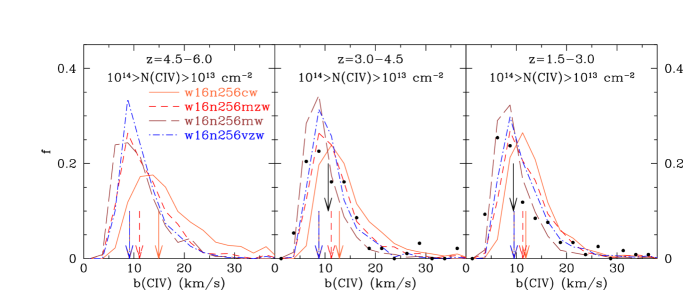
Figure 15: Line width ($b$-parameter) distributions for $10^{13}<N$(C iv)$<10^{14}$ cm^-2 systems for our various outflow simulations compared to observations by BSR03 (black dots). The arrows at the bottom show to the median values of the distribution for each model, and the top arrow is the median of the BSR03 data. The data agree with the mzw model at intermediate redshift, but suggest more compact, cooler C iv absorbers at low redshift such as those in the vzw or mw model.

The trends in this plot follow those in Figure 5, middle right panel (which showed the mean temperature evolution of the IGM). The cw model has significantly larger $b$-parameters owing to substantial shock heat input from outflows, and appears to be clearly discrepant when compared to observations. Indeed, the cw model actually has more lines ($\sim 66\%$) at $z>4.5$ that arise from collisional ionized C iv ($T\ga 10^{5}$ K, $b_{thermal}>11.8\;{\rm km}\,{\rm s}^{-1}$) than at $z<4.5$ where C iv is photoionized in cooler gas; this partly explains the $b_{med}$ evolution downward. Observations from BSR03 (solid points) suggest the mzw model is the best fit at intermediate redshift, while the vzw model better approximates the low-$z$ absorbers. The momentum-driven wind models (mw, mzw, vzw) are remarkable in that $b_{med}$ does not vary by more than 1 $\;{\rm km}\,{\rm s}^{-1}$ from $z=6\rightarrow 1.5$, especially considering that one of the main points of this paper is that C iv absorbers show significant physical evolution.

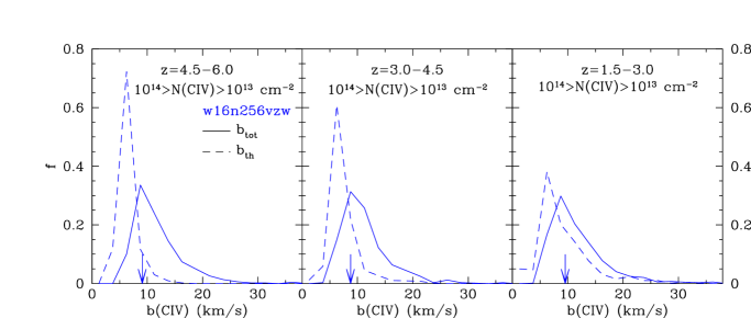
Figure 16: Histograms of total linewidth (solid lines) for the vzw model and thermal linewidth ($b_{th}$) derived from the temperature of the C iv absorbing gas (dashed lines). Thermal broadening comprises the majority of the total linewidth, especially at low redshift, showing that the $b$-parameter distribution can provide a sensitive test of feedback energy input into the IGM.

As an informative exercise, we subdivide the width of the vzw model line into a thermal component, $b_{th}$, that depends only on temperature, and a spatial component, $b_{sp}$, due to Hubble expansion across the physical extent of the absorber. We ignore turbulent broadening since the IGM at these overdensities is very quiescent (, 2005). Specifically, we assign $b_{tot}=\sqrt{b_{th}^{2}+b_{sp}^{2}}$, where $b_{th}=3.7\sqrt{T/10^{4}}$ for carbon, and $b_{sp}=H(z)\;w$(C iv) where $w$(C iv) is the spatial extent of the C iv. Figure 16 shows the total (solid) and thermal (dashed) $b$-parameter histograms for the vzw model, with $b_{th}$ calculated from the temperatures at the line centers. The thermal widths are the most significant component of the total line width, especially at low redshift, demonstrating (as expected) that at the moderate overdensities of C iv absorbers the Hubble broadening is sub-dominant. This implies that $b$-parameters can effectively trace the IGM temperature in C iv absorbing gas.

In summary, the line width distributions and the low-column density end of the CDD together put significant constraints on the wind speeds of early outflows: They must be strong enough to pollute the diffuse IGM at early times, but weak enough so as not to overheat the IGM. Some heating is accommodated, and in fact during the Age of C iv there is a hint that without wind heating, line widths are too narrow. More careful comparisons will be necessary to place more detailed constraints, but the fact that our locally-calibrated momentum-driven wind scenarios naturally fall within these relatively tight constraints represents a significant success for these models.

5.3 Pixel Optical Depth Statistics

The pixel optical depth (POD) method provides a powerful way to measure the metallicity in the diffuse IGM across a wide range of densities. The idea is to directly utilize optical depth information in the spectrum rather than fit lines, so that even weak absorption that would not yield a statistically significant line identification can be quantified. (1998) pioneered this approach, which was also used by (1998) to quantify O vi absorption in the crowded high-redshift Ly-$\alpha$ forest. More recently, (2005) and (2005) have expanded on POD analyses to precisely quantify C iv absorption in the IGM. In this section we compare POD analyses of simulated spectra with such observations.

In POD analyses, a histograms of optical depth ratios of two ions is constructed. This is done by identifying significant absorption in one ion, and examining the location in the spectrum where the other ion should be, and inferring the optical depth ratio of the latter to the former. In our case, we will consider C iv/H i and C iii/C iv ratios, in order to compare with data from (2005). Since C iii has a rest wavelength of 977Å, we must also correct for coincident absorption from H i Lyman series lines; we apply the method detailed by (2002) to do so. Specifically, the lowest order unsaturated Lyman-series line is used to determine the H i optical depth, which is then subtracted from all Lyman lines leaving the absorption component of any metal lines. Higher-order Ly$\alpha$ lines with their lower oscillator strengths allow one to probe much higher H i, up to $\tau$(H i)$>1000$ as opposed to $\tau$(H i)$\sim 3$ using Ly$\alpha$ alone. The POD method is surprisingly effective at extracting metal lines in the Lyman forest, although the effectiveness declines at $z>4$ due to the thick Ly$\alpha$ forest. While the full POD histograms are rich in information, for brevity here we focus on the median of the optical depth ratios as a function of H i or C iv optical depth.

We apply the POD method to the 30 lines-of-sight extracted from each simulation, where we include all 25 ions and continuum-fit the spectra blueward of Ly$\alpha$ as described in §2.6. We compare our results with POD statistics from (2005) for a sample of 6 quasars with $<z>\approx 3.1$.

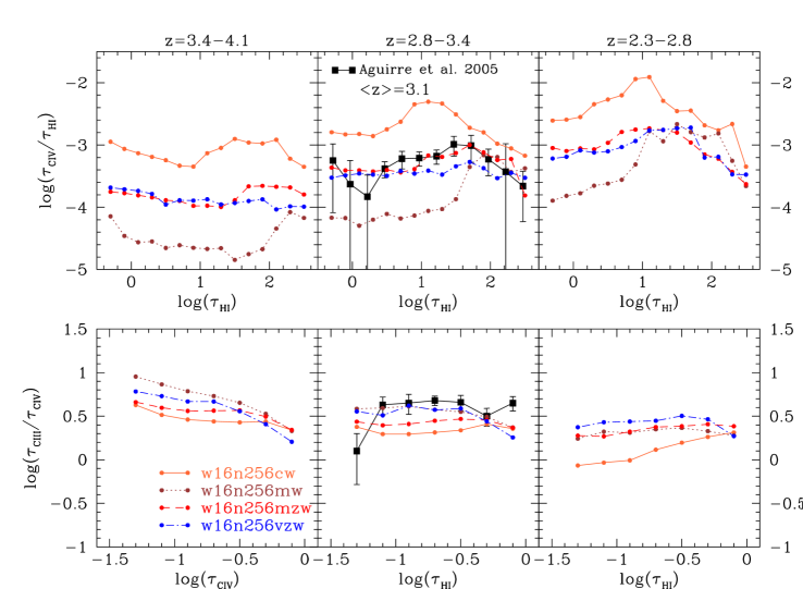
Figure 17: Median pixel optical depth ratios for our outflow models in three redshift bins, compared to observations by (2005) (solid lines). The mzw model provides the best fit to the observed C iv/H i ratio where H i is a proxy for overdensity, indicating that the metals are properly spatially distributed in this model. The vzw model does nearly as well, while the cw model injects far too many metals and the mw model is only able to enrich the most overdense regions. The vzw and mw models adequately fit the C iii/C iv ratio while the cw and mzw models underestimate this ratio due to excessive heating of the IGM. The mismatch at $\tau$(C iii)$\sim-0.1$ is likely a result of our simulated spectra having lower $S/N$ than the observations resulting in worse Lyman series subtraction at high optical depths in the C iii forest. The C iv/H i ratio grows toward lower redshift due to increasing metal enrichment, while the C iii/C iv decreases due to heating of the IGM and decreasing physical densities.

5.3.1 C iv/H i POD Statistics

Figure 17 (top panels) shows the median C iv/H i ratio as a function of H i optical depth for a variety of redshift ranges, for the cw, mw, mzw, and vzw models (left to right). This POD statistic shows even more dramatic differences between the various feedback models than the CDDs. For comparison, we plot the data from (2005) in the $z=2.8-3.4$ panels.

The overall trend is that the median POD ratio rises with time. This is primarily because the H i optical depth at a given overdensity is dropping more rapidly with time than the C iv optical depth because as the universe becomes less dense H i becomes more ionized, while C iv ionizing to C v is offset somewhat by C iii ionizing up to C iv. However, a secondary non-trivial effect is that the IGM is becoming increasingly enriched. While the median POD ratio is relatively flat with H i optical depth, the peak does shift to lower H i optical depth with time, owing to winds pushing metals further out into the IGM.

Comparing to observations, it is clear that the cw model overpredicts the median POD ratio at $z\approx 3.1$, consistent with over-enrichment of the IGM as has been seen from the $\Omega$(C iv) and CDD comparisons. What is new here is that the shape of the curve is also discrepant, in that the peak value is produced around $\log\tau$(H i)$\sim 1$, while observations prefer a peak at $\log\tau$(H i)$\sim 1.5$. This is indicating that metals are too widely distributed in the cw model, in addition to being overproduced.

The mw model represents the other extreme, where it fits only the high density regions ($\log\tau$(H i)$\ga 2$) but does not distribute the metals widely enough to match at $\log\tau$(H i)$\la 1.5$. Clearly, the winds are too weak in this model to enrich the diffuse IGM.

In contrast, the mzw does and excellent job fitting the full range of H i optical depths, indicating the winds are both producing the correct amount of C iv as well as distributing it correctly versus the underlying H i absorption. The vzw model is nearly as good, although it appears to produce slightly too little C iv absorption overall. Without doing a more careful comparison, we can only say that both these models are in reasonable agreement with observations.

(2005) applied the POD method on simulations including a 10 $h^{-1}{\rm Mpc}$, $2\times 216^{3}$ particle Gadget-2 simulation from SH03 (the Q4 simulation) with the cw feedback model, but without metal-line cooling. They added an ad hoc cooling method wherein SPH particles with cooling times less than Hubble times instantaneously reach $T\sim 10^{4}$ K; resulting in a C iv/H i ratio increasing by about $\sim\times 10$ with cooling. Using a test simulation, an 8 $h^{-1}{\rm Mpc}$ box vzw simulation with $2\times 128^{3}$ particles with and without metal-line cooling, we find the metal-line cooling increases C iv absorption only by between 60-90%, likely because in the denser regions the IGM is continuously reheated by feedback, while in the underdense regions the cooling time even with metals approaches the Hubble time. Hence the additional effects of metal line cooling cannot reconcile the cw model with observations.

5.3.2 C iii/C iv Statistics

The C iii/C iv POD relation is used by S03 to provide a constraint on the temperature of the absorbing C iv. This is a difficult measurement to obtain since C iii (977Å) is buried in the Ly$\beta$ forest, but their method applied identically to observations and simulations shows that the ratio can still be instructive. They conclude that the high ratios ($\tau$(C iii)$/\tau$(C iv)$>3$ at $z>3$) rule out large fractions of C iv-absorbing gas at $T>10^{5}$K where collisional ionization dominates and the ratio drops precipitously (refer to their Figure 7 to see how this ratio depends on density and temperature using the QG background). (2005) find that their Gadget-2 simulation remained much too hot to reproduce the observed ratio, and ratios were 0.65 dex too low even when including metal cooling, only a modest improvement.

We find that our cw model indeed produces too low a median POD ratio. This indicates that the IGM is too hot in this model compared with observations, as we also saw in the $b$-parameter comparison. In contrast, our momentum-wind models fare considerably better. The mzw model still appears to heat the IGM too much, but the vzw and mw models (with relatively low wind speeds that do not add much heat to the IGM) fare quite well.

S03 points out that the observed C iii/C iv ratios are inconsistent with the absorbing gas being at $T\ga 10^{5}$K. However, even the vzw and mw models have a substantial fraction of their C iv-absorbing gas collisionally ionized, about 30% at $z\sim 3$. Despite this, these models match the POD ratios quite well, showing that some collisionally-ionized C iv is still accommodated by observations.

S03 further observes a gradual decline in $\tau$(C iii)$/\tau$(C iv) with time. All wind models produce a gradual decline qualitatively consistent with these data. In photo-ionized gas this decline is mainly driven by Hubble expansion increasing the IGM ionization level, and secondarily by the increasing temperature of the IGM.

In summary, pixel optical depth techniques provide a complementary technique to Voigt profile fitting for examining IGM C iv absorption. The overall results from both of these techniques support the same basic conclusions: Our cw model overproduces metals, distributes them too widely, and makes the IGM too hot, while the mw model underproduces metals, does not distribute them widely enough, and keeps the IGM (possibly) too cool. In between lie the mzw and vzw models that seem to span the allowed range of metal and energy input. More generally, these observations already provide a non-trivial bracketing of the allowed energy and metal input into the IGM as a function of redshift. More careful comparisons with observations, particularly pushing to higher and lower redshifts, should allow us to provide strong constraints on the properties of galactic outflows across cosmic time.

6 Numerical Resolution

Numerical simulations by necessity have a finite dynamic range, and even advanced ones such as ours cannot fully resolve the relevant scales from star formation to the Hubble volume. Hence we must ensure that our results are not sensitive to issues of numerical resolution. For this purpose we have run with 8, 16 and 32 $h^{-1}{\rm Mpc}$ box lengths, as described in §2, which span a factor of 4 in spatial resolution and a factor of 64 in mass resolution . The results presented so far have been derived from the $16h^{-1}{\rm Mpc}$ volumes for each outflow model, because as we will show in this section, their results show good convergence relative to the higher-resolution $8h^{-1}{\rm Mpc}$ runs (at least for the momentum-driven wind models), but the $32h^{-1}{\rm Mpc}$ runs do not show good convergence. We present simple arguments that explain this behavior in terms of the Jeans length in the moderately-overdense IGM giving rise to C iv absorption. Finally, we show that the constant wind model shows poor convergence at all resolutions. We focus on the convergence properties of the observable quantities that we have compared to in previous sections.

In Figure 18 we show $\Omega$(C iv) and $\Omega$(C) (or more accurately the carbon in the IGM) for the cw (top) and vzw (bottom) models. The cw model shows poor convergence, with more metals and C iv absorption being produced in higher resolution simulations. This is in stark contrast with the global star formation rate in these models, which shows excellent convergence at late times as demonstrated by SH03 (higher-resolution simulations do resolve earlier star formation). In the cw model, all galaxies roughly enrich the same volume independent of galaxy mass since they eject winds at the same speed. Hence higher resolution simulations that resolve star formation in smaller halos at earlier times distribute metals much more widely. To obtain a convergent IGM enrichment in a constant wind model requires resolving every galaxy that has ever driven a wind, which is exceptionally challenging computationally. Since the disagreement with observations is even greater in higher resolution runs, this model is unlikely to be successful in explaining IGM enrichment.

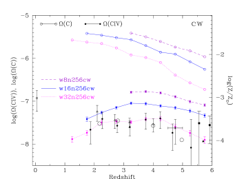
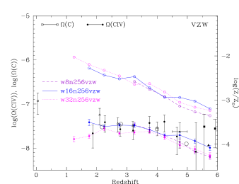
Figure 18: The numerical resolution dependence of $\Omega$(C) (as measured along our lines of sight) and $\Omega$(C iv) in the cw and vzw models in the 8, 16, and 32 $h^{-1}{\rm Mpc}$ boxes with $256^{3}$ gas and dark particles. The same data points described in Figure 12 are displayed. $\Omega$(C) and $\Omega$(C iv) converge quite well in momentum-driven wind models, unlike for the constant wind case. The $\Omega$(C iv) measurement suggests slightly larger ionization corrections at lower redshift in larger boxes.

The vzw model, on the other hand, shows much better resolution convergence over most of the redshift range in both $\Omega$(C iv) and $\Omega$(C), with a minor exception at $z\ga 5$ where the stochastic nature of biased early star formation may be producing differences between the realizations.

The impact of a finite volume is also seen in the vzw model at $z\la 3$. Here, the $32h^{-1}{\rm Mpc}$ volume produces a larger global C iv ionization correction, owing to larger and hotter structure being formed in the larger volume. The differences are small, but illustrate that large volumes are needed as well as high resolution in order to properly model the IGM. Hence it is desirable to use the largest possible volume that is resolution-converged.

Despite these minor issues, our overall conclusions should be robust as long as the simulations are capable of accurately resolving the properties of C iv absorbers. As Figure 19 shows, this is a good assumption for the CDD, with the 8 and $16h^{-1}{\rm Mpc}$ vzw volumes showing good convergence over most of the redshift range. The other momentum-driven winds follow similar trends, while cw is not converged (as with $\Omega$(C iv); not shown). The deviations in the vzw case are primarily associated with the $32h^{-1}{\rm Mpc}$ volume. It underestimates weak absorbers at high-$z$ because it cannot fully resolve all metal production, and it underestimates strong absorbers at low-$z$ because strong C iv systems arise in small galactic halos that it cannot resolve. Hence our 16 $h^{-1}{\rm Mpc}$ volume is optimal. Unfortunately, we cannot directly determine if our 16 $h^{-1}{\rm Mpc}$ volume is robust at $z<3$, since we have only evolved our 8 $h^{-1}{\rm Mpc}$ volume to $z=3$ due to CPU time considerations. Some effects of multi-phase collapse in high density regions may therefore persist in this volume, which may explain the deficit present in all models compared to data at the largest column densities.

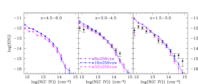
Figure 19: Column density distributions of C iv for the w8n256vzw, w16n256vzw, and w32n256vzw simulations, compared to the BSR03 points (black triangles). The 8 and 16 $h^{-1}{\rm Mpc}$ simulations appear resolution converged, while the 32 $h^{-1}{\rm Mpc}$ box underestimates weak absorbers at high-$z$ and possibly stronger absorbers at low-$z$.

The linewidths provide an even more stringent test of resolution, because they are keenly sensitive to small fluctuations in diffuse gas. Figure 20 shows the $b$-parameter distribution for the vzw model in three redshift intervals. While the 8 and $16h^{-1}{\rm Mpc}$ agree very well, the w32n256vzw model clearly shows wider $b$-parameters at all redshifts. If we split the width of the lines up into their thermal and spatial component as we did in §5.2.2, we find that the increase is mostly in $b_{sp}$. At $z>4.5$, we find $w$(C iv)$=12.7$, 11.5, and 16.5 kpc for the 8, 16, and 32 $h^{-1}{\rm Mpc}$ boxes respectively. Hence the line widths, as with the CDDs, are well converged up to $16h^{-1}{\rm Mpc}$ but falter at lower resolution.

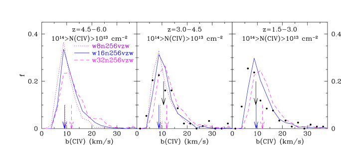
Figure 20: The $b$-parameters distributions in our three volumes for the vzw model. This demonstrates the w8n256vzw and w16n256vzw absorbers are resolution-converged and fit the observations by BSR03, while the w32n256vzw absorbers are too wide. Using a Jeans length argument (see text), we show that the 32 $h^{-1}{\rm Mpc}$ often has too poor resolution to properly resolve diffuse C iv absorbers.

Can we understand why the 16 $h^{-1}{\rm Mpc}$ volumes are converged but 32 $h^{-1}{\rm Mpc}$ ones are not? To do so, we estimate the minimum spatial resolution needed to properly model IGM fluctuations at any given density. We begin with the minimum SPH resolution, which is approximately $0.5~{}l_{box}/n_{part}\times(\rho/\bar{\rho})^{-1/3}$, or $0.5~{}\bar{d}_{mis}(\rho/\bar{\rho})^{-1/3}$ where $\bar{d}_{mis}$ is the mean interparticle spacing (i.e. a single resolution element generally requires two SPH particles in any given direction). The physical minimum optically-thin absorber size depends on the Jeans length, the limit below which the thermal kinetic energy prevents the IGM from collapsing. The Jeans length is $r_{j}=975~{}\sqrt{T_{4}/[(\rho/\bar{\rho})(1+z)^{3}]}$ kpc at a given density $\rho$, where $T_{4}=T/10^{4}$. Equating the minimum SPH resolution to $r_{j}$, we derive the following expression for the maximum interparticle spacing allowable in a simulation to resolve an absorber,

$$d_{res}=170~{}(\rho/\bar{\rho})^{-1/6}(4/(1+z))^{-3/2}\sqrt{T_{4}}~{}h^{-1}{\rm kpc}.$$ (7)

Because of the inverse density dependence in $d_{res}$, SPH simulations actually tend to resolve the low-density IGM fluctuations slightly better than the high-density ones, at a given temperature. However, particularly at high redshifts, low-density fluctuations tend to be colder (see Figure 11), making them the dominant resolution constraint. The typical value of 170 $h^{-1}{\rm kpc}$ above is uncomfortably close to our 32 $h^{-1}{\rm Mpc}$ volume’s $\bar{d}_{mis}=125h^{-1}{\rm kpc}$, hence this volume is starting to fail to resolve some absorbers, resulting in poor convergence.

At low-$z$, (2006) observed strong metal-line absorbers to have $T\sim 10^{4}$ K and $\rho/\bar{\rho}\sim 100$ between $z=2.7\rightarrow 1.8$. These are similar to the physical parameters of our strongest C iv systems at these redshifts. At $z=2$, we obtain $\bar{d}_{res}=51h^{-1}{\rm kpc}$ for these parameters, which would not quite be resolved even in our 16 $h^{-1}{\rm Mpc}$ runs ($\bar{d}_{mis}=63h^{-1}{\rm kpc}$). Hence the deficit in strong systems in our models may be due to lack of resolution.

To summarize, the resolution convergence for the vzw model is quite good up to our $16h^{-1}{\rm Mpc}$ volume, which is precisely why we chose to quote predictions for this volume throughout the paper. Our $32h^{-1}{\rm Mpc}$ shows poorer convergence, but it also suggests that at lower redshifts ($z\la 3$) the small $16h^{-1}{\rm Mpc}$ volume may slightly impact strong absorber statistics. We have checked that our results for the vzw case are generally applicable to all the momentum-driven wind models. In contrast, the cw model shows poor resolution convergence, and the disagreements with observations are significantly exacerbated as one moves to higher resolution.

7 Conclusions

We have explored various models of galactic outflows incorporated into cosmological hydrodynamic simulations of structure formation, and compared them with observations of IGM enrichment at $z\ga 1.5$. With no outflows, we show (in agreement with previous studies, e.g. , 2001) that a smattering of metals are distributed out to moderate overdensities through dynamical interactions, but cannot come close to enriching the diffuse IGM to observed values. Hence high-velocity outflows are required to enrich the IGM to observed values. In order to allow flexibility and perform controlled tests of various scenarios, we implement these outflows “by hand”, tying the wind velocities ($v_{w}$) and mass loading factors ($\eta$) to galaxy properties through various parameterizations.

In this paper we show tests of five outflow models. Most of these models, and all successful ones, are based on momentum-driven wind scenarios that are favored by observations of local starburst galaxies. We consider a constant-wind (cw) model that produces strong, early outflows; a weak momentum-wind model (mw) that yields little IGM heating; an “observed” wind model (zw) obtained by taking the observed scalings of local outflows at face value (not a momentum-driven scenario); a strong momentum-wind model (mzw) calibrated by local starburst observations of (2005); and a variable momentum wind model (vzw), where we have included a spread in wind speeds in accord with observations of (2005). Our models are chosen to span an interesting range in outflow strengths, while broadly reproducing the global star formation rate density evolution down to $z=1.5$.

Our first main result is that the outflow models favored by local starburst observations, when applied to galaxies forming hierarchically across cosmic time, are able to reproduce a wide range of C iv absorption line observations during the epoch of peak cosmic star formation ($z\sim 1.5-5.5$). We further demonstrate that this agreement is non-trivial, requiring particular levels of metal and energy input into the IGM as a function of time. In particular, winds should have high enough speeds to enrich the diffuse IGM at early times, but low enough speeds not to overheat the IGM. Winds should also have mass loading factors high enough to suppress early star formation, but low enough to produce enough early metals. Generically, momentum-driven wind models produce the desired scalings, because they heavily suppress early star formation but are able to distribute many of the metals formed into the IGM due to the high early mass loading factors in small galaxies. Yet, their low wind speeds from small galaxies do not overheat the IGM. It is therefore quite remarkable and non-trivial that our stronger momentum-driven wind scenarios (mzw and vzw), based on physical models calibrated by local observations of outflows, naturally reproduce a wide variety of observations.

Our second key result is that the lack of evolution observed in the properties of C iv absorption such as the global mass density in C iv systems ($\Omega$(C iv) from $z\sim 5.5\rightarrow 1.5$ is not necessarily indicative of a lack of continual enrichment, as has been argued previously (e.g. , 2001, 2002). In all our models, most of the metals are ejected into the IGM during the heydey of star formation at $z\la 6$, but our successful models also inject sufficient heat into the IGM to generate a drop in the C iv ionization fraction that roughly balances the increase in metallicity. The success of the mzw and vzw models in matching $\Omega$(C iv) evolution renders unnecessary a putative population of early star formation that enriches a large fraction of the IGM at $z\ga 6$.

Comparing various models to $\Omega$(C iv) data showed that C iv is overproduced in the cw and zw models, primarily because early star formation is insufficiently suppressed and copious metals are produced. While the large heat input from the cw model partially counteracts metal overproduction by lowering the C iv ionization fraction, it is insufficient to bring this model into agreement with data. Note that a comparison to observed $z\sim 6$ galaxy luminosity functions by (2006) also indicated that star formation is not suppressed sufficiently early on in the cw model. One could envision lowering the wind speed in the cw model to reduce the heat input and lower $\Omega$(C iv), but this would exacerbate the overcooling problem at high redshifts. The highest-$z$ observations of $\Omega$(C iv) tend to favor models that suppress early star formation, which occurs naturally in the momentum-wind driven scenarios (mzw, vzw) owing to high mass loading factors in small galaxies.

The column density distributions of C iv absorbers present a test of the spatial distribution of metals. Models with overly weak winds such as mw cannot pollute the low overdensity ($\rho/\bar{\rho}\sim$ few) IGM to reproduce the population of weak absorbers seen at $z\sim 3-4$. Once winds are strong enough (vzw, mzw, even cw and zw), the shape and (lack of) evolution of the CDD is roughly as observed.

Observations of the C iv linewidth ($b$-parameter) distribution shows little evolution, which again is generally reproduced in all our models. The linewidths provide constraints on the temperature of absorbing gas, which seem to accommodate some but not too much feedback energy input, as provided by the vzw, mzw, and mw models.

Pixel optical depth (POD) ratios provide a different way of characterizing C iv absorption, yet yield broadly similar conclusions. The C iv/H i POD ratio tests the amount and spatial distribution of the metals, because H i absorption is correlated with underlying gas density. Comparisons with our models show that cw distributes metals too widely, mw not widely enough, and mzw and vzw lying in the intermediate range that agrees with data. The C iii/C iv POD ratio is a sensitive measure of temperature, and shows that the cw and possibly even mzw heat the IGM too much, while the vzw and mw models match well.

In short, vzw and to a slightly lesser extent mzw are the only models that match all observations of C iv absorption we have considered, while reproducing a promising match to the global observed star formation history. These observations provide sensitive tests of the metallicity and temperature structure of the IGM, making the agreement of these models an impressive achievement. The fact that these models are consistent with local observations of outflows provides an interesting connection between starbursts-driven outflows at all epochs.

Our simulations also provide insights into the physical effects of outflows on the IGM. Both the vzw and mzw models show relatively low volume filling factor of $Z>10^{-3}Z_{\odot}$ gas, increasing from $\sim 2\rightarrow 10$% from $z=6\rightarrow 2$. Hence widespread enrichment of the IGM is not required to match observations, and in fact is disfavored as models that distribute metals more widely tend to overproduce C iv absorption. These results broadly agree with measurements of the quiescence of the IGM at high redshift that suggest outflows cannot have impacted a significant volume (, 2005). The metallicity-overdensity relation in the IGM is not a power-law as is sometimes assumed, and instead shows relatively flat enrichment at high overdensities, dropping off steeply at lower overdensities. An interesting prediction of our models is that a significant fraction of C iv lines are collisionally ionized. However, this does not violate temperature constraints on the IGM as seen from $b$-parameter distributions or C iii/C iv POD ratios. The median C iv absorber traces higher overdensity and hotter gas at lower redshifts, and the optical depth is only weakly correlated with underlying gas density, unlike the tight relationship inferred for Ly$\alpha$ absorbers (e.g. , 1999). This primarily owes to the large range of ionization fractions in C iv systems, from cooler photoionized absorbers to collisionally ionized systems reaching $T\sim 3\times 10^{5}$K. The idea that C iv absorption arises almost exclusively in diffuse, photoionized gas following a tight density-temperature relation similar to H i absorbers is not favored by our models.

While we present five wind models in this paper, we have actually simulated over a dozen wind models, and decided to focus on these five because they are physically and/or observationally motivated, and best illustrate the relationship between outflow properties and IGM enrichment. Nevertheless, the range of outflow models investigated in this work is far from exhaustive, as one could envision more complex recipes that might still be consistent with observations. Hence our favored models should be regarded as plausible, but not uniquely successful.

Further uncertainties in the exact model that best describes galactic outflows comes from a range of systematic uncertainties we have not extensively considered in this work. One uncertainty is the impact of Helium reionization (investigated briefly in §5.1), which can impact the comparison of C iv absorption at early epochs. Unfortunately including this effect requires fairly precise knowledge of the topology and epoch of Helium reionization, which is poorly constrained at present. A second uncertainty is that our simulations were run with a cosmology that is slightly different than that now favored by the 3rd-year WMAP release. In particular, the new values of $\sigma_{8}$ (now 0.75 as opposed to 0.9 as we used) and $\Omega_{m}$ (0.24 vs. 0.30) will significantly lower the halo collapse fraction at high redshift (, 2006). This means that the mass loading factors will need to be reduced relative to equation 3 to match observations of high-redshift star formation rates. The net effect should be small: Given that observations dictate a certain global star formation rate, any wind model that matches it will produce a similar amount of metals. A third uncertainty involves the possible contribution of Population III stars to early IGM enrichment. Our models, while not requiring it, cannot rule out some contribution from early massive star formation that might have higher yields and larger supernova energy input. More generally we have not considered the possibility of IMF variations, although recent work hints at this (, 2006). A fourth uncertainty arises from possible contributions from AGN feedback in unbinding enriched gas from galaxies, as bright quasars have been observed at $z>6$ (, 2006). A fifth uncertainty is the effect of enriched stellar winds tecycling metals into the ISM, mostly from asymptotic giant branch stars, which will increase the net carbon yield from stars. Despite these caveats, the fact that a plausible feedback model exists connecting local starbursts and high-$z$ IGM enrichment represents significant progress towards quantifying the impact of outflows on galaxies and the IGM across cosmic time.

Further constraints on outflows can be provided by examining IGM metal evolution to $z\sim 0$, studying early IGM metal enrichment extending into the reionization epoch, matching the mass-metallicity evolution in galaxies, and reproducing the abundances patterns and gradients in galaxy clusters, among other things. We are currently investigating all these aspects, especially the impact of various outflow models on galaxy populations (see , 2006). On the theoretical side, it is of course preferable to generate and drive winds self-consistently out of galaxies rather than having to include them “by hand”, and progress is being made towards that end (e.g. , 2006). Observationally, we stress the need to obtain $z>4.5$ observations of C iv capable of resolving thermal linewidths in order to constrain the physical nature of early feedback and metallicity enrichment. In short, there remains much work to be done in order to obtain a fully self-consistent model of metal evolution and distribution in the universe. Our work represents a small but important step forward in this area.

References

- (1) Adelberger, K. L., Steidel, C. C., Shapley, A. E., & Pettini, M. 2003, ApJ, 584, 45
- (2) Adelberger K. L., Shapley A. E., Steidel C. C., Pettini M., Erb D. K., & Reddy N. A. 2005, ApJ, 629, 636
- (3) Aguirre, A., Hernquist, L., Schaye, J., Katz, N., Weinberg, D. H., & Gardner, J. 2001, ApJ, 561, 521
- (4) Aguirre, A., Schaye, J., & Theuns, T. 2002, ApJ , 576, 1
- (5) Aguirre, A., Schaye, J. Hernquist, L., Kay, S., Springel, V., & Theuns, T. 2005, ApJ, 620, L13
- (6) Aracil, B., Petitjean, P., Picho, C., & Bergeron, J. 2004, A&A, 419, 811
- (7) Balogh, M. L., Pearce, F. R., Bower, R. G., & Kay, S. T. 2001, MNRAS, 326, 1228
- (8) Becker, G. D., Sargent, W. L. W., Rauch, M., & Simcoe, R. A. 2006, ApJ, 640, 69
- (9) Bertone, S. & White, S. D. M. 2006, MNRAS, 367, 247
- (10) Boksenberg, A., Sargent, W. L. W., & Rauch, M. 2003, ASP Conference Proceedings, Vol. 297, 447, eds. Edited E. Perez, R.M.G. Delgado, & G. Tenorio-Tagle (BSR03)
- (11) Bolton, J. S., Haehnelt, M. G., Viel, M., & Carswell, R. F. 2006, MNRAS, 366, 1378
- (12) Carswell, R. F., Webb, J. K., Baldwin, J. A., & Atwood, B. 1987, ApJ, 319, 709
- (13) Cen, R., Nagamine, K., & Ostriker, J. P. 2005, ApJ, 635, 86
- (14) Cole, S., et al. 2001, MNRAS, 326, 255
- (15) Croft, R. A. C., Weinberg, D. H., Katz, N., & Herquist, L. 1998, ApJ, 495, 44
- (16) Davé, R., Hernquist, L., Weinberg, D. H., & Katz, N. 1997, ApJ, 477, 21
- (17) Davé, R., Hellsten, U., Hernquist, L., Katz, N., & Weinberg, D. H. 1998, ApJ, 509, 661
- (18) Davé, R., Hernquist, L., Katz, N., & Weinberg, D. H. 1999, ApJ, 511, 521
- (19) Davé, R. et al. 2001, ApJ, 552, 473
- (20) Davé, R. & Tripp, T. M. 2001, ApJ, 553, 528
- (21) Davé, R., Finlator, K., & Oppenheimer, B. D. 2006, MNRAS, in press, astro-ph/0511532
- (22) Dekel, A. & Silk, J. 1986, ApJ, 303, 39
- (23) Eisenstein, D. J. & Hu, W. 1999, ApJ, 511, 5
- (24) Ellison, S. L., Pettini, M., Lewis, G. F., Songaila, A., Cowie, L. L. 1999, Ap&SS, 269, 201
- (25) Ellison, S. L., Songaila, A., Schaye, J., & Pettini, M. 2000, AJ, 120, 1175
- (26) Engelbracht, C. W. et al. 2006, ApJ, 642, L127
- (27) Erb, D. K., Shapley, A. E., Pettini, M., Steidel, C. C., Reddy, N. A, & Adelberger, K. L. 2006, ApJ, accepted, astro-ph/0602473
- (28) Fan, X. et al. 2006, AJ, 132, 117
- (29) Fardal, M. A., Katz, N., Weinberg, D. H., & Dav’e, R. 2006, MNRAS, submitted, astro-ph/0604534
- (30) Ferrara, A., Pettini, M., & Shchekinov, Y. 2000, MNRAS, 319, 539
- (31) Fujita, A., Mac Low, M.-M., Ferrara, A., Meiksin, A. 2004, ApJ, 613, 159
- (32) Frye, B. L., Tripp, T. M., Bowen, D. B., Jenkins, E. B., & Sembach, K. R. 2003, in “The IGM/Galaxy Connection: The Distribution of Baryons at z=0”, ASSL Conference Proceedings Vol. 281, 231, eds. J.L. Rosenberg & M.E. Putman
- (33) Gnedin, N. Y. & Ostriker, J. P. 1997, ApJ, 486, 581
- (34) Haardt, F. & Madau, P. 1996, ApJ, 461, 20
- (35) Haardt, F. & Madau, P. 2001, in “Clusters of galaxies and the high redshift universe observed in X-rays, Recent results of XMM-Newton and Chandra”, XXXVIth Rencontres de Moriond , eds. D.M. Neumann & J.T.T. Van.
- (36) Heckman, T. M., Lehnert, M. D., Strickland, D. K., & Armus, L. 2000, ApJS, 129, 493
- (37) Heckman, T. M. 2003, in Avila-Reese V., Firmani C., Frenk C. S., Allen C., eds, Rev. Mex. Astron. Assoc., Vol. 17, Galaxy Evolution: Theory & Observations, p. 47
- (38) Hellsten, U., Hernquist, L., Katz, N., & Weinberg, D. H. 1998, ApJ, 499, 172
- (39) Hernquist, L., Katz, N., Weinberg, D. H., & Miralda-Escudé, J. 1996, ApJ, 457, :51
- (40) Hui, L. & Gnedin, N. Y. 1997, MNRAS, 292, 27
- (41) Hopkins, A. M. 2004, ApJ, 615, 209
- (42) Jenkins, A., Frenk, C. S., White, S. D. M., Colberg, J. M., Cole, S., Evrard, A. E., Couchman, H. M. P., & Yoshida, N. 2001, MNRAS, 321, 372
- (43) Katz, N., Weinberg, D. H., & Hernquist, L. 1996, ApJS, 105, 19
- (44) Kennicutt, R. C. 1998, ApJ, 498, 541
- (45) Kereš, D., Katz, N., Weinberg, D. H., & Davé, R. 2005, MNRAS, 363, 2
- (46) Kirkman, D., Tytler, D., Suzuki, N., Melis, C., Hollywood, S., James, K., So, G., Lubin, D., Jena, T.,; Norman, M. L., & Paschos, P. 2005, MNRAS, 360, 1373
- (47) Madau, P., Ferguson, H. C., Dickinson, M. E., Giavalisco, M., Steidel, C. C., & Fruchter, A. 1996, MNRAS, 283, 1388
- (48) Maller, A. H., & Bullock, J. S. 2004, MNRAS, 355, 694
- (49) Martin, C. L. 1999, ApJ, 513, 156
- (50) Martin, C. L. 2005, ApJ, 621, 227
- (51) McKee, C. F. & Ostriker, J. P. 1977, ApJ, 218, 148
- (52) Mo, H. J. & Miralda-Escudé, J. 1996, ApJ, 469, 589
- (53) Murray, N., Quatert, E., & Thompson, T. A. 2005, ApJ, 618, 569
- (54) Olbers, H. W. M. 1826
- (55) Page et al. 2006, ApJ, submitted, astro-ph/0603450
- (56) Pettini M., Shapley A. E., Steidel C. C., Cuby J.-G., Dickinson M., Moorwood A. F. M., Adelberger K. L., & Giavalisco M. 2001, ApJ, 554, 981
- (57) Pettini, M., Madau, P., Bolte, M., Prochaska, J.X., Ellison, S.L., & Fan, X. 2003, ApJ, 594, 695
- (58) Porciani, C. & Madau, P. 2005, ApJ, 625, L43
- (59) Prochaska, J. X., Gawiser, E., Wolfe, A. M., Castro, S., & Djorgovski, S. G. 2003, ApJ, 595, L9
- (60) Press, W. H., Rybicki, G. B., & Schneider, D. P. 1993, ApJ, 414, 64
- (61) Rauch, M., Haehnelt, M. G., & Steinmetz, M. 1997, ApJ, 481, 601
- (62) Rauch, M., Sargent, W. L. W., & Barlow, T. A. 2001, ApJ, 554, 823
- (63) Rauch, M., Becker, G. D., Viel, M., Sargent, W. L. W., Smette, A., Simcoe, R. A., Barlow, T. A., Haehnelt, M. G. 2005, ApJ, 632, 58
- (64) Rupke, D. S., Veilleux, S., & Sanders, D. B. 2005, ApJS, 160, 115
- (65) Ryan-Weber, E. V., Pettini, M., & Madau, P. 2006, MNRAS, accepted, astro-ph/0607029
- (66) Scannapieco, E., Ferrara, A., & Madau, P. 2002, ApJ, 574, 590
- (67) Scannapieco, E., Pichon, C., Aracil, B., Petitjean, P., Thacker, R.J., Pogosyan, D., Bergeron, J., & Couchman, H.M.P. 2006, MNRAS, 365, 615
- (68) Schaerer, D. 2003, A&A, 397, 527
- (69) Schaye, J., Theuns, T., Rauch, M., Efstathiou, G., & Sargent, W. L. W. 2000, MNRAS, 318, 817
- (70) Schaye, J., Aguirre, A., Kim, T.-S., Theuns, T., Rauch, M., & Sargent, W.L.W. 2003, ApJ, 596, 768 (S03)
- (71) Shapley, A. E., Steidel, C. C., Pettini, M., & Adelberger, K. L. 2003, ApJ, 588, 65
- (72) Simcoe, R.A., Sargent, W.L.W., Rauch, M., & Becker, G. 2006, ApJ, 637, 648
- (73) Simcoe, R. A. 2006, ApJ, submitted, astro-ph/0605710
- (74) Sokasian, A., Abel, T., & Hernquist, L. 2003, MNRAS, 340, 473
- (75) Songaila, A., Cowie, L.L. 1996, AJ, 112, 335
- (76) Songaila, A. 1998, AJ, 115, 2184
- (77) Songaila, A. 2001, ApJ, 561, L153
- (78) Songaila, A. 2005, AJ, 130, 1996
- (79) Spergel et al. 2006, ApJ, submitted, astro-ph/0603449
- (80) Springel, V. & Hernquist, L. 2002, MNRAS, 333, 649
- (81) Springel, V. & Hernquist, L. 2003, MNRAS, 339, 289
- (82) Springel, V. & Hernquist, L. 2003, MNRAS, 339, 312 (SH03)
- (83) Springel, V. 2005, MNRAS, 364, 1105
- (84) Theuns, T., Schaye, J., & Haehnelt, M. G. 2000, MNRAS, 315, 600
- (85) Theuns, T., Bernardi, M., Frieman, J., Hewett, P., Schaye, J., Sheth, R. K., & Subbarao, M. 2002, ApJ, 574, L111
- (86) Theuns, T., Viel, M., Kay, S., Schaye, J., Carswell, R.F., & Tzanavaris, P. 2002, ApJ, 578, L5
- (87) Tremonti, C. A., et al. 2004, ApJ, 613, 898
- (88) Sutherland, R. S. & Dopita, M. A. 1993, ApJS, 88, 253
- (89) Woosley, S. E. & Weaver, T. A. 1995, ApJS, 101, 181
- (90) Zheng, W., et al. 2004, ApJ, 605, 631