Dynamical Formation of the Dark Molecular Hydrogen Clouds around Diffuse H II Regions

Abstract

We examine the triggering process of molecular cloud formation around diffuse H II regions. We calculate the time evolution of the shell as well as of the H II region in a two-phase neutral medium, solving the UV and FUV radiative transfer, the thermal and chemical processes in the time-dependent hydrodynamics code. In the cold neutral medium, the ambient gas is swept up in the cold ($T\sim 30-40$ K) and dense ($n\sim 10^{3}~{}{\rm cm}^{-3}$) shell around the HII region. In the shell, H₂ molecules are formed from the swept-up H I gas, but CO molecules are hardly formed. This is due to the different efficiencies of the self-shielding effects between H₂ and CO molecules. The reformation of H₂ molecules is more efficient with a higher-mass central star. The physical and chemical properties of gas in the shell are just intermediate between those of the neutral medium and molecular clouds observed by CO emissions. The dense shell with cold HI/H₂ gas easily becomes gravitationally unstable, and breaks up into small clouds. The cooling layer just behind the shock front also suffers from thermal instability, and will fragment into cloudlets with some translational motions. We suggest that the predicted cold “dark” HI/H₂ gas should be detected as the H I self-absorption (HISA) feature. We have sought such features in recent observational data, and found shell-like HISA features around the giant H II regions, W4 and W5. The shell-like HISA feature shows good spatial correlation with dust emission, but poor correlation with CO emission. Our quantitative analysis shows that the HISA cloud can be as cold as $T\sim$ a few $\times$ 10 K. In the warm neutral medium, on the other hand, the expanding diffuse H II region is much simpler owing to the small pressure excess. The UV photons only ionize the neutral medium and produce a warm ionized medium.

1 Introduction

The UV $(h\nu\geq 13.6~{}{\rm eV})$ and FUV $(11~{}{\rm eV}\lesssim h\nu\leq 13.6~{}{\rm eV})$ radiations from massive stars are important for the cycle of the interstellar medium (ISM). Stellar UV radiation ionizes the neutral medium, and this photoionization is the main heating process in the ionized medium. The diffuse warm ionized medium (WIM) is widely distributed throughout our galaxy (Haffner et al., 2003), and the photoionization is a promising process to supply the ubiquitous WIM (e.g., Miller & Cox, 1993; Dove & Shull, 1994). The FUV radiation photodissociates the molecular medium, and photoelectric heating via the dust absorption of FUV photons is the primary heating process in the neutral medium. Since the chemical and thermal balances determine the equilibrium of the neutral medium for a given density, the strength of the FUV radiation field inevitably determines the physical state of the neutral medium (e.g., Wolfire et al., 1995, 2003). The well-known equilibrium $n$-$P$ curve shows that the two different phases can be achieved at some pressure levels. It has been generally accepted that the observed cold neutral medium (CNM) and warm neutral medium (WNM) correspond to these two thermally stable states (see Cox, 2005, for a recent review). Besides its significance in the diffuse ISM, the UV radiation also works to form the cold and dense molecular structure. The shock front (SF) sometimes emerges ahead of the ionization front (IF) owing to high pressure in the H II region. The compression of the neutral medium behind the SF is one of the possible processes to form the molecular cloud (e.g., Koyama & Inutsuka, 2000, 2002; Bergin et al., 2004). The ambient medium is swept up by the expanding SF, and molecules reform in the dense shell. The density and strength of FUV radiation in the shell determine the formation efficiency of molecules (Elmegreen, 1993). Some observations have shown clear features of this mode of triggering molecular cloud formation (e.g., Gir, Blitz & Magnani, 1994; Yamamoto et al., 2003, 2006). However, there is still a missing link between the neutral medium and molecular clouds observed with the CO emission. Even if significant H₂ molecules are formed in the shell, the intermediate cold gas phase without CO molecules is observationally “dark”. Some recent studies have reported signs of such “dark” gas phases (Onishi et al., 2001; Grenier, Casandjian & Terrier, 2005).

In our previous papers (Hosokawa & Inutsuka, 2005, 2006a, hereafter, Papers I and II), we have studied the expanding H II regions in the molecular clouds focusing on the detailed structure of the swept-up shell. We have shown that most of the swept-up gas remains in the shell as cold and dense molecular gas, and star-formation triggering is expected with various central stars and ambient number densities. After the destruction of the cloud, on the other hand, the stellar UV/FUV radiation spreads to the diffuse neutral medium. In this paper, we explore how the stellar UV/FUV radiation works for the cycle of the ISM. We calculate the time evolution of the shell as well as of the H II region in the ambient neutral medium. While the expanding H II region photoionizes the neutral medium, the swept-up neutral medium may be recycled into the molecular gas. We calculate models with various ambient number densities (CNM and WNM), and central stars to explore the role of the H II regions expanding in the diffuse ISM. We show that the cold ($T\sim 30-40$ K) and dense ($n\sim 10^{3}~{}{\rm cm}^{-3}$) shell is sometimes formed around the H II region, and H₂ molecules accumulate there without producing any CO molecules. This is just the intermediate gas phase between the neutral medium and the molecular clouds. The CO emission is not available to enable the search of this cold HI/H₂ gas. Instead, we try to hunt the predicted “dark” hydrogen with the HI self-absorption (HISA). We find the shell-like HISA around the giant H II regions, W4 and W5. Our quantitative analysis shows that this HISA cloud can be the intermediate gas phase, just as predicted in our numerical calculations.

The organization of this paper is as follows: In § 2, we briefly review our numerical method. The calculated models are also listed in this section. In § 3, we present the results of the numerical calculations. In § 3.1 and 3.2, we examine the expansion of the H II region in the ambient CNM and WNM respectively. The findings based on the observational data are shown in § 4. § 5 and 6 are assigned to the discussions and conclusions.

2 Numerical Modeling

We solve the UV/FUV radiative transfer and thermal/chemical processes in a time-dependent hydrodynamics code. We have described our numerical code in detail in Paper II, and only mention some points here. The numerical scheme of the hydrodynamics is based on the second-order Lagrangian Godunov method (e.g., van Leer, 1979). The frequency-dependent UV/FUV radiative transfer is solved with on-the-spot approximation. We include 17 heating/cooling processes in the energy equation; for example, H-photoionization heating, photoelectric heating, H-recombination cooling, and line cooling via Ly-$\alpha$, OI (63.0$\mu$m, 63.1$\mu$m), OII (37.29$\mu$m), CII (23.26$\mu$m, 157.7$\mu$m), rovibrational transitions of H₂ and CO molecules and so on. The energy transfer by thermal conduction is also included in the energy equation to resolve the Field length of the thermally unstable media (Koyama & Inutsuka, 2004). The minimal set of the chemical reactions is implicitly solved for e, H, H⁺, H₂, C⁺, and CO species. The simplified reaction scheme between C⁺ and CO is adopted, following Nelson & Langer (1997). Since the size distribution of grains is uncertain, we include the dust absorption only outside the H II region. We have confirmed that dust absorption in the H II region is not important in the diffuse ambient medium, owing to the low column density of the H II region (Petrosian et al., 1972; Arthur et al., 2004).

We add the effect of the FUV background radiation field to our code. The gas temperature and the ionization rate in the ambient neutral medium are initially set at the equilibrium values for the given density and FUV background field normalized in Habing units, $G_{\rm FUV}$ (Habing, 1968). If a dense shell forms around the H II region, molecular gas may form from the swept-up neutral gas. However, the reformed molecules in the shell can be photodissociated by FUV photons, both from the central star and from the background field. The penetration of the FUV background radiation into the shell is treated by the analytic shielding function, measuring the optical depth from the SF (Draine & Bertoldi, 1996; Lee et al., 1996). Some recent codes for the steady PDR have included more detailed calculation of the level populations and line transfers, and shown that the resultant dissociation rates possibly deviate from those obtained by the approximate treatment of the shielding effect (e.g., Shaw et al., 2005; Le Petit et al., 2006). For comparison, we solved the structure of the irradiated slab that resembles the shell appearing in our calculations, using the Meudon PDR code (Le Petit et al., 2006). We confirmed that these accurate calculations also show the physical/chemical structure very similar to that of the shell explained below.

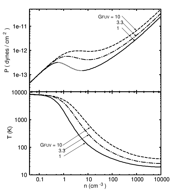
Figure 1: Equilibrium gas temperature and pressure of the neutral medium for a given gas density and FUV radiation field. In each panel, the broken, dotted, and solid lines respectively represent the equilibrium curves with different FUV radiation fields, $G_{\rm FUV}=10$, 3.3, and 1. The dotted curve in the upper panel denotes the thermally-unstable equilibrium states for $G_{\rm FUV}=1$.

We adopt $G_{\rm FUV}=1.0$ as the standard value of the FUV background field, and include no attenuation in the ambient medium. The equilibrium $n$-$P$ and $n$-$T$ curves for $G_{\rm FUV}=1.0$ are presented in Figure 1 (also see Wolfire et al., 1995; Koyama & Inutsuka, 2000). The cooling rate exceeds the heating rate above the equilibrium curve, and vice versa. The thermally unstable equilibrium states for $G_{\rm FUV}=1.0$ are denoted by the dotted lines. As the upper panel of Figure 1 shows, the two thermally stable equilibrium states can coexist under the same gas pressure of $1.5\lesssim P\lesssim 3.2~{}(10^{-13}{\rm dynes/cm}^{2})$, which are the CNM and WNM. The thermal balance is achieved mainly between the photoelectric heating and radiative cooling by [C II] 157.7$\mu$m (Ly-$\alpha$ and [O I] $63.1\mu$m) in the CNM (WNM). In Figure 1, we also plot equilibrium curves with the stronger FUV fields of $G_{\rm FUV}=3.3$ and 10. The equilibrium temperature increases with the stronger FUV field, owing to the efficient photoelectric heating. In our numerical models presented in § 3, the FUV radiation field can be as high as $G_{\rm FUV}>10$ just outside the H II region, owing to the proximal massive star. As shown in § 3.1 below, the SF emerges and a dense shell forms around the H II region expanding in the ambient CNM. These equilibrium curves are useful to interpret the calculated physical states in the shell. We analyze the transition of physical states across the SF with these equilibrium curves in § 3.1.

Table 1. Model Parameters

Model	$M_{*}~{}(M_{\odot})^{a}$	$n_{\rm H,0}({\rm cm^{-3}})^{b}$	$\log S_{\rm UV}({\rm s}^{-1})^{c}$	$\log S_{\rm FUV}({\rm s}^{-1})^{d}$	$R_{\rm st}~{}({\rm pc})^{e}$	$t_{\rm dyn}~{}({\rm Myr})^{f}$
CNM-S64	63.8	10	49.35	49.16	18.16	1.67
CNM-S41	40.9	10	48.78	48.76	11.73	1.08
CNM-S22	21.9	10	48.10	48.33	6.96	0.64
CNM-S18	17.5	10	47.02	47.99	3.04	0.28
CNM-S12	11.7	10	45.38	47.39	0.86	0.08
WNM-S41	40.9	0.1	48.78	48.76	252.7	23.27
WNM-S18	17.5	0.1	47.02	47.99	65.45	6.03
WNM-S12	11.7	0.1	45.38	47.39	18.59	1.71

a : mass of the central star, b : number density of the ambient gas, c : UV-photon number luminosity of the central star, d : FUV-photon number luminosity of the central star, e : initial Strömgren radius, f : dynamical time, $R_{\rm st}/C_{\rm II}$, where $C_{\rm II}$ is the sound speed at a temperature of $T=10^{4}$ K.

We calculate the time evolution of the expanding H II regions in both the CNM and WNM. For the ambient CNM and WNM, we adopt the typical number densities of $n_{\rm H,0}=10~{}{\rm cm}^{-3}$ and $n_{\rm H,0}=0.1~{}{\rm cm}^{-3}$ respectively. The equilibrium temperature and ionization fraction are $106~{}{\rm K}$ and $5.9\times 10^{-4}$ in the CNM, and $7900~{}{\rm K}$ and $2.9\times 10^{-2}$ in the WNM. The time evolution is calculated until 10 Myr in all models. In order to focus on the role of stellar UV and FUV radiation, we do not include other kinetic effects produced by wind-driven bubbles and supernova explosions. We briefly discuss these other dynamical processes in § 5.

3 Results of the Numerical Calculations

3.1 Expansion in Cold Neutral Medium

3.1.1 Fiducial Model : Expansion around $41~{}M_{\odot}$ Star

First, we consider the time evolution around a massive star of $41~{}M_{\odot}$ in the ambient CNM (model CNM-S41) as the fiducial model. Figure 2 shows the hydrodynamical evolution of the H II region and shell in this model. The basic time evolution is the same as that of the H II region in the ambient molecular material (Papers I and II). When the IF passes the initial Strömgren radius ($\sim 10$ pc), the SF emerges in front of the IF. Since the gas temperature of the ambient CNM is only $\sim 100$ K, the H II region ($T\sim 10^{4}$ K) has sufficient excess pressure to drive the SF. The SF sweeps up the ambient CNM, and a dense shell is formed just around the H II region. The time evolution of the expansion is well approximated by,

$$R_{\rm IF}(t)=R_{\rm st}\left(1+\frac{7}{4}\sqrt{\frac{4}{3}}\frac{t}{t_{\rm dyn}}\right)^{4/7}.$$ (1)

The characteristic length scale, $R_{\rm st}$ is the initial Strömgren radius,

$$R_{\rm st}=13.9~{}{\rm pc}~{}\left(\frac{S_{\rm UV}}{10^{49}~{}{\rm s^{-1}}}\right)^{1/3}\left(\frac{n_{0}}{10~{}{\rm cm}^{-3}}\right)^{-2/3},$$ (2)

and timescale, $t_{\rm dyn}$ is the dynamical time,

$$t_{\rm dyn}=R_{\rm st}/C_{\rm II}=1.22~{}{\rm Myr}~{}\left(\frac{S_{\rm UV}}{10^{49}~{}{\rm s^{-1}}}\right)^{1/3}\left(\frac{n_{0}}{10~{}{\rm cm}^{-3}}\right)^{-2/3},$$ (3)

where $S_{\rm UV}$ is the UV-photon number luminosity of the central star, $C_{\rm II}$ is the sound speed in the H II region, and $n_{0}$ is the ambient number density. The gas density in the shell is about 100 times as dense as the ambient CNM. The gas temperature in the shell is only $\sim 30$ K, which is much lower than the ambient temperature. The ambient neutral medium just outside the H II region is slightly warmer than that in the outermost region. This is due to photoelectric heating by the intense FUV radiation from the central star. For example, the FUV flux just outside the SF is $G_{\rm FUV}\sim 10$ at $t\sim 1$ Myr. Because of the geometrical dilution, the FUV field outside the SF gradually decreases as the HII region expands.

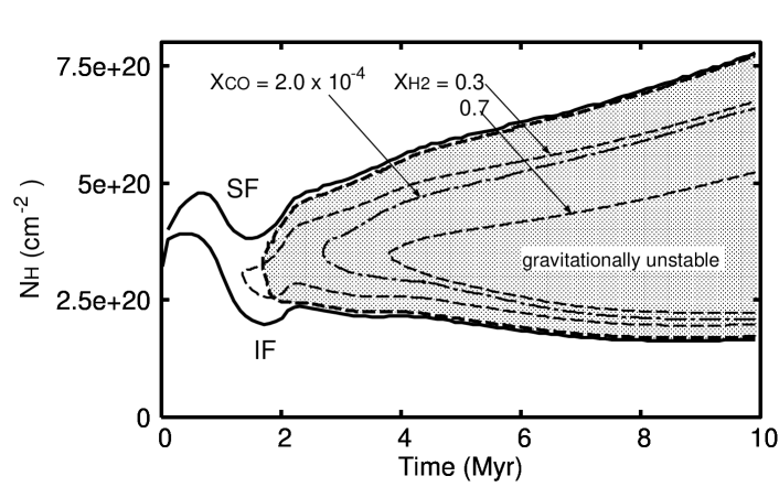
Figure 3: Time evolution of the column density of each region in model CNM-S41. The vertical axis represents the column density of the hydrogen nucleon from the central star, and horizontal axis represents the elapsed time of the calculation. Two thick solid lines correspond to the positions of the SF and IF, and the region enclosed between these lines corresponds to the shell. Although the radius of the IF monotonically increases, the column density of the H II region decreases owing to the decrease of the density. Thin contour curves represent the chemical abundance in the shell; positions where $X_{\rm H_{2}}\equiv 2n_{\rm H_{2}}/n_{\rm H_{nuc}}=0.3$ and 0.7 (broken), and $X_{\rm CO}\equiv n_{\rm CO}/n_{\rm C_{nuc}}=2.0\times 10^{-4}$ (dot-solid). The shaded region denotes the gravitationally unstable region, where $t>(G\rho)^{-0.5}$.

Figure 3 shows the time evolution of the chemical structure of the shell. The hydrogen molecules gradually accumulate in the shell, owing to the rapid reformation on the surface of dust grains. About 45% of hydrogen atoms within the shell exist as H₂ molecules at $t\sim 4.5$ Myr, which is about the lifetime of the adopted main-sequence star. On the other hand, carbon monoxide molecules hardly form in the shell. The reason for this difference is that in this model, the column density of the shell is only $N_{\rm sh}\sim 2.5-5\times 10^{20}~{}{\rm cm}^{-2}$, which corresponds to A${}_{\rm V}\sim 0.125-0.25$. This means that the incident FUV radiation is not significantly attenuated by the dust absorption in the shell. Since the dust absorption does not work, the reformed molecules are protected against FUV photons only by the self-shielding effect. In the equilibrium photodissociation region (PDR) where the self-shielding is dominant over the dust absorption, the column density of the hydrogen nucleon between the IF and H₂ dissociation front (DF) is,

$$N_{\rm DF}\sim 5\times 10^{20}~{}{\rm cm}^{-2}\left(\frac{\chi}{0.04}\right)^{4/3},$$ (4)

where $\chi\equiv G_{\rm FUV}/n$ (Hollenbach & Tielens, 1999). For the accumulation of H₂ molecules in the shell, $N_{\rm DF}$ must be smaller than the column density of the shell, which corresponds to $\chi\leq 2-4\times 10^{-2}$. In our calculation, $\chi$ is always only a few $\times 10^{-3}$ at the IF (see also Figure 7), and the reformed H₂ molecules are reliably self-shielded in the shell. In addition to the sufficient self-shielding in the equilibrium state, the H₂ reformation timescale is sufficiently short in the shell. The reformation time is given by

$$t_{\rm form}\sim 100~{}{\rm Myr}~{}\left(\frac{n}{10~{}{\rm cm}^{-3}}\right)^{-1}$$ (5)

(e.g., Hollenbach et al., 1971), and $t_{\rm form}\sim 1$ Myr in the shell. Therefore, equilibrium H₂ abundance is achieved during the expansion. On the other hand, the self-shielding of CO molecules is inefficient owing to the small abundance of carbon and oxygen atoms. Even if H₂ molecules can accumulate in the shell, CO molecules cannot form without sufficient $N_{\rm sh}$ for shielding FUV photons by the dust absorption (Bergin et al., 2004, Paper II). The shielding by H₂ molecules is an effect secondary to the dust shielding. These features do not change in the H I clouds with $n_{\rm H,0}\sim$ a few $\times 10~{}{\rm cm}^{-3}$, but change in the molecular clouds, where the ambient number density is high, $n_{\rm H,0}\geq 100~{}{\rm cm}^{-3}$. This is well understood with the $n$-dependence of the column density of the shell, $N_{\rm sh}$ and the incident FUV flux at the IF, $F_{\rm FUV,i}$ at a given $t/t_{\rm dyn}$,

$$N_{\rm sh}\propto nR_{\rm st}\propto n^{1/3},$$ (6)

$$F_{\rm FUV,i}\propto S_{\rm FUV}/R_{\rm st}^{2}\propto n^{4/3}.$$ (7)

As equation (6) shows, the column density of the shell rises with the higher ambient number density. Although equation (7) shows that the incident FUV flux also increases with increasing $n$, the intense FUV radiation can be shielded. Since the dust attenuation works as $\exp(-\tau_{d})$, the dust shielding effect quickly becomes significant once the dust opacity of the shell, $\tau_{d}~{}(\propto N_{\rm sh})$ exceeds unity. When the H II region sufficiently expands in the molecular cloud, therefore, the FUV radiation can be blocked by the dust absorption, and both H₂ and CO molecules can accumulate in the shell (see Papers I and II).

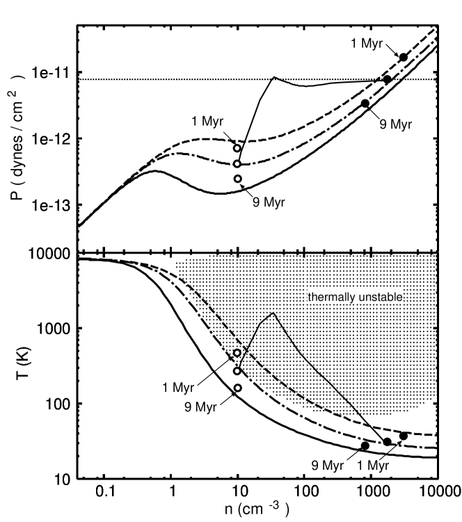
Figure 4: The radiative equilibrium states shown on the n-P (upper panel) and n-T (lower panel) planes. Solid, dot-solid, and broken lines represent the radiative equilibrium curves for different FUV fields, $G_{\rm FUV}=1$, 3.3, and 10 respectively. In each panel, “$\circ$”(“$\bullet$”) signs indicate the calculated states in the pre-shock (post-shock) region at $t=1$, 3 and 9 Myr in model CNM-S41. In the upper panel, the dotted line indicates $P_{\rm ram}$ at $t=3$ Myr calculated by equation (12). The evolutionary track across the SF at $t\sim 3$ Myr is shown by thin solid line in each panel. In the lower panel, the shaded region denotes where the isobarically contracting and cooling layer is expected to be thermally unstable by the linear stability analysis (see text).

In our calculation, the swept-up CNM ($T\sim 100$ K) is converted to the cold ($T\sim 30$ K) partially atomic and molecular gas behind the SF. The formation mechanism of such a dense and cold shell is not understood within the framework of the isothermal SF. Furthermore, Figure 2 shows that the shell density and temperature gradually decrease as the H II region expands. We can understand all these features with the equilibrium $n$-$P$ and $n$-$T$ curves of the neutral medium. In Figure 4, “$\circ$” signs represent the physical states in the pre-shock region at $t=1,3$, and 9 Myr in our numerical simulation. This figure shows that “$\circ$” sign vertically goes down with increasing time $t$, which means that the pre-shock temperature and pressure decrease almost isochorically. This is because the FUV radiation field just outside the shell gradually diminishes owing to the geometrical dilution, so that the photoelectric heating becomes inefficient. Since the heating timescale is much shorter than the dynamical timescale, $t_{\rm dyn}\sim 1$ Myr, the thermal equilibrium is achieved at each time step. In the same figure, “$\bullet$” signs represent physical states in the post-shock region at each snapshot. The upper panel shows that the gas pressure increases by about ten times across the SF. We can understand this high post-shock pressure by recalling the derivation of equation (1). Equation (1) is derived from the equation of motion of the shell,

$$M_{\rm sh}\ddot{R}_{\rm IF}=4\pi R_{\rm IF}^{2}(P_{\rm II}-P_{\rm ram})$$ (8)

(Paper II). In this equation, $M_{\rm sh}$ is the mass of the swept-up shell,

$$M_{\rm sh}=\frac{4\pi}{3}\rho_{0}R_{\rm IF}^{3},$$ (9)

$P_{\rm II}$ is the thermal pressure in the H II region,

$$P_{\rm II}=\rho_{0}C_{\rm II}^{2}\left(\frac{R_{\rm st}}{R_{\rm IF}}\right)^{3/2},$$ (10)

$P_{\rm ram}$ is the ram pressure,

$$P_{\rm ram}=\rho_{0}\dot{R}_{\rm IF}^{2},$$ (11)

and $\rho_{0}$ is the ambient mass density. As equation (8) shows, the motion of the shell is controlled by the balance between the thermal and ram pressure from the inner and outer edge of the shell. Using equations (1), (10) and (11), the ram pressure can be written as,

$$P_{\rm ram}=\frac{4}{3}\rho_{0}C_{\rm II}^{2}\left(1+\frac{7}{4}\sqrt{\frac{4}{3}}\frac{t}{t_{\rm dyn}}\right)^{-4/7}=\frac{4}{3}P_{\rm II}.$$ (12)

The backward ram pressure is always greater than the forward thermal pressure by a factor of $4/3$, and the expansion is decelerating. Since the sound crossing time of the shell is much shorter than $t_{\rm dyn}$, the pressure within the shell smoothly connects with $P_{\rm ram}$ ($P_{\rm II}$) at the outer (inner) edge of the shell. Therefore, the post-shock pressure is almost equal to $P_{\rm ram}$ at each time step. The pressurized neutral medium is not initially in the thermal equilibrium state, but going to the equilibrium state over the cooling timescale, $t_{\rm cool}$. Since $t_{\rm cool}\sim 0.1$ Myr is much shorter than $t_{\rm dyn}$, the gas element engulfed in the shell quickly reaches the thermal equilibrium state. Figure 4 shows that the calculated density and temperature in the post-shock region are equal to the equilibrium values for the given post-shock pressure ($\sim P_{\rm ram}$) and FUV field at each time step.

While the gas element is going to the new equilibrium state, the total cooling rate significantly exceeds the heating rate. The dominant cooling process for this non-equilibrium gas is the line cooling of CII (157.7$\mu$m). The frequency-integrated emergent intensity of this line emission is about,

$$I_{\rm ne}\sim\frac{1}{8\pi}\rho_{0}v_{\rm sh}^{3}=0.9\times 10^{-6}\left(\frac{n_{\rm H,0}}{10~{}{\rm cm}^{-3}}\right)\left(\frac{v_{\rm sh}}{10~{}{\rm km/s}}\right)^{3}\quad{\rm ergs/cm^{2}/sec/str}$$ (13)

(Hollenbach & McKee, 1979), where $\rho_{0}$ is the ambient mass density, and $v_{\rm sh}$ is the shock velocity. As equation (13) shows, the emission from the non-equilibrium cooling layer quickly diminishes as the shell decelerates. Besides the non-equilibrium cooling layer just behind the SF, most of the gas within the shell is in the thermal equilibrium state, where the photoelectric heating is mainly balanced by the CII (157.7$\mu$m) line cooling. Therefore, the CII line emission also comes from the shell itself. The emergent intensity from the equilibrium shell is about,

$$I_{\rm e}\sim\frac{1}{2\pi}\overline{\Lambda_{\rm CII}}N_{\rm sh}=1.6\times 10^{-6}\left(\frac{\overline{\Lambda_{\rm CII}}}{10^{-25}{\rm ergs/sec}}\right)\left(\frac{N_{\rm sh}}{10^{20}~{}{\rm cm}^{-2}}\right)\quad{\rm ergs/cm^{2}/sec/str},$$ (14)

where $\overline{\Lambda_{\rm CII}}$ is the average CII cooling rate in the shell. As expected from equations (13) and (14), the total CII emission is dominated by that from the shell in the thermal equilibrium, but for the very early phase of the expansion. Although this far-IR CII emission could be detected, this line, an ordinary feature of the PDR, is not a good signpost of the molecular cloud formation. Instead, we seek the predicted gas phase using the HISA feature in § 4.

In our 1-D calculation, the neutral medium is steadily swept up into the shell. However, some instabilities actually deform the shell and excite its internal structure. First, the dense gas layer is expected to fragment by the gravitational instability. The shell-fragmentation occurs first at the length scale of the layer thickness, with a growth timescale of $\sim(G\rho)^{-1/2}$ (e.g., Elmegreen & Elmegreen, 1978; Miyama, Narita & Hayashi, 1987; Nagai, Inutsuka & Miyama, 1998). We adopt $t>(G\rho)^{-1/2}$ as the simplified criterion of the gravitationally unstable layer. Figure 3 shows that the shell becomes gravitationally unstable soon after $t\sim 2$ Myr, when H₂ molecules begin to accumulate in the shell. The typical radius and mass of the fragment are about 0.1 pc and $10~{}M_{\odot}$ respectively. If each fragment subsequently contracts, the molecular reformation will be promoted by the self-shielding of cores, owing to the increased column density. Second, the compressed layer collapsing due to the significant radiative cooling just behind the SF, suffers from thermal instability (Koyama & Inutsuka, 2000, 2002). In Figure 4, we plot the evolution track of a fluid element across the SF at $t\sim 3$ Myr. The gas temperature rises up to $T\sim 2000$ K at the SF, due to compressional heating, and falls to $T\sim 30$ K, due to the significant radiative cooling behind the SF. The timescale to settle into the new equilibrium state is about the cooling time, $t_{\rm cool}\sim 0.1$ Myr. The upper panel of Figure 4 shows that the collapsing layer evolves almost isobarically. The linear stability analysis of the isobarically collapsing layer has been explored by Koyama & Inutsuka (2000), and the shaded region in the lower panel of Figure 4 represents the expected thermally unstable region with $G_{\rm FUV}=3.3$. Note that the gas is cooling and isobarically contracting in the unperturbed state in their linear analysis. Whether the small perturbation grows or not is analyzed in the evolving background state, which differs from the original analysis by Field (1965). Figure 4 shows that the compressed CNM becomes thermally unstable on its way to the new equilibrium state. The linear analysis shows that the layer fragments into tiny cloudlets, whose size is about tens of AUs, over the timescale of $10^{3-4}$ yr (Koyama & Inutsuka, 2000). Multi-dimensional numerical simulations (e.g., Koyama & Inutsuka, 2002; Audit & Hennebelle, 2005) show that each fragment has some translational motion of a few km/s. This motion is driven by the pressure of the surrounding warmer, less dense region. Thus, the motion is inevitably subsonic for the surrounding medium, and does not dissipate over the sound-crossing time. Koyama & Inutsuka (2002) have suggested that this translational cloudlets motion is the origin of the observed broad line width, or “turbulence” in the cold clouds. Our current 1-D calculations cannot explain the the actual evolution of the fragmentation of the shell, which will be affected by both the thermal and gravitational instabilities. Future multi-dimensional simulations of radiative-hydrodynamics will reveal the detailed nature of the fragmented shell.

3.1.2 Dependence on Central Stars

Second, we study how time evolution changes with different central stars in the same ambient CNM. Our numerical results show a clear feature; with the higher-mass central star, the shell density is higher and the reformation of H₂ molecules becomes more efficient in the shell.

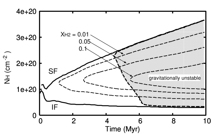
Figure 6: Same as Figure 3 but for model CNM-S18. The contours with thin broken curves represent the positions where $X_{\rm H_{2}}=0.01$, 0.05 and 0.1 respectively.

For example, Figure 5 presents gas-dynamical evolution around a massive star of $M_{*}=11.7~{}M_{\odot}$ (model CNM-S12). The SF emerges and sweeps up the ambient CNM, which is the same as model CNM-S41. The shell density is 10 times as high as the ambient CNM density at $t\sim 1$ Myr, but quickly declines afterward. The shell density is always lower than that in model CNM-S41 at the same time, $t$ (c.f. Figure 7). Despite the different densities of the shells, the temperature profiles in Figures 2 and 5 are similar. This is because the FUV field outside the shell is similar among these models (Figure7). The FUV flux just outside the SF is $G_{\rm FUV}\sim 10$ at $t\sim 1$ Myr, and gradually decreases owing to the geometrical dilution. The formation of molecules in the shell hardly occurs in model CNM-S12. No CO molecules are formed, and only less than 0.1% of H atoms is converted to H₂ molecules in the shell over 10 Myr. Since the column density of the shell is $N_{\rm sh}<2.5\times 10^{20}~{}{\rm cm}^{-2}$, the dust absorption does not protect reformed molecules against FUV photons. As shown in equation (4), the self-shielding becomes less efficient with the larger $\chi=G_{\rm FUV}/n$ in the shell. In model CNM-S12, $\chi$ is about ten times as large as that in model CNM-S41 at the same time, $t$ (also see Figure 7). Therefore, $N_{\rm DF}$ given by equation (4) exceeds the column density of the shell, and even the self-shielding of H₂ molecules does not work. Furthermore, if the self-shielding were efficient, H₂ molecules would not form in the low-density shell. Equation (5) shows that the reformation timescale becomes longer than 10 Myr, when the shell density is smaller than $100~{}{\rm cm}^{-3}$. The reformation timescale is so long that no equilibrium H₂ abundance is achieved. We have calculated other models with different exciting stars, and found that the formation of H₂ molecules is more efficient with higher-mass stars. Figure 6 shows the time evolution of the chemical structure of the shell around the central star of $17.5~{}M_{\odot}$ (model CNM-S18). In this model, H₂ molecules are slightly formed in the shell. About 6 % of swept-up hydrogen atoms are converted to H₂ molecules by the time of 10 Myr.

We investigate why the efficiency of H₂ formation depends on the mass, or UV/FUV luminosity of the central star. The key physical quantities are the ratio, $\chi=G_{\rm FUV}/n$ and number density, $n$, in the shell. The former reflects the efficiency of the self-shielding effect, which determines the H₂ abundance in the equilibrium state, and the latter determines the reformation timescale, over which the H₂ abundance becomes the equilibrium value. Figure 7 shows the time evolution of the number density, FUV radiation field, and their ratio, $\chi$ in the shell in models CNM-S41, S18, and S12, respectively. At the same time, $t$, the number density is larger with higher-mass stars, and the FUV fields are similar among models. Thus, their ratio, $\chi$ is smaller with a higher-mass star. The self-shielding effect is more efficient with a higher-mass central star, as equation (4) shows. The higher shell density ensures that the equilibrium state is achieved over a shorter timescale, and that H₂ molecules quickly accumulate in the shell with a higher-mass star. Consequently, the variation in the chemical structure of the shell originates in similar and different time evolutions of $G_{\rm FUV}$ and $n$ among models shown in Figure 7.

We make use of some analytic relations to interpret these characteristic features. First, the FUV field at time $t$, $G_{\rm FUV}(t)$ scales with the UV/FUV luminosity of the star,

$$G_{\rm FUV}(t)\propto\frac{S_{\rm FUV}}{R_{\rm IF}(t)^{2}}\propto S_{\rm FUV}^{1/3}\left(\frac{S_{\rm FUV}}{S_{\rm UV}}\right)^{2/3}\left(1+\frac{7}{4}\sqrt{\frac{4}{3}}\frac{t}{t_{\rm dyn}}\right)^{-8/7}.$$ (15)

This shows that $G_{\rm FUV}(t)$ is normalized with the first term, $S_{\rm FUV}^{1/3}(S_{\rm FUV}/S_{\rm UV})^{2/3}$, which is smaller with the more massive star. On the other hand, the last evolutionary term has an inverse dependence, because the dynamical time, $t_{\rm dyn}$ is longer with the higher-mass star (see equation (3)). Owing to the cancellation of these opposite dependences, the time evolution of the FUV field is similar among models with different stars, as shown in Figure 7.

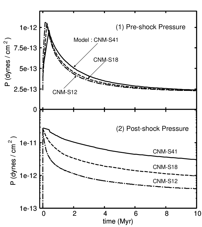
Figure 8: Time evolution of the gas pressure in the pre-shock and post-shock regions. The solid, broken, and dot-solid lines in each panel represent the evolution of models CNM-S41, S18, and S12 respectively.

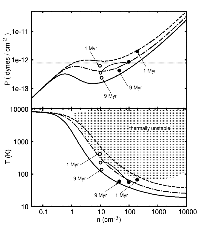
Figure 9: Same as Figure 4 but for model CNM-S12.

Next, let us consider why the shell density is larger with a higher-mass star. In § 3.1.1, we have shown that the post-shock density is determined by the FUV radiation field and gas pressure in the shell at each time step. Because of the similarity in the time evolution of $G_{\rm FUV}$ among models, only gas pressure in the shell dominates the post-shock physical state. The time evolution of the ram pressure is given by equation (12), where the dynamical time, $t_{\rm dyn}$ is longer with the higher-mass star. Therefore, thermal pressure in the shell is higher with the higher-mass star at the same time, $t$, which causes a variation in shell density among models. Figure 8 presents the time evolution of thermal pressure in both pre-shock and post-shock regions in models CNM-S41, S18, and S12. Since the FUV radiation field is similar, the time evolution of the pre-shock pressure is almost the same among models. The post-shock pressure is higher with the higher-mass star, as predicted by equation (12). The significant enhancement of the pressure behind the SF accounts for the high density of the shell. Figure 9 presents several post-shock and pre-shock physical states in model CNM-S12. In this model, the post-shock pressure is just a little higher than the pre-shock pressure, and the shell density is significantly lower than that in model CNM-S41 (c.f. Fig. 4).

Finally, we discuss the multi-dimensional structure of the shell expected to be produced by various instabilities. First, gravitational instability grows earlier in denser layers. Since the shell density is higher with a higher-mass star, shell-fragmentation will occur earlier in these higher-mass models. While the shell becomes unstable at $t\sim 2$ Myr in model CNM-S41 (Figure 3), it is not until $t\sim 5$ Myr that the unstable region appears in model CNM-S18 (Figure 6). No gravitationally unstable region appears in CNM-S12. Second, the thermal stability of the isobaric cooling layer depends on the compression level across the SF. Figure 9 shows the evolution track of the layer at $t\sim 3$ Myr in model CNM-S12. The pressure rises by a factor of two or three across the SF, and the evolution track only grazes the thermally unstable region on the $n$-$T$ plane. In summary, our calculations show that H₂ formation is more efficient in a model with a higher-mass star, and that the effects of gravitational/thermal instability are more significant in such higher-mass models.

3.2 Expansion in Warm Neutral Medium

Once the stellar UV radiation escapes from the molecular clouds and H I clouds (CNM), the H II region expands to the WNM. Figure 10 shows the hydrodynamical evolution of the H II region around a $41~{}M_{\odot}$ star in the ambient WNM (model WNM-S41). Because of the low ambient number density, the H II region expands into a very large region of more than $100$ pc. As Figure 10 shows, however, the expanding H II region hardly affects the hydrodynamics. The gas density slightly increases by a factor of two in front of the IF. This is partly because of the large initial Strömgren radius. In model WNM-S41, the initial Strömgren radius is, $R_{\rm st}\sim 250$ pc, and the H II region remains in its early formation phase at $t\lesssim 2$ Myr. Furthermore, after the H II region reaches the initial Strömgren radius, no dense shell is formed around the H II region. The ambient gas temperature is originally as high as $T\sim 8000$ K, and the pressure excess of the H II region over the ambient WNM is small. No SF with a high Mach number ever emerges in front of the IF. The ambient WNM is only converted to the ionized medium with a similar temperature and density, which is the WIM. These basic features of the time evolution do not change with different central stars. Although Hennebelle & Pérault (1999) and Koyama & Inutsuka (2000) have shown that the highly pressurized WNM can be converted into the CNM, this is not the case with the expanding HII regions. The bubble driven by stellar-wind or supernova explosion can provide the much higher pressure even in the WNM, and triggers the phase transition from WNM to CNM (also see § 5.3).

4 Hunt of the Dark Molecular Hydrogen Clouds in the Observational Data

4.1 Shell-like HI Self-absorption around Giant H II Regions

When the H II region expands in the CNM, the SF emerges in front of the IF and the ambient CNM is compressed in the shell. We have shown that H₂ molecules can form if the central star is more massive than $18~{}M_{\odot}$, but CO molecules seldom form in the shell. The calculated temperature and density in the shell are $T\sim$ a few $\times$ 10 K and $n\sim 100-1000~{}{\rm cm}^{-3}$. This is just the gas phase intermediate between the ambient CNM and molecular clouds observed with the CO emission. However, it is generally difficult to detect such an intermediate gas phase. The gas temperature is too low to thermally excite the rovibrational transition of H₂ molecules. The FUV radiation field in the shell is $G_{\rm FUV}\sim 10$ at most, and it is hard to detect the UV fluorescent H₂ emission from the distant giant H II regions. Instead of hunting for signs of the cold H₂ molecules, we probe the predicted “dark” hydrogen with the H I self-absorption (HISA). The HISA is the H I 21-cm line-absorption against the background emission from the warmer neutral medium. Statistical studies of the CNM usually analyze the distribution of the 21-cm absorption features against the strong radio continuum sources, such as compact H II regions and supernova remnants (e.g., Dickey et al., 2003; Heiles & Troland, 2003a, b). On the other hand, the brightness temperature of the background H I 21-cm emission is only $T_{\rm b}\sim 100$ K, and HISA features automatically trace the colder tail of the CNM.

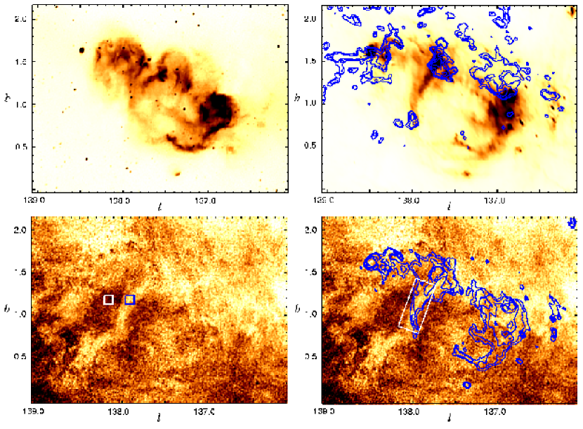
Figure 11: Multi-wavelength view of the W5 region using CGPS data. Upper left : image of the 21-cm continuum emission (H II gas). The brightness temperature is linearly scaled from 5 K (bright) to 12.5 K (dark). Upper right : image of the 60-$\mu$m dust emission and contours of ¹²CO(1-0) line emission at $v_{\rm LSR}=-39.8$ km/s. The intensity of the 60-$\mu$m dust emission is linearly scaled from 10 MJy/str (bright) to 200 MJy/str (dark). The contour levels of CO emission are $T_{\rm b}=1,2,5$, and 10 K. Lower left : channel map of the H I 21-cm emission at $v_{\rm LSR}=-39.8$ km/s. The brightness temperature is linearly scaled from 45 K (bright) to 110 K (dark). The blue (white) $6^{\prime}\times 6^{\prime}$ square denotes the on-region (off-region) used for the analysis. Lower right : channel map of the H I 21-cm emission at $v_{\rm LSR}=-39.8$ km/s and contours of 60-$\mu$m dust emission. The contour levels are $I_{\rm 60\mu m}=75,92.2,143.8,230$ and 350 MJy/str. The region enclosed by the white line denotes where the HISA feature shows the good spatial correlation with the dust shell.

We have sought the HISA features associated with the giant H II regions using recent observational data by the Canadian Galactic Plane Survey (CPGS; see Taylor et al., 2003). The CGPS data provides us with the high-resolution ($\sim 1^{\prime}$) maps of HII, HI, CO, and dust in the Galactic plane. We use the 21-cm continuum image and velocity cube of the 21-cm emission by the Dominion Radio Astrophysical Observatory (DRAO) survey (Higgs & Tapping, 2000), ¹²CO(1-0) data cubes by the Five College Radio Astronomy Observatory (FCRAO) outer galactic survey (Heyer et al., 1998), and reprocessed IRAS images at 60 and $100~{}\mu$m bands (Cao et al., 1997). We have examined the star-formation complex W3-W4-W5 along the Perseus arm, which includes the giant H II regions, W3, W4 and W5. Adopting a distance of $1.95$ kpc to the Perseus arm (Xu et al., 2006), the angle of $1\arcdeg$ corresponds to 32.2 pc. Figure 11 shows the multi-wavelength view of the W5 region. The upper left panel is the 21 cm continuum map, which shows distribution of ionized hydrogen. The upper-right panel presents a $60~{}\mu$m image of the W5 region, and we can see the clear shell-like structure around the ionized gas. Other IRAS-band images also show similar shell-like structures (Karr & Martin, 2003). The lower left panel of Figure 11 shows a channel map of 21-cm emission at $v_{\rm LSR}=-39.8$ km/s. We have also found a narrow shell-like feature in this map, which shows strong spatial correlation with the dust shell, as indicated by the white rectangle in the lower right panel. The brightness temperature along the shell-like feature is $T_{\rm b}\sim 70$ K, which is lower than that on both sides of the shell, $T_{\rm b}\sim 100$ K. Since it is very unlikely that the 21-cm emission from the diffuse WNM would fluctuate over such a small scale, and that such fluctuation would overlap with the dust shell by accident, we consider this shell-like feature as being HISA by the colder neutral medium. Furthermore, these dust shell and shell-like HISA feature should originate in the same structure just around the W5 H II region. We also show the contours of the ¹²CO(1-0) channel map at the same velocity in the upper right panel, but the CO emission does not trace the shell-like structures with the current sensitivity of the FCRAO survey.

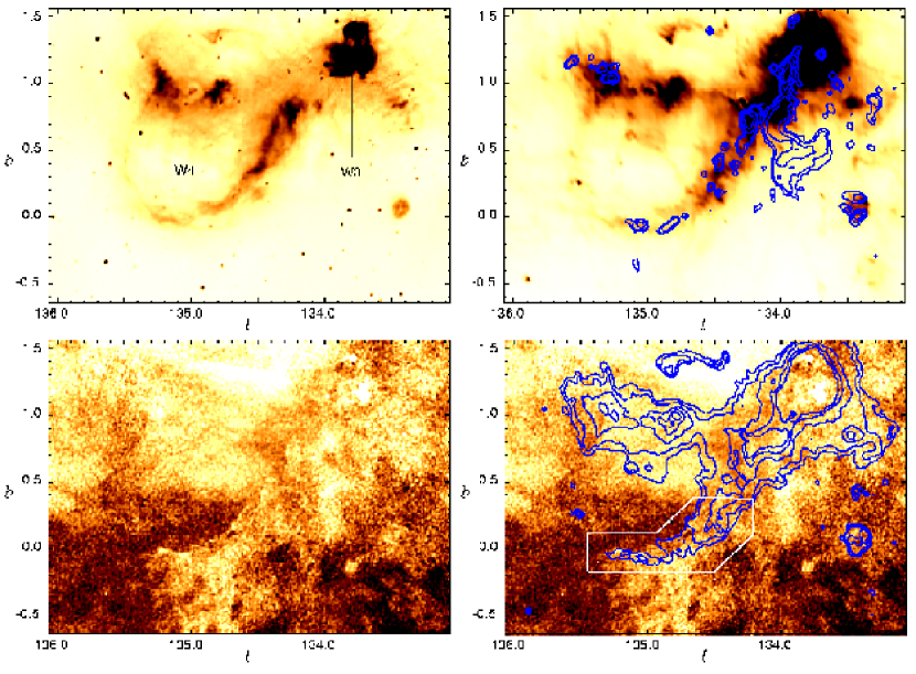
Figure 12: Multi-wavelength view of the W3-W4 region using CGPS data. The distribution of panels and the scaling of images and contours are almost the same as those in Figure 11. Some differences are as follows: Upper left : The brightness temperature is linearly scaled from 4.9 K (bright) to 20.0 K (dark). Lower right : The contour levels of the 60-$\mu$m intensity of the dust emission are $I_{\rm 60\mu m}=65,82.8,136.3,225.3$, and 350 MJy/str. The channel maps of ¹²CO(1-0) and H I 21 cm emission are at $v_{\rm LSR}=-47.3$ km/s. The region enclosed by the white line denotes where the HISA feature shows the good spatial correlation with the dust shell.

We have also found some similar features in the giant H II region, W4. Figure 12 shows a multi-wavelength view of the W3-W4 region. The upper left panel shows the distribution of the ionized hydrogen. The W4 H II region has an ionized shell-like structure. The W3 H II region is denser and more compact than W4. The upper right panel presents the $60~{}\mu$m image superposed on the contours of the ¹²CO(1-0) channel map at $v_{\rm LSR}=-47.3$ km/s. The distributions of both the dust and CO emission are two-fold. In $l\gtrsim 134.3\arcdeg$, the $60~{}\mu$m emission shows a shell-like structure just outside the ionized shell. The CO molecules are also along the dust shell, but discretely distributed as small clouds. In $\l\lesssim 134.3\arcdeg$, on the other hand, the broad and strong $60~{}\mu$m emission comes from the warmer dust around the W3 H II region. The CO emission also broadly extends in $\l\lesssim 134.3\arcdeg$. This is the eastern edge of the W3 giant molecular cloud (GMC), which actually extends over $l<133\arcdeg$. The lower-left panel of Figure 12 shows the 21-cm channel map at $v_{\rm LSR}=-47.3$ km/s. The HISA feature has also been found, and overlaps with the dust shell (lower-right panel). Carpenter, Heyer & Snell (2000) have shown that the small molecular clouds are widely distributed in the W3-W4-W5 cloud complex, and have speculated that these are remnants of pre-existing molecular clouds dispersed by the negative feedback from massive stars. We suggest that a number of the small clouds form from the compressed ambient neutral medium.

4.2 Quantitative Analysis of the Data

In order to constrain the physical state of the observed HISA cloud, we quantitatively analyze the data. We define “on”- and “off”-regions designated by $6^{\prime}\times 6^{\prime}$ squares in the lower-left panel of Figure 11. The on-region is just on the HISA feature around the W5 H II region, and the off-region is slightly outside the HISA feature. Figure 13 presents the averaged brightness temperatures in the on-region ($T_{\rm on}$) and off-region ($T_{\rm off}$) at different velocities. The emission profile in the on-region clearly shows a depression compared with that in the off-region. We regard this absorption feature as the HISA profile, and obtain the line profile calculating $T_{\rm on}-T_{\rm off}$. The line depth and width are about $\Delta T\sim 30$ K, and $\Delta v\sim 5$ km/s respectively. The velocity at the line center is $v_{\rm LSR}\sim-40$ km/s, which is the velocity of the channel maps presented in Figure 11. The HISA profile is available to limit $T_{\rm HISA}$ and $\tau_{\rm HISA}$ considering the radiative transfer under a given geometry of the system (e.g., Gibson et al., 2000). We suppose that the HISA cloud, whose spin temperature and optical depth are $T_{\rm HISA}$ and $\tau_{\rm HISA}$, lies in the sea of the WNM. The diffuse WNM is distributed in both the foreground and background of the HISA cloud. The spin temperature and the optical depth of the foreground (background) WNM are represented as $T_{\rm fg}$ ($T_{\rm bg}$) and $\tau_{\rm fg}$ ($\tau_{\rm bg}$). Note that the spin temperature of the WNM differs from the kinetic temperature by a factor of two or three, because the thermal equilibrium is not achieved owing to its low density, $n\sim 0.1~{}{\rm cm}^{-3}$ (e.g., Liszt, 2001). The continuum radiation includes the free-free emission from the H II region, cosmic microwave background and so on. In our case, the W5 H II region is so diffuse that the brightness temperature of the continuum radiation, $T_{\rm c}$, is much smaller than that of the line emission. Presuming that all the gas components except the HISA cloud are optically thin, the radiative transfer equation along the line of sight in the on- and off-region are,

$$T_{\rm on}=\tau_{\rm fg}T_{\rm fg}+T_{\rm HISA}(1-e^{-\tau_{\rm HISA}})+\tau_{\rm bg}T_{\rm bg}e^{-\tau_{\rm HISA}}+T_{\rm c}e^{-\tau_{\rm HISA}}-T_{\rm c},$$ (16)

$$T_{\rm off}=\tau_{\rm fg}T_{\rm fg}+\tau_{\rm bg}T_{\rm bg},$$ (17)

where $T_{\rm on}$ ($T_{\rm off}$) is the brightness temperature observed in the on- (off-) region. Subtracting equation (17) from equation (16), we obtain,

$$T_{\rm on}-T_{\rm off}=(1-e^{-\tau_{\rm HISA}})(T_{\rm HISA}-pT_{\rm off}-T_{\rm c})$$ (18)

(e.g., Gibson et al., 2000; Kavars et al., 2003; Kerton, 2005), where $p$ is the ratio of the background WNM emission to the total emission, $p\equiv\tau_{\rm bg}T_{\rm bg}/T_{\rm off}$. We derive the relation between $T_{\rm HISA}$ and $\tau_{\rm HISA}$ for a given $p$ from equation (18), because $T_{\rm on}$, $T_{\rm off}$ and $T_{\rm c}$ are all observable quantities. We adopt the numerical values of $T_{\rm on}=67.9$ K, $T_{\rm off}=97.3$ K at the line center, and $T_{\rm c}=9.1$ K. In Figure 14, the solid lines represent the $T_{\rm HISA}$-$\tau_{\rm HISA}$ relations with these values for a given $p$. As this figure shows, we can set the maximum spin temperature of the HISA cloud as $T_{\rm HISA}\leq 77$ K, where the equality is satisfied when $p=1$. Inversely, if the foreground WNM emission accounts for more than 25% (50%) of the total WNM emission, which corresponds to $p<0.75$ (0.5), the spin temperature should be lower than 52.7 K (28.3 K). The estimated temperature is comparable to the temperature predicted by our calculations, and much lower than that of the typical PDR, $T\sim 100-1000$ K (Hollenbach & Tielens, 1999, Papers I and II).

We can set further constraint on the $T_{\rm HISA}$-$\tau_{\rm HISA}$ plane using the equation

$$\tau_{\rm HISA}=5.2\times 10^{-19}\frac{N_{\rm HI}}{\Delta v~{}T_{\rm HISA}}$$ (19)

(Dickey & Lockman, 1990), where $N_{\rm HI}$ is the column density of atomic hydrogen in the HISA cloud. The line width, $\Delta v$ is about 5 km/s from the line profile presented in Figure 13. Therefore, another $T_{\rm HISA}$-$\tau_{\rm HISA}$ relation is obtained by equation (19) evaluating $N_{\rm HI}$. Taking into account that the HISA cloud can be partially molecular, the atomic column density is written as $N_{\rm HI}=fN_{\rm H}$, where $N_{\rm H}$ is the total column density of all the hydrogen nuclei and $f$ is the atomic fraction in the HISA cloud. We evaluate the total column density in two different ways, instead of directly measuring the atomic column density. First, we use the extinction map given by Dobashi et al. (2005). They have analyzed the database of the Digitized Sky Survey I (Lasker, 1994) using the star count technique, and completed an extinction map of the entire the Galactic plane. We extract the $A_{\rm V}$ map at $6^{\prime}$ angular resolution around the W5 region. In order to estimate the extinction only through the HISA cloud, we calculate the average extinctions in the on- and off-regions, and derive their difference. The excess extinction in the on-region is $A_{\rm V}=0.81$, which corresponds to $N_{\rm H}\sim 1.6\times 10^{21}~{}{\rm cm}^{-2}$. With this value of $N_{\rm H}$, we plot the $T_{\rm HISA}$-$\tau_{\rm HISA}$ relation given by equation (19) for $f=1.0$, 0.1 and 0.01 in Figure 14. In § 3.1.1 and 3.1.2, our numerical models have predicted that the gas phase of $f\sim 0.5$ and $T\sim$ a few $\times 10$ K should form around the H II region. Figure 14 shows that such a gas phase is still possible under our constraints. Second, let us evaluate the total column density in another way, using the 60- and $100-{\rm\mu m}$ dust emissions (e.g, Arce & Goodman, 1999). The intensity of the thermal and optically-thin dust emission is given by,

$$I_{\lambda}=\tau_{\lambda}B_{\nu}(T_{\rm d}),$$ (20)

where $\tau_{\lambda}$ is the dust opacity, $B_{\nu}$ is the Planck function, and $T_{\rm d}$ is the dust thermal temperature. The dust opacity is written as,

$$\tau_{\lambda}=\epsilon_{\lambda}N_{\rm H},$$ (21)

where $\epsilon_{\lambda}$ is the dust emissivity per hydrogen atom, which is usually expressed as $\epsilon_{\lambda}=\epsilon_{0}\lambda^{-\beta}$. Although $\beta$ and $\epsilon_{0}$ actually vary with the different environments (e.g., Dupac et al., 2003), we adopt the typical emissivity law in the local ISM,

$$\epsilon_{\lambda}=1.0\times 10^{-25}\left(\frac{\lambda}{250~{}{\rm\mu m}}\right)^{-2}~{}{\rm cm}^{2}$$ (22)

(Boulanger et al., 1996). Using equations (20), (21) and (22), we can derive $T_{\rm d}$ and $N_{\rm H}$ from the intensities at 60 and $100~{}\mu$m, $I_{\rm 60\mu m}$ and $I_{\rm 100\mu m}$. We analyze the IRAS $60-\mu$m and $100-\mu$m images, and extract the dust emission only from the dust-shell by calculating the difference in intensity between on- and off-regions. The excess intensities in the on-region are $I_{\rm 60\mu m}=89.1$ MJy/str and $I_{\rm 100\mu m}=180.3$ MJy/str. With these values, we obtain $T_{\rm d}=29.5$ K and $N_{\rm H}=9.5\times 10^{20}~{}{\rm cm}^{-2}$. The derived total column density is smaller than that from the extinction map by a factor of 1.7 only. In Figure 14, we also plot the $T_{\rm HISA}$-$\tau_{\rm HISA}$ relation given by equation (19) with this value of $N_{\rm H}$ for $f=1.0$. Note that the 60-$\mu$m emission is actually contaminated with the emission from very small grains which are not in thermal equilibrium. Therefore, the above values of $T_{\rm d}$ and $N_{\rm H}$ should be considered as the upper and lower limits. The future high-resolution observation at $\lambda>100~{}{\rm\mu m}$ will provide tight constraints.

5 Discussions

5.1 Strength of the FUV Background Field

In our numerical modeling, we have adopted an FUV background field of $G_{\rm FUV}=1.0$ as the fiducial value. However, the FUV background field is generally variable with time, and sensitive to proximal massive stars (Parravano, Hollenbach & McKee, 2003). Quantitatively, a stronger FUV field reduces the molecular abundance in the shell. This is because the self-shielding effect becomes inefficient with a stronger FUV background field, namely the ratio, $\chi\equiv G_{\rm FUV}/n$ becomes larger with larger $G_{\rm FUV}$. As expected with the equilibrium $n$-$P$ curves (also see § 2), the shell density decreases as $G_{\rm FUV}$ increases under the same pressure, and $\chi$ increases. We have examined some models with different FUV background fields. With $G_{\rm FUV}=3.3$ (10) in model CNM-S41, for example, only about 25 % (2 %) of hydrogen atoms exist as H₂ molecules in the shell at $t\sim 4.5$ Myr. Remember that the H₂ ratio is 45 % in the same model with $G_{\rm FUV}=1.0$ (see § 3.1.1). The gas temperature in the shell is about 40 K (60 K) with $G_{\rm FUV}=3.3$ (10), which is still much lower than the typical CNM temperature. This situation may be more suitable for HISA clouds around the W4 and W5 H II regions, because the FUV field should be higher than the local value in a massive star-forming region. Inversely, the H₂ abundance ratio is slightly enhanced with a weaker background field. However, the FUV field in the shell does not fall below $G_{\rm FUV}\sim 1$ owing to the FUV radiation from the central star. CO molecules seldom accumulate in the shell, and the “dark” character of the shell does not change with a weaker background field.

5.2 Reformation Rate of Hydrogen Molecules

In previous sections, we have seen that the expanding H II region sometimes triggers the formation of H₂ clouds without CO from the ambient neutral medium. These H₂ molecules are formed on dust grains in the dense shell, and we included the reaction rate given by Hollenbach & McKee (1979) in our numerical calculations. However, there is still a large uncertainty on the formation rate of H₂ molecules. It is not surprising that the formation rate depends on the local physical state of the ISM. For example, Habart et al. (2004) have suggested that the formation rate should be about five times enhanced in some nearby PDRs. Taking the uncertainty into account, we have calculated model CNM-S41 with different formation rates of $5\times R_{f}$ and $1/5\times R_{f}$, where $R_{f}$ is the adopted normal reaction rate. Whereas about 45 % of H atoms are included in H₂ molecules with $R_{f}$, H₂ fraction becomes 83 % (3 %) with $5\times R_{f}$ ($1/5\times R_{f}$) at $t\sim 4.5$ Myr. Since the self-shielding is the dominant process to shield the FUV radiation, the H₂ abundance within the shell is somewhat sensitive to the formation rate. In spite of different H₂ abundance in the shell, however, only less than 0.1 % of C atoms are converted to CO molecules in all models. As mentioned in § 3.1, the dust absorption of the FUV radiation with the sufficiently large $N_{\rm sh}$ is needed for the accumulation of CO molecules.

5.3 Expansion of Bubbles and Superbubbles

Although we have only focused on the expansion of the H II region in this paper, the strong stellar wind generally affects the dynamics around a main-sequence massive star. When the wind-driven bubble expands in a preexistent H II region, the forward SF sweeps up an ionized medium and the ionized shell forms around the hot bubble (Weaver et al., 1977). The ionized shell observed in the W4 H II region (Figure 12) may correspond to this feature. In the diffuse ambient medium of $n<10~{}{\rm cm}^{-3}$, however, the effect of the wind-driven bubble is not so significant as for expansion around a single star. We can easily show that the bubble pressure quickly decreases to the initial H II pressure, and the bubble is confined to the H II region (McKee et al., 1984; Hosokawa & Inutsuka, 2006b). The dynamical effect of the bubble is highly enhanced when the giant bubble expands around an OB association (superbubble; e.g., Tomisaka, Habe & Ikeuchi, 1981; McCray & Kafatos, 1987). A huge energy input is maintained over several 10 Myr by the stellar winds and continuous supernova explosions. The expansion is mainly driven in the later supernova phase, and the energy input rate is $L_{\rm sb}\sim 6\times 10^{35}N_{*}$ erg/s, where $N_{*}$ is the number of OB stars. The time evolution of the superbubble size and pressure is given by,

$$R_{\rm sb}(t)\sim 376~{}{\rm pc}\left(\frac{N_{*}}{100}\right)^{1/5}\left(\frac{n}{0.1~{}{\rm cm}^{-3}}\right)^{-1/5}\left(\frac{t}{10~{}{\rm Myr}}\right)^{3/5},$$ (23)

$$P_{\rm sb}(t)\sim 0.9\times 10^{-12}~{}{\rm dynes/cm^{2}}\left(\frac{N_{*}}{100}\right)^{2/5}\left(\frac{n}{0.1~{}{\rm cm}^{-3}}\right)^{3/5}\left(\frac{t}{10~{}{\rm Myr}}\right)^{-4/5}$$ (24)

(Weaver et al., 1977; McCray & Kafatos, 1987). In § 3.2, we have shown that the H II region causes little dynamical effect in the ambient WNM. However, equation (24) means that the superbubble pressure can be about ten times as high as the WNM pressure with $G_{\rm FUV}\sim 1$ (also see Figure 1). The SF emerges owing to the high bubble pressure, and a dense shell forms around the superbubble. We can expect a shell density with an equilibrium $n$-$P$ curve, as carried out in § 3.1. The swept-up WNM should tend forward the equilibrium state determined by the enhanced pressure and the FUV field at each time step. Adopting a post-shock pressure of $10^{-12}~{}{\rm dynes/cm}^{2}$ and $G_{\rm FUV}\sim 1$ in the shell, we expect that the shell density can be as high as several $\times 10^{2}~{}{\rm cm}^{-3}$, though the Mach number of the SF is quite low. The shell temperature should be several $\times$ 10 K. The molecular abundance in the shell depends on the column density of the shell, which is estimated as,

$$N_{\rm sh}(t)\sim\frac{nR_{\rm sb}(t)}{3}\sim 4\times 10^{19}~{}{\rm cm}^{-2}\left(\frac{N_{*}}{100}\right)^{1/5}\left(\frac{n}{0.1~{}{\rm cm}^{-3}}\right)^{4/5}\left(\frac{t}{10~{}{\rm Myr}}\right)^{3/5}.$$ (25)

The expected column density is much lower than that of our numerical models presented in § 3.1. The situation should be very difficult for molecular formation in the shell. Not only CO, but H₂ molecules suffer from photodissociation by the FUV background field. Even with the higher ambient density of $n\sim 1~{}{\rm cm}^{-3}$, the column density is not high enough for the accumulation of CO molecules. The above estimation agrees with the fact that galactic supershells are usually detected with the H I and/or dust emission, but seldom associated with molecular emission (e.g., Hartmann & Barton, 1997). In some regions, however, the discrete molecular clouds are clearly distributed along the supershell (e.g., Fukui et al., 1999; Yamaguchi et al., 2001). If these molecular clouds are formed from the swept-up neutral medium, an extra shielding effect should be necessary to prevent the photodissociation of CO molecules. Possible processes are shell-fragmentation and subsequent contraction of each fragment. If each fragment contracts to a dense core, the column density increases and CO molecules will be protected against FUV photons. Both dynamical and chemical evolution of the shell and fragments should be studied in detail in a separate paper.

6 Conclusions

In this paper, we have studied the role of the expanding H II region in an ambient neutral medium. The time evolution of the H II region and swept-up shell has been studied by solving the UV/FUV radiative transfer and the thermal/chemical processes in a time-dependent hydrodynamics code. We have analyzed the chemical structure of the shell, and examined how efficiently the molecular gas can reform in the shell. First, we have studied the expanding H II region in the ambient CNM. We have analyzed its expansion around a massive star of $M_{*}=41~{}M_{\odot}$ as a fiducial model.

• The SF emerges in front of the IF and sweeps up the ambient CNM. H₂ molecules reform in the shell, but CO molecules seldom form. This is due to the different efficiencies of the self-shielding effects. Even if H₂ molecules accumulate in the shell, CO molecules cannot form without the sufficient column density of the shell.

• The swept-up shell becomes cold ($T\sim 30~{}{\rm K}$) and dense ($n\sim 10^{3}~{}{\rm cm}^{-3}$). This physical state in the shell is the equilibrium of the pressurized neutral medium with the FUV radiation field in the shell at each time step. The gas pressure rises to about the ram pressure in front of the SF, just after the gas is engulfed in the shell.

• The shell will fragment into small clouds due to gravitational instability. The typical mass- and length-scale of each fragment are $\sim 10~{}M_{\odot}$ and $\sim 0.1~{}{\rm pc}$. If each fragment contracts into a dense core and increases the column density, CO molecules may form. The cooling layer just behind the SF also suffers from the thermal instability. This layer will fragment into tiny ($\sim$ tens of AUs) cloudlets with the translational motion of a few km/s.

The physical and chemical structure of the shell clearly depend on the mass, or UV/FUV luminosity of the central star. The dependences are summarized as follows:

• The formation of H₂ molecules is more efficient for a higher-mass central star. When the stellar mass is less than $18~{}M_{\odot}$, neither CO nor H₂ molecules form in the shell.

• In the model with the higher-mass star, the shell density and pressure are higher. The denser shell becomes gravitationally unstable earlier, and the thermal instability also works efficiently in the highly pressurized shell. Therefore, the effect of these instabilities is more significant with the higher-mass star.

Our numerical models have shown that cold and dense HI/H₂ gas is forms in the shell without CO molecules, and this formation is just the intermediate phase between the neutral medium and molecular clouds. In order to probe this “dark” hydrogen, we have searched for HISA features associated with giant H II regions using the GCPS data. Our findings are as follows:

• We have found shell-like HISA features around the ionized gas in both the W5 and W4 H II regions. The shell-like HISA shows good spatial correlation with the dust shell, but not with the ¹²CO(1-0) emission.

• According to our quantitative analysis of the data, the observed HISA cloud can be in the cold ($T\sim$ a few $\times 10$ K) gas phase that includes a significant amount of H₂ molecules, just as in the numerical simulations.

Finally, we have also calculated the time evolution of the H II region in the WNM, but the hydrodynamical evolution is much simpler, owing to the small pressure excess of the photoionized gas. When the H II region reaches the WNM, therefore, the UV radiation simply transforms WNM into the WIM.

Figure 2: Snapshots of the gas-dynamical evolution of model CNM-S41. In each panel, five snapshots represent the profiles at $t=1$, 3, 5, 7 and 9 Myr respectively. The broken line in panel (3) represents the initial temperature of the ambient neutral medium.

Figure 5: Same as Figure 5 but for model CNM-S12.

Figure 7: Time evolution of the density of the shell, FUV radiation field at the SF, and their ratio, $\chi$. The solid, broken, and dot-solid curves in each panel represent the evolution of models CNM-S41, S18, and S12 respectively.

Figure 10: Snapshots of the gas-dynamical evolution in model WNM-S41. In each panel, three snapshots represent the profiles at $t=1$, 3, 5, and 9 Myr respectively. The broken line and arrows in panel (3) represent the initial equilibrium temperature of the ambient warm neutral medium, and the position of the IF at each time step.

Figure 13: Upper panel : variation in the brightness temperature with the velocity, $v_{\rm LSR}$ in the on-region (broken line) and off-region (dotted line) in the W5 H II region. The positions of the on- and off-region are presented in the lower left panel in Figure 11. Lower panel : the absorption line profile obtained by $T_{\rm on}-T_{\rm off}$.

Figure 14: Constraints on the spin temperature and optical depth of the HISA cloud in the W5 region. The solid curves present the relation between $T_{\rm HISA}$ and $\tau_{\rm HISA}$ given by equation (18) for $p~{}(\equiv\tau_{\rm bg}T_{\rm bg}/T_{\rm off})=1.0$, 0.75, 0.5 and 0.25. The dot-solid curves represent the relation given by equation (19) for $f~{}(\equiv N_{\rm HI}/N_{\rm H})=1.0$, 0.1, 0.01 with $N_{\rm H}=1.6\times 10^{21}~{}{\rm cm}^{-2}$, which is estimated from the extinction map. We also plot the same relation for $f=1.0$ with $N_{\rm H}=9.5\times 10^{20}~{}{\rm cm}^{-2}$, which is estimated from IRAS $100~{}\mu$m and $60~{}\mu$m images (dotted curve). The shaded region denotes the allowed range of $T_{\rm HISA}$ and $\tau_{\rm HISA}$ under our constraints.

References

- Arce & Goodman (1999) Arce, H.G. & Goodman, A.A. 1999, ApJ, 517, 264
- Arthur et al. (2004) Arthur, S.J., Kurtz, S.E., Franco, J. & Albarran, Y. 2004, ApJ, 608, 282
- Audit & Hennebelle (2005) Audit, E. & Hennebelle, P. 2005, A&A, 433, 1
- Bergin et al. (2004) Bergin, E.A., Hartmann, L.W., Raymond, J.C. & Ballesteros-Paredes, J. 2004, ApJ, 612, 921
- Boulanger et al. (1996) Boulanger, F. et al. 1996, A&A, 312, 256
- Cao et al. (1997) Cao, Y., Terebey, S., Prince, T.A. & Beichman, C.A.1997, ApJS, 111, 387
- Carpenter, Heyer & Snell (2000) Carpenter, J.M., Heyer, M.H. & Snell, R.L. 2000, ApJS, 130,381
- Cox (2005) Cox, D.P., 2005, ARA&A, 43, 337
- Dickey & Lockman (1990) Dickey, J.M. & Lockman, F.J. 1990, ARA&A, 28, 215
- Dickey et al. (2003) Dickey, J.M., McClure-Griffiths, Gaensler, B.M. & Green, N.M. 2003, ApJ, 585, 801
- Dobashi et al. (2005) Dobashi, K. et al. 2005, PASJ, 57S, 1
- Dove & Shull (1994) Dove, J.B. & Shull, J.M. 1994, ApJ, 430, 222
- Draine & Bertoldi (1996) Draine, B.T. & Bertoldi, F. 1996, ApJ, 468, 269
- Dupac et al. (2003) Dupac, X. et al. 2003, A&A, 404, L11
- Elmegreen & Elmegreen (1978) Elmegreen, B.G. & Elmegreen, D.M., 1978, ApJ, 220, 1051
- Elmegreen (1993) Elmegreen, B.G. 1993, ApJ, 411, 170
- Field (1965) Field, G.B. 1965, ApJ, 142, 531
- Fukui et al. (1999) Fukui, Y. et al. 1999, PASJ, 51, 751
- Gibson et al. (2000) Gibson, S.J., Taylor, A.R., Higgs, L.A. & Dewdney, P.E. 2000, ApJ, 540, 851
- Gir, Blitz & Magnani (1994) Gir, B.Y., Blitz, L. & Magnani,L. 1994, ApJ, 434, 162
- Grenier, Casandjian & Terrier (2005) Grenier, I.A., Casandjian, J. & Terrier, R. 2005, Science, 307, 1292
- Habart et al. (2004) Habart, E., Boulanger, F., Verstraete, L., Walmsley, C.M. & Pineau des Forêts, G. 2004, A&A, 414, 531
- Habing (1968) Habing, H.J. 1968, Bull. Astron. Inst. Netherlands, 19, 421
- Haffner et al. (2003) Haffner, L.M., Reynolds, R.J., Tuffe, S.L., Jaehnig,K.P. & Percival,J.W. 2003, ApJS, 149, 405
- Hartmann & Barton (1997) Hartmann, D. & Barton, W.B. 1997, Atlas of Galactic Neutral Hydrogen (Cambridge University Press, Cambridge)
- Heiles & Troland (2003a) Heiles,C. & Troland, T. 2003, ApJS, 145, 329
- Heiles & Troland (2003b) Heiles,C. & Troland, T. 2003, ApJ, 586, 1067
- Hennebelle & Pérault (1999) Hennebelle,P. & Pérault,M. 1999, A&A, 351, 309
- Heyer et al. (1998) Heyer, M.H., Brunt, C., Snell, R.L., Howe, J.E., Schloerb, F.P. & Carpenter, J.M. 1998, ApJS, 115, 241
- Higgs & Tapping (2000) Higgs, L.A. & Tapping, K.F. 2000, ApJ, 120, 2471
- Hollenbach et al. (1971) Hollenbach, D., Werner, M.W. & Salpeter, E.E. 1971, ApJ, 163, 165
- Hollenbach & Tielens (1999) Hollenbach, D., & Tielens, A. G. G. M. 1999, Rev. Mod. Phys., 71, 173
- Hollenbach & McKee (1979) Hollenbach, D. & McKee, C.F. 1979, ApJS,41, 555
- Hosokawa & Inutsuka (2005) Hosokawa, T. & Inutsuka, S. 2005, ApJ, 623, 917 (Paper I)
- Hosokawa & Inutsuka (2006a) Hosokawa, T. & Inutsuka, S. 2006a, ApJ, 646, 240 (Paper II)
- Hosokawa & Inutsuka (2006b) Hosokawa, T. & Inutsuka, S. 2006b, ApJ, 648L, 131
- Kerton (2005) Kerton, C.R. 2005, ApJ, 623, 235
- Kavars et al. (2003) Kavars, D.W., Dickey, J.M., McClure-Griffiths, N.M., Gaensler, B.M. & Green, A.J. 2003, ApJ, 598, 1048
- Karr & Martin (2003) Karr, J.L. & Martin, P.G. 2003, ApJ, 595, 900
- Koyama & Inutsuka (2000) Koyama, H. & Inutsuka, S. 2000, ApJ, 532, 980
- Koyama & Inutsuka (2002) Koyama, H. & Inutsuka, S. 2002, ApJ, 564, 97L
- Koyama & Inutsuka (2004) Koyama, H. & Inutsuka, S. 2004, ApJ, 602, 25L
- Lasker (1994) Lasker, B.M. 1994, BAAS, 26, 914
- Lee et al. (1996) Lee, H.H., Herbst, E., Pineau des Forts, G., Roueff, E. & Le Bourlot, J. 1996, A&A, 311, 690
- Le Petit et al. (2006) Le Petit, F., Nehme, C., Le Bourlot, J. & Roueff, E. 2006, ApJS, 164, 506
- Liszt (2001) Liszt, H. 2001, A&A, 371, 698
- McCray & Kafatos (1987) McCray, R. & Kafatos, M. 1987, ApJ, 317, 190
- McKee et al. (1984) McKee, C.F., van Buren, D. & Lazareff, B. 1984, ApJ, 278, 115L
- Miller & Cox (1993) Miller, W.W.L. & Cox, D.P. 1993, ApJ, 417, 579
- Miyama, Narita & Hayashi (1987) Miyama, S.M., Narita, S. & Hayashi, C. 1987, Prog.Theor.Phys., 78, 105
- Nagai, Inutsuka & Miyama (1998) Nagai, T., Inutsuka, S. & Miyama, S.M. 1998, ApJ, 506, 306
- Nelson & Langer (1997) Nelson, R.P. & Langer, W.D. 1997, ApJ, 482, 796
- Onishi et al. (2001) Onishi, T., Yoshikawa, N., Yamamoto, H., Kawamura,A., Mizuno, A. & Fukui, Y. 2001, PASJ, 53, 1017
- Parravano, Hollenbach & McKee (2003) Parravano, A., Hollenbach, D.J. & McKee, C.F. 2003, ApJ, 584, 797
- Petrosian et al. (1972) Petrosian, V., Silk, J. & Field, G.B. 1972, ApJ, 177, L69
- Shaw et al. (2005) Shaw, G., Ferland, G.J., Abel, N.P., Stancil, P.C. & Van Hoof, P.A.M. 2005, ApJ, 624, 794
- Taylor et al. (2003) Taylor, A.R. et al. 2003, ApJ, 125, 3145
- Tomisaka, Habe & Ikeuchi (1981) Tomisaka, K. Habe, A. & Ikeuchi, S. 1981, Ap&SS, 78, 273
- van Leer (1979) van Leer, B. 1979, J.Comput.Phys., 32, 101
- Weaver et al. (1977) Weaver, R., McCray, R., Castor, J., Shapiro, P. & Moore, R. 1977, ApJ, 218, 377
- Wolfire et al. (1995) Wolfire, M.G., Hollenbach, D., McKee, C.F., Tielens, A.G.G.M. & Bakes, E.L.O. 1995, ApJ, 443, 152
- Wolfire et al. (2003) Wolfire, M.G., McKee, C.F., Hollenbach, D. & Tielens, A.G.G.M. 2003, ApJ, 587, 278
- Xu et al. (2006) Xu, Y., Reid, M.J., Zheng, X.W. & Menten, K.M. 2006, Science, 311, 5157
- Yamaguchi et al. (2001) Yamaguchi, R., Mizuno, N., Onishi, T., Mizuno, A. & Fukui, Y. 2001, ApJ, 553, L185
- Yamamoto et al. (2003) Yamamoto, H., Onishi, T., Mizuno, A. & Fukui, Y. 2003, ApJ, 592, 217
- Yamamoto et al. (2006) Yamamoto, H., Kawamura, A., Tachihara, K., Mizuno, N., Onishi,T. & Fukui, Y. 2006, ApJ, 642, 307