Population III Generated Cosmic Rays and the Production of ⁶Li.

Abstract

We calculate the evolution of ⁶Li  generated from cosmic rays produced by an early population of massive stars. The computation is performed in the framework of hierarchical structure formation and is based on cosmic star formation histories constrained to reproduce the observed star formation rate at redshift $z\lesssim 6$, the observed chemical abundances in damped Lyman alpha absorbers and in the intergalactic medium, and to allow for an early reionization of the Universe at $z\sim 11$ by Pop III stars as indicated by the third year results released by WMAP. We show that the pregalactic production of the ⁶Li isotope in the IGM via these Pop III stars can account for the ${}^{6}{\rm Li}$ plateau observed in metal poor halo stars without additional over-production of ${}^{7}{\rm Li}$. Our results depend on the efficiency of cosmic rays to propagate out of minihalos and the fraction of supernovae energy deposited in cosmic rays. We also compute the cosmic ray heating of the IGM gas. In general, we find somewhat high temperatures (of order $10^{5}$ K) implying that the cosmic rays production of ⁶Li may be required to be confined to the so-called warm-hot IGM.

1. Introduction

The Lithium observed in low metallicity environments such as the atmospheres of halo stars offers a unique probe into two very distinct mechanisms of nucleosynthesis: the big bang and cosmic rays. Big bang nucleosynthesis (BBN) produces predominantly ⁷Li while cosmic ray nucleosynthesis (CRN) produces roughly equal numbers of the ⁶Li and ⁷Li isotopes. The standard lore tells us that the bulk of the Pop II ⁷Li abundance is produced by BBN with additional contributions at the 10% level being supplied by galactic CRN (or GCRN). BBN lays down the primordial abundance which dominates the Spite plateau (Spite & Spite, 1982) while GCRN supplies a metallicity dependent supplement which would result in a small slope in Li vs. Fe regressions (Ryan et al., 2000). ⁶Li on the other hand, produced only in GCRN would be expected to show a strong (log-linear) relation with Fe, with an abundance which is a fraction of the ⁷Li abundance. Indeed the first observations of ⁶Li at [Fe/H] $\simeq-2$ (Smith, Lambert, & Nissen, 1993; Hobbs & Thorburn, 1994, 1997; Smith, Lambert, & Nissen, 1998; Cayrel et al., 1999; Nissen et al., 2000) were at the expected level of ⁶Li/⁷Li $\simeq 0.05$ (Steigman et al., 1993; Fields & Olive, 1999; Vangioni-Flam et al., 1999).

This simple picture has been shaken by recent observations leading to two distinct Li problems. WMAP (Spergel et al., 2003, 2006) has determined the baryon density of the Universe to high accuracy, $\Omega_{B}h^{2}=0.0224\pm 0.0009$, corresponding to a baryon-to-photon ratio, $\eta=(6.14\pm 0.25)\times 10^{-10}$. At this value of $\eta$, the BBN predicted value of ⁷Li is ⁷Li/H = $4.27^{+1.02}_{-0.83}\times 10^{-10}$ (Cyburt, Fields, & Olive, 2001, 2003; Cyburt, 2004), ⁷Li/H = $4.9^{+1.4}_{-1.2}\times 10^{-10}$ (Cuoco et al., 2004), or ⁷Li/H = $4.15^{+0.49}_{-0.45}\times 10^{-10}$ (Coc et al., 2004). These values are all significantly larger than most determinations of the ⁷Li abundance in Pop II stars which are in the range $1-2\times 10^{-10}$ (see e.g. Spite & Spite, 1982; Ryan et al., 2000) and even larger than a recent determination by Meléndez & Ramírez (2004) based on a higher temperature scale. The second Li problem originates from recent observations of ⁶Li (Asplund et al., 2006) which indicate a value of [⁶Li] $=\log{\mbox{${}^{6}$Li}/{\rm H}}+12=0.8$ which is independent of metallicity in sharp contrast to what is expected from GCRN models. In effect, we are faced with explaining a ⁶Li plateau at a level of about 1000 times that expected from BBN (Thomas, Schramm, Olive, & Fields, 1993; Vangioni-Flam et al., 1999). Here, we will concentrate on the latter of the two Li problems.

Different scenarios have been discussed to explain the abundance of ⁶Li in metal-poor halo stars (MPHS). Suzuki & Inoue (2002) discussed the possibility of cosmic rays produced in shocks during the formation of the Galaxy, which was consistent with ⁶Li data available at that time. Jedamzik (2000, 2004a, 2004b), Kawasaki et al. (2005), Jedamzik et al. (2005), Kusakabe, Kajino & Mathews (2006), and Pospelov (2006) consider the decay of relic particles, during the epoch of the big bang nucleosynthesis, that can yield to a large primordial abundance of ⁶Li. Fields & Prodanović (2005) have studied in detail the lithium production in connection to gamma rays, using a formalism similar to ours.

Previously, we computed the evolution of the ⁶Li abundance produced by an initial burst of cosmological cosmic rays (CCRs) (Rollinde, Vangioni, & Olive, 2005)[hereafter RVOI]. We found that the pregalactic production of the ⁶Li isotope can account for the ⁶Li plateau observed in metal poor halo stars without additional over-production of ⁷Li. The derived relation between the amplitude of the CCR energy spectra and the redshift of the initial CCR production put constraints on the physics and history of the objects, such as Pop III stars, responsible for these early cosmic rays. Due to the subsequent evolution of ⁶Li in the Galaxy through GCRN, we argued that halo stars with metallicities between [Fe/H] = -2 and -1, must be somewhat depleted in ⁶Li.

Here, we will employ detailed models of cosmic chemical evolution to derive the total CCR energy as a function of redshift. In particular, we will make use of models discussed in Daigne et al. (2006) which were constructed to account for the observed star formation rate (up to $z\sim 6$), the observed SN rates (up to $z\sim 1.5$), early reionization of the intergalactic medium (IGM) (at $z\sim 11$), and reasonable chemical abundances in the interstellar medium (ISM) and IGM of proto-galaxies.

These models allow us to determine the total energy injected in cosmic rays as a function of redshift. Once a spectral shape for the source function is given, we must account for the propagation of CCRs. Furthermore, we must distinguish between diffusion in the ISM and propagation in an expanding IGM. We first consider the resulting nucleosynthesis if most of the high energy particles are ejected from the minihalos where star formation begins and escape into the IGM. This will lead to a physical picture similar to the assumptions made in RVOI. In this context, we will see that cosmic-ray heating of the IGM may place important constraints on the scenario. Depending on the fraction of SN energy deposited in CRs and the efficiency of shock acceleration of CRs leading to their escape from structures, it may be necessary to consider in addition to the IGM production of ⁶Li, the in situ production when CRs are confined to structures.

Our paper is organized as follows: In the next section, we will briefly describe the cosmic chemical evolution models of Daigne et al. (2004, 2006). In section 3, we describe the general features of cosmological cosmic rays related to the production of Lithium in the IGM. There we also present our detailed calculations of the ⁶Li abundance based on the Pop III production of CCRs in the IGM, at high redshift. In section 4, we comment on the in situ production of ⁶Li in Pop III minihalos. We summarize the status of the CCR origin of ⁶Li in section 5.

2. SN history and Cosmological Cosmic Rays

The cosmic star formation histories considered are based on the detailed models of chemical evolution derived in Daigne et al. (2006). The models are described by a bimodal birthrate function of the form

$$B(m,t,Z)=\phi_{1}(m)\psi_{1}(t)+\phi_{2}(m)\psi_{2}(Z)$$ (1)

where $\phi_{1(2)}$ is the initial mass function (IMF) of the normal (massive) component of star formation and $\psi_{1(2)}$ is the respective star formation rate (SFR). $Z$ is the metallicity. The normal mode contains stars with mass between 0.1 M_⊙ and 100 M_⊙ and has a SFR which peaks at $z\approx 3$. The massive component dominates at high redshift. The IMF of both modes is taken to be a power law with a near Salpeter slope so that,

$$\phi_{i}(m)\propto m^{-(1+x)}$$ (2)

with $x=1.3$. Each IMF is normalized independently by

$$\int_{m_{\mathrm{inf}}}^{m_{\mathrm{sup}}}dm\ m\phi_{i}(m)=1\ ,$$ (3)

differing only in the specific mass range of each model. Both the normal and massive components contribute to the chemical enrichment of galaxy forming structures and the IGM, though the normal mode is not sufficient for accounting for the early reionization of the IGM (Daigne et al., 2004).

Here, we restrict our attention to the best fit hierarchical model in Daigne et al. (2006) in which the minimum mass for star formation is $10^{7}$ M_⊙. The distribution of structure masses is based on the Press-Schechter formalism (Press & Schechter, 1974; Jenkins et al., 2001). The normal mode SFR is given by

$$\psi_{1}(t)=\nu_{1}M_{struct}\exp{(-t/\tau_{1})}\ ,$$ (4)

where $M_{struct}$ is the mass of the structure (which includes dark matter), $\tau_{1}=2.8$ Gyr is a characteristic timescale and $\nu_{1}=0.2$ Gyr^-1 governs the efficiency of the star formation. In contrast, the massive mode SFR is defined by

$$\psi_{2}(t)=\nu_{2}M_{\rm ISM}\exp{\left(-Z_{\rm IGM}/Z_{\mathrm{crit}}\right)}\ ,$$ (5)

where $M_{\rm ISM}$ is the mass of the baryonic gas in the structure, with $\nu_{2}$ maximized to achieve early reionization without the overproduction of metals or the over-consumption of gas. We adopt $Z_{\mathrm{crit}}/Z_{\mathrm{\odot}}=10^{-4}$ .

We also restrict our attention to Model 1 of Daigne et al. (2006) to describe the massive mode. In Model 1, the IMF is defined for stars with masses, 40 M${}_{\odot}\leq m\leq 100$ M_⊙. All of these stars die in core collapse supernovae leaving a black hole remnant. The coefficient of star formation, $\nu_{2}$ is 80 Gyr^-1. Star formation begins at very high redshift ($z\simeq 30$) but peaks at a redshift $z\simeq 12$. Note that the absolute value of the SFR depends not only on $\nu_{2}$, but also on the efficiency of outflow. See Daigne et al. (2006) for details. We also consider an example of a model (with an IMF as in Model 1) in which the massive mode occurs as a rapid burst at $z=16$ designated as Model 1e. Thus, most Pop III SN occur within a very short period of time at this redshift. This model is therefore similar to the SFR assumed in RVOI. In Figure 1, we show the SFR, for Models 1 and 1e (including the normal mode). Also shown by the dotted curve is the SFR for the massive mode alone in Model 1.

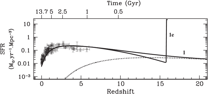
Figure 1.— The star formation rate for Model 1, and the rapid burst Model 1e. The dotted curve shows the SFR of the massive mode of Model 1. Data come from Hopkins (2004).

We do not here consider models with very massive stars in Pop III. In Daigne et al. (2006), two very massive mode models were considered in addition to Model 1 described above. In Model 2a, the massive mode consists of stars with masses in the range 140-260 M_⊙, and in Model 2b, the range used was 270-500 M_⊙. In Model 2b, there is significant metal enrichment (Heger & Woosley, 2002) which results in a diminished SFR and hence fewer cosmic rays available for ⁶Li production. In Model 2b, one expects total collapse and little or no production of cosmic rays.

The rate of core collapse supernovae (SNR) can be calculated directly in terms of the IMF and SFR

$$SNR=\int_{max(8M_{\odot},m_{min(t)})}^{m_{sup}}dm\phi(m)\psi(t-\tau(m)),$$ (6)

where $m_{min(t)}$ is the minimum mass of a star with lifetime, $\tau$, less than $t$. When a star undergoes core collapse, the mass of the remnant is determined by the mass of the progenitor. We assume that all stars of mass $m\gtrsim 8$ M_⊙ will die as supernovae. For stars of mass 8 M${}_{\odot}<m<30$ M_⊙, the remnant after core collapse will be a neutron star of $m\approx 1.5$ M_⊙. Stars with 30 M${}_{\odot}<m<100$ M_⊙ become black holes with mass approximately that of the star’s helium core before collapse (Heger et al., 2003). We take the mass of the Helium core to be

$$M_{He}=\frac{13}{24}\cdot(m-20\,M_{\odot})$$ (7)

for a star with main sequence mass $m$ (Heger & Woosley, 2002). The supernova rate ultimately determines the metal enrichment of the ISM and when coupled with the model of outflow also determines the metal enrichment of the IGM.

The energy emitted in each core collapse, $E_{cc}$ corresponds to the change in gravitational energy, 99% of which is emitted as neutrinos. In the cases where collapse results in a neutron star, $E_{cc}=3\times 10^{53}\,$ergs. For stars that collapse to black holes, $E_{cc}$ is proportional to the mass of the black hole. For masses less than 100 M_⊙, we take $E_{cc}=0.3M_{He}$ . We will parametrize the energy injected in cosmic rays per supernova as

$${\cal E}_{\rm CR}(m)={\epsilon E_{cc}(m)\over 100}\,,$$ (8)

where $\epsilon$ is the fraction of energy in the remaining 1% (i.e. energy not in neutrinos) deposited into cosmic rays. Given the IMF described above, the massive mode is dominated by 40 M_⊙ stars for which the total energy per SN in CRs is ${\cal E}_{III}=10^{52.8}\epsilon_{III}$ ergs. In contrast, the normal mode associated with Pop II, is dominated by lower mass stars for which the energy per SN in CRs is ${\cal E}_{II}=10^{51.5}\epsilon_{II}$ ergs. While it is quite plausible that $\epsilon_{II}$ and $\epsilon_{III}$ differ (indeed we would expect $\epsilon_{II}<\epsilon_{III}$), we will for simplicity assume $\epsilon_{II}=\epsilon_{III}=\epsilon=0.01-0.30$ as a broad and conservative range.

The SNR derived from Eq. 6 is shown for both Models 1 and 1e in Fig. 2 (lower panel). In the upper panel of Fig. 2, we show the energy density in CRs injected per year. The CR production rate in Model 1e (shown by the dot-dashed curves) is similar to that Model 1 (shown by the solid curves) below a redshift of about 10, as would be expected from the SFRs shown in Fig. 1. Dashed lines show the rates of CRs generated by massive Pop III SNe alone, while dotted lines correspond to Pop II SNe ejection. The energy density in cosmic rays is dominated at large redshift by Pop III SNe due to the corresponding IMFs and mass range associated with the two modes and the dependence of $E_{cc}$ on the progenitor mass.

The metallicity evolution in both the IGM and the ISM has been derived by Daigne et al. (2006) and is shown in Fig. 3. For Model 1e, the metallicity in the ISM rises very quickly to [Fe/H] $\sim-2.5$, whereas in Model 1, the initial enrichment occurs rapidly only to [Fe/H] $\sim-4$. The IGM abundance are several thousand times smaller. Both models have the same metallicity as a function of redshift below $z\sim 15$ in the ISM.

Figure 2.— CR history predicted by Daigne et al. (2006). The SNR (lower panel) and energy density in cosmic rays (upper panel) are shown in the case of Model 1 for Pop III (dashed), Pop II (dotted) and all SN (solid) and in the case of the model 1e (dot-dashed).

\begin{picture}(12.0,4.0)\centerline{\hbox{\psfig{width=244.69386pt}}} \end{picture}

Figure 3.— Evolution of metallicity in ISM and IGM versus redshift in Model 1 (dashed curves) and in Model 1e (solid curves).

3. Production of Lithium in the IGM

In RVOI, we considered a single burst of CRs whose total energy was fixed in an ad hoc way so as to reproduce the observed ⁶Li abundance. We now relate the production of CRs to the detailed model of cosmic chemical evolution in which the SN history is completely determined by the SFR and IMF of the model and are constrained to reionize the IGM at a redshift $z\simeq 11$, match the observed SFR at $z<6$, as well as chemical abundances at $z<3$. As a consequence, the energy density in cosmic rays is determined by the model and we can derive the abundance of Lithium produced in the IGM as described below.

3.1. Formalism of Cosmological Cosmic Rays

3.1.1 Ejection of CCR into the IGM

The total kinetic energy given initially to CRs by SN is

$${\cal E}_{\rm SN}(z)\,=(1+z)^{3}\int_{max(8M_{\odot},m_{min(t)})}^{m_{sup}}dm\phi(m)\psi(t-\tau(m)){\cal E}_{\rm CR}(m).$$ (9)

where it is understood that the appropriate IMF is used for computing CR energy density due to Pop II or Pop III SN. For example, using Eq. 9 we can estimate from Fig. 1, the Pop III contribution to the CR energy density. In Model 1, if we take $\psi\simeq 0.02$ M_⊙ yr^-1 Mpc^-3 from $z=10-30$, and approximate $\phi$ by a delta function at $m=40$ M_⊙, we obtain ${\cal E}_{\rm SN}(10)\simeq 7.8\times 10^{-13}\epsilon$ ergs/cm³. Note that the result of the full calculation of Eq. 9 is a factor of about 5 larger than this, because the contributions of more massive stars (more massive than 40 M_⊙) can not be neglected. This corresponds to ${\cal E}_{\rm SN}\simeq 3.6\times 10^{-12}\epsilon$ ergs/cm³. For Model 1e, we see that the burst is very intense, with a SFR which reaches 20 M_⊙ yr^-1 Mpc^-3, though the duration is only about $3\times 10^{6}$ yr. In this case, we approximate that ${\cal E}_{\rm SN}(16)\simeq 1.6\times 10^{-11}\epsilon$ ergs/cm³. The full calculation yields ${\cal E}_{\rm SN}\simeq 2.5\times 10^{-11}\epsilon$ ergs/cm³.

3.1.2 Source Spectrum

We next briefly describe our treatment of cosmological cosmic rays, their transport and the mechanism for the production of ⁶Li, in the case of one burst of CRs at a given redshift $z_{o}$. Our formalism is directly derived from the work of Montmerle (1977), hereafter M77. We begin by defining the source function for our CR distribution. The source function $Q(E,z)$ is defined as a power law in momentum,

$$Q(E,z)\ =\ C(z_{o})\frac{(E+E_{0})}{\left(E(E+2\,E_{0})\right)^{(\gamma+1)/2}}\delta(z-z_{o})[\mbox{GeV${}^{-1}$}\mbox{cm${}^{-3}$}\mbox{s${}^{-1}$}]\,,$$ (10)

where $C(z)$ is fixed by our normalization of the source function to the total energy from both Pop II and Pop III SNe using

$${\cal E}_{\rm SN}(z)={\cal E}_{\rm SN,II}(z)+{\cal E}_{\rm SN,III}(z)=\int_{E_{\rm min}}^{E_{\rm max}}E\,Q(E,z)\,{\rm d}E\$$ (11)

We take $E_{\rm min}=0.01$ MeV and $E_{\rm max}=10^{6}$ GeV . We set $\gamma=3$ in this section.

The efficiency of the SN to eject CRs outside the structure and into the IGM depends on many different physical parameters. Roughly, low energy particles will lose all their energy inside the structure and in this section, we take a simplified approach where the CRs spectrum is simply cut at a given energy, $E_{\rm cut}$ and decreased by a constant factor $\epsilon_{\rm shock}$.

$$Q_{\rm IGM}(E)=\left\{\begin{array}[]{ll}0&{\rm if\ }E<E_{\rm cut}\\ \epsilon_{\rm shock}\ Q(E)&{\rm if\ }E\geq E_{\rm cut}\end{array}\right.$$ (12)

In Daigne et al. (2006), the efficiency of the baryon outflow rate coming from the structures is dependent on the redshift. It accounts for the increasing escape velocity of the structure as the galaxy assembly is in progress. In fact, in Daigne et al. (2004) two sources of outflow were considered : a global outflow powered by stellar explosions (galactic winds) and an outflow corresponding to stellar supernova ejecta that are pushed directly out of the structures as chimneys. However, velocities in ISM gas are of the order of a few 100 km/s while CRs are mostly relativistic. Thus, the CR ejection processes considered here should be independent of the overall outflow of gas and heavy elements. As we will see, the production of Lithium is proportional to the energy available, and thus to $\epsilon_{\rm shock}$. Most of the CR production will occur at large redshift, when Pop III are dominant (especially in the case of the Model 1e). For simplicity, we will assume that all CRs are ejected from structures and adopt a constant value for $\epsilon_{\rm shock}=1$. We comment on the possibility of $\epsilon_{\rm shock}<1$ in §4.

3.1.3 Production of Lithium in the IGM

If $N_{i}(E,z)$ is the comoving number density per (GeV/n) of a given species at a given time or redshift, and energy, we define $N_{i,{\rm H}}(E,z)\,\equiv\,N(E,z)/n_{\rm H}(z)$, the abundance by number with respect to the ambient gaseous hydrogen (in units of (Gev/n)^-1). The evolution of $N_{i,{\rm H}}$ is defined through the transport function

$$\frac{\partial N_{i,{\rm H}}}{\partial t}+\frac{\partial}{\partial E}(bN_{i,{\rm H}})+\frac{N_{i,{\rm H}}}{T_{\rm D}}=Q_{i,{\rm H}}\,.$$ (13)

where ${T_{\rm D}}$ is the lifetime against destruction and $b$ describes the energy losses due to expansion or ionization processes ((Gev/n) s^-1). The energy and time dependencies can be separated as $b(E,z)=-B(E)f(z)$. We can distinguish two cases depending on whether losses are dominated by expansion or by ionization. The general form for the redshift dependence, when expansion dominates is $f_{\rm E}(z)=(1+z)^{-1}|{\rm d}z/{\rm d}t|\,H_{0}^{-1}$ (e.g. Wick, Dermer & Atoyan, 2004). Other contributions to $B$ or $f$, do not depend on the assumed cosmology and are given explicitly in M77.

In M77, two important quantities, $\mbox{$z^{\star}$}(E,E^{\prime},z)$ and $\mbox{$E_{s}^{{}^{\prime}}$}(E,z)$ are used in this formalism. Given a particle ($\alpha$ or lithium) with an energy $E$ at a redshift $z$, $\mbox{$z^{\star}$}(E,E^{\prime},z)$ corresponds to the redshift at which this particle had an energy $E^{\prime}$. $\mbox{$E_{s}^{{}^{\prime}}$}(E,z)$ is the initial energy required if this particle was produced at the redshift of the burst, $z_{s}$. In particular, $\mbox{$z^{\star}$}(E,\mbox{$E_{s}^{{}^{\prime}}$},z)=z_{s}$. The equation that defines $z^{\star}$ (Eq. A5, M77) is $\partial{\mbox{$z^{\star}$}}/\partial{E}=-\left[B(E)f(z)\,|{\rm d}z/{\rm d}t|\right]^{-1}\,\left(\partial{\mbox{$z^{\star}$}}/\partial{z}\right)$.

The evolution of the CCR $\alpha$ energy spectrum is derived, using Eq. A8 of M77

$$\Phi_{\alpha,{\rm H}}(E,z)={\phi_{\alpha}(E)\over\ n_{\rm H}^{0}}\frac{\beta}{\beta^{\prime}}\frac{\phi_{\alpha}(\mbox{$E_{s}^{{}^{\prime}}$})}{\phi_{\alpha}(E)}\left|\frac{{\rm d}z}{{\rm d}t}\right|_{z_{s}}\frac{\exp{(-\xi)}}{|b(E,z_{s})|}\,\frac{1}{\left|\partial\mbox{$z^{\star}$}/\partial E^{\prime}\right|_{{E_{s}^{\prime}}}}$$ (14)

where $\Phi_{\alpha,{\rm H}}(E,z)\equiv\Phi_{\alpha}(E,z)/n_{\rm H}(z)$ is the flux of $\alpha$’s per comoving volume

$$\Phi_{\alpha,{\rm H}}(E,z)=\beta\,N_{\alpha,{\rm H}}(E,z)$$ (15)

and $\beta$ ($\beta^{\prime}$) is the velocity corresponding to energy $E$ ($E_{s}^{{}^{\prime}}$); $\xi$ accounts for the destruction term (Eq. A9, M77). The CR injection spectrum, $\phi_{\alpha}$ is proportional to the source spectrum, $Q$.

The evolution of CR flux and the production of Lithium can be computed step by step directly with the transport function (Eq. 13).The abundance by number of lithium ($l$ = ⁶Li or ⁷Li) of energy $E$, produced at a given redshift $z$, is computed from

$${\partial N_{l,\,{\rm H}}(E,z)\over\partial t} = \int\sigma_{\alpha\alpha\rightarrow l}(E,E^{\prime})n_{\rm He}(z)\Phi_{\alpha\,,{\rm H}}(E^{\prime},z)\,{\rm d}E^{\prime}$$ (16)

$$= \sigma_{l}(E)K_{\alpha p}\Phi_{\alpha}(4\,E,z)\ \ [\mbox{(Gev/n)${}^{-1}$\,s${}^{-1}$}]\,,$$

where $\sigma_{\alpha\alpha\rightarrow l}(E,E^{\prime})=\sigma_{l}(E)\delta(E-E^{\prime}/4)$ and $K_{\alpha p}=0.08$ is the abundance by number of ⁴He/H. We use cross sections based on recent measurements related to the $\alpha+\alpha$ reaction and provide a new fit for the production of ⁶Li and ⁷Li (Mercer et al., 2001).

If we now consider the contribution of each individual burst at each redshift :

$$\begin{array}[]{lcl}{\rm(Li}/{\rm H)}(z)&=&{\rm Li}/{\rm H}_{\rm BBN}+\int_{z^{\prime}>z}{\rm d}z^{\prime}\int_{z}^{z^{\prime}}{\rm d}z^{\prime\prime}\\ &&\times\int_{E}\,\sigma_{l}(E)K_{\alpha p}{\Phi_{\alpha}}(4\,E,z^{\prime\prime})\,{\rm d}E\,|{\rm d}t/{\rm d}z^{\prime\prime}|\,|{\rm d}t/{\rm d}z^{\prime}|\,\,,\\ \end{array}$$

3.2. Results

Although the exact evolution of CR confinement is difficult to estimate, Ensslin (2003) discusses the relation of the diffusion coefficient with a magnetic field. Jubelgas et al. (2006) propose a simple model where this coefficient varies as the inverse of the square root of the density. The efficiency of the diffusion will then decrease with the density (as could be intuitively inferred). Then, at large redshift, the structures are smaller, less dense (e.g. Zhao et al., 2003) and the primordial magnetic field could be expected to confine less than it does today, which corresponds to a large value for $\epsilon_{\rm shock}$. As noted above, we will assume that $\epsilon_{\rm shock}=1$, bearing in mind that this approximation should not be valid at low redshifts ($z\lesssim 3$). In effect, our results for the production of Li will depend on the product of the CR escape efficiency, $\epsilon_{\rm shock}$, and the efficiency for converting SN energy into CRs, $\epsilon$. We will return to discuss the value of $\epsilon_{\rm shock}$ further below.

In this work, we have also introduced the energy cut-off parameter $E_{\rm cut}$. Its influence is actually straightforward. If $E_{\rm cut}$ is below 10 MeV, it does not modify our results for the Li abundance. Given the shape of the Li production cross section, only $\alpha$ particles around 10 MeV will produce Lithium. If particles have a lower energy initially, they will never be available to create Lithium. While if they are at higher energy, they will loose their energy during their transport through the medium, and at some time reach the optimum energy. Thus, if the cut-off is larger than 10 MeV, there will be a delay until some particles loose enough energy to produce Lithium efficiently. As shown in RVOI, the production of Li decreases very rapidly with time due to the global expansion, as a result this delay is unfavorable to Lithium production.

Pop III production of CRs dominate over Pop II at high redshift and most of the production of ⁶Li is due to the Pop III SN. Model 1e is closer to our RVOI assumption of a single burst. In Fig. 4, we show the evolution of the Li abundances for $\epsilon_{\rm shock}=1$ in Model 1 and Model 1e as labeled. The CR efficieny, $\epsilon$ has been fixed at $\epsilon=0.04$ so that in Model 1e, assuming that $E_{\rm cut}<10$ MeV, the total amount of Lithium produced at $z=3$ is [⁶Li] =-11.2. This value is perfectly consistent with the observations of ⁶Li in halo stars. In Model 1e, the sum of all energy within the burst of CRs at $z\sim 16$ corresponds to $10^{-12}$ ergs cm^-3 (for $\epsilon=0.04$), and according to RVOI ($6.3\times 10^{-13}$ at $z=10$) would result in producing ⁶Li at a value similar to that in the plateau.

In Model 1, the total energy, integrated over the full star formation history, is only about a factor of 3 less than that found in Model 1e. Consequently, the production of Lithium is reduced to $\epsilon(\mbox{${}^{6}$Li})=-11.7$ at $z=3$, for $\epsilon=0.04$ and thus is consistent with observations for an increased value of $\epsilon=0.15$. These values are consistent with expectations that roughly 10% of non-neutrino SN energy is converted to CR acceleration (Drury et al., 1989). For $\epsilon=0.15$, the energy density in cosmic rays in Model 1 is $5.4\times 10^{-13}$ ergs cm^-3 which is still slightly lower than the estimate in RVOI for a burst at $z=30$ and very similar to the one needed at $z=10$ to produce the ⁶Li plateau. Note that, as claimed in RVOI, ⁷Li is not overproduced by this process.

In Fig. 4, we also show the Pop III contribution alone to the Li production (dashed curves) for both Models 1 and 1e. As one can see, Li production is largely dominated by the Pop III contribution, though at lower redshifts, the production from the normal mode is non-negligible. If our calculation is extended to $z=0$, we obtain a small enhancement in the ⁶Li abundance as shown by the thin curves in Fig. 4. However, as noted earlier, below $z=3$, we expect that as the structures are larger and contain more baryons, CR escape will be limited resulting in a smaller value for $\epsilon_{\rm shock}$. In this case, we expect the in situ production of Li in the ISM to dominate as discussed below in §4.

For $E_{\rm cut}=100$ MeV, the production would be decreased by one order of magnitude. Had we chosen a spectral index $\gamma=2$, our results for both Models 1 and 1e would be diminished by a factor of about 40.

Figure 4.— The production of Lithium in the IGM by CCRs assuming $E_{\rm cut}<10$ MeV and $\epsilon_{\rm shock}=1$ as a function of redshift for both isotopes in both Models 1 and 1e. Here, $\epsilon$ is fixed at 0.04 so that Model 1e produces $\log$ ⁶Li/H = -11.2 at $z=3$. Since the Li abundance scales with $\epsilon$, adopting $\epsilon=0.15$, would increase the Model 1 abundance to -11.2 as well. The contribution from Pop III stars alone to the Li abundance is shown by the dashed curves.

The injection of CRs in the IGM will heat the medium. In fact, CCRs were predicted to heat the IGM and thus avoid the problem of overcooling in the IGM gas (Blanchard, Valls-Gabaud, & Mamon, 1992). Following the analysis of Samui, Subramanian, & Srianand (2005), we find that the temperature reaches as high as $10^{7}$ K in Model 1 at $z\sim 5$ when $E_{\rm cut}\lesssim 0.1$ MeV and $\epsilon_{\rm shock}=1.0$. There is a relatively strong correlation between the induced temperature and the CR energy cut-off as seen in Fig. 5 where the temperature due to CR heating is shown as a function of redshift for three choices of $E_{\rm cut}$. For $E_{\rm cut}=10$ MeV, we see that the temperature is held to the range $10^{4.5}-10^{5}$ K at $z=0$. Because we have fixed $\epsilon=0.04$ in Model 1e (as opposed to 0.15 in Model 1), we find somewhat lower temperatures for Model 1e as seen in Fig. 6. In addition, the lower temperature is partially due to the difference in the SN history: in Model 1e, there is a sudden heating of the IGM that can cool for a longer time than in Model 1 for which heating is more progressive. Observations of absorption lines in quasar spectra at $z\mbox{$\>\stackrel{{\scriptstyle<}}{{{}_{\sim}}}\>$}4$ set a conservative upper limit on the temperature of the IGM of $10^{5}$ K (e.g. Schaye et al., 2000; Rollinde, Petitjean, Pichon, 2001; Theuns et al., 2002). Thus both Models 1 and 1e, with $E_{\rm cut}=10$ MeV and $\epsilon_{\rm shock}=1.0$ will not overheat the IGM.

Figure 5.— The induced temperature by CCR heating in the IGM for Model 1 for three choices of the CR cut-off energy, $E_{\rm cut}$ as indicated.

Figure 6.— As in Fig. 5 for Model 1e.

The IGM temperatures shown in Fig. 5 and Fig. 6 should be viewed as an upper limit to the temperature in the IGM produced by CR heating. Firstly, to produce Fig. 5 and Fig. 6, we assumed $\epsilon_{\rm shock}=1.0$ at all times, including $z<3$. At low redshift, the Press-Schechter formalism breaks down as structures are no longer representative objects. As larger galaxies form, the ability to eject CRs diminishes and we expect $\epsilon_{\rm shock}$ to decrease. For $\epsilon_{\rm shock}=0$ below $z=3$, the temperatures would be lower by a factor of about 2 at $z=0$.

Secondly, our computation assumes that CRs propagate into the IGM in a homogeneous way. This is certainly not the case, as we expect the cosmic ray density and heating to be confined to the warm-hot IGM (WHIM). Correspondingly, the production of ⁶Li in the IGM may also occur in the WHIM embedding the structures. In fact, the temperatures shown in Fig. 5 are quite representative of the temperatures found in the WHIM (Cen & Ostriker, 1999; Simcoe et al., 2002). The heating of cluster gas by CRs used to produce ⁶Li was considered in Nath et al. (2006).

3.3. Discussion

A key question pertains to the propagation of CRs into the IGM and the degree to which the Lithium produced is accreted onto the Galaxy. We assumed that all CRs with energies above $E_{\rm cut}$ escape the structures and proto-clusters. Hence we have a homogeneous flux of cosmic rays in the IGM. More likely, in an inhomogeneous model, our flux would be contained in the WHIM. This scenario allows the Lithium produced to be accreted later, during the formation of the Galaxy. It then provides a prompt initial enrichment (PIE) at $z\sim 3$ required to explain the observed abundances. We can add this PIE to the standard GCR production of Lithium as in RVOI. In Fig. 7, we show the resulting evolution of ⁶Li as a function of [Fe/H]. The upper curve (solid blue) corresponds to Model 1 with $\epsilon=0.15$ and does an excellent job of fitting the observed ⁶Li abundances at low metallicity. The corresponding curve for Model 1e is nearly identical when $\epsilon$ is taken to be 0.04. A standard GCR model of ⁶Li production without a Population III enrichment is shown in Fig. 7 for comparison.

Figure 7.— The evolution of ⁶Li/H vs. [Fe/H] for standard galactic cosmic rays alone (shown by the solid green curve) and the addition of a PIE by the production of Lithium in the IGM as in Model 1 (shown by the solid blue curve) with $\epsilon=0.15$. Model 1e would yield a nearly identical result with $\epsilon=0.04$. ⁶Li data come from Asplund et al. (2006) with the exception of the lowest metallicity star which comes from Inoue et al. (2005).

As in RVOI, we require some depletion of ⁶Li at higher metallicities. This should not be particularly surprising since all models GCRN predict a linear growth of [⁶Li] versus [Fe/H]. In standard GCRN, the ⁶Li abundance matched the observations only for [Fe/H] $\simeq-2$. This fact was often associated with an energetics problem concerning the production of ⁶Li (Ramaty et al., 1997, 2000; Fields et al., 2001). Pop III production of ⁶Li can successfully account for the ⁶Li plateau at low metallicity and together with GCR production accounts for the present-day meteoritic value. As a result, we have overproduced ⁶Li at [Fe/H] $\sim-1$. This could be accounted for by depletion which is expected to be important at higher metallicities. It is also plausible that the degree of depletion increases with increasing metallicity (Piau, 2005).

The large temperatures produced in the IGM, prohibit the homogenous production of ⁶Li (if $E_{\rm cut}<10$ MeV). If one considers that the ⁶Li production processes occur in the WHIM, the constraint on the temperature are very much relaxed. Indeed, this medium is denser, located around the galaxies or in filaments of clusters of galaxies. Hydrodynamic simulations (e.g. Cen & Ostriker, 1999; Davé et al., 2001; Kang et al., 2005) have long since shown that the WHIM, heated by shock waves during structure formation, displays two different phases: a cold phase, at T$\mbox{$\>\stackrel{{\scriptstyle<}}{{{}_{\sim}}}\>$}\ 10^{5}$ K and a hot phase, at T$\sim\ 10^{5-7}$K. The cold one is observed through the O vi absorption lines whose width distribution constrains the temperature (e.g. Bergeron et al., 2002). The hot one may be responsible for the soft X-ray background, observed by Chandra (e.g. Nicastro et al., 2003; Mc Kernan et al., 2003) and its temperature can be constrained by the observation of broad H I lines (e.g. with FUSE, Richter et al., 2004) or of O vii lines with Chandra (Fang et al., 2002) and, in the future, with XEUS (e.g. Viel et al., 2003). Consequently, the temperatures derived in our scenario, when taken in the context of the WHIM, are acceptable. In addition, in a dense region, other processes, such as H2 line cooling, could lower the temperature even more. Note that in Soltan (2006) hydrodynamical simulations indicate that a substantial fraction of baryons in the universe remains in a diffuse component WHIM. This component is predicted to be at T$\sim\ 10^{5-7}$K, as noted previously.

Finally, one should bare in mind that we set $\epsilon_{\rm shock}$ equal to a constant value (1.0). The exact value of $\epsilon_{\rm shock}$ depends on the strength of the magnetic field at each epoch, on the density of the ISM etc… It is difficult to accurately estimate the escape fraction, which is certainly dependent on the energy of the particles (roughly modeled here by $E_{\rm cut}$). Ensslin et al. (2006) have begun an investigation into the propagation of CRs in the ISM taking into account all physical components. To date, they are only able to obtain the mean values of the physical parameters, but this is certainly a path to follow. Note that if the efficiency is much less than one, the induced IGM temperature is reduced, as is the initial enrichment of ⁶Li. This will be partially offset because the density in the WHIM is larger than the mean density of the universe (used in the above formalism), and it is quite plausible that CRs are trapped there and increase the initial enrichment of Lithium.

4. Production of Lithium in the ISM

The model discussed in the previous section was a homogeneous model in which the IGM flux of CCRs was controlled by the SN history and in particular, our choices of $\epsilon_{II}$, $\epsilon_{III}$ and as discussed above, $\epsilon_{\rm shock}$. If CR propagation into the WHIM is efficient, i.e. $\epsilon_{\rm shock}=1$, their interaction with the medium will produce the required amount of Lithium as a PIE, as discussed in the previous section.

In fact, we expect CR propagation to be limited by diffusion, particularly at lower redshift so that they are concentrated in or near the structures leading to not only enhanced ⁶Li production but also heating of the eventual intra-cluster medium as well as the warm-hot IGM. In this section, we will outline the computation of ⁶Li production in the structures of the hierarchical formation scenario that end with our Galaxy. We assume that the CR energy output of SN is constant over a sufficiently long time so that we can work in the context of a leaky box model. We can then adopt the physical formalism developed for LiBeB production in our Galaxy (Meneguzzi, Audouze & Reeves, 1971), hereafter MAR, (Vangioni-Flam et al., 2000; Fields, Olive, & Schramm, 1994).

In GCRN, it is common to normalize the flux of CRs by reproducing the observed abundance of Beryllium at present. In contrast, here, we rely on the same cosmological models described above when we consider the cosmological evolution of CR and the ⁶Li abundance. In addition, we must take into account the evolution with redshift of several physical parameters defined below.

Finally, the production of Lithium in the IGM as described in the previous section acted as an effective prompt initial enrichment of ⁶Li in the IGM which by subsequent accretion and growth of structure led to the ⁶Li plateau observed in our Galaxy. In the case of ISM production, each structure along the hierarchical tree inherits the medium as modified by SN that explode in the past. This explains the relation between metallicity and redshift seen in Fig. 3. Thus, when we observe Lithium in a star at a given metallicity, we must use the Lithium abundance present when this same metallicity was reached.

4.1. Formalism

As before we compute the total rate of energy density put into CRs from SN, ${\cal E}_{\rm SN}$, using Eq. 9. We use the same source term, $Q(E,z)$, defined in Eq. 10. In the framework of a diffusion model in a medium of density $\rho$, it is useful to consider the scaled source $q=Q/\rho$. The normalization of $Q$ is related to the energy density inside the structures. However, ${\cal E}_{\rm SN}$ corresponds to the energy density provided by SN if it was uniformly distributed within the universe, which was true when considering the diffusion into the IGM previously. Since this energy is now confined within the structure, the density there must be larger by a factor $\rho/f_{b}\rho_{b}$, where $\rho_{b}$ is the average baryon energy density in the Universe and $f_{b}$ is the fraction of baryons found in structures. Therefore source function is normalized using

$$\int E\,q(E,z)\,{\rm d}E\ =\ \frac{{\cal E_{\rm SN}}(z)}{f_{b}(z)\,\rho_{c}\,\Omega_{b}}.$$ (17)

Note that all parameters that vary with redshift are given with the hierarchical model provided by Daigne et al. (2006).

By interaction with the particles present inside the medium, CR particles lose their energy. The rate of energy lost is noted $b$. We update the relations in MAR using Mannheim & Schickeiser (1994). Note that this rate depends on the ionization fraction of the medium, $x_{e}$. We use here $x_{e}=0.01$ but we checked that one could go up to $x_{e}=0.1$ without modifying our results. It is also convenient to define the quantity $w=b/\rho v$ where $v$ is the velocity of the CR particle. Because of the physical properties of the medium and the presence of a magnetic field, CRs will be confined to some characteristic escape length, $\Lambda$ which in GCRN may range from 10 - 1000 gcm^-2. Under these condition, the solution of the diffusion equation (MAR) for the flux $\Phi_{\alpha}$ is

$$\begin{array}[]{lcl}\Phi_{\alpha}(E,z)&=&\frac{1}{w}\int{\rm d}E^{\prime}q_{\alpha}(E,z)\exp{\left(-\frac{R(E^{\prime})-R(E)}{\Lambda(z)}\right)}\\ &=&\frac{{\cal E_{\rm SN}}(z)}{f_{b}(z)\,\rho_{c}\,\Omega_{b}}\,\mbox{${\rm K}_{\alpha{\rm p}}$}\,g(\Lambda,x_{e},\gamma,z)\end{array}$$ (18)

The term $q_{\alpha}=\mbox{${\rm K}_{\alpha{\rm p}}$}\,q$ (evaluated appropriately in the ISM) is the source of $\alpha$ particles; and $R(E)=\int_{0}^{E}{\rm d}E/w$ is the ionization range which characterizes the average amount of material that an $\alpha$ particle with energy $E$ can travel before ionization losses will stop it. $g$ is a function that corresponds to the diffusion solution.

The rate of Lithium production of Lithium is then

$$\begin{array}[]{lcl}\frac{{\rm d}missing}{{\rm d}t}(\frac{\rm Li}{\rm H})(z)&=&\left[\frac{\alpha}{\rm H}\right]\int\sigma\,\Phi_{\alpha}(E,z)\,{\rm d}E\\ &=&\left[\frac{\alpha}{\rm H}\right]K_{\alpha p}\frac{{\cal E_{\rm SN}}(z)}{f_{b}(z)\,\rho_{c}\,\Omega_{b}}f(\Lambda,x_{e},\gamma,z)\end{array}$$ (19)

Thus, if the physical properties of the structures ($\Lambda,x_{e}$) as well as those of the SN ejection processes ($\gamma$) do not evolve with time,

$$\left(\frac{\rm Li}{\rm H}\right)(z)=K_{\alpha p}f(\Lambda,x_{e},\gamma)\int_{z}^{\infty}\frac{{\cal E_{\rm SN}}(z)}{f_{b}(z)\,\rho_{c}\,\Omega_{b}}\frac{{\rm d}t}{{\rm d}z}{\rm d}z$$ (20)

The result of the integral is shown in Fig. 8 for both models considered here.

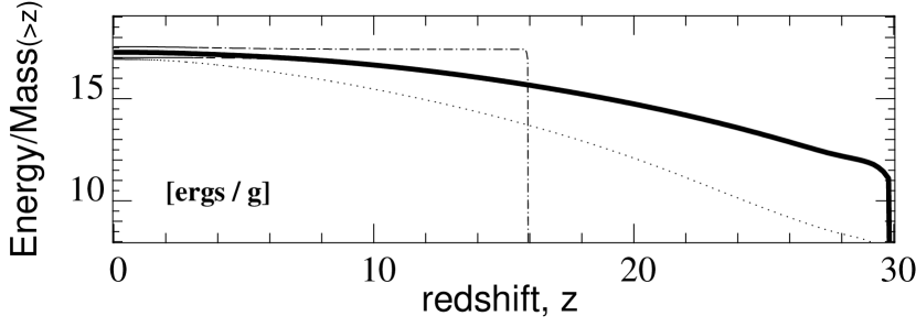
Figure 8.— The cumulative ratio of the energy deposited in CRs to the mass of the structure as determined by the integral in Eq. 20 (curves are as in Fig. 2).

4.2. Discussion

The main parameters of this scenario are $\Lambda$ and $\gamma$. $\Lambda$ is likely to be typically 10 gcm^-2 in our Galaxy. At larger redshift, as discussed in §3.2, $\Lambda$ is expected to be smaller due to the evolution of both the density of the structure and of the amplitude of the magnetic field. A lower value of $\Lambda$ implies that CRs escape faster out of the structure, and thus produce less Lithium. This can be seen directly in Eq. 18. Indeed, one expects a strong correlation between $\Lambda$ and the parameter $\epsilon_{\rm shock}$ discussed earlier with very small values of $\Lambda$ corresponding to values of $\epsilon_{\rm shock}\approx 1$.

The evolution of the abundance of ⁶Li can computed directly as a function of metallicity (see above). As discussed earlier, this scenario, based on the Press-Schechter formalism will likely break down at low redshift. If one follows the production of ⁶Li up to that point $z\approx 3$, one can in fact place a limit to $\Lambda$ to avoid the over-production of ⁶Li in structures. In Model 1, we find that $\Lambda\leq 10^{-5}$ g cm^-2. The upper limit in Model 1e is a factor of 4 times larger. These values are so low that our choice of $\epsilon_{\rm shock}=1$ appears to have been well justified. Subsequently, we expect $\Lambda$ to increase as the structure evolves into a galaxy where standard GCR becomes important.

5. Summary

The observation of a ⁶Li plateau in halo stars at low metallicity poses a challenge to standard models of ⁶Li production via Galactic cosmic ray nucleosynthesis. The level of the plateau is about 1000 times larger than the standard big bang nucleosynthesis value and about a factor of 10 larger than the GCRN value at [Fe/H] = -3.

In RVOI, we showed that an early burst of cosmic rays injected into the IGM would produce a prompt initial enrichment of ⁶Li. There, we used the observed plateau value to normalize the energy density of CRs. Here we applied this mechanism to a detailed model of cosmic chemical evolution. The model was designed to reproduce the observed star formation rate at redshift $z\lesssim 6$, the observed chemical abundances in damped Lyman alpha absorbers and in the intergalactic medium, and to allow for an early reionization of the Universe at $z\sim 11$ as indicated by the third year results released by WMAP. As a consequence, Daigne et al. (2006), was able to compute the supernova rate as a function of redshift. This SNR was employed here to compute the resulting energy density in cosmic rays.

Our results depend on the efficiency to which cosmic rays are accelerated out of the first star forming structures. We found that for efficiencies, $\epsilon_{\rm shock}=1$, the Models 1 and 1e discussed in Daigne et al. (2006) can produce a plateau in ⁶Li at the right abundance level at low redshift when the SN energy deposited in CRs is about 4-15% of the available kinetic energy. This conforms well with models of CR acceleration (Drury et al., 1989). As in standard GCRN, ⁶Li depletion at higher metallicities is necessary if the plateau is found to persist. By computing the CR heating of the IGM, we conclude that most of the CR propagation and hence ⁶Li production should be confined to the warm-hot IGM.

We also compute the in situ production of ⁶Li in star forming structures. Indeed, unless CRs are allowed to escape, that is, unless the characteristic escape length is significantly smaller than 10 g/cm² at high redshift the ⁶Li abundance would greatly exceed the observed value.

Clearly a definitive result for the production of ⁶Li at high redshift or at low metallicity will require a more detailed model for the ejection and propagation of CRs in the early structure forming Universe. The mechanisms described here would certainly produce a plateau at low metallicity. The absolute abundance level is uncertain but can be tied to a set of reasonable chosen physical parameters.

References

- Asplund et al. (2006) Asplund, M. et al. , 2006, astro ph 0510630,ApJ, in press
- Bergeron et al. (2002) Bergeron, J., Aracil, B., Petitjean, P. & Pichon, C. 2002, A&A, 396, L11
- Blanchard, Valls-Gabaud, & Mamon (1992) Blanchard, A., Valls-Gabaud, D., & Mamon, G.A. 1992, A&A, 264, 365
- Cayrel et al. (1999) Cayrel, R., Spite M., Spite F., Vangioni-Flam, E., Cassé, M. and Audouze, J. 1999, A&A, 343, 923
- Cen & Ostriker (1999) Cen, R. & Ostriker, J.P. 1999, ApJ, 514, 1
- Coc et al. (2004) Coc, A., Vangioni-Flam, E., Descouvemont, P., Adahchour, A., & Angulo, C. 2004, ApJ, 600, 544
- Cuoco et al. (2004) Cuoco, A., Iocco, I., Mangano, G., Pisanti, O., & Serpico, P.D. 2004, Int Mod Phys, A19, 4431
- Cyburt, Fields, & Olive (2001) Cyburt, R.H., Fields, B.D., & Olive, K.A. 2001, New Astronomy, 6, 215
- Cyburt, Fields, & Olive (2003) Cyburt, R.H., Fields, B.D., & Olive, K.A. 2003, Phys. Lett., B567, 227
- Cyburt (2004) Cyburt, R., 2004, Phys. Rev., D, 70, 023505
- Daigne et al. (2004) Daigne, F., Olive, K. A., Vangioni-Flam, E., Silk, J., & Audouze, J. 2004, ApJ, 617, 693
- Daigne et al. (2006) Daigne, F., Olive, K. A., Silk, J., Stoehr, F., & Vangioni-Flam, E. 2006 ,astro-ph/0509183, ApJ in press
- Davé et al. (2001) Davé, R. et al. 2001, ApJ, 552, 473
- Drury et al. (1989) Drury, L. O., Markiewicz, W. J., & Voelk, H. J. 1989, A&A, 225, 179
- Ensslin (2003) Ensslin, T.A. 2003, A&A, 399, 409
- Ensslin et al. (2006) Ensslin, T.A., Pfrommer, C., Springel, V. & jubelgas, M. 2006, astro-ph/0603484
- Fang et al. (2002) Fang, T., Marshall, H. L., Lee, J. C., Davis, D. S. & Canizares, C. R. 2002, ApJ, 572, 127
- Fields & Olive (1999) Fields, B.D., & Olive, K.A., 1999, New. Astron. 4, 255
- Fields, Olive, & Schramm (1994) Fields, B.D., Olive, K.A., & Schramm, D.N. 1994, ApJ, 435, 185
- Fields et al. (2001) Fields, B. D., Olive, K. A., Cassé, M., & Vangioni-Flam, E. 2001, A&A, 370, 623
- Fields & Prodanović (2005) Fields, B. D., & Prodanović, T. 2005, ApJ, 623, 877
- Heger et al. (2003) Heger, A., Fryer, C.L., Woosley, S.E., Langer, N., & Hartmann, D.H. 2003, ApJ, 591, 288
- Heger & Woosley (2002) Heger, A. & Woosley, S. E. 2002, ApJ, 567, 532
- Hobbs & Thorburn (1994) Hobbs, L.M. & Thorburn, J.A. 1994, ApJ, 428, L25
- Hobbs & Thorburn (1997) Hobbs, L.M. & Thorburn, J.A. 1997, ApJ, 491, 772
- Hopkins (2004) Hopkins, A.M., 2004, ApJ, 615, 209.
- Inoue et al. (2005) Inoue, S., 2005, IAU Symposium 228, Edts V. Hill, P. Francois, F. Primas, Cambridge Un. Press, p. 59.
- Jedamzik (2000) Jedamzik, K. 2000, Phys. Rev. Lett., 84, L15
- Jedamzik (2004a) Jedamzik, K. 2004a, Phys. Rev. D, 70, 063524
- Jedamzik (2004b) Jedamzik, K. 2004b, Phys. Rev. D, 70, 083510
- Jedamzik et al. (2005) Jedamzik, K., Choi, K. Y., Roszkowski, L., & Ruiz de Austri, R. 2005, hep-ph/0512044
- Jenkins et al. (2001) Jenkins, A., et al. 2001, MNRAS, 321, 372
- Jubelgas et al. (2006) Jubelgas, M., Springel, V., Ensslin, T. & Pfrommer, C. 2006, astro-ph/0603485
- Kang et al. (2005) Kang, H., Ruy, D., Cen, R. & Song, D. 2005, ApJ, 620, 21
- Kawasaki et al. (2005) Kawasaki, M., Kohri, K., & Moroi, T. 2005, Phys. Rev. D, 71, 083502
- Kusakabe, Kajino & Mathews (2006) Kusakabe, M., Kajino, T., & Mathews, G.J. 2006, astro-ph/0605255
- Mannheim & Schickeiser (1994) Mannheim, K. & Schickeiser, R. 1994, A&A, 286, 983
- Mc Kernan et al. (2003) Mc Kernan, B., Yaqoob, T, Mushotzky, R., George, I.M. & Turner, T.J. 2003, ApJ, 598, L83
- Meléndez & Ramírez (2004) Meléndez, J. & Ramírez, I. 2004, ApJ, 615, 33
- Meneguzzi, Audouze & Reeves (1971) Meneguzzi, M., Audouze, J. & Reeves, H. 1971, A&A, 15, 337
- Mercer et al. (2001) Mercer, D.J., Austin, S. M., Brown, J. A., Danczyk, S. A., Hirzebruch, S. E., Kelley, J. H., Suomijärvi, T., Roberts, D. A., & Walker, T. P. 2001, Phys. Rev. C, 63, 065805
- Montmerle (1977) Montmerle, T. 1977a, ApJ, 216, 177 (M77)
- Nath et al. (2006) Nath, B. B., Madau, P., & Silk, J. 2006, MNRAS, 366, L35
- Nicastro et al. (2003) Nicastro, F. et al. 2003, Nature, 421, 719
- Nissen et al. (2000) Nissen, P.E., Asplund, M., Hill, V. & D’Odorico, S. 2000, A & A 357, L49
- Piau (2005) Piau, L. 2005, astro-ph/0511402
- Pospelov (2006) Pospelov, M. 2006, astro-ph/0605215
- Press & Schechter (1974) Press, W. H. & Schechter, P. 1974, ApJ, 187, 425
- Ramaty et al. (1997) Ramaty, R., Kozlovsky, B., Lingenfelter, R. E., & Reeves, H. 1997, ApJ, 488, 730
- Ramaty et al. (2000) Ramaty, R., Scully, S. T., Lingenfelter, R. E., & Kozlovsky, B. 2000, ApJ, 534, 747
- Richter et al. (2004) Richter, P., Savage, B.D., Tripp, T.M. & Sembach, K.R. 2004, ApJSS, 153,165
- Rollinde, Petitjean, Pichon (2001) Rollinde, E., Petitjean, P. & Pichon, C. 2001, A&A, 376, 28
- Rollinde, Vangioni, & Olive (2005) Rollinde, E., Vangioni, E., & Olive, K. 2005, ApJ, 627, 666
- Ryan et al. (2000) Ryan, S.G., Beers, T.C., Olive, K.A., Fields, B.D., & Norris, J.E. 2000, ApJL, 530, L57
- Samui, Subramanian, & Srianand (2005) Samui, S., Subramanian, K. & Srianand, R. 2005, astro-ph/0505590
- Schaye et al. (2000) Schaye, J., Theuns, T., Rauch, M., Efstathiou, G., & Sargent, W. L. W. 2000, MNRAS, 318, 817
- Simcoe et al. (2002) Simcoe, R. A., Sargent, W. L. W., & Rauch, M. 2002, ApJ, 578, 737
- Smith, Lambert, & Nissen (1993) Smith, V.V., Lambert D.L. & Nissen P.E. 1993, ApJ, 408, 262
- Smith, Lambert, & Nissen (1998) Smith, V.V., Lambert, D.L. & Nissen, P.E., 1998, ApJ, 506, 405
- Soltan (2006) Soltan, A.M., 2006 astroph 0604465
- Spergel et al. (2003) Spergel, D. N., et al. 2003, ApJS, 148, 175
- Spergel et al. (2006) Spergel, D. N., et al. 2006, astro-ph 0603449
- Spite & Spite (1982) Spite, F. & Spite, M. 1982. A&A, 115, 357
- Steigman et al. (1993) Steigman, G., Fields, B.D., Olive, K.A., Schramm, D.N., & Walker, T.P. 1993, ApJ, 415, L35
- Suzuki & Inoue (2002) Suzuki, T.K., & Inoue, S. 2002, ApJ, 573,168
- Theuns et al. (2002) Theuns, T., Bernardi, M., Frieman, J., Hewett, P., Schaye, J., Sheth, R. K. & Subbarao, M. 2002, ApJ, 574, 111
- Thomas, Schramm, Olive, & Fields (1993) Thomas, D., Schramm, D. N., Olive, K. A., & Fields, B. D. 1993, ApJ, 406, 569
- Vangioni-Flam et al. (1999) Vangioni-Flam, E. et al. , 1999, New. Astron. 4, 245
- Vangioni-Flam et al. (2000) Vangioni-Flam, E., Cassé, M. and Audouze, J. 2000, Phys.Rep, 333-334, 365
- Viel et al. (2003) Viel, M., Branchini, E., Cen, R., Matarrese, S., Mazzotta, P. & Ostriker, J. P. 2003, MNRAS, 341, 792
- Wick, Dermer & Atoyan (2004) Wick, S. D., Dermer, C. D., & Atoyan, A. 2004, AstroParticles Physics, 21, 125
- Zhao et al. (2003) Zhao, D.H., Mo, H.J., Jing, Y.P., & Börner, G. 2003, MNRAS, 339, 12