We discuss the Buchert equations, which describe the average expansion of an inhomogeneous dust universe. In the limit of small perturbations, they reduce to the Friedmann-Robertson-Walker equations. However, when the universe is very inhomogeneous, the behaviour can be qualitatively different from the FRW case. In particular, the average expansion rate can accelerate even though the local expansion rate decelerates everywhere. We clarify the physical meaning of this paradoxical feature with a simple toy model, and demonstrate how acceleration is intimately connected with gravitational collapse. This provides a link to structure formation, which in turn has a preferred time around the era when acceleration has been observed to start.

This essay was awarded honorable mention in the
2006 Gravity Research Foundation essay competition.

The coincidence problem.

Perhaps the most surprising discovery in modern cosmology is that the expansion of the universe has apparently accelerated in the recent past. The observations have usually been interpreted in the context of the homogeneous and isotropic Friedmann-Robertson-Walker (FRW) model. The Einstein equation then reduces to the FRW equations:

$$3\frac{\ddot{a}}{a} = -4\pi G_{N}(\rho+3p)$$ (1)

$$3\frac{\dot{a}^{2}}{a^{2}} = 8\pi G_{N}\rho-3\frac{k}{a^{2}}$$ (3)

$$\dot{\rho}+3\frac{\dot{a}}{a}(\rho+p)=0\ ,$$

where $G_{N}$ is Newton’s constant, dot denotes derivative with respect to the proper time $t$ of comoving observers, $a(t)$ is the scale factor of the universe, $\rho(t)$ and $p(t)$ are the energy density and pressure, respectively, and $k=0,+1,-1$ gives the spatial curvature of the hypersurfaces of constant $t$.

According to (1), the expansion of a universe which contains only ordinary matter with non-negative energy density and pressure decelerates, as expected on the grounds that gravity is attractive. The observations can then be explained only with repulsive gravity, either by introducing matter with negative pressure or by modifying the theory of gravity. Such models suffer from the coincidence problem: they do not explain why the acceleration has started in the recent past. If there is a dynamical explanation, it is presumably related to the dynamics we see in the universe. The most significant change at late times is the formation of large scale structure, so it seems a natural possibility that the observed deviation from the prediction of deceleration in the homogeneous and isotropic matter-dominated model would be related to the growth of inhomogeneities.

The fitting problem.

The rationale for the FRW model is that the universe appears to be homogeneous and isotropic when averaged over large scales. According to this reasoning, one first takes the average of the metric and the energy-momentum tensor, and then plugs these smooth quantities into the Einstein equation. However, physically one should first plug the inhomogeneous quantities into the Einstein equation and then take the average. Because the Einstein equation is non-linear, these two procedures are not equivalent. This leads to the fitting problem discussed by George Ellis in 1983 [1]: how does one find the average model which best fits the real inhomogeneous universe? The difference between the behaviour of the average and smooth quantities is also known as backreaction [2].

The Buchert equations.

Let us look at backreaction in a universe which contains only zero pressure dust. Assuming that the dust is irrotational, but allowing for otherwise arbitrary inhomogeneity, the Einstein equation yields the following exact local equations [3]:

$$\dot{\theta}+\frac{1}{3}\theta^{2} = -4\pi G_{N}\rho-2\sigma^{2}$$ (4)

$$\frac{1}{3}\theta^{2} = 8\pi G_{N}\rho-\frac{1}{2}\mathcal{R}+\sigma^{2}$$ (6)

$$\dot{\rho}+\theta\rho=0\ ,$$

where $\theta(t,\bi{x})$ is the expansion rate of the local volume element, $\rho(t,\bi{x})\geq 0$ is the energy density, $\sigma^{2}(t,\bi{x})\geq 0$ is the shear and $\mathcal{R}(t,\bi{x})$ is the spatial curvature. At first sight it might seem that acceleration is ruled out just as in the FRW case: according to (4), the expansion decelerates at every point in space. However, let us look more closely. Averaging (4)–(6) over the hypersurface of constant $t$, with volume measure $\sqrt{{}^{(3)}g}$ and volume $V(t)=\int d^{3}x\sqrt{{}^{(3)}g}$, we obtain the exact Buchert equations [3]:

$$3\frac{\ddot{a}}{a} = -4\pi G_{N}\langle{\rho}\rangle+\mathcal{Q}$$ (7)

$$3\frac{\dot{a}^{2}}{a^{2}} = 8\pi G_{N}\langle{\rho}\rangle-\frac{1}{2}\langle{\mathcal{R}}\rangle-\frac{1}{2}\mathcal{Q}$$ (9)

$$\partial_{t}\langle{\rho}\rangle+3\frac{\dot{a}}{a}\langle{\rho}\rangle=0$$

$$\mathcal{Q} \equiv \frac{2}{3}\left(\langle{\theta^{2}}\rangle-\langle{\theta}\rangle^{2}\right)-2\langle{\sigma^{2}}\rangle\ ,$$ (10)

where the scale factor $a$ is defined as $a(t)\propto V(t)^{1/3}$ and $\langle{A}\rangle\equiv\int d^{3}x\sqrt{{}^{(3)}g}\,A/\int d^{3}x\sqrt{{}^{(3)}g}$ is the spatial average of the quantity $A$.

The Buchert equations (7)–(10) are the generalisation of the FRW equations (1)–(3) for an inhomogeneous dust universe. The effect of the inhomogeneity is contained in the new term $\mathcal{Q}$. If the variance of the expansion rate and the shear are small, the Buchert equations reduce to the FRW equations. In fact, this is the way to derive the FRW equations (for dust) and quantify their domain of validity. The applicability of linear perturbation theory also follows straightforwardly, since $\mathcal{Q}$ is quadratic in small perturbations. Conversely, the Buchert equations show that when there are significant inhomogeneities, the FRW equations are not valid. In particular, the average acceleration (7) can be positive if the variance of the expansion rate is large.

It seems paradoxical that the average expansion can accelerate even though the local expansion decelerates everywhere. We will clarify the physical meaning of the average acceleration with a toy model, and find that the answer sounds as paradoxical as the question: the average expansion rate accelerates because there are regions which are collapsing.

Acceleration from collapse.

When the universe becomes matter-dominated, it is well described by the FRW equations plus linear, growing perturbations. Within an overdense patch, the expansion slows down relative to the mean and eventually the perturbation turns around, collapses and stabilises at a finite size. Underdense patches in turn expand faster than the mean and become nearly empty regions called voids. Part of the universe is always undergoing gravitational collapse, and part is always becoming emptier.

When a density perturbation becomes of order one, it passes outside the range of validity of the FRW equations plus linear perturbations. A simple non-linear model for structure formation is the collapse of a spherical overdensity. In this case the Buchert equations (7)–(10) reduce in the Newtonian limit to the spherical collapse model [4], according to which the overdense region behaves like an independent FRW universe with positive spatial curvature (see e.g. [5]). Likewise, an underdense region can be described as a FRW universe with negative spatial curvature.

What is true for the perturbations also applies to the mean: once there are large perturbations in a significant fraction of space, the average expansion no longer follows the FRW equations, opening the door for accelerating expansion.

Let us consider a toy model which consists of the union of an underdense region representing a void and an overdense region representing a collapsing structure. We denote the scale factors of the regions $a_{1},a_{2}$, where 1 refers to the underdense and 2 to the overdense region; the corresponding Hubble parameters are $H_{1}\equiv\dot{a}_{1}/a_{1}$, $H_{2}\equiv\dot{a}_{2}/a_{2}$. The overall scale factor is given by $a^{3}=a_{1}^{3}+a_{2}^{3}$, and the average Hubble and deceleration parameters are

$$\!\!\!\!\!\!\!\!\!\!\!\!\!\!H \equiv \frac{\dot{a}}{a}=\frac{a_{1}^{3}}{a_{1}^{3}+a_{2}^{3}}H_{1}+\frac{a_{2}^{3}}{a_{1}^{3}+a_{2}^{3}}H_{2}\equiv H_{1}\left(1-v+vh\right)$$ (11)

$$\!\!\!\!\!\!\!\!\!\!\!\!\!\!q \equiv -\frac{1}{H^{2}}\frac{\ddot{a}}{a}=q_{1}\frac{1-v}{(1-v+hv)^{2}}+q_{2}\frac{vh^{2}}{(1-v+hv)^{2}}-2\frac{v(1-v)(1-h)^{2}}{(1-v+hv)^{2}}\ ,$$ (12)

where $q_{1},q_{2}$ are the deceleration parameters of regions 1 and 2, $v\equiv a_{2}^{3}/(a_{1}^{3}+a_{2}^{3})$ is the fraction of volume in region 2, and $h\equiv H_{2}/H_{1}$ is the relative expansion rate.

The Hubble rate is simply the volume-weighed average of $H_{1}$ and $H_{2}$. This is not the case for the deceleration parameter $q$: there is a third term which is negative and contributes to acceleration, corresponding to the fact that $\mathcal{Q}$ in (7) is positive.

Let us for simplicity take the void region to be completely empty, so that $a_{1}\propto t$, $q_{1}=0$. For the overdense region we have $a_{2}\propto 1-\cos\theta$, where $\theta$ is the development angle determined by $t\propto\theta-\sin\theta$. This gives $q_{2}=(1-\cos\theta)/\sin^{2}\theta$. The overdense region expands from $\theta=0$, turns around at $\theta=\pi$ and is taken (by hand) to stabilise at $\theta=3\pi/2$. Denoting the volume fractions occupied by the regions at turnaround $f_{1}=1-f_{2}$, $f_{2}$, we have

$$\!\!\!\!\!\!\!\!\!\!\!v=\frac{f_{2}\pi^{3}(1-\cos\theta)^{3}}{8(1-f_{2})(\theta-\sin\theta)^{3}+f_{2}\pi^{3}(1-\cos\theta)^{3}}\quad,\quad h=\frac{\sin\theta(\theta-\sin\theta)}{(1-\cos\theta)^{2}}\ .$$ (13)

Inserting (13) into (12), it is straightforward to establish that the acceleration can be positive. Figure 1 shows the deceleration parameter $q$ for this toy model with $f_{2}=0.3$ and for the $\Lambda$CDM model with $\Omega_{\Lambda}=0.7$ at $\theta=3\pi/2$. The toy model is not to be taken seriously beyond qualitative features, but we see that it is possible for backreaction to produce acceleration not dissimilar to what is observed.

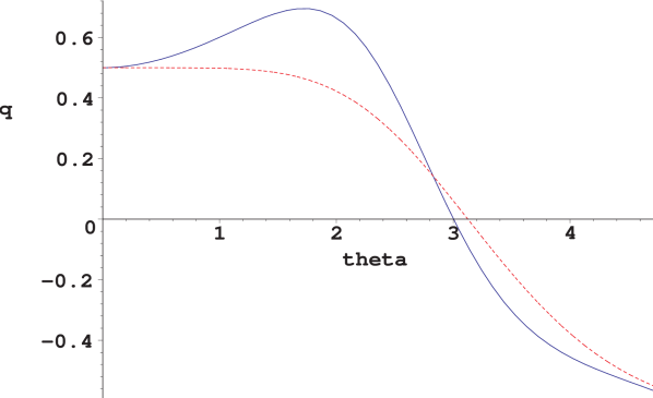
Figure 1: The deceleration parameter $q$ in the
toy model (blue, solid) and $\Lambda$CDM (red, dashed).

The explanation of the paradox that collapse induces acceleration is simple. The overdense region slows down the average expansion rate (11). As the volume fraction of the overdense region decreases, the contribution of the underdense region will eventually dominate, and the expansion rate will rise. This clarifies the equations (7), (10): larger variance of the expansion rate means that the volume fraction of the fastest expanding region rises more rapidly, contributing to acceleration. In fact, the deceleration parameter $q$ can become arbitrarily negative: $q<-1$ does not require violation of the null energy condition, unlike in FRW models.

While the overdense region is essential for acceleration, it is the underdense region which raises $Ht$ above the FRW value: unlike in $\Lambda$CDM, these two effects are distinct. The fact that gravity is attractive implies that acceleration driven by inhomogeneities satisfies $Ht<1$ [6]. One consequence is that acceleration cannot be eternal, as is physically clear: acceleration erases inhomogeneities, so their effect decreases, terminating acceleration. However, inhomogeneities can then become important again. In the real universe, where perturbations are nested inside each other with modes constantly entering the horizon, this could lead to oscillations between deceleration and acceleration.

Oscillating expansion could alleviate the coincidence problem, but structure formation does also have a preferred time near the era $\sim$ 10 billion years where acceleration has been observed. For cold dark matter, the size of structures which are just starting to collapse, relative to the horizon size, rises as structure formation proceeds, saturating once all perturbations which entered the horizon during the radiation-dominated era have collapsed. The size of structures becomes of the order of the maximum size around 10–100 billion years. This is encouraging with respect to the coincidence problem, as one would expect the corrections to the FRW equations to be strongest when collapsing regions are largest.

Outlook.

The possibility that sub-horizon perturbations could lead to acceleration has been explored before [7], and backreaction has been demonstrated with an exact toy model [8]. However, the conceptual issue of how average expansion can accelerate even though gravity is attractive -how gravity can look like anti-gravity- had been murky.

We have discussed how acceleration is intimately associated with gravitational collapse. This provides a link to structure formation, which in turn has a preferred time close to the observed acceleration era. Backreaction could thus provide an elegant solution to the coincidence problem, without new fundamental physics or parameters. To see whether this promise is realised, we should quantify the impact of structure formation on the expansion of the universe to make sure that we are fitting the right equations to increasingly precise cosmological observations.

References

References

- [1] Ellis G F R, Relativistic cosmology: its nature, aims and problems, 1983 The invited papers of the 10th international conference on general relativity and gravitation, p 215 Ellis G F R and Stoeger W, The ’fitting problem’ in cosmology, 1987 Class. Quant. Grav. 4 1697
- [2] Ellis G F R and Buchert T, The universe seen at different scales, 2005 Phys. Lett. A347 38 [gr-qc/0506106]
- [3] Buchert T, On average properties of inhomogeneous fluids in general relativity I: dust cosmologies, 2000 Gen. Rel. Grav. 32 105 [gr-qc/9906015]
- [4] Kerscher M, Buchert T and Futamase T, On the abundance of collapsed objects, 2001 Astrophys. J. 558 L79 [astro-ph/0007284]
- [5] Padmanabhan T, Structure formation in the universe, 1993 Cambridge University Press, Cambridge p 273
- [6] Räsänen S, Backreaction and spatial curvature in dust universes, 2006 Class. Quant. Grav. 23 1823 [astro-ph/0504005]
- [7] Räsänen S, Dark energy from backreaction, 2004 JCAP0402(2004)003 [astro-ph/0311257] Räsänen S, Backreaction of linear perturbations and dark energy [astro-ph/0407317]
- [8] Räsänen S, Backreaction in the Lemaître-Tolman-Bondi model, 2004 JCAP0411(2004)010 [gr-qc/0408097]