The Monitor project: Rotation of low-mass stars in the open cluster M34

Abstract

We report on the results of a $V$ and $i$-band time-series photometric survey of M34 (NGC 1039) using the Wide Field Camera (WFC) on the Isaac Newton Telescope (INT), achieving better than $1\%$ precision per data point for $13\la i\la 17$. Candidate cluster members were selected from a $V$ vs $V-I$ colour-magnitude diagram over $14<V<24$ ($0.12\la M/{\rm M}_{\odot}\la 1.0$), finding $714$ candidates, of which we expect $\sim 400$ to be real cluster members (taking into account contamination from the field). The mass function was computed, and found to be consistent with a log-normal distribution in ${\rm dN/dlogM}$. Searching for periodic variable objects in the candidate members gave $105$ detections over the mass range $0.25<M/{\rm M}_{\odot}<1.0$. The distribution of rotation periods for $0.4<M/{\rm M}_{\odot}<1.0$ was found to peak at $\sim 7\ {\rm days}$, with a tail of fast rotators down to periods of $\sim 0.8\ {\rm days}$. For $0.25<M/{\rm M}_{\odot}<0.4$ we found a peak at short periods, with a lack of slow rotators (eg. $P\ga 5\ {\rm days}$), consistent with the work of other authors (eg. Scholz & Eislöffel 2004) at very low masses. Our results are interpreted in the context of previous work, finding that we reproduce the same general features in the rotational period distributions. A number of rapid rotators were found with velocities $\sim$ a factor of two lower than in the Pleiades, consistent with models of angular momentum evolution assuming solid body rotation without needing to invoke core-envelope decoupling.

1 Introduction

M34 (NGC 1039) is a relatively well-studied intermediate-age open cluster ($\sim 200\ {\rm Myr}$, Meynet, Mermillod & Maeder 1993; Jones & Prosser 1996), at a distance of $\sim 470\ {\rm pc}$, distance modulus $(M-m)_{0}=8.38$ (Jones & Prosser, 1996), with low reddening: $E(B-V)=0.07\ {\rm mag}$ (Canterna, Crawford & Perry, 1979). The cluster is located at $\alpha={\rm 2^{h}42^{m}06^{s}}$, $\delta={\rm+42^{\circ}46^{\prime}}$ (J2000 coordinates from SIMBAD), corresponding to galactic coordinates $l=143.7^{\circ}$, $b=-15.6^{\circ}$.

Clusters in the age range between $\alpha$ Persei ($\sim 80\ {\rm Myr}$, Stauffer et al. 1999) and the Hyades ($\sim 625\ {\rm Myr}$, Perryman et al. 1998) are important for constraining stellar evolution models. A $1{\rm M}_{\odot}$ star reaches the zero age main sequence (ZAMS) at $\sim 30\ {\rm Myr}$, with progressively later spectral types reaching the ZAMS at later times. M34 is useful in this context owing to both its age and relative proximity, where we can study solar mass stars after evolving for a short time on the main sequence, and lower mass stars as they finish pre main sequence evolution. We estimate that $0.5\ {\rm M}_{\odot}$ stars reach the ZAMS at approximately the age of M34, using the models of Baraffe et al. (1998).

Membership surveys of M34 using proper motions (Ianna & Schlemmer 1993, Jones & Prosser 1996) have been carried out using photographic plates down to $V\sim 16.2$ ($M\sim 0.7\ {\rm M}_{\odot}$), finding a mean cluster proper motion of $\sim 20\ {\rm mas\ yr^{-1}}$. Studies of M34 members in the literature include spectroscopic abundance measurements for G and K dwarfs, finding a mean cluster metallicity $[{\rm Fe/H}]=+0.07\pm 0.04$ (Schuler et al., 2003). Rotation studies have used both spectroscopy (Soderblom, Jones & Fischer, 2001), covering the high- to intermediate-mass end of the M34 cluster members, down to G spectral types, and photometry (Barnes, 2003). Finally, a ROSAT soft X-ray survey (Simon, 2000), detected $32$ sources.

The existing surveys in M34 have concentrated on the high-mass end of the cluster sequence (typically K or earlier spectral types). Later spectral types, in particular M, down to the substellar regime, are not well-studied. A catalogue of low-mass M34 members could be used to perform both photometric (eg. surveys for rotation and eclipses) and spectroscopic (eg. spectral typing and metal abundance) studies of the K and M dwarf populations.

1.1 Evolution of stellar angular momentum

The early angular momentum distribution of young stars is commonly explained as resulting from an initial intrinsic angular momentum distribution consisting of relatively mild rotators (eg. with rotational periods of $\sim 8\ {\rm days}$ for typical very young classical T Tauri stars such as the population of slow rotators in the ONC, Herbst et al. 2002), modified by subsequent spin-up of the star during contraction on the PMS. Observations indicate that a fraction of the stars spin slower than expected due to contraction, suggesting that they are prevented from spinning up. The most popular explanation for this is disc locking (eg. Königl 1991, Bouvier, Forestini & Allain 1997, Collier Cameron, Campbell & Quaintrell 1995). In the T-Tauri phase, stars are still surrounded by accretion discs, so a star could retain a constant rotation rate during contraction due to angular momentum transport via magnetic interaction of the star and disc. The stars are thus prevented from spinning up until the accretion disc dissolves. Recent evidence in favour of this hypothesis has been obtained from Spitzer studies, eg. Rebull et al. (2006).

Very young clusters such as the Orion Nebula Cluster (ONC, age $\sim 1\pm 1\ {\rm Myr}$, Hillenbrand 1997) provide an ideal testing ground for these models. Herbst et al. (2002) found a bimodal period distribution in this cluster for $M>0.25{\rm M}_{\odot}$, with short- and long-period peaks, where the long-period peak corresponds to stars which are still locked to their circumstellar discs, preventing spin-up, whereas the stars comprising the short-period peak have had time to spin-up since becoming unlocked from their discs. The distribution appeared to be unimodal at low-masses ($M<0.25{\rm M}_{\odot}$) with only a short-period peak, implying that all of the low-mass stars were fast rotators and presumably not disc-locked.

After the accretion discs dissolve (by $20\ {\rm Myr}$ for $90\%$ of stars, see also Haisch, Lada & Lada 2001), the stars are free to spin up as they contract on the PMS. During this phase of the evolution, the stellar contraction dominates the angular momentum distribution. Disc lifetimes can be constrained by examining the rotation period distributions in this age range.

As the stars approach the zero-age main sequence (at $\sim 30-100\ {\rm Myr}$ for G and K spectral types), the contraction rate slows, and angular momentum losses begin to dominate. These are thought to result from magnetised stellar winds (Weber & Davis, 1967) and cause the stars to spin down gradually on the main sequence. Previous studies (eg. see Stassun & Terndrup 2003 for a recent review) have shown that most stars in young clusters ($\sim 100\ {\rm Myr}$) rotate slowly ($v\sin i<20\ {\rm km\ s^{-1}}$), but a minority rotate much faster ($v\sin i\sim 200\ {\rm km\ s^{-1}}$ for the fastest rotators). Moving to older clusters such as the Hyades ($\sim 625\ {\rm Myr}$, Perryman et al. 1998), nearly all of the velocities of G and K stars have fallen to $\la 10\ {\rm km\ s^{-1}}$. This process must have occurred over the age range ($\sim 200\ {\rm Myr}$) in which M34 lies.

The observations indicate that there is a large convergence in rotation rate from the Pleiades ($\sim 125\ {\rm Myr}$, Stauffer, Schultz & Kirkpatrick 1998) to the Hyades, but with little change for the slowest rotators. The change in rotation rate is also found to be mass-dependent, in the sense that lower-mass stars require lower angular momentum loss rates in order to reproduce the observations (Barnes & Sofia, 1996). In terms of the models, assuming solid body rotation, in the simplest Skumanich (1972) model the angular momentum evolves as the $-1/2$ power of the age $t$ of the star. This does not reproduce the observed convergence in rotation rates, or the mass-dependence. Furthermore, the observations appear to require a steeper early evolution than $t^{-1/2}$, followed by a flattening at later times.

Core-envelope decoupling (eg. Soderblom et al. 1993b) has been invoked to explain these observations. In the core-envelope decoupling scenario, the stars undergo differential rotation. While the core is decoupled from the envelope, all the angular momentum that is lost to the outside is taken from the envelope only. This rapidly spins down the surface layers, giving rise to the observed steep early evolution, while the core retains a high rotation rate. Later, as the core and envelope are gradually recoupled, the core effectively acts as a reservoir of angular momentum, giving rise to the observed flattening of the rotational evolution. These models are constrained by the situation in the sun, which is approximately a solid body rotator, ie. no differential rotation, so the decoupling must evolve out (see also Eff-Darwich, Korzennik & Jiménez-Reyes 2002 and references therein).

Results from more comprehensive models assuming solid body rotation are now able to provide an alternative explanation for the observations. For example, in the models of Bouvier et al. (1997), the more rapid spin-down of faster rotators (and hence convergence in rotation rates) can be explained in terms of their adopted angular momentum loss law, without requiring core-envelope decoupling, and the longer spin-down timescale for low-mass stars is explained by mass-dependent saturation of the angular momentum losses. In the $\alpha-\omega$ dynamo model, the mass dependency is a natural consequence of assuming that the saturation in angular momentum losses results from saturation of the dynamo itself. Alternatively, Giampapa et al. (1996) have suggested that that fully-convective stars have complex magnetic field geometries, mostly consisting of small loops contributing little to angular momentum losses. The change in magnetic field geometry toward lower-mass stars, with more closed loops, could then also give rise to a mass-dependent saturation of the angular momentum losses.

A review of these ideas is given in Bouvier (1997), based on the results of $v\sin i$ measurements in a number of open clusters, including $\alpha$ Persei, the Pleiades and the Hyades.

Recent work has been carried out at lower masses, eg. Scholz & Eislöffel (2004), who measured rotation periods for 9 very low-mass (VLM) Pleiades members with $0.08<M/{\rm M}_{\odot}<0.25$. They found a lack of slow rotators, with observed rotation periods from $\sim 0.012-1.7\ {\rm days}$, tending to increase linearly with mass. The implications of these results are that any angular momentum loss experienced by VLM stars must be very small, to preserve the high rotation velocities, or equivalently, the braking timescale of VLM stars is longer than that of higher-mass stars. These results lend weight to the idea that angular momentum loss is a strong function of stellar mass, and weakens towards the VLM regime (eg. Krishnamurthi et al. 1997 for solar-mass stars and Bouvier et al. 1997).

Mid- to low-mass stars ($0.4\la{\rm M}/{\rm M}_{\odot}\la 1.0$) in intermediate-age clusters such as M34 have experienced a period of evolution after the PMS spin-up, and are thus ideal for constraining spin-down timescales on the early main sequence. At very low-mass, we can also examine the late PMS angular momentum evolution.

1.2 The survey

We have undertaken a photometric survey in M34 using the Isaac Newton Telescope (INT). Our goals are three-fold: first, to establish a catalogue of candidate low-mass M34 members, second, to study rotation periods in a sample of these low-mass members, and third, to look for eclipsing binary systems containing low-mass stars, to obtain dynamical mass measurements in conjunction with radial velocities from follow-up spectroscopy. Such systems provide the most accurate determinations of fundamental stellar parameters (in particular, masses) for input to models of stellar evolution, which are poorly constrained in this age range. We defer discussion of our eclipsing binary candidates to a later paper once we have obtained suitable follow-up spectroscopy.

These observations are part of a larger photometric monitoring survey of young open clusters over a range of ages and metalicities (the Monitor project, Hodgkin et al. 2006 and Aigrain et al., in prep).

The remainder of the paper is structured as follows: the observations and data reduction are described in §2, and the colour magnitude diagram (CMD) of the cluster and candidate membership selection are presented in §3. The method we use for obtaining photometric periods is presented in §4, and the resulting rotation periods and amplitudes are discussed in §5. Finally, we summarise our conclusions in §6.

2 Observations and data reduction

Photometric monitoring data were obtained using the $2.5\ {\rm m}$ INT, with the Wide Field Camera (WFC) during a 10-night observing run in November 2004. This instrument provides a field of view of approximately $34^{\prime}\times 34^{\prime}$ at the prime focus of the INT, over a mosaic of four $2{\rm k}\times 4{\rm k}$ pixel CCDs, with $\sim 0.33^{\prime\prime}$ pixels. Our primary target was the Orion Nebula Cluster (ONC), which was observable for only half the night from La Palma, so the first $\sim 4.5\ {\rm hours}$ of each night were used to observe M34.

Monitoring was carried out using alternating $60\ {\rm s}$ $V$-band and $30\ {\rm s}$ $i$-band exposures, giving an observing cadence of $\sim 3.5\ {\rm minutes}$, over a $\sim 0.3\ {\rm sq.deg}$ region of the cluster. We also obtained $\sim 2\times$ $300\ {\rm s}$ $H\alpha$ exposures per night. Data were obtained on a total of 8 out of the 10 nights (many of these were partial due to poor weather), giving $275$ $V$-band and $268$ $i$-band frames after rejection of observations influenced by technical problems (image trailing), and $6$ $H\alpha$ frames. Our observations are sufficient to give an RMS per data point of $1\%$ or better down to $i\sim 17$, with saturation at $i\sim 13$ (see Figure 1), corresponding to a range of spectral types for M34 members from mid-G to early-M.

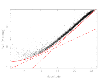
Figure 1: Plot of RMS scatter per data point as a function of magnitude for the $i$-band observations of M34, for all unblended objects with stellar morphological classifications. The diagonal dashed line shows the expected RMS from Poisson noise in the object, the diagonal dot-dashed line shows the RMS from sky noise in the photometric aperture, and the dotted line shows an additional $1.5\ {\rm mmag}$ contribution added in quadrature to account for systematic effects. The solid line shows the overall predicted RMS, combining these contributions.

For a full description of our data reduction steps, the reader is referred to Irwin et al. (in prep). Briefly, we used the pipeline for the INT wide-field survey (Irwin & Lewis, 2001) for 2-D instrumental signature removal (crosstalk correction, bias correction, flatfielding, defringing) and astrometric and photometric calibration. We then generated the master catalogue for each filter by stacking $20$ of the frames taken in the best conditions (seeing, sky brightness and transparency) and running the source detection software on the stacked image. The resulting source positions were used to perform aperture photometry on all of the time-series images. We achieved a per data point photometric precision of $\sim 2-5\ {\rm mmag}$ for the brightest objects, with RMS scatter $<1\%$ for $i\la 17$ (see Figure 1), corresponding to $\sim 1100$ unblended stars.

Our source detection software flags as likely blends any objects detected as having overlapping isophotes. This information is used, in conjunction with a morphological image classification flag also generated by the pipeline software (Irwin & Lewis, 2001) to allow us to identify non-stellar or blended objects in the time-series photometry.

Photometric calibration of our data was carried out using regular observations of Landolt (1992) equatorial standard star fields in the usual way. This is not strictly necessary for the purely differential part of a campaign such as ours, but the cost of the extra telescope time for the standards observations is negligible, for the benefits of providing well-calibrated photometry (eg. for the production of CMDs).

Lightcurves were extracted from the data for $\sim 14,000$ objects, $8500$ of which had stellar morphological classifications, using our standard aperture photometry techniques, described in Irwin et al. (in prep). We fit a 2-D quadratic polynomial to the residuals in each frame (measured for each object as the difference between its magnitude on the frame in question and the median calculated across all frames) as a function of position, for each of the $4$ WFC CCDs separately. Subsequent removal of this function accounted for effects such as varying differential atmospheric extinction across each frame. Over a single WFC CCD, the spatially-varying part of the correction remains small, typically $\sim 0.02\ {\rm mag}$ peak-to-peak. The reasons for using this technique are discussed in more detail in Irwin et al. (in prep).

For the production of deep CMDs, we stacked 120 observations in each of $V$ and $i$, taken in good seeing and sky conditions (where possible, in photometric conditions). Since there were insufficient observations taken in truly photometric conditions, the stacked frames were corrected for the corresponding error in the object magnitudes by comparing to a reference frame in known photometric conditions, and using the common objects to place stacked frames on the correct zero-point system. The required corrections were typically $\la 0.5\ {\rm mag}$. The limiting magnitudes, measured as the approximate magnitude at which our catalogues are $50\%$ complete, on these images were $V\simeq 23.4$ and $i\simeq 22.6$. For $H\alpha$ we stacked all of the observations taken in sufficiently good conditions ($4$ frames), giving a limiting magnitude of $H\alpha\simeq 21.7$ A single $600\ {\rm s}$ $r$-band frame was also taken, with a limiting magnitude of $r\simeq 22.1$.

3 Selection of candidate low-mass members

The first step in our survey is to identify the likely low-mass cluster members. The proper motion surveys discussed in §1 are not suitable because they become incomplete at the bright end of our magnitude range, eg. $V\ga 13$ assuming an apparent distance modulus to M34 of $8.60$, estimated from Figure 8 of Jones & Prosser (1996). We have therefore used colour-magnitude diagrams (CMDs) to search for candidate low-mass members in M34.

Since we only have optical photometry available over the whole mass range, the analysis here is preliminary and yields candidate cluster members only. We plan to make use of follow-up near-IR observations and spectroscopy to improve the rejection of field stars, and will publish a more detailed membership survey of M34 in due course.

3.1 The $V$ versus $V-I$ CMD

A $V$ versus $V-I$ CMD of M34 was produced for selecting the candidate cluster members, and is shown in Figure 2. The INT/WFC $V$ and $i$ measurements were converted to the Johnson-Cousins system of Landolt (1992) using colour equations derived from a large number of standard star observations, from the INT Wide Field Survey web pages:

$$(V-I) = (V_{ccd}-i_{ccd})\ /\ 0.894$$ (1)

$$V = V_{ccd}+0.005\ (V-I)$$ (2)

$$I = i_{ccd}-0.101\ (V-I)$$ (3)

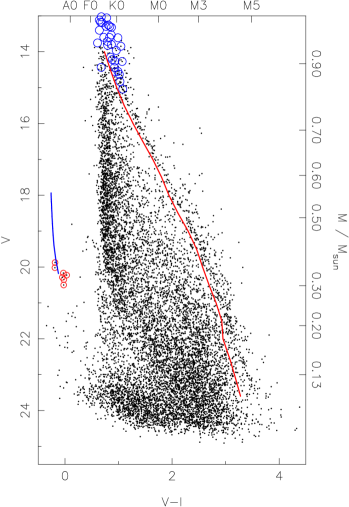
Figure 2: $V$ versus $V-I$ CMD of M34 from stacked images, for all objects with stellar morphological classification. The cluster main sequence is clearly visible on the right-hand side of the diagram. The cut used to select candidate photometric members is shown as the solid line (all objects above and to the right were selected). The objects in our sample assigned membership probabilities $P>80\%$ by Jones & Prosser (1996) are shown as open circles. The mass scale is from the $200\ {\rm Myr}$ NextGen model isochrone (Baraffe et al., 1998), using our empirical isochrone to convert the $V$ magnitudes to $I$ magnitudes, and subsequently obtaining the masses from these, due to known problems with the $V$ magnitudes from the models (see §3.1). The solid line and small circles at the lower left of the diagram show the models of Bergeron et al. (private communication) at the distance modulus of M34, for $\log g=8.5$ to an age of $250\ {\rm Myr}$, and our $7$ white dwarf candidates (see §3.6).

Candidate cluster members were selected by defining an empirical main sequence. This was initially done ‘by eye’ and refined from the initial guess by computing an iterative $k\sigma$ clipped median in $1\ {\rm mag}$ bins of $V$ magnitude, spaced at $0.5\ {\rm mag}$, down the CMD from $V=14$ to $24$ (the range over which the main sequence was clearly defined on the diagram). The result is given in Table 1. A cut was defined by moving this line perpendicular to the mean gradient of the main sequence, toward the faint, blue end of the diagram, by $0.1\ {\rm mag}+k\sigma(V-I)$ with $k=2$, where $\sigma(V-I)$ is the photometric error in $V-I$. The resulting curve is shown in Figure 2. The choice of $k$ is somewhat arbitrary, and was made to give a good separation between cluster members and field stars. A greater main sequence ‘width’ was allowed at the faint end to account for the increase in photometric errors.

$(V-I)_{0}$	$M_{V}$
0.737	5.4
0.849	5.9
0.970	6.4
1.110	6.9
1.277	7.4
1.458	7.9
1.648	8.4
1.814	8.9
1.953	9.4
2.125	9.9
2.317	10.4
2.479	10.9
2.598	11.4
2.723	11.9
2.865	12.4
2.983	12.9
3.020	13.4
3.180	13.9
3.309	14.4
3.451	14.9

Table 1: M34 empirical main sequence in dereddened $V-I$ colour and absolute $V$ magnitude. These values were computed assuming a cluster reddening of $E(B-V)=0.07$ and distance modulus $(M-m)_{0}=8.38$.

Accepting all objects brighter and redder than the empirical main sequence ensures that multiple systems (eg. binaries), which lie to this side of the main sequence, are not excluded. Examining the M34 CMD in Figure 2 indicates that the additional contamination compared to applying a restrictive cut on the red side is not significant. Using the technique described, we found $714$ candidate members.

We also considered using the model isochrone of Baraffe et al. (1998) for selecting candidate members. The model isochrone was found to be unsuitable due to the known discrepancy between the NextGen models and observations in the $V-I$ colour for $T_{\rm eff}\la 3700\ {\rm K}$ (corresponding here to $V-I\ga 2$). This was examined in more detail by Baraffe et al. (1998), and is due to a missing source of opacity at these temperatures, leading to overestimation of the $V$-band flux. Consequently, when we have used the NextGen isochrones to determine model masses and radii for our objects, the $I$-band absolute magnitudes were used to perform the relevant look-up, since these are less susceptible to the missing source of opacity, and hence give more robust estimates.

3.2 Completeness

The completeness of our source detection was estimated by inserting simulated stars as random $x,y$ positions into our images, drawing the stellar magnitudes from a uniform distribution. Figure 3 shows the resulting plot of completeness as a function of $V$-band magnitude. The completeness for objects on the M34 cluster sequence is close to $100\%$ up to the termination of the empirical main sequence line at $V\sim 23$ ($I\sim 20$).

Figure 3: Completeness in our source detection, measured as the fraction of simulated objects which were detected in each magnitude bin. The diagram is plotted in the Johnson $V$ system assuming objects to lie on the empirically-derived cluster main sequence track of §3.1 and Figure 2. The plot has been made only to $V=23$, corresponding to the termination of the empirical main sequence here.

3.3 Contamination

In order to estimate the level of contamination in our catalogue, we used the Besançon galactic models (Robin et al., 2003) to generate a simulated catalogue of objects passing our selection criteria at the galactic coordinates of M34 ($l=143.7^{\circ}$, $b=-15.6^{\circ}$), covering the WFC FoV of $\sim 0.29\ {\rm sq.deg}$ (including gaps between detectors). We selected all objects over the apparent magnitude range $13<V<24$, giving $7625$ stars. The same selection process as above for the cluster members was then applied to find the contaminant objects. A total of $283$ simulated objects passed these membership selection criteria.

In order to account for the effects of completeness in our source detection, the list of stellar magnitudes from the models was used to insert simulated stars at random $x,y$ positions into our $i$-band master image. We then ran the source detection software on the resulting simulated image, and kept all the inserted sources that were detected, in order to simulate the detection process, leaving a total of $279$ contaminant field stars. This gave an overall contamination level of $\sim 39\%$, and Figure 4 shows the contamination as a function of $V$ magnitude. We note that this figure is somewhat uncertain due to the need to use galactic models. Follow-up data will be required to make a more accurate estimate.

Figure 4: Contamination, measured as the ratio of the calculated number of objects in each magnitude bin from the galactic models, to the number of objects detected and classified as candidate cluster members in that magnitude bin. $1\sigma$ Poisson error bars are shown.

3.4 Near-IR CMD

In order to check our candidate membership assignments, we used the $K$-band data for M34 from the Point Source Catalogue (PSC) of the Two-Micron All-Sky Survey (2MASS) to obtain $K$-band magnitudes for our bright sources (2MASS is complete to $K\sim 14.3$, corresponding to $I\sim 16.5$, $V\sim 18.5$, or $\sim{\rm M2}$ spectral types in M34). Figure 5 shows a colour-magnitude diagram of $K$ versus $I-K$.

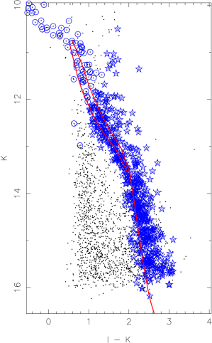
Figure 5: $K$ versus $I-K$ CMD of M34, for all objects with stellar morphological classification. $K$ magnitudes are plotted in the CIT system (Elias et al. 1982, Elias et al. 1983). Objects classified as members in Jones & Prosser (1996) are shown as open circles, and our photometrically selected candidate members are shown as five-pointed stars. The solid lines show the $200\ {\rm Myr}$ NextGen isochrones of Baraffe et al. (1998) for solar metallicity, with mixing length parameters $L_{\rm mix}=H_{P}$ (upper line) and $L_{\rm mix}=1.9H_{P}$ (lower line), where the larger $L_{\rm mix}$ makes a significant difference at high masses ($M\ga 0.6{\rm M}_{\odot}$).

The locations of our photometrically-selected candidate cluster members lie along the NextGen isochrone in Figure 5, indicating that our candidate member selection worked reasonably well over the magnitude range covered by the 2MASS data.

3.5 Alternative methods

We examined alternative methods for membership selection. The use of colour-colour diagrams to reduce contamination was suggested, but found to be of limited use for selection of candidate cluster members, compared to the standard CMD method we used above. The proper motion of M34 is $\sim 20\ {\rm mas\ yr^{-1}}$ (eg. Jones & Prosser 1996). We examined the possibility of using photographic data-sets (in particular the two Palomar Observatory Sky Survey epochs), but the dispersion in the proper motions of $\sim 60\ {\rm mas\ yr^{-1}}$ for the field objects (Jones & Prosser, 1996) combined with uncertainties $\sim 10\ {\rm mas\ yr^{-1}}$ at $I>16$ are too large to allow a clean separation of the cluster from the field for our targets. The only suitable comparison data-set for a significant sample of new proper motions is 2MASS, with a $\sim 5\ {\rm yr}$ baseline, ie. total motion of $0.1^{\prime\prime}$, smaller than the RMS astrometric errors. A proper motion study would be feasible in $\sim 15\ {\rm years}$ from the time of writing, when the motion would amount to $\sim 0.4^{\prime\prime}$ (which should be measurable given the $\sim 0.1^{\prime\prime}$ RMS accuracy of 2MASS). We can nevertheless use proper motions for weeding out rapidly-moving foreground objects, and intend to do this for the final membership analysis.

In terms of angular size and density of sources, M34 would be an ideal target for a radial velocity survey using multi-object spectroscopy on $4$ or $8\ {\rm m}$ class telescopes. Obtaining radial velocities (RVs) for a large sample of our candidate members could be used to improve the membership selection, using relatively low dispersion, eg. $R\sim 10,000$ given the cluster RV of $\sim-8\ {\rm kms^{-1}}$ (estimated from Table 3 of Jones & Prosser 1996).

3.6 White dwarfs

A number of faint, blue objects are visible in the CMD of Figure 2. White dwarfs (WDs) in M34 lie in this region of the diagram, with the WD cooling tracks of Bergeron et al. (private communication) shown as a line on Figure 2. At such young ages, we may be able to learn about the evolution of young, massive stars from these objects. We have selected $7$ objects in the CMD lying in the region occupied by WDs at the distance of M34 as candidate WD members, to be confirmed spectroscopically.

3.7 Luminosity and mass functions

We have calculated preliminary luminosity and mass functions using the photometric selection. Final versions will be published after we have obtained sufficient additional data to more reliably determine membership for our candidates.

The contamination-corrected luminosity function for M34 is shown in Figure 6 and tabulated in Table 2, computed from our catalogue of candidate cluster members. Note that the plot range was chosen to correspond to the range over which our sample is close to $100\%$ complete (see Figure 3). The resulting luminosity function resembles the solar neighbourhood luminosity function of Reid, Gizis & Hawley (2002).

Figure 6: M34 luminosity function (solid line) in apparent $I$-band magnitude, corrected for contamination. Note that this function has not been corrected for incompleteness in the source detection and cluster membership selection, since the correction is very small over the magnitude range shown. See also §3.2 and Figure 3. The spectral types were determined from the $I$-band absolute magnitudes for young disc stars of Leggett (1992). The dashed line shows the solar neighbourhood luminosity function of Reid et al. (2002), converted to the $I$-band using our empirical cluster main sequence, and normalised to give the same total number of objects over the $I$-band magnitude range plotted.

$I_{1}$	$I_{2}$	$\langle I\rangle$	${\rm dN/dI}$	${\rm\sigma(dN/dI)}$
12	13	12.5	3	4
13	14	13.5	18	12
14	15	14.5	41	11
15	16	15.5	49	10
16	17	16.5	101	12
17	18	17.5	92	12
18	19	18.5	101	13
19	20	19.5	33	12
20	21	20.5	-3	3

Table 2: Tabulated contamination-corrected M34 luminosity function (as shown in Figure 6) in $1\ {\rm mag}$ bins. $I_{1}$ and $I_{2}$ denote the start and end of the bin in $I$, $\langle I\rangle$ the central $I$ value of the bin, and ${\rm\sigma(dN/dI)}$ gives the estimated uncertainty from Poisson counting errors.

The mass function for M34 has been computed over the range $0.1\la M/{\rm M}_{\odot}\la 2.5$ covered by the available data (our sample plus proper motion members of M34 from Jones & Prosser 1996) with close to $100\%$ completeness. The lower limit results from the drop in completeness at $I\simeq 20$ for our sample, and the upper limit from the upper mass limit of the models of Baraffe et al. (1998). The result is shown in Figure 7. In order to produce these distributions, the observed number counts from our survey were corrected for field star contamination using the Besançon model star counts of §3.3. For the data from Jones & Prosser (1996), we chose only those objects with membership probabilities $P>80\ \%$. The masses were computed from the $I$-band magnitudes using the models of Baraffe et al. (1998), using a linear extrapolation from the high-mass end for the brightest objects from Jones & Prosser (1996).

We find that a log-normal mass distribution of the form:

$${\rm dN/dlogM}\propto\exp\left[-{\left(\log M-\log M_{0}\right)\over{2\sigma^{2}}}\right]$$ (4)

is a good fit to the data in ${\rm dN/dlogM}$, parameterized by a mass at maximum ${\rm dN/dlogM}$ of $M_{0}=0.44\pm 0.31\ {\rm M}_{\odot}$ and $\sigma=0.66\pm 0.08$. These are in relatively good agreement with the values of $M_{0}\sim 0.3\ {\rm M}_{\odot}$ and $\sigma\sim 0.5$ derived by Moraux et al. (2005) for a sample of three young open clusters. It should be noted that our survey covered only the central part of the cluster, and it is likely that the low-mass members are distributed with a larger core radius than the higher-mass members, implying a bias toward higher masses. Unfortunately our present survey does not have sufficient sky coverage to resolve this problem. It should also be noted that these conclusions were made on the basis of measurements over a very small range in mass. More data at higher or lower masses would improve the situation and allow us to examine the mass function in greater detail.

Figure 7: M34 mass function in ${\rm dN/dlogM}$, corrected for contamination, made using the models of Baraffe et al. (1998) to calculate a mass for each object from the $I$ magnitude. The solid line shows a log-normal fit to ${\rm dN/dM}$, ie. a quadratic fit to $\log($dN/dlogM$)$, with parameters $M_{0}=0.44\ {\rm M}_{\odot}$ (the mass at maximum ${\rm dN/dM}$), and $\sigma=0.66$. We have used the catalogue of M34 proper motion members from Jones & Prosser (1996) to populate the two highest-mass bins. Note that the projected areas covered by these surveys are similar, but the centres are offset by a few arcminutes, so the actual coverage of M34 members may differ, which will affect the results for the upper two bins.

$\log_{10}M_{1}$	$\log_{10}M_{2}$	$\langle\log_{10}M\rangle$	${\rm dN/dlogM}$	${\rm\sigma(dN/dlogM)}$
-1.0	-0.8	-0.9	642	263
-0.8	-0.6	-0.7	1046	139
-0.6	-0.4	-0.5	633	84
-0.4	-0.2	-0.3	567	65
-0.2	0.0	-0.1	233	46
0.0	0.2	0.1	109	15
0.2	0.4	0.3	54	15

Table 3: Tabulated M34 mass function in ${\rm dN/dlogM}$. $M_{1}$ and $M_{2}$ denote the start and end of the bin in $M$, $\langle\log_{10}M\rangle$ the central $\log_{10}M$ value of the bin, and ${\rm\sigma(dN/dlogM)}$ gives the estimated uncertainty from Poisson counting errors.

4 Period detection

4.1 Method

The limited time baseline of only $10\ {\rm nights}$ for our observations is insufficient to make a detailed study of stellar rotation periods $\ga 10\ {\rm days}$. However, our observations have relatively good sensitivity to short-period ($\la 10\ {\rm days}$ for example) systems so a careful examination of the data for rotation and other periodic variability has been carried out.

Variable objects were selected using least-squares fitting of sine curves to the time series $m(t)$ (in magnitudes) for all sources in the CCD images, using the form:

$$m(t)=m_{dc}+\alpha\sin(\omega t+\phi)$$ (5)

where $m_{dc}$ (the DC lightcurve level), $\alpha$ (the amplitude) and $\phi$ (the phase) were free parameters at each value of $\omega$ over an equally-spaced grid of frequencies, corresponding to periods from $0.005-20\ {\rm days}$. The lower period limit was chosen to correspond to the cadence of our observations, and the upper limit to the observing window, estimating that we still have a chance of recovering the correct period after observing only half a cycle (see also §4.2). The output of this procedure is a ‘least-squares periodogram’, with the best-fitting period being the one giving the smallest reduced $\chi^{2}$.

All of the lightcurves were processed in this manner. In order to distinguish the variable objects from the non-variable objects, we used the reduced $\chi^{2}$, but evaluated by subtracting a smoothed, phase-folded version of each lightcurve at the best-fitting period. The smoothing was carried out using median filtering over a $51$ data-point window, followed by a linear boxcar filter over an $11$ data-point window to smooth out any high-frequency features. This procedure accounts for any non-sinusoidal (but otherwise periodic) features in the lightcurve, and we have found empirically that it is capable of detecting somewhat non-sinusoidal variables such as detached eclipsing binaries and even the transiting extrasolar planet OGLE-TR-56b (Konacki et al., 2003) from the published lightcurve data.

Periodic variable lightcurves were selected by evaluating the change in reduced $\chi^{2}$:

$$\Delta\chi^{2}_{\nu}=\chi^{2}_{\nu}-\chi^{2}_{\nu,smooth}>0.4$$ (6)

where $\chi^{2}_{\nu}$ is the reduced $\chi^{2}$ of the original lightcurve with respect to a constant model, and $\chi^{2}_{\nu,smooth}$ is the reduced $\chi^{2}$ of the lightcurve with the smoothed, phase-folded version subtracted. We used a simple cut in $\Delta\chi^{2}_{\nu}$ rather than $\Delta\chi^{2}_{\nu}/\sigma(\chi^{2})$ (where $\sigma(\chi^{2})$ is the RMS of the $\chi^{2}$ measure, depending only on the number of data points) because our error estimates are somewhat unreliable, and therefore $\sigma(\chi^{2})$ underestimates the true dispersion of the $\chi^{2}_{\nu}$ value for a featureless lightcurve.

The threshold of $\Delta\chi^{2}_{\nu}>0.4$ was chosen as follows. All of the $714$ lightcurves of candidate cluster members were examined by eye, looking for variability, and placing the objects into four bins: objects with clear periodic variability, objects with clear non-periodic variability, ambiguous cases, and non-variable lightcurves. The numbers of objects falling in each bin were $102$, $8$, $67$ and $537$, respectively. Figure 8 shows these objects on a diagram of $\Delta\chi^{2}_{\nu}$ as a function of magnitude.

Figure 8: $\Delta\chi^{2}_{\nu}$ as a function of $i$-band magnitude for candidate M34 cluster members. The horizontal line shows the threshold at $\Delta\chi^{2}_{\nu}>0.4$, with solid circles indicating objects with clear periodic variability, open circles indicating the ambiguous cases, and small points indicating objects without periodic variability (non-variable lightcurves or those showing irregular variability).

The threshold was chosen to select at least all of the clear periodic variables and the more significant of the ambiguous lightcurves. Applying the threshold gave $283$ detections, after also removing objects lying on bad pixels for more than $10\%$ of their lightcurve points, non-stellar objects (by morphological classification) and any object with data points spanning a range of less than $1/2$ of the orbital phase. Note that objects flagged as blended were not removed since a large fraction of these were sufficiently uncontaminated to still be used. Only three of the lightcurves classified as ambiguous were rejected, and these were visually confirmed to be poor detections that were not obviously variable.

After applying the threshold, the selected lightcurves were examined independently by eye, to select the final sample included here. A total of $105$ lightcurves were selected, with the remainder appearing non-variable or too ambiguous to be included.

Our periods derived from the selection procedure described were refined by using both the $V$ and $i$ band lightcurves simultaneously, fitting a separate set of coefficients $m_{dc}$, $\alpha$ and $\phi$ in each band, but combining the $\chi^{2}$ values to produce a periodogram taking both bands into account. We have not used this method for the detection process itself because it is difficult to simulate for evaluating completeness, necessitating assuming a relation between the $V$ and $i$-band amplitudes and magnitudes for the simulated objects. Furthermore, at the faint end, where the detection begins to become incomplete, the signal to noise in the $V$-band is very poor for cluster members, so using the $V$-band does not give any improvement.

4.2 Simulations

The large amount of human involvement in our selection procedure is difficult to simulate in an unbiased manner. Nevertheless, we have attempted to evaluate our selection biases by performing Monte Carlo simulations, injecting sinusoidal modulations into non-variable M34 lightcurves, selected by requiring $\chi^{2}_{\nu}<\langle\chi^{2}_{\nu}\rangle+3\sigma(\chi^{2}_{\nu})$ (calculated using robust MAD – median of absolute deviations from the median – estimators in $0.5\ {\rm mag}$ bins) to remove the most variable objects. These were then subjected to exactly the same selection procedure as the real lightcurves, detailed in §4.1, including examination by eye.

In order to reduce biases in the detection process resulting from ‘knowing’ that the modulations are real, modulations were not inserted into a fraction ($1/6$) of the lightcurves shown to the human. A larger fraction ($1/2$) would be more realistic but would increase the already rather large number of lightcurves that must be examined.

Each simulation was run following uniform distributions in $\log_{10}\ {\rm period}$ from $0.1$ to $20\ {\rm days}$, and a uniform distribution in mass from $1.0$ to $0.1\ {{\rm M}_{\odot}}$, the second satisfied by choosing lightcurves in the correct magnitude range for each $0.1\ {\rm M}_{\odot}$ bin. Phases $\phi$ were chosen at random in $0\leq\phi<2\pi$, and the exercise was repeated for three typical amplitudes, $0.01\ {\rm mag}$, $0.02\ {\rm mag}$ and $0.05\ {\rm mag}$, corresponding approximately to the range of values for M34 rotators that we detected. $\sim 2000$ periodic variable objects were simulated in each amplitude bin.

The results of the simulations are shown in Figure 9 as greyscale diagrams of completeness, reliability and contamination as a function of period and stellar mass. Broadly, our period detections are close to $100\%$ complete for $P<10\ {\rm days}$ and $M\ga 0.4\ {\rm M}_{\odot}$.

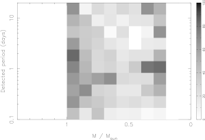
Figure 9: Results of the simulations for $0.02\ {\rm mag}$ amplitude as greyscale maps, where black corresponds to $100\%$ and white to $0\%$. The simulated region covered $0.2<{\rm M}/{\rm M}_{\odot}<1.0$ in order to be consistent with the M34 sample. Top panel: completeness as a function of real (input) period. Centre panel: Reliability of period determination, plotted as the fraction of objects with a given true period, detected with the correct period (defined as differing by $<20\%$ from the true period). Bottom panel: Contamination, plotted as the fraction of objects with a given detected period, having a true period differing by $>20\%$ from the detected value.

As with all ground-based observations, our period determinations suffer problems of aliasing. The most serious of these is at a frequency spacing of $1\ {\rm day^{-1}}$ corresponding to the observing gaps during the day, and leads to periodogram peaks at the ‘beat’ periods

$$1/P_{beat}=1/P\pm 1$$ (7)

where $P$ is the true period. Figure 10 illustrates this effect using our simulated lightcurves. Using both $V$ and $i$ bands to refine the period estimates mitigates the effect slightly (since the observations were not precisely simultaneous), but this has not been accounted for in the simulations.

Figure 10: Detected period as a function of actual (input) period for our simulations. Objects plotted with crosses had fractional period error $<10\%$, open circles $>10\%$. The straight line represents equal input and output periods. The curved lines are the loci of the $\pm 1\ {\rm day^{-1}}$ aliases from equation (7). The majority of the points fall either on (or close to) the line of equal periods, or on one of the curves consistent with $1\ {\rm day^{-1}}$ aliasing.

4.3 Detection rate and reliability

The locations of our detected periodic variable candidate cluster members on a $V$ versus $V-I$ CMD of M34 are shown in Figure 11. The diagram indicates that the majority of the detections lie on the single-star cluster main sequence, as would be expected for rotation in cluster stars as opposed to, say, eclipsing binaries.

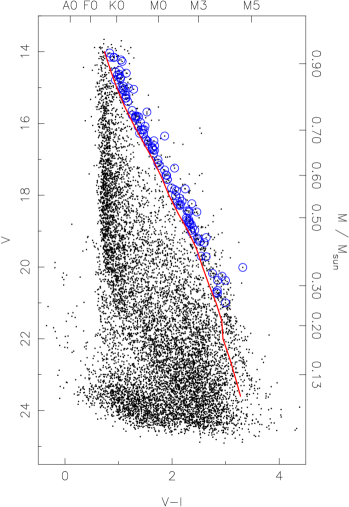
Figure 11: $V$ versus $V-I$ CMD of M34, for all objects with stellar morphological classification, as Figure 2, showing all $105$ candidate cluster members with detected periods (open circles).

Figure 12 shows the fraction of cluster members with detected periods as a function of $i$ magnitude. The rise from the bright end towards lower masses indicates that $M$-dwarfs may show more spot-related rotational variability within our detection limits than $K$ or $G$-dwarfs. This would be consistent with an increase in spot coverage moving to later spectral types. The decaying portion of the histogram from $i\sim 15$ is likely to be an incompleteness effect resulting from the gradual increase in the minimum amplitude of variations we can detect (corresponding to the reduction in sensitivity moving to fainter stars, see Figure 1) and not a real decline.

Figure 12: Fraction of candidate cluster members detected as periodic variables, plotted as a function of magnitude. This distribution has not been corrected for incompleteness in the period detections, so the decaying portion of the histogram from $i\sim 15$ is likely to be an incompleteness effect resulting from the gradual increase in the minimum amplitude of variations we can detect, as a function of increasing magnitude (and hence increasing noise, see Figure 1), and not a real decline.

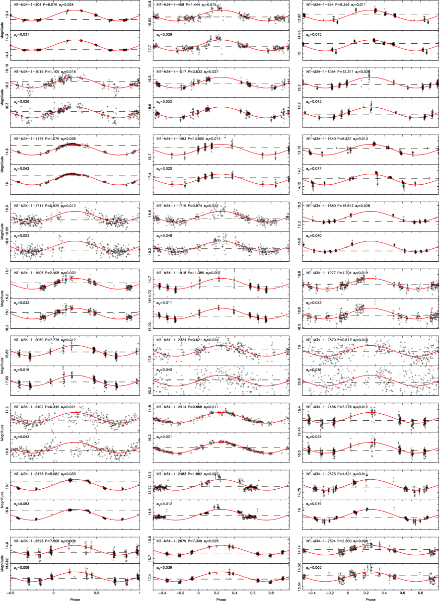
Figure 19: Phase-folded lightcurves of our $105$ periodic variables classified as candidate cluster members. The upper panel for each object shows the $i$-band lightcurve, the lower panel the $V$-band lightcurve. The dashed lines show the median flux level of the object, and the solid lines show the fitted sine curves. The lightcurves are labelled with period $P$ in days, and $\alpha_{i}$ and $\alpha_{V}$, the amplitudes in $i$ and $V$ bands, respectively. See also Table 5.

The phase-folded lightcurves of all our rotation candidates are shown in Figure 19, and their properties summarised in Table 5 (see Appendix A).

4.4 Non-periodic objects

The population of objects rejected by the period detection procedure described in §4 was examined, finding that the most variable population of these lightcurves (which might correspond to non-periodic or semi-periodic variability) was contaminated by a number of lightcurves exhibiting various uncorrected systematic effects. It is therefore difficult to quantify the level of non-periodic or semi-periodic variability in M34 from our data. Qualitatively however, there appear to be very few of these variables, and examining the lightcurves indicated only $\sim 3$ obvious cases, which strongly resembled eclipses (either planetary transits or eclipsing binaries), and will be the subject of a later Monitor project paper.

5 Results

5.1 Periods and rotational velocities

Period distributions for the objects photometrically selected as possible cluster members are shown in Figure 13, a plot of period as a function of $V-I$ colour is shown in Figure 14, and plots of period and amplitude as a function of mass are shown in Figures 15 and 16, respectively.

Figure 13: Period distributions for objects classified as possible photometric members, in three mass bins: $0.7\leq M/{\rm M}_{\odot}<1.0$ (corresponding roughly to late-G and K spectral types), $0.4\leq M/{\rm M}_{\odot}<0.7$ (early-M) and $M<0.4\ {\rm M}_{\odot}$ (late-M and VLM). The bottom right panel shows the period distribution for $0.4\leq M/{\rm M}_{\odot}<1.0$ plotted in $log_{10}$ period, indicating that the apparent bimodality in this mass range is probably not significant. The dashed lines show the measured period distributions, and the solid lines show the results of attempting to correct for incompleteness and reliability, as described in the text. Objects with periods flagged as unreliable in Table 5 have been excluded.

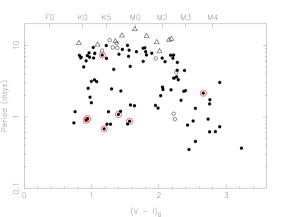
Figure 14: Plot of rotation period as a function of dereddened $V-I$ colour for M34. X-ray sources from Simon (2000) are overlaid with open circles. Open symbols indicate objects flagged ‘a’ (open circles) and ‘b’ (open triangles) in Table 5.

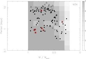
Figure 15: Plot of rotation period as a function of mass for the Pleiades (top) and M34 (bottom). Ages: $125\ {\rm Myr}$ (Stauffer, Schultz & Kirkpatrick, 1998) and $200\ {\rm Myr}$. Masses were interpolated from the model isochrones of Baraffe et al. (1998) using the $I$-band magnitudes (two Pleiades objects without this information were excluded). The Pleiades data are a compilation of the results from Van Leeuwen, Alphenaar & Meys (1987), Stauffer et al. (1987), Magnitskii (1987), Prosser et al. (1993a), Prosser et al. (1993b), Prosser et al. (1995), Krishnamurthi et al. (1998) (taken from the open cluster database), Terndrup et al. (1999) and Scholz & Eislöffel (2004). Symbols for M34 as Figure 14, with the greyscales showing the completeness for $0.02\ {\rm mag}$ periodic variations from Figure 9.

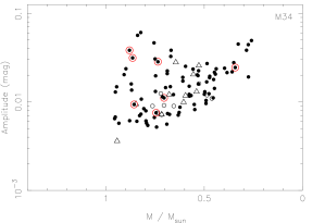
Figure 16: Plot of amplitude as a function of mass for the Pleiades (top) and M34 (bottom). The Pleiades amplitudes have been converted to the semi-amplitude as used in this work, and the passband used is indicated by the symbols: filled circles indicate $V$-band, crosses indicate $I$-band, and open circles denote objects with amplitudes measured in unknown passbands (but suspected to be $V$). All symbols in the M34 plot are as Figure 15 with all objects measured in i-band. The lower envelope of this diagram clearly traces the RMS curve in Figure 1 and therefore results from incompleteness at low amplitude for faint stars resulting from increased noise.

5.1.1 Period distributions

We have attempted to correct the period distribution for cluster members in Figure 13 for the effects of incompleteness and (un)reliability using the simulations described in §4.2. The results are shown in the solid histograms in Figure 13. This histogram was generated as follows: for each bin of the period distribution as a function of detected period, containing $N_{i}$ objects, we chose $N_{i}$ random objects falling in that bin from the simulations, and generated a new histogram using the real periods of the simulated objects. We then averaged over $1000$ realisations of this process. This has the effect of converting the histogram plotted as a function of detected period to one plotted as a function of real period. This was then corrected for incompleteness by dividing by the completeness fraction from Figure 9.

We applied two-sided Kolmogorov-Smirnov (K-S) tests to the corrected distributions in adjacent mass bins to evaluate whether the visible differences between the distributions were statistically significant. In particular, there is an apparent clear distinction between the distribution for $M>0.4\ {\rm M}_{\odot}$ and $M<0.4\ {\rm M}_{\odot}$, in the sense that there are few slow rotators at low-mass. The results are summarised in Table 4.

Mass range 1	Mass range 2	$P({\rm same})$
$0.7\leq M/{\rm M}_{\odot}<1.0$	$0.4\leq M/{\rm M}_{\odot}<0.7$	$0.85$
$0.4\leq M/{\rm M}_{\odot}<0.7$	$M<0.4\ {\rm M}_{\odot}$	$2\times 10^{-3}$

Table 4: Results of two-sided Kolmogorov-Smirnov tests to evaluate the probabilities that the period distributions in adjacent mass bins are drawn from the same parent population.

The K-S test for the first two mass bins is inconsistent with there being significant differences in the period distribution. However, the test for the $0.4\leq M/{\rm M}_{\odot}<0.7$ and $M<0.4\ {\rm M}_{\odot}$ bins indicates that they differ significantly at the $99.8\%$ confidence level, ie. the very low-mass stars ($M<0.4\ {\rm M}_{\odot}$) show a different period distribution than the higher-mass stars ($M>0.4\ {\rm M}_{\odot}$). This effect is also visible in Figure 15, and is discussed further in §5.1.5.

5.1.2 Bimodality?

The period distributions for $M>0.4\ {\rm M}_{\odot}$ in Figure 13 appear to be bimodal when plotted in linear period (see also Figure 15), but the apparent bimodality is much less obvious in $\log_{10}$ period (see the lower right panel of Figure 13). Following Stassun et al. (1999), we attempted to determine whether this bimodality is statistically significant by performing a one-sample Kolmogorov-Smirnov test against a model distribution, taken to be a simple function $N(P)=30(1-P/15)$, fit by eye to the upper envelope of the distribution, over $0<P<15\ {\rm days}$. The result was a $28\%$ probability that our period distribution was indeed drawn from this simple model distribution. The high probability for this poor model coupled with the results in $\log_{10}$ period implies that the apparent bimodality is not significant.

Truly bimodal distributions are typically seen only in much younger clusters (eg. the ONC, Herbst et al. 2002), although there is evidence that this may also be the case in the Pleiades (eg. Soderblom et al. 1993a) and are generally interpreted as resulting from the presence of a mixture of disc-locked and unlocked, spun-up stars (see §1.1). Such an interpretation cannot hold at the age of M34.

Interestingly, the presence of a short-period peak at $P\sim 1-2\ {\rm days}$ and a longer period peak at $P\sim 7\ {\rm days}$ is consistent with the empirical view on angular momentum evolution of Barnes (2003). Briefly, the short-period peak corresponds to the $C$ or ‘convective’ sequence, and the long-period peak to the $I$ or ‘interface’ sequence. In this interpretation, stars on the $C$ sequence have decoupled radiative and convective zones, with angular momentum loss due to stellar winds coupled to convective magnetic fields. On the $I$ sequence, an interface dynamo couples the zones leading to increased angular momentum loss (Barnes, 2003). Very low-mass stars (eg. $M<0.4\ {\rm M}_{\odot}$ in Figure 13) are fully convective, so they can only lie on the $C$ sequence and hence fall at short periods.

5.1.3 Rapid rotators

The presence of rapid rotation (eg. $P<1\ {\rm day}$) at the age of M34 is important for constraining models of angular momentum evolution, discussed in §5.2. We have examined the periods of these stars, to check that they are not rotating close to their break-up velocity, where they would be short-lived, suggestive of spin-up on the ZAMS. The corresponding critical period $P_{crit}$ for break-up is given approximately by:

$$P_{\rm crit}=0.116\ {\rm days}\ {(R/{\rm R_{\odot}})^{3/2}\over{(M/{\rm M_{\odot}})^{1/2}}}$$ (8)

where $R$ and $M$ are the stellar radius and mass respectively (eg. Herbst et al. 2002). Using the models of Baraffe et al. (1998), the object rotating closest to its critical period is M34-1-2402, at $P=0.260\ {\rm days}$, where $P_{\rm crit}=0.039\ {\rm days}$, a factor of $7$ shorter, so we find no objects in M34 rotating close to break-up.

5.1.4 $0.4-1.0\ {\rm M}_{\odot}$ objects

Comparing the distributions of rotational periods for M34 and the Pleiades in Figure 15 indicates that, in general, the M34 distribution resembles a “spun-down” Pleiades distribution, exactly as expected. However, several conspicuous objects are visible in Figure 15, with periods close to $1\ {\rm day}$ and high masses ($\sim 0.8-1.0\ {\rm M}_{\odot}$). These are somewhat difficult to explain by spin-down of faster Pleiades rotators, given the lack of $<1\ {\rm day}$ period rotators there for $M\ga 0.9\ {\rm M}_{\odot}$ (see Figure 15), but the discrepancy could result from $\sim 0.1\ {\rm M}_{\odot}$ errors in the computation of the masses, dominated by errors in determining the $I$ magnitudes (in particular for the Pleiades data, due to the conversions required between the photometric systems used by the various authors).

The lightcurves for these objects were examined carefully, finding two very significant detections at unusually large amplitude with associated X-ray sources, M34-1-2953 and M34-3-523. Detection in X-rays is suggestive of youth or binarity. Since these objects are at high-mass and hence subject to increased field contamination, it is possible that they may be field objects. One further object was detected in X-rays, M34-4-1092, with a $\sim 1\%$ amplitude, and interestingly is the only one of these objects lying away from the cluster sequence, being $\sim 0.5\ {\rm mag}$ brighter. We therefore suspect that it is a binary, to be confirmed spectroscopically. The remaining objects, M34-4-2697 and M34-4-2833, are two of our lowest amplitude rotation candidates ($\sim 0.5\%$) and are marginal detections. Our planned spectroscopy of all the candidates should allow us to weed out any field contaminants, and to measure $v\sin i$ for any very rapid rotators to confirm their nature.

On the suggestion of the anonymous referee, we note the strong resemblance between the M34 results in Figure 15 and the Pleiades $v\sin i$ distribution of Soderblom et al. (1993a). These authors also found the majority ($80\%$) of the rotators to have low velocities, with an upper branch of rapid rotators comprising the remainder of the sample.

Accounting for the differences in sensitivity between the surveys, Figure 16 shows no significant evolution in amplitude from the Pleiades to M34. However, we do find an apparent trend of decreasing amplitude moving to lower masses, down to $\sim 0.4\ {\rm M}_{\odot}$ in M34. It is not clear whether a similar trend exists in the Pleiades over this mass range due to the lack of data.

5.1.5 $<0.4\ {\rm M}_{\odot}$ objects

Figure 13 shows a clear and statistically significant lack of slow rotators in the period distribution for $M<0.4\ {\rm M}_{\odot}$. This appears to be a real effect, and is not caused, for example, by selection biases in our sample. This effect has been observed previously (eg. Scholz & Eislöffel 2004) at very low mass, but we were unable to find significant samples of rotation periods in the literature for the mass range $0.25<M/{\rm M}_{\odot}<0.4$ probed by our sample, so it is complementary to these previous studies.

Tentatively the data in this mass range suggest that the typical rotation periods of these stars decrease as a function of decreasing mass, ie. less massive stars are faster rotators. This is in good agreement with the results at very low mass ($M\la 0.25\ {\rm M}_{\odot}$) from Scholz & Eislöffel (2004), who found the rather slow spin-down of VLM stars to be better fit by models assuming an exponential angular momentum loss law, giving $P\propto{\rm e}^{t}$, rather than the Skumanich (1972) $t^{1/2}$ law that applies for higher-mass stars. They attribute this difference to the fully convective nature of the low-mass objects, which cannot support a large scale magnetic dynamo, which gives rise to the Skumanich (1972) angular momentum loss law in solar-mass stars. We cannot make a detailed assessment of these conclusions over the mass range $0.25<M/{\rm M}_{\odot}<0.4$, since we could not find a suitable equivalent large sample of stars with measured rotation periods in a young open cluster from the literature. This will be addressed by the Monitor project, where we have obtained photometric periods for low-mass stars in several young clusters, including NGC 2516 ($\sim 150\ {\rm Myr}$, Jeffries, Thurston & Hambly 2001), M50 ($\sim 130\ {\rm Myr}$, Kalirai et al. 2003) and NGC 2362 ($\sim 5\ {\rm Myr}$, Moitinho et al. 2001), to be presented in a future publication.

Scholz & Eislöffel (2004) found significantly lower amplitudes for $M<0.25\ {\rm M}_{\odot}$ than for the higher-mass ($M\ga 0.5\ {\rm M}_{\odot}$) Pleiades objects (see Figure 16). We see no evidence for this in the interval $0.25<M/{\rm M}_{\odot}<0.4$, finding instead amplitudes comparable to those of the stars in the higher-mass bin. We cannot test the result in M34 for $M<0.25\ {\rm M}_{\odot}$ with the present data-set.

5.1.6 Comparison with $v\sin i$ measurements

We have compared our sample of objects with the spectroscopic sample of Soderblom, Jones & Fischer (2001). Due to the different magnitude ranges, we only have $22$ objects in common, and obtained photometric periods for $12$ of these. The $10$ objects missed did not show significant periodic variability during visual examination of the lightcurves. Figure 17 shows a comparison of the $v\sin i$ values with $v_{\rm rot}$ derived from our photometric periods, derived as:

$$v_{\rm rot}=2\pi R/P$$ (9)

with stellar radii $R$ taken from the models of Baraffe et al. (1998).

Figure 17: Plot of the photometric rotation velocity $v_{\rm rot}$ as a function of the $v\sin i$ value measured by Soderblom, Jones & Fischer (2001). The diagonal line indicates the case where $v\sin i=v_{\rm rot}$, and the region above the line corresponds to the “allowed” region where $v\sin i<v_{\rm rot}$. The small population of objects with $v\sin i$ slightly greater than $v_{\rm rot}$ may result from over-estimation of the $v\sin i$ values and are close to the lower measurable limit for the spectroscopic observations of Soderblom, Jones & Fischer (2001). Alternatively, these could highlight deficiencies in the model radii we have used to derive $v_{\rm rot}$.

We note that the long-period end of all the figures presented in this section is somewhat affected by the short observing window we had available, and should therefore be treated with caution. Nevertheless, we believe that useful conclusions can still be drawn from the data.

5.2 Rotational evolution

The ranges of measured rotation periods in IC 2391, IC 2602, $\alpha$ Per, the Pleiades, M34 and the Hyades are compared in Figure 18. The samples for IC 2391 and IC 2602 have been combined due to the very similar distance moduli and ages of these clusters. We use the lower and upper $10\%$iles of the rotational period distributions to trace the evolution of the rapid and slow rotators, respectively. The convergence in rotation rates across the full age range from IC 2391 and IC 2602 at $\sim 30\ {\rm Myr}$ to the Hyades ($\sim 625\ {\rm Myr}$, Perryman et al. 1998) is clearly visible in the diagram, due to spin-down of the rapid rotators by a greater amount than the slow rotators. The diagram also indicates the differences in evolution between (roughly) K and M stars, although it is difficult to constrain the latter because the samples we have gathered from the literature in $\alpha$ Per and the Hyades are substantially incomplete at low masses.

Figure 18: Plot of the IC 2391, IC 2602 ($\sim 50\ {\rm Myr}$, Barrado y Navascués, Stauffer & Jayawardhana 2004), $\alpha$ Per ($\sim 80\ {\rm Myr}$, Stauffer et al. 1999), Pleiades, M34 (using all of our period detections to avoid biasing the distribution against long periods) and Hyades rotation periods as a function of time, in two mass bins: $0.7\leq M/{\rm M}_{\odot}<1.0$ (corresponding roughly to G and K spectral types) and $0.4\leq M/{\rm M}_{\odot}<0.7$ (early-M). A similar diagram was not plotted for the $M<0.4\ {\rm M}_{\odot}$ (late-M and VLM) bin of Figure 13 since there were no suitable samples in the other clusters covering the same mass range ($0.25<M/{\rm M}_{\odot}<0.4$). The upper and lower $10\%$iles of the period distributions, and their medians, are shown as short horizontal lines. The change in the median indicates the convergence toward long periods moving from the Pleiades, to M34, to the Hyades. The IC 2391 data were taken from Patten & Simon (1996) and IC 2602 from Barnes et al. (1999). The $\alpha$ Per data are a compilation of the results from Stauffer et al. (1985), Stauffer, Hartmann & Jones (1989), Prosser et al. (1993a), Prosser (1991), Prosser et al. (1993b), O’Dell & Collier Cameron (1993), Prosser et al. (1995), O’Dell, Hendry & Collier Cameron (1994), O’Dell at al. (1996), Allain et al. (1996), Martín & Zapatero Osorio (1997), Prosser & Randich (1998), Prosser, Randich & Simon (1998), Barnes et al. (1998), and the Hyades data from Radick et al. (1987) and Prosser et al. (1995), taken from the open cluster database. The solid lines show the predicted evolution from Equations 10 and 11 for a $0.8{\rm M}_{\odot}$ star in the left-hand panel, and a $0.6{\rm M}_{\odot}$ star in the right-hand panel. The dashed lines show only the $t^{1/2}$ angular momentum loss component from (11) for comparison.

We caution that the samples in Figure 18 were taken from a wide variety of sources and may not be directly comparable. The reliability of the long periods in our M34 sample may be reduced by our limited time base-line. For the rapid rotators, the $10\%$ile may be affected by field contamination (due to field objects misclassified as cluster members), for example contact binary systems, which have very short photometric periods, but are otherwise difficult to distinguish from rotational modulation at low amplitude.

The rotational evolution can be simply modelled by assuming that it results from two components: the spin-up due to contraction in stellar radius (while conserving total angular momentum) as a function of age, which we compute from the models of Baraffe et al. (1998), and spin-down resulting from angular momentum loss:

$$P_{2}=\alpha P_{1}\left(R_{2}/R_{1}\right)^{2}$$ (10)

where $P_{1}$ and $P_{2}$ are the rotation periods at the two ages, $R_{1}$ and $R_{2}$ are the corresponding stellar radii, and $\alpha$ is a multiplicative factor resulting from angular momentum loss.

The simple Skumanich (1972) law gives

$$\alpha_{\rm sk}=\left(t_{2}/t_{1}\right)^{1/2}$$ (11)

where $t_{1}$ and $t_{2}$ are the respective ages ($t_{1}<t_{2}$). The predictions of this model are compared with the observations in Figure 18. The results indicate that in general, the angular momentum loss law (11) loses angular momentum too slowly between the Pleiades and M34, and likewise for the fast rotators between M34 and the Hyades. It appears to lose angular momentum (slightly) too quickly for the slow rotators from M34 to the Hyades, although the latter conclusion depends on our measured slow rotation periods, which may be unreliable. We suggest that the observations require a more rapid spin-down from the Pleiades to M34, followed by flattening between M34 and the Hyades.

Our results do however appear to be consistent with more comprehensive models of angular momentum evolution assuming solid body rotation, for example Bouvier et al. (1997), where the maximum rotational velocity decreases from $v_{\rm max}=100\ {\rm km\ s^{-1}}$ ($P\sim 0.5\ {\rm days}$ at ${\rm M}_{\odot}$, ${\rm R}_{\odot}$) at the age of the Pleiades to $v_{\rm max}=50\ {\rm km\ s^{-1}}$ ($P\sim 1\ {\rm day}$) at the age of M34, roughly as observed. Models incorporating core-envelope decoupling (eg. Allain 1998, see also Figure 3 of Bouvier 1997 and Keppens, MacGregor & Charbonneau 1995) cause much less efficient braking on the ZAMS for the first few hundred Myr, giving rise to faster rotators at the age of M34 than we have detected for these masses.

6 Conclusions

We have reported on results of a photometric survey of M34 in $V$ and $i$ bands. Selection of candidate members in a $V$ versus $V-I$ colour-magnitude diagram using an empirical fit to the cluster main sequence found $714$ candidate members, over a $V$ magnitude range of $14<V<24$ ($0.12\la M/{\rm M}_{\odot}\la 1.0$). The likely field contamination level was estimated using a simulated catalogue of field objects from the Besançon galactic models (Robin et al., 2003), finding that $\sim 283$ objects were likely field contaminants, an overall contamination level of $\sim 39\%$, implying that there are $\sim 400$ real cluster members over this mass range in our field-of-view. The next step in our membership survey will be to combine our optical data with planned near-IR photometry and optical spectroscopy to reduce the contamination level.

The M34 mass function was examined over the range $0.1\la M/{\rm M}_{\odot}\la 1.0$ ($13<I<20$), finding that a log-normal function was a good description of the data in ${\rm dN/dlogM}$, with parameters $M_{0}=0.44\pm 0.31\ {\rm M}_{\odot}$ (the mass at maximum ${\rm dN/dM}$), and $\sigma=0.66\pm 0.08$.

From $\sim 8\ {\rm nights}$ of time-series photometry (many of which were partial) we derived lightcurves for $\sim 8500$ objects in the M34 field, achieving a precision of $<1\%$ over $13\la i\la 17$. The lightcurves of our candidate M34 cluster members were searched for periodic variability corresponding to stellar rotation, giving $105$ detections over the mass range $0.25<M/{\rm M}_{\odot}<1.0$.

The rotational period distribution for $0.4<M/{\rm M}_{\odot}<1.0$ was found to peak at $\sim 7\ {\rm days}$ with a tail of fast rotators having rotational periods down to $\sim 0.8\ {\rm days}$. Our data suggest that most of the angular momentum loss for stars with masses $\ga 0.4\ {\rm M}_{\odot}$ happens on the early main sequence, by the age of M34 ($\sim 200\ {\rm Myr}$), in particular for the slow rotators. We observed a number of rapidly-rotating stars ($v_{\rm rot}\sim 50-100\ {\rm km\ s^{-1}}$), finding in general that the results can be explained by models of stellar angular momentum loss assuming solid body rotation (eg. Bouvier et al. 1997) without needing to invoke core-envelope decoupling, which seems to give rise to faster rotators at the age of M34 than we have detected for these masses.

Our rotation period distribution for $0.25<M/{\rm M}_{\odot}<0.4$ was found to peak at short periods, with an lack of slow rotators (eg. $P\ga 5\ {\rm days}$). Our simulations indicate that the effect is real and does not result from a biased sample. This is consistent with the work of other authors (eg. Scholz & Eislöffel 2004) at very low masses.

The multi-band photometry we have obtained can be used to examine the properties of the star spots giving rise to the rotational modulations. This will be investigated in a future publication.

One of the major problems in our survey is field contamination. We intend to publish the final catalogue of M34 membership candidates after obtaining follow-up spectroscopy. However, the preliminary catalogue of membership candidates is available on request.

Appendix A Lightcurves and tabular data

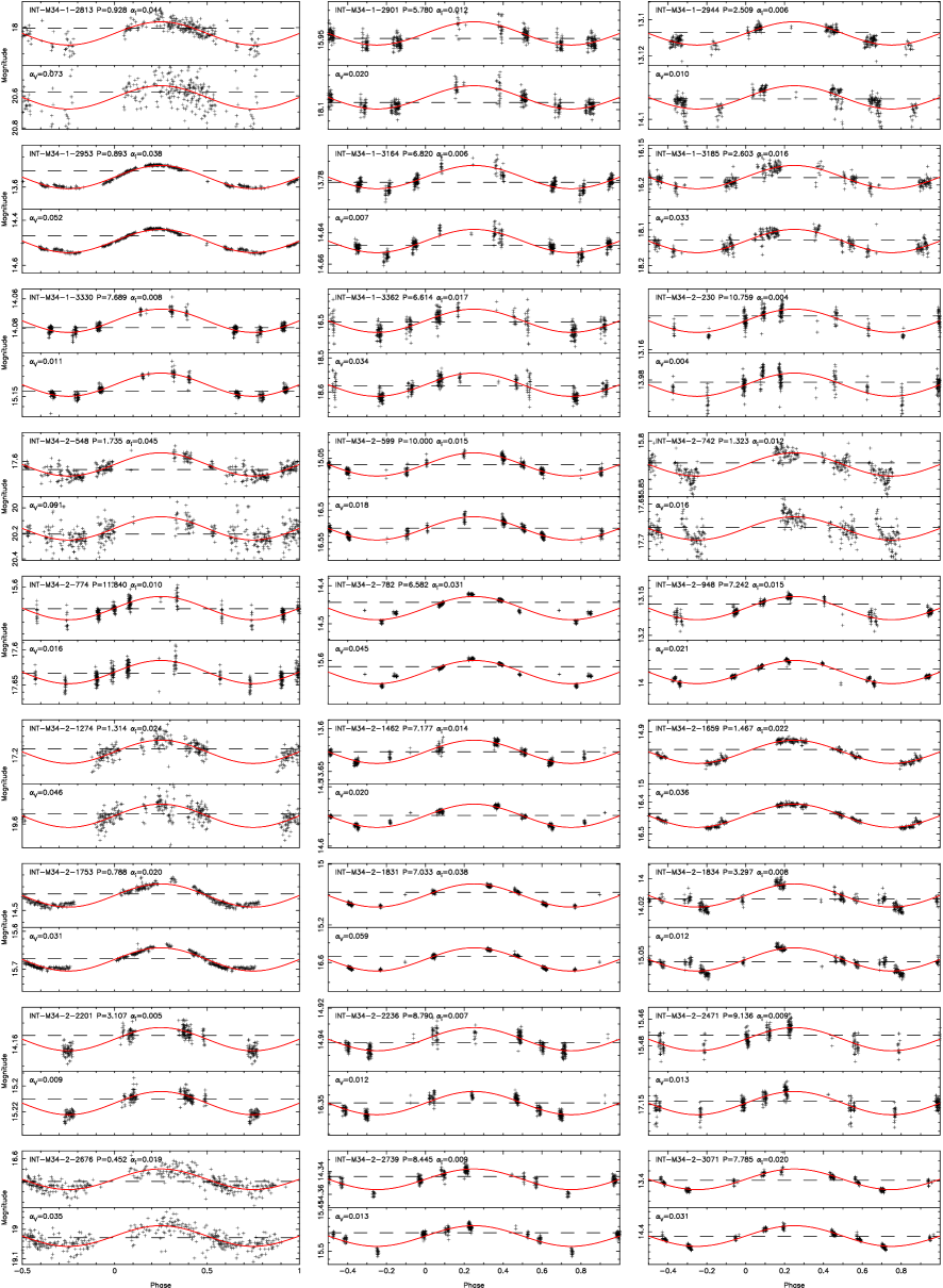
Figure 20: continued

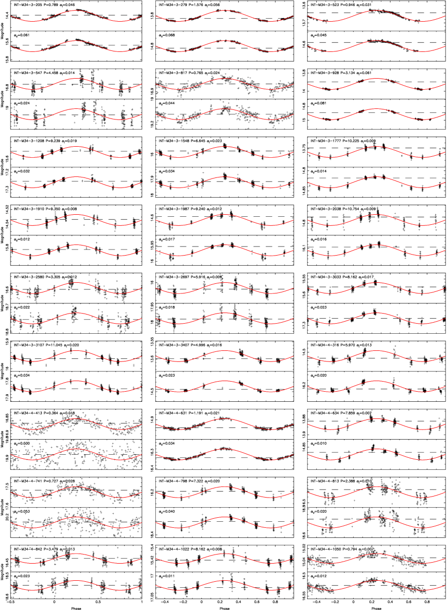
Figure 21: continued

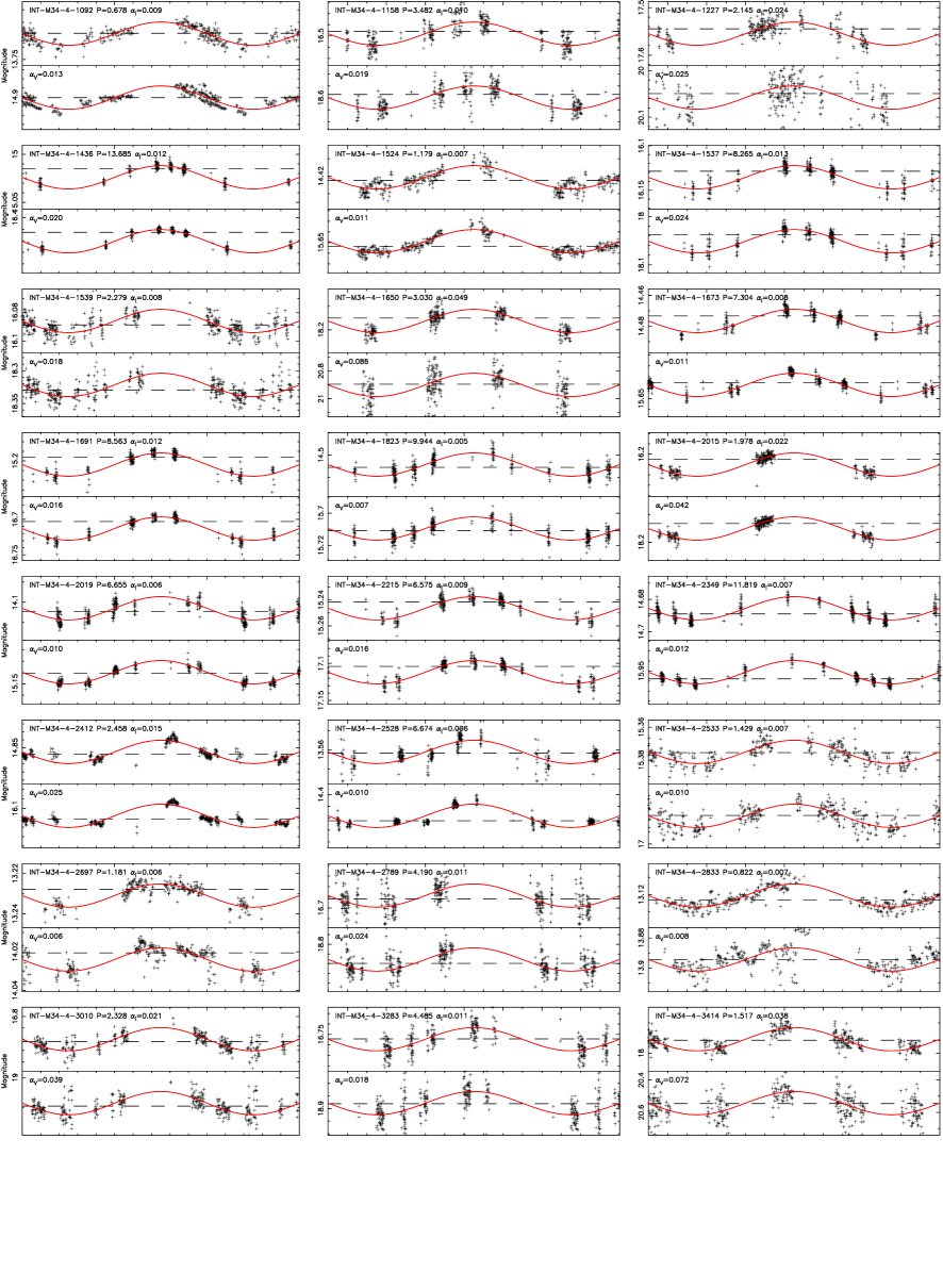
Figure 22: continued

Identifier	RA	Dec	$V$	$R$	$I$	H$\alpha$	$P$	$\alpha_{V}$	$\alpha_{i}$	$M$	$R$	JP	$v\sin i$
	J2000	J2000	mag	mag	mag	mag	days	mag	mag	${\rm M}_{\odot}$	${\rm R}_{\odot}$		${\rm km\ s^{-1}}$
M34-1-304	02 42 56.88	+42 35 22.0	14.52	13.20	13.50	13.91	6.076	0.031	0.024	0.90	0.87	522
M34-1-459	02 42 51.73	+42 33 48.9	17.84	16.74	15.79	16.59	1.444	0.026	0.015	0.58	0.54
M34-1-654	02 42 46.41	+42 39 11.4	15.12	13.90	14.00	14.44	9.356	0.015	0.011	0.82	0.77	487
M34-1-1015	02 42 34.26	+42 31 00.5	18.47	17.34	16.16	17.14	1.105a	0.026	0.016	0.53	0.49
M34-1-1017	02 42 35.02	+42 39 29.0	18.81	17.63	16.46	17.42	3.633	0.052	0.027	0.49	0.45
M34-1-1054	02 42 33.07	+42 30 02.0	18.43	17.28	16.15	17.07	12.311b	0.043	0.026	0.53	0.49
M34-1-1178	02 42 31.54	+42 37 10.5	16.08	15.04	14.58	15.19	1.079	0.042	0.028	0.74	0.69	424	23.3
M34-1-1493	02 42 23.32	+42 38 21.0	17.56	16.48	15.65	16.41	13.500b	0.020	0.012	0.60	0.56
M34-1-1540	02 42 21.89	+42 32 13.1	14.27	12.83	13.20	13.63	6.837	0.017	0.013	0.95	0.92	377	11.1
M34-1-1711	02 42 16.99	+42 38 12.0	18.79	17.59	16.45	17.42	0.929a	0.023	0.012	0.49	0.45
M34-1-1719	02 42 16.16	+42 34 01.0	19.32	18.03	16.72	17.82	0.874	0.048	0.022	0.45	0.41
M34-1-1850	02 42 11.67	+42 31 17.9	17.01	15.95	15.28	15.92	16.812b	0.040	0.028	0.65	0.61
M34-1-1906	02 42 10.65	+42 34 09.1	18.25	17.11	16.09	16.97	2.408	0.033	0.020	0.54	0.50
M34-1-1918	02 42 10.30	+42 34 50.2	16.18	15.13	14.73	15.28	11.389b	0.011	0.007	0.72	0.67
M34-1-1977	02 42 07.85	+42 37 45.1	18.97	17.77	16.55	17.56	1.704	0.033	0.019	0.47	0.43
M34-1-2060	02 42 04.92	+42 37 47.3	17.80	16.69	15.81	16.60	7.778	0.016	0.012	0.58	0.54
M34-1-2324	02 41 55.85	+42 33 32.5	20.26	18.86	17.32	18.62	0.621	0.040	0.022	0.36	0.34
M34-1-2370	02 41 54.69	+42 35 29.7	20.73	19.41	17.88	19.12	0.617	0.039	0.019	0.28	0.28
M34-1-2402	02 41 53.31	+42 32 10.0	19.70	18.49	17.16	18.23	0.349	0.043	0.021	0.38	0.35
M34-1-2414	02 41 53.25	+42 35 26.3	16.48	15.53	14.82	15.49	0.868	0.021	0.011	0.70	0.66
M34-1-2436	02 41 52.59	+42 36 01.6	18.63	17.47	16.36	17.30	7.278	0.025	0.012	0.50	0.46
M34-1-2476	02 41 51.70	+42 38 23.4	16.75	15.85	15.08	15.75	5.082	0.053	0.033	0.67	0.63
M34-1-2483	02 41 51.31	+42 34 24.8	15.06	13.67	13.98	14.40	1.882	0.012	0.007	0.82	0.78	241
M34-1-2573	02 41 48.98	+42 39 59.7	16.18	15.25	14.75	15.31	4.621	0.019	0.011	0.71	0.67
M34-1-2628	02 41 46.37	+42 32 31.9	16.43	15.50	14.93	15.49	7.508	0.009	0.006	0.69	0.65
M34-1-2679	02 41 44.20	+42 35 35.9	17.56	16.48	15.65	16.39	7.349	0.039	0.025	0.60	0.56
M34-1-2694	02 41 43.96	+42 40 31.7	15.68	14.61	14.15	14.73	2.300	0.005	0.006	0.80	0.75	198
M34-1-2813	02 41 39.72	+42 38 06.7	20.70	19.38	17.88	19.09	0.928	0.073	0.044	0.28	0.28
M34-1-2901	02 41 36.60	+42 40 03.9	18.24	17.02	15.87	16.88	5.780	0.020	0.012	0.57	0.53
M34-1-2944	02 41 35.08	+42 33 30.9	14.23	12.80	13.18	13.59	2.509c	0.010	0.006	0.96	0.93	159
M34-1-2953	02 41 35.25	+42 41 02.5	14.63	13.62	13.62	14.05	0.893	0.052	0.038	0.88	0.85	158	45.0
M34-1-3164	02 41 27.66	+42 35 42.1	14.79	13.46	13.85	14.23	6.820	0.007	0.006	0.84	0.80	131
M34-1-3185	02 41 26.29	+42 30 14.9	18.28	17.13	16.13	17.00	2.603	0.033	0.016	0.53	0.49
M34-1-3330	02 41 21.40	+42 35 44.4	15.29	14.03	14.15	14.59	7.689	0.011	0.008	0.80	0.75	105
M34-1-3362	02 41 20.03	+42 39 23.7	18.74	17.56	16.44	17.38	6.614	0.034	0.017	0.49	0.45
M34-2-230	02 40 30.63	+42 51 01.5	14.16	13.24	13.25	13.63	10.759b	0.004	0.004	0.94	0.91
M34-2-548	02 40 09.57	+42 48 37.3	20.37	18.99	17.52	18.76	1.735	0.091	0.045	0.33	0.32
M34-2-599	02 40 49.09	+42 48 20.4	16.69	15.71	15.06	15.69	10.000	0.018	0.015	0.67	0.63
M34-2-742	02 40 15.08	+42 47 13.6	17.88	16.73	15.79	16.62	1.323	0.016	0.012	0.58	0.54
M34-2-774	02 40 24.27	+42 46 57.1	17.82	16.62	15.58	16.52	11.840b	0.016	0.010	0.61	0.57
M34-2-782	02 40 49.66	+42 46 55.0	15.79	15.03	14.47	15.00	6.582	0.045	0.031	0.75	0.70	18
M34-2-948	02 40 26.58	+42 45 40.0	14.16	13.23	13.24	13.61	7.242	0.021	0.015	0.95	0.92
M34-2-1274	02 40 38.20	+42 43 06.6	19.71	18.48	17.08	18.20	1.314	0.046	0.024	0.40	0.36
M34-2-1462	02 40 30.38	+42 41 51.8	14.72	13.61	13.68	14.11	7.177	0.020	0.014	0.87	0.83
M34-2-1659	02 40 26.71	+42 40 15.6	16.62	15.66	14.95	15.60	1.467	0.036	0.022	0.69	0.65
M34-2-1753	02 40 48.54	+42 39 25.7	15.82	14.99	14.49	15.02	0.788	0.031	0.020	0.75	0.70
M34-2-1831	02 40 42.78	+42 38 59.1	16.74	15.74	15.09	15.74	7.033	0.059	0.038	0.67	0.63
M34-2-1834	02 40 05.98	+42 38 57.4	15.22	14.25	14.08	14.51	3.297	0.012	0.008	0.81	0.76
M34-2-2201	02 40 30.81	+42 36 25.0	15.38	14.38	14.21	14.65	3.107	0.009	0.005	0.79	0.74
M34-2-2236	02 40 19.31	+42 36 12.9	16.51	15.56	14.96	15.53	8.790	0.012	0.007	0.69	0.65
M34-2-2471	02 40 57.86	+42 34 39.3	17.30	16.23	15.44	16.17	9.136	0.013	0.009	0.62	0.58
M34-2-2676	02 40 53.92	+42 33 16.5	19.18	17.95	16.54	17.66	0.452	0.035	0.019	0.47	0.43

Table 5: Summary of the properties of our $105$ M34 rotation candidates. The period $P$ in days, and amplitudes $\alpha_{V}$ and $\alpha_{i}$ in the $V$ and $i$ bands (units of magnitudes, in the instrumental bandpass), interpolated mass and radius (from the models of Baraffe et al. 1998, derived using the $I$ magnitudes), identification number of Jones & Prosser (1996), and $v\sin i$ measurements of Soderblom, Jones & Fischer (2001) are given (where available). The following flags are used as superscripts to the period: ‘a’ indicating cases where the period was ambiguous (with both long and short periods fitting equally well to the observations), ‘b’ indicating a poorly-constrained long period (due to the short observing window) and ‘c’ indicating objects where the $V$-band detection was saturated, so the $i$-band only was used to fit the period (NB. the $V$-band magnitudes and amplitudes are unreliable for these objects).

Identifier	RA	Dec	$V$	$R$	$I$	H$\alpha$	$P$	$\alpha_{V}$	$\alpha_{i}$	$M$	$R$	JP	$v\sin i$
	J2000	J2000	mag	mag	mag	mag	days	mag	mag	${\rm M}_{\odot}$	${\rm R}_{\odot}$		${\rm km\ s^{-1}}$
M34-2-2739	02 40 33.29	+42 32 54.3	15.64	14.76	14.38	14.84	8.445a	0.013	0.009	0.76	0.71
M34-2-3071	02 40 48.91	+42 30 34.1	14.60	13.51	13.45	13.88	7.785	0.031	0.020	0.91	0.88
M34-3-205	02 42 59.94	+42 58 01.5	15.81	14.64	14.44	14.94	0.789	0.061	0.046	0.76	0.71	536	44.0
M34-3-279	02 42 57.82	+42 58 03.8	14.97	13.67	13.87	14.25	1.576	0.068	0.056	0.84	0.80	524
M34-3-523	02 42 50.76	+42 58 07.8	14.75	13.58	13.71	14.09	0.946	0.045	0.031	0.86	0.83	499
M34-3-547	02 42 49.81	+43 00 35.3	19.20	17.97	16.72	17.74	4.458	0.024	0.014	0.45	0.41
M34-3-817	02 42 39.42	+42 55 27.7	19.30	18.06	16.78	17.83	0.765	0.044	0.024	0.44	0.40
M34-3-928	02 42 36.30	+42 54 31.4	15.07	13.73	13.98	14.41	3.134	0.081	0.061	0.82	0.78	444
M34-3-1208	02 42 24.90	+42 53 25.9	17.43	16.39	15.55	16.25	9.239	0.032	0.019	0.61	0.57
M34-3-1548	02 42 10.29	+42 59 35.9	18.08	16.90	15.94	16.80	6.645	0.034	0.023	0.56	0.52
M34-3-1777	02 42 02.26	+43 01 13.3	15.01	13.45	13.82	14.25	10.225b	0.014	0.009	0.85	0.81	288	7.0
M34-3-1910	02 41 57.92	+42 53 22.4	15.97	14.71	14.56	15.09	9.350a	0.012	0.008	0.74	0.69	268	7.0
M34-3-1987	02 41 55.95	+42 58 30.8	16.17	14.71	14.69	15.24	9.240a	0.017	0.012	0.72	0.68
M34-3-2038	02 41 54.26	+42 59 35.6	16.29	15.01	14.82	15.36	10.754a	0.016	0.009	0.70	0.66	253
M34-3-2580	02 41 36.18	+42 54 55.7	18.91	17.70	16.52	17.51	3.305	0.022	0.012	0.48	0.44
M34-3-2697	02 41 32.72	+43 02 16.3	18.17	16.98	15.98	16.85	5.916	0.018	0.009	0.55	0.51
M34-3-3033	02 41 18.44	+42 58 21.3	17.45	16.34	15.55	16.27	8.162	0.023	0.017	0.61	0.57
M34-3-3107	02 41 20.45	+42 58 52.3	18.02	16.76	15.95	16.75	11.045b	0.034	0.020	0.56	0.52
M34-3-3407	02 41 05.13	+42 56 43.1	14.65	13.46	13.67	14.00	4.996	0.023	0.016	0.87	0.84	49
M34-4-316	02 42 57.86	+42 41 46.7	16.35	15.22	14.49	15.19	5.970	0.020	0.013	0.75	0.70	527
M34-4-413	02 42 55.14	+42 50 40.8	20.01	18.57	16.69	18.24	0.364	0.030	0.018	0.45	0.41
M34-4-631	02 42 47.53	+42 45 46.8	16.47	15.52	14.94	15.53	1.191	0.034	0.021	0.69	0.65
M34-4-634	02 42 47.72	+42 47 42.9	15.00	13.97	13.94	14.34	7.859	0.010	0.007	0.83	0.79	489	7.8
M34-4-741	02 42 43.65	+42 45 41.8	20.37	19.07	17.38	18.68	0.727	0.053	0.028	0.35	0.33
M34-4-798	02 42 41.81	+42 46 01.8	18.44	17.26	16.12	17.10	7.322	0.040	0.020	0.53	0.49
M34-4-813	02 42 41.06	+42 44 22.2	18.69	17.53	16.42	17.34	2.388	0.020	0.010	0.49	0.45
M34-4-842	02 42 40.62	+42 48 55.6	18.69	17.52	16.37	17.31	3.479	0.023	0.013	0.50	0.46
M34-4-1022	02 42 33.96	+42 43 26.2	17.17	16.08	15.41	16.07	8.162	0.011	0.008	0.63	0.59
M34-4-1050	02 42 33.61	+42 49 12.2	16.66		15.03	15.66	0.794	0.012	0.007	0.68	0.64
M34-4-1092	02 42 32.28	+42 49 05.9	15.05	13.87	13.76	14.25	0.678	0.013	0.009	0.86	0.82	425	17.3
M34-4-1158	02 42 28.95	+42 42 10.5	18.74	17.57	16.42	17.37	3.482	0.019	0.010	0.49	0.45
M34-4-1227	02 42 26.30	+42 43 15.9	20.18	18.88	17.42	18.63	2.145	0.025	0.024	0.34	0.33
M34-4-1436	02 42 20.30	+42 49 05.5	16.57	15.61	15.02	15.60	13.685b	0.020	0.012	0.68	0.64
M34-4-1524	02 42 17.23	+42 48 18.6	15.80	14.95	14.45	14.97	1.179	0.011	0.007	0.75	0.70	356	15.4
M34-4-1537	02 42 16.19	+42 43 11.3	18.17	17.07	16.07	16.92	8.265b	0.024	0.013	0.54	0.50
M34-4-1539	02 42 17.30	+42 51 29.8	18.47	17.25	16.00	17.03	2.279	0.018	0.008	0.55	0.51
M34-4-1650	02 42 12.54	+42 49 28.5	21.00	19.62	18.00	19.35	3.030	0.085	0.049	0.26	0.27
M34-4-1673	02 42 11.71	+42 43 48.2	15.77	14.93	14.51	14.98	7.304	0.011	0.008	0.75	0.70	330
M34-4-1691	02 42 10.99	+42 43 16.3	16.84	15.87	15.18	15.82	8.563	0.016	0.012	0.66	0.62
M34-4-1823	02 42 07.50	+42 47 26.7	15.85		14.53	15.03	9.944	0.007	0.005	0.74	0.69	310
M34-4-2015	02 42 01.81	+42 41 58.9	18.27		16.14	16.99	1.978	0.042	0.022	0.53	0.49
M34-4-2019	02 42 02.55	+42 51 51.4	15.30	14.41	14.17	14.59	6.655	0.010	0.006	0.79	0.74	289	7.4
M34-4-2215	02 41 55.25	+42 50 31.7	17.24	16.14	15.20	16.02	6.575a	0.016	0.009	0.66	0.62
M34-4-2349	02 41 50.31	+42 44 37.6	16.09		14.72	15.22	11.819a	0.012	0.007	0.72	0.67	229	8.2
M34-4-2412	02 41 48.48	+42 49 33.6	16.27	15.41	14.88	15.43	2.458	0.025	0.015	0.70	0.66	218
M34-4-2528	02 41 44.17	+42 46 07.5	14.56		13.62	13.97	6.674	0.010	0.006	0.88	0.85	199	9.5
M34-4-2533	02 41 43.86	+42 45 08.1	17.10	16.13	15.37	16.03	1.429	0.010	0.007	0.63	0.59
M34-4-2697	02 41 38.14	+42 44 04.4	14.15	13.30	13.30	13.64	1.181c	0.006	0.006	0.93	0.90	177
M34-4-2789	02 41 34.88	+42 48 52.7	18.98	17.75	16.62	17.61	4.190a	0.024	0.011	0.46	0.42
M34-4-2833	02 41 33.43	+42 42 11.8	14.04		13.20	13.54	0.822c	0.008	0.007	0.95	0.92	148
M34-4-3010	02 41 26.73	+42 51 34.1	19.24	18.04	16.75	17.81	2.328	0.039	0.021	0.44	0.40
M34-4-3283	02 41 16.53	+42 49 34.8	19.04	17.85	16.67	17.66	4.485	0.018	0.011	0.45	0.41
M34-4-3414	02 41 11.55	+42 46 22.4	20.66	19.37	17.81	19.08	1.517	0.072	0.038	0.29	0.29

Table 6: continued

References

- Allain et al. (1996) Allain S., Fernandez M., Martín E.L., Bouvier J., 1996, A&A, 314, 173
- Allain (1998) Allain S., 1998, A&A, 333, 629
- Baraffe et al. (1998) Baraffe I., Chabrier G., Allard F., Hauschildt P.H., 1998, A&A, 337, 403
- Barnes & Sofia (1996) Barnes S., Sofia S., 1996, ApJ, 462, 746
- Barnes et al. (1998) Barnes J.R., Collier Cameron A., Unruh Y.C., Donati J.F., Hussain G.A.J., 1998, MNRAS, 299, 904
- Barnes et al. (1999) Barnes S.A., Sofia S., Prosser C.F., Stauffer J.R., 1999, ApJ, 516, 263
- Barnes (2003) Barnes S.A., 2003, ApJ, 586, 464
- Barrado y Navascués, Stauffer & Jayawardhana (2004) Barrado y Navascués, D., Stauffer J.R., Jayawardhana R., 2004, ApJ, 614, 386
- Bouvier (1997) Bouvier J., 1997, Mem. S.A.It., 68, 881
- Bouvier et al. (1997) Bouvier J., Forestini M., Allain S., 1997, A&A, 326, 1023
- Canterna, Crawford & Perry (1979) Canterna R., Crawford D.L., Perry C.L., 1979, PASP, 91, 263
- Collier Cameron, Campbell & Quaintrell (1995) Collier Cameron A., Campbell C.G., Quaintrell H., 1995, A&A, 298, 133
- Eff-Darwich, Korzennik & Jiménez-Reyes (2002) Eff-Darwich A., Korzennik S.G., Jiménez-Reyes S.J., 2002, ApJ, 573, 857
- Elias et al. (1982) Elias J.H., Frogel J.A., Matthews K., Neugebauer G., 1982, AJ, 87, 1029
- Elias et al. (1983) Elias J.H., Frogel J.A., Hyland A.R., Jones T.J., 1983, AJ, 88, 1027
- Giampapa et al. (1996) Giampapa M.S., Rosner R., Kashyap V., Fleming T.A., Schmitt J.H.M.M., Bookbinder, J.A., 1996, ApJ, 463, 707
- Haisch, Lada & Lada (2001) Haisch K.E. Jr., Lada E.A., Lada C.J., 2001, ApJ, 553, 153
- Herbst et al. (2002) Herbst W., Bailer-Jones C.A.L., Mundt R., Meisenheimer K., Wackermann R., 2002, A&A, 396, 513
- Hillenbrand (1997) Hillenbrand L., 1997, AJ, 113, 1733
- Hodgkin et al. (2006) Hodgkin S.T., Irwin J.M., Aigrain S., Hebb L., Moraux E., Irwin M.J., 2006, AN, 327, 9
- Ianna & Schlemmer (1993) Ianna P.A., Schlemmer D.M., 1993, AJ, 105, 209
- Irwin & Lewis (2001) Irwin M.J., Lewis J.R., 2001, NewAR, 45, 105
- Jeffries, Thurston & Hambly (2001) Jeffries R.D., Thurston M.R., Hambly N.C., 2001, A&A, 375, 863
- Jones & Prosser (1996) Jones B.F., Prosser C.F., 1996, AJ, 111, 1193
- Kalirai et al. (2003) Kalirai J.S., Fahlman, G.G., Richer H.B., Ventura P., 2003, AJ, 126, 1402
- Keppens, MacGregor & Charbonneau (1995) Keppens R., MacGregor K.B., Charbonneau P., 1995, A&A, 294, 469
- Konacki et al. (2003) Konacki M., Torres G., Jha S., Sasselov, D.D., 2003, Nature, 421, 507
- Königl (1991) Königl A., 1991, ApJ, 370, L37
- Krishnamurthi et al. (1997) Krishnamurthi A., Pinsonneault M.H., Barnes S., Sofia S., 1997, ApJ, 480, 303
- Krishnamurthi et al. (1998) Krishnamurthi et al., 1998, ApJ, 493, 914
- Landolt (1992) Landolt A.J., 1992, AJ, 104, L340
- Leggett (1992) Leggett S.K., 1992, ApJS, 82, 351
- Magnitskii (1987) Magnitskii A.K., 1987, Soviet Astron. Lett., 13, 451
- Martín & Zapatero Osorio (1997) Martín E.L., Zapatero Osorio M.R., 1997, MNRAS, 286, L17
- Meynet, Mermillod & Maeder (1993) Meynet G., Mermillod J.-C., Maeder A., 1993, A&AS, 98, 477
- Moitinho et al. (2001) Moitinho A., Alves J., Huélamo N., Lada C. J., 2001, ApJ, 563, 73
- Moraux et al. (2005) Moraux E., Bouvier J., Clarke C., 2005, Mem. S.A.It., 76, 265
- O’Dell & Collier Cameron (1993) O’Dell M.A., Collier Cameron A., 1993, MNRAS, 262, 521
- O’Dell, Hendry & Collier Cameron (1994) O’Dell M.A., Hendry M.A., and Collier Cameron A., 1994, MNRAS, 268, 181
- O’Dell at al. (1996) O’Dell M.A., Hilditch R.W., Collier Cameron A., Bell S.A., 1996, MNRAS 284, 874
- Patten & Simon (1996) Patten B.M., Simon T., 1996, ApJS, 106, 489
- Perryman et al. (1998) Perryman M.A.C., Brown A.G.A., Lebreton Y., Gomez A., Turon C., de Strobel G.C., Mermilliod J.-C., Robichon N., Kovalevsky J., Crifo F., 1998, A&A, 331, 81
- Prosser (1991) Prosser C.F., 1991, PhD Thesis, University of California, Santa Cruz
- Prosser et al. (1993a) Prosser C.F., Schild R.E., Stauffer J.R., Jones B.F., 1993, PASP 105, 269
- Prosser et al. (1993b) Prosser et al., 1993, PASP, 105, 1407
- Prosser et al. (1995) Prosser et al., 1995, PASP, 107, 211
- Prosser & Randich (1998) Prosser C.F., Randich S., 1998, AN, 319, 210
- Prosser, Randich & Simon (1998) Prosser C.F., Randich S., Simon T. 1998, AN, 319, 215
- Radick et al. (1987) Radick R.R., Thompson D.T., Lockwood G.W., Duncan D.K., Baggett W.E., 1987, ApJ, 321, 459
- Rebull et al. (2006) Rebull L.M., Stauffer J.R., Megeath S.T., Hora J.L., Hartmann L., ApJ accepted (astro-ph/0604104)
- Reid et al. (2002) Reid I.N., Gizis J.E., Hawley S.L., 2002, AJ, 124, 2721
- Robin et al. (2003) Robin A.C., Reylé C., Derrière S., Picaud S., 2003, A&A, 409, 523
- Scholz & Eislöffel (2004) Scholz A., Eislöffel J., 2004, A&A, 421, 259
- Schuler et al. (2003) Schuler S.C., King J.R., Fischer D.A., Soderblom D.R., Jones B.F., 2003, AJ, 125, 2085
- Simon (2000) Simon T., 2000, PASP, 112, 599
- Skumanich (1972) Skumanich A., 1972, ApJ, 171, 565
- Soderblom et al. (1993a) Soderblom D.R., Stauffer J.R., Hudon J.D., Jones B.F., 1993, ApJS, 85, 315
- Soderblom et al. (1993b) Soderblom D.R., Stauffer J.R., MacGregor K.B., Jones B.F., 1993, ApJ, 409, 624
- Soderblom, Jones & Fischer (2001) Soderblom D.R., Jones B.F., Fischer D., 2001, ApJ, 563, 334
- Stassun & Terndrup (2003) Stassun K.G., Terndrup D., 2003, PASP, 115, 505
- Stassun et al. (1999) Stassun K.G., Mathieu R.D., Mazeh T., Vrba F.J., 1999, AJ, 117, 2941
- Stauffer et al. (1985) Stauffer J.R., Hartmann L.W., Burnham J.N., Jones B.F., 1985, ApJ, 289, 247
- Stauffer et al. (1987) Stauffer J.R., Schild R.A., Baliunas S.L., Africano J.L., 1987, PASP, 99, 471
- Stauffer, Hartmann & Jones (1989) Stauffer J.R., Hartmann L.W., Jones B.F., 1989, ApJ, 346, 160
- Stauffer, Schultz & Kirkpatrick (1998) Stauffer J.R., Schultz G., Kirkpatrick J.D., 1998, ApJ, 499, 199
- Stauffer et al. (1999) Stauffer J.R., et al., 1999, ApJ, 527, 219
- Terndrup et al. (1999) Terndrup D.M., Krishnamurthi A., Pinsonneault M.H., Stauffer J.R., 1999, AJ, 118, 1814
- Van Leeuwen, Alphenaar & Meys (1987) Van Leeuwen F., Alphenaar P, Meys J.J.M., 1987, A&AS, 67, 483
- Weber & Davis (1967) Weber E.J., Davis L.Jr., 1967, ApJ, 148, 217