Transverse and longitudinal correlation functions in the Intergalactic Medium from 32 close pairs of high-redshift quasars

Abstract

We present the transverse flux correlation function of the Lyman-$\alpha$ forest in quasar absorption spectra at $z$ $\sim$ 2.1 from VLT-FORS and VLT-UVES observations of a total of 32 pairs of quasars; 26 pairs with separations in the range 0.6 $<$ $\theta$ $<$ 4 arcmin and 6 pairs with 4 $<$ $\theta$ $<$ 10 arcmin. Correlation is detected at the 3 $\sigma$ level up to separations of the order of $\sim$4 arcmin (or $\sim$4.4$h^{-1}$ Mpc comoving at $z=2.1$ for $\Omega_{\rm m}$ = 0.3 and $\Omega_{\Lambda}$ = 0.7). We have, furthermore, measured the longitudinal correlation function at a somewhat higher mean redshift ($z$ = 2.39) from 20 lines of sight observed with high spectral resolution and high signal-to-noise ratio with VLT-UVES. We compare the observed transverse and longitudinal correlation functions to that obtained from numerical simulations and illustrate the effect of spectral resolution, thermal broadening and peculiar motions. The shape and correlation length of the correlation functions are in good agreement with those expected from absorption by the filamentary and sheet-like structures in the photoionized warm intergalactic medium predicted in CDM-like models for structures formation. Using a sample of 139 C iv systems detected along the lines of sight toward the pairs of quasars we also investigate the transverse correlation of metals on the same scales. The observed transverse correlation function of intervening C iv absorption systems is consistent with that of a randomly distributed population of absorbers. This is likely due to the small number of pairs with separation less than 2 arcmin. We detect, however, a significant overdensity of systems in the sightlines towards the quartet Q 0103$-$294A&B, Q 0102$-$2931 and Q 0102$-$293 which extends over the redshift range 1.5 $\leq$ $z$ $\leq$ 2.2 and an angular scale larger than 10 arcmin.

1 Introduction

The numerous H i absorption lines seen in the spectra of distant quasars, the so-called Lyman-$\alpha$ forest, contains precious information on the spatial distribution of neutral hydrogen in the Universe. Unravelling this information from individual spectra has for a long time proven difficult and ambiguous (see Rauch 1998 for a review). Studies of the correlation of the Lyman-$\alpha$ forests observed in the two spectra of QSO pairs have been instrumental in measuring the spatial extent of absorbing structures. The Lyman-$\alpha$ forests in the spectra of multiple images of lensed quasars or pairs of quasars with separations of a few arcsec (Bechtold et al. 1994: Dinshaw et al. 1994; Smette et al. 1995; Impey et al. 1996; Rauch, Sargent & Barlow 1999; Becker, Sargent & Rauch 2004) appear nearly identical implying that the absorbing structures have sizes $>$50$h_{70}^{-1}$ kpc. Significant correlation between absorption spectra of adjacent lines of sight toward quasars still exists for separations of a few to ten arcmin suggesting a size or better a coherence length of the structures larger than 500 $h_{70}^{-1}$ kpc (e.g. Shaver & Robertson 1983; Dinshaw et al. 1997; Petitjean et al. 1998; D’Odorico et al. 1998; Crotts & Fang 1999; Young, Impey & Foltz 2001; Aracil et al. 2002, Rollinde et al. 2003) and a non-spherical geometry of the absorbing structures (Rauch & Haehnelt 1995; Rauch et al. 2005). On even larger scales, Williger et al. (2000) still find evidence for an excess of clustering on 10 Mpc scales.

Numerical simulations of the warm photoionized Intergalactic Medium within the framework of cold dark matter (CDM) like models of structure formation have demonstrated that the neutral gas density traces the underlying dark matter density field on scales larger than the Jeans length of the gas (e.g. Cen et al. 1994; Petitjean, Mücket & Kates 1995; Theuns et al. 1998). The picture of the Lyman-$\alpha$ forest arising from the density fluctuations in a warm photoionized Intergalactic Medium distributed as expected in a CDM model explains the statistical properties of individual QSO absorption spectra very well (see Weinberg et al. 1999 for a review). Most of the baryons are located in filaments and sheets which are only overdense by factors of a few and produce absorption in the column density range 10¹⁴ $<$ $N_{\rm HI}$ $<$ 10¹⁵ cm^-2 at $z\sim 2$. On the other hand, most of the volume is occupied by underdense regions that produce absorption with $N_{\rm HI}<10^{14}$ cm^-2. Analytical calculations and numerical simulations of the spatial distribution of neutral hydrogen in $\Lambda$CDM models are also able to reproduce the large observed transverse correlation length of the Lyman-$\alpha$ forest in the absorption spectra of QSO pairs (Bi 1993; Miralda-Escudé et al. 1996; Charlton et al. 1997; Viel et al. 2002; Rollinde et al. 2003; Rauch et al. 2005).

As pointed out by several authors a comparison of the transverse correlation to the correlation observed along the line of sight, can be used to carry out a variant of the Alcock & Paczyński (1979) test to put constraints on the geometry of the Universe (Hui, Stebbins & Burleset 1999; Mc Donald & Miralda-Escudé 1999; Mc Donald 2003). This provides strong motivation for an (accurate) measurement of the transverse correlation function.

In a previous work we have used 5 pairs and a group of 10 quasars with separations in the range 1-10 arcmin to investigate whether the longitudinal and transverse correlation functions were consistent with those expected in $\Lambda$CDM models (Rollinde et al. 2003). We reported a somewhat marginal detection of a transverse correlation up to separations of 3 to 4 arcmin. We have assembled here a significantly larger sample of 32 QSO pairs. The new sample consists of 26 pairs with separations in the range 0.6$-$4 arcmin (corresponding to $\simeq$ 0.2 to 1.4 $h^{-1}$ Mpc proper at z=2.1 for $\Omega_{\rm m}=0.3$, $\Omega_{\Lambda}=0.7$) and 6 pairs with separations in the range 5$-$10 arcmin.

Details of the observations and simulations are given in Sections 2 and 3, respectively. In Section 4 we define and discuss our measurements of the observed longitudinal and transverse flux correlation functions. Section 5 compares the observed and simulated correlation functions. We investigate the transverse correlation of C iv absorption systems in Section 6. Our conclusions are given in Section 7. Comments on individual lines of sight are given in Appendix A. Metal-line lists and QSO spectra are given in Appendix B and C available in the electronic version of the paper.

2 Observations

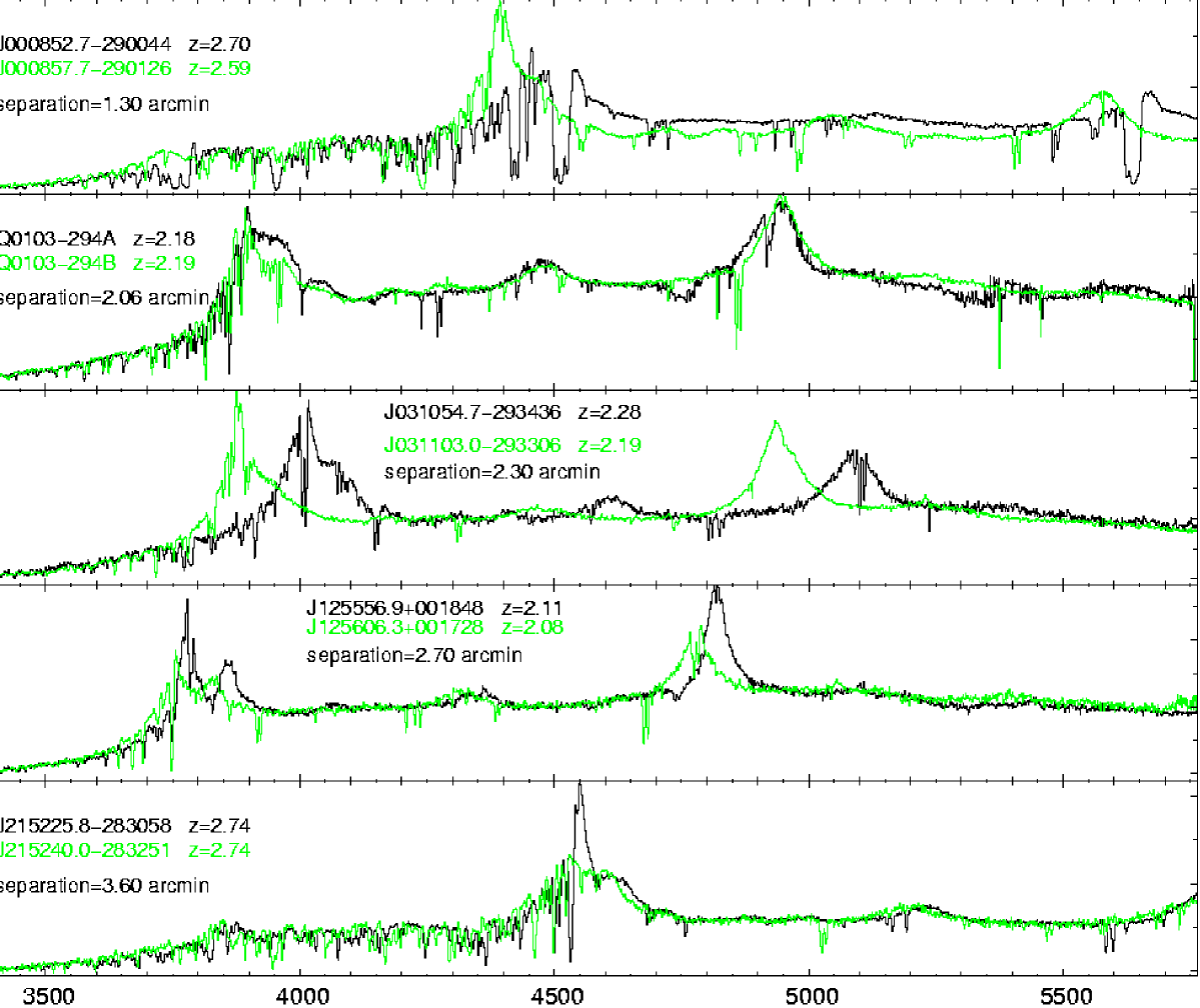
Figure 1: Typical observed spectra of QSO pairs in order of increasing right ascension. QSO names, emission redshifts and angular separations are given in the top-left corner of each sub-panel. Other spectra are presented in Appendix C published in the electronic version of the paper.

The first release of the 2dF quasar survey has significantly enlarged the number of known quasar pairs with arcmin separation (Outram, Hoyle & Shanks 2001). We have selected pairs with the following criteria to enlarge the number of small separation pairs with respect to the sample of Rollinde et al. (2003): (i) the separation of the two quasars should be in the range 1$-$4 arcmin where the correlation is expected and observed to be strong; (ii) the quasars should be brighter than $m_{\rm V}$ = 20.30 to keep observing time in reasonable limits; (iii) the emission redshifts of the two quasars should be larger than $z$ $\sim$ 2.1 to increase the wavelength range over which high S/N ratio can be obtained (FORS is not sufficiently sensitive below 3500 Å); (iv) the redshift difference should be smaller than $\Delta z$ $\sim$ 0.5 (for most of them 0.3) to maximise the wavelength range over which correlation can be studied.

There are 22 quasar pairs in the 2dF survey which meet our criteria of which we observed 20. We have observed two additional pairs not contained in 2dF : J 123510.5-010746$-$J 123511.0-010830 with a separation of 0.74 arcmin and Q 1207-1057$-$Q 1206-1056 with a separation of 3.5 arcmin. The spectra were obtained with FORS1 and 2 mounted on the VLT-UT2 and UT3 telescopes of ESO using the grism GR630B and a 0.7 arcsec slit. The spectra were reduced using standard procedures available in the context LONG of the ESO data reduction package MIDAS. Master bias and flat-fields were produced using day-time calibrations. Bias subtraction and flat-field division were performed on science and calibration images. A correction for 2D distortion was applied. The sky level was evaluated in two windows on both sides of the object offset along the slit direction and subtracted on the fly during the optimal extraction of the object. The spectra were then wavelength calibrated over the range 3400 $<$ $\lambda$ $<$ 6000 Å. The final pixel size is 1.18 Å  corresponding to a resolution of $R$ = 1400 or FWHM = 220 km s^-1 at 3800 Å. The exposure times have been adjusted in order to obtain a typical signal-to-noise ratio of $\sim$10 at 3500 Å. The sharp decrease of the detector sensitivity below 4000 Å  prevents scientific analysis below $\sim$3500 Å. At $\lambda$ $\sim$ 4500 Å  the S/N ratio is usually larger than 70. The final sample consists of 58 QSOs (44 QSOs new from this program, 12 QSOs from Rollinde et al. 2003 plus the pair UM680-UM681 presented in D’Odorico et al. 2002). The total number of pairs included in our analysis of the transverse correlation function is 32 somewhat larger than half the total number of QSOs due to the additional pairings of Q 0103$-$294A&B, Q 0102$-$2931 and Q 0102$-$293 which form a group (alternative names are, respectively, J010534.7-290917, J010538.3-291106, J010518.0-291510 and J010502.8-290618). One further pair in the sample (J 123510.5-010746$-$J 123511.0-010830) was at the end not included in our analysis of the transverse correlation function as the redshift overlap of the Lyman-$\alpha$ forest is too small to contribute in a statistically significant way.

Table 1 gives a summary of the sample including emission redshifts, angular separation of the pairs on the sky, the mean S/N ratio in the wavelength range of interest. Emission redshifts were determined by fitting a Gaussian function to the Civ emission line when present in the spectrum or to the Lyman-$\alpha$ emission line otherwise. Typical spectra are shown in Fig  1. Other spectra are presented in Appendix C published in the electronic version of the paper.

The spectra have been normalized using a spline fit to the continuum. This operation is important as it can affect the estimate of the mean flux which is in turn critical for the flux correlation function estimate. In our sample most of the Lyman-$\alpha$ forest common to two QSOs lies at $z$ $<$ 2.3. At this redshift the density of absorption features is moderate and there are numerous spectral regions with no absorption. This is why continuum fitting is reliable. For the same reason, the identification of metal absorption systems in the Lyman-$\alpha$ forest region of the spectrum is unproblematic. We have checked that the mean absorption of the spectra in our sample is consistent with that measured from the data of the VLT Large Program (LP) ’The Cosmic Evolution of the IGM’ (Aracil et al. 2004, 2006 and below).

To calculate the longitudinal correlation function we also use the data from the LP ’The Cosmic Evolution of the IGM’ which has produced a sample of absorption spectra of homogeneous quality suitable for studying the Lyman-$\alpha$ forest in the redshift range 1.7$-$4.5. The spectra of the LP have been taken with VLT-UVES and have high resolution ($R$ $\sim$ 45000), high signal to noise ratio (30 and 60 per pixel at respectively 3500 and 6000 Å) and cover the wavelength ranges 3100–5400 and 5450–9000 Å. Details of the data reduction and normalization of the spectra are given in Aracil et al. (2004, 2006).

3 Numerical simulations

In this paper we use two numerical simulations to estimate the errors and the effect of numerical resolution, redshift distortion and the thermal state of the gas on the correlation functions: a large size dark-matter only simulation and a smaller size full hydrodynamical simulation. For both simulations we assume parameters consistent with the fiducial concordance cosmological model $\Omega_{\Lambda}=0.7$, $\Omega_{\rm m}=0.3$. Hubble constants are $h=0.65$ and $h=0.7$ and normalization of the fluctuation amplitude of the matter power spectrum are $\sigma_{8}=0.93$ and $\sigma_{8}=1.0$ for the dark-matter only and the full hydrodynamical simulation, respectively. The assumed baryon density in the hydro-dynamical simulations is $\Omega_{\rm b}$ = 0.04. The simulations were performed on the computers of the Institut du Developpement et des Ressources en Informatique Scientifique (IDRIS) in Orsay.

The hydro-dynamical simulation of 40 Mpc box-size and dark-matter only simulation of 100 $h^{-1}$Mpc  box-size are used to catch both the statistical aspects and the effect of gas physics. In the hydro-simulation some weak bias on the correlation functions due to the box-size is expected at separation larger than 4 Mpc. However, larger hydrodynamical simulations that still resolve the Jeans length at least marginally are currently not feasible.

The dark-matter only simulation was performed with the Particle - Mesh (PM) code described in Pichon et al. (2001) and was also used in Rollinde et al. (2003). The simulation has 16 million particles and a box-size of 100 $h^{-1}$Mpc. The large box-size ensures a sufficient statistical sampling on large scales where thermal effects and pressure effects which are modelled approximately in the dark-matter only simulation are less important. Initial conditions were set up using a standard CDM transfer function (Efstathiou, Bond & White 1992). To construct mock Lyman-$\alpha$ spectra from the simulated data, we proceed as in Rollinde et al. (2001, 2003) applying simple semi-analytical prescriptions taking into account thermal broadening and redshift distortion. The density and velocity fields are interpolated on a 256³ grid. We use adaptive smoothing similar to SPH smoothing but with a Gaussian window truncated at $3\sigma$, as explained and tested in Pichon et al. (2001). This eliminates discreteness effects while keeping the best spatial resolution possible. The pixel size of the dark-matter only simulation is 0.4 $h^{-1}$Mpc. This corresponds to 0.47 Å, a factor 2.5 smaller than the pixel size of the FORS spectra. We have convolved the mock spectra from the numerical simulations with a Gaussian filter to match the spectral resolution of the observed spectra.

The hydrodynamical simulation is better suited for investigating the effects of thermal broadening and redshift distortions which are more relevant on small scales. This simulation has 512³ dark matter particles and follows the gas dynamics on a fixed cubic grid with 512³ cells. The simulation has a box-size of 40 Mpc; the mesh size is $\sim$ 80 $h^{-1}$kpc which corresponds to a pixel size of 0.07 Å  at a redshift $z=2$. This means that the Jeans length of the warm photo-ionized IGM is marginally resolved. We have used simulations with box-size of 20 and 10 Mpc to check that the 40 Mpc simulation used here is not significantly affected by the fact the Jeans mass is only marginally resolved. The 40 Mpc size therefore offers the best compromise between box-size and resolution and the statistical properties of the absorption spectra studied here are sufficiently converged. The dark matter distribution is modelled with the same PM code as the dark-matter only simulation. The hydrodynamical part of the code is the same as in Chièze, Alimi & Teyssier (1998) and Teyssier, Chièze & Alimi (1998). The adiabatic hydrodynamic step is solved using directional splitting and a staggered mesh. Shock waves are approximated with the pseudoviscosity method (Von Neuman & Richmyer 1950). An additional dissipative step models the physical processes relevant for the description of gas dynamics in a photoionized intergalactic medium, as described in the Appendix B of Theuns et al. (1998), except that we use the heating and photoionization rates of Davé et al. (1999) which were derived from measurements by Haardt & Madau (1996). The Intergalactic Medium is highly ionized at the relevant redshifts and the dynamical evolution of the gas in the simulation depends therefore only very weakly on the amplitude of the ionizing flux characterized by its value at the Lyman limit: $J_{21}$. We have run the simulation with the same ionizing flux as adopted in Davé et al. (1999). However, when we are producing mock spectra, we compute the equilibrium ionic abundances in a post-processing step for a rescaled ionizing flux such as to match the observed flux distribution (see section 5.1). This procedure does not affect the density and temperature distribution of the gas, as specified in Theuns et al. (1998).

4 The observed longitudinal and transverse correlation functions

4.1 Calculating correlation functions

We define the flux correlation function as in Rollinde et al. (2003):

$$\xi_{f}(\theta,\Delta v)=\left\langle({\cal F}(\theta,\lambda+\Delta\lambda)-\langle{\cal F}\rangle)({\cal F}(0,\lambda)-\langle{\cal F}\rangle)\right\rangle_{\lambda}\,,$$ (1)

where ${\cal F}$ is the normalized flux along two lines of sight with separation $\theta$ at a mean redshift $z$; $\Delta\lambda=\lambda_{0}(1+z)\times\Delta v/c$, with $\lambda_{0}=1215.67$ Å  the hydrogen Lyman-$\alpha$ rest-wavelength, and $c$ denotes the speed of light. The velocity distance corresponding to the angular separation $\theta$ can be written as $\Delta v_{\perp}=c\,f(z)\,\theta$, where $f(z)=c^{-1}H(z)D_{A}(z)$, $H(z)$ is the Hubble constant at $z$, and $D_{A}(z)$ is the angular diameter distance (see Mc Donald 2003). For $\theta=0$ equation (1) gives the longitudinal correlation function. In the following we will use $H_{\rm 0}$ = 70 km/s/Mpc, $\Omega_{\rm m}$ = 0.3, $\Omega_{\Lambda}$ = 0.7 to relate scales in redshift space with angular scales. With these parameters $\Delta v$ = 100 km s^-1 corresponds to $\sim$1 arcmin at $z$ = 2.

We have excluded the wavelength range less than 1000  km s^-1 redward of the Lyman-$\beta$ emission line when calculating the observed correlation functions to avoid contamination from the Lyman-$\beta$ forest. Likewise spectral regions less than 3000  km s^-1 blueward of the Lyman-$\alpha$ emission line have been excluded to avoid the proximity effect (see Rollinde et al. 2005). Damped absorption systems and metal lines which we were able to identify have been removed. The properties of identified damped absorption systems are listed in Table 3 and the properties of the metal lines are listed in the Appendix B published in the electronic version of the paper.

4.2 The observed longitudinal correlation function

The observed correlation functions depend strongly on the spectral resolution of the absorption spectra unless the width of all spectral features is fully resolved (e.g Becker, Sargent & Rauch 2004).

We first consider the longitudinal correlation function obtained from the FORS data. The thick dashed line in Fig. 2 shows the average of the longitudinal correlation functions measured from the 58 FORS spectra in the sample. Errors are calculated from the variance of the measurements (see Section 4.4).

The longitudinal correlation function measured from the high resolution spectra obtained in the course of the UVES-VLT LP is shown as a thick solid curve in Fig. 2. The high-resolution spectra have a mean redshift of 2.39. As expected, the correlation function of the high-resolution spectra extends to higher values at small velocity separation. We also show the longitudinal correlation function obtained by Mc Donald et al. (2000) from a smaller sample of eight high-resolution spectra with a mean redshift of $z$ = 2.41 obtained with Keck-HIRES as the thin solid curve. There is excellent agreement for the two samples of high-resolution spectra at velocity separations $\leq$ 300 km s^-1. At velocity separations of $\sim$ 400 km s^-1, the longitudinal correlation function obtained from the UVES spectra appears to be larger than that obtained from the HIRES spectra. Cosmic variance or artefacts due to continuum fitting errors are two plausible explanations. Note, however, that the errors are already rather large at these separations and that the difference is probably not statistically significant.

The thin dotted curve shows the longitudinal correlation from the high-resolution VLT-UVES spectra after convolution with a Gaussian filter of FWHM = 220 km s^-1 to take into account the difference in resolution of the UVES and FORS spectra. It agrees very well with the FORS correlation function up to a small systematic offset.

\begin{picture}(9.0,8.0)\centerline{\hbox{\psfig{width=213.39566pt}}} \end{picture}

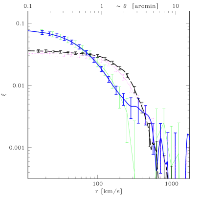
Figure 2: The observed longitudinal correlation functions derived from low resolution FORS spectra (thick dashed curve), high-resolution VLT-UVES (thick solid curve) and high resolution KECK-HIRES spectra (Mc Donald et al. 2000, thin solid curve). The thin dotted curve shows the correlation function from the VLT-UVES spectra after convolution of the spectra with a Gaussian filter of FWHM = 220 km s^-1 to match the resolution of the FORS spectra. Errors for the FORS and UVES spectra have been estimated from the observations as described in the text.

4.3 The observed transverse correlation function

\begin{picture}(9.0,8.0)\centerline{\hbox{\psfig{width=213.39566pt}}} \end{picture}

Figure 3: The observed transverse correlation coefficient for individual pairs (black triangles, dashed error bars; see Table 1) and a binned estimate of the transverse correlation function (solid error bars). The error bars for the individual measurements are estimated using the dark-matter only simulation as explained in Section 4.4

The correlation function is calculated using the 32 pairs presented in Table 1. We use only spectral regions where the S/N ratio in both spectra is larger than 8. For this reason the pair J 123510.5-010746$-$J 123511.0-010830 is not included in the analysis as the redshift overlap of the two Lyman-$\alpha$ forests is too small to contribute in a statistically significant way. The wavelength range ($\lambda_{\rm max}-\lambda_{\rm min}$) used to compute the transverse correlations is given in Table 1 together with the corresponding number of pixels. The mean flux is taken over each individual line of sight.

In Fig. 3 we show the observed transverse correlation function. The measurement for each quasar pair, $\chi(\theta_{\rm i})\equiv\xi_{f}(\theta_{\rm i},\Delta v=0)$, is shown as a small solid triangle at the angular separation of the pair, $\theta_{\rm i}$. The points with the solid error bars are a binned estimate of the transverse correlation function for which we have weighted the individual measurements with the inverse of their errors (see Section 4.4 for the computation of errors). Note that the first bin at the smallest separation contains only one measurement.

The transverse correlation is clearly detected on scales $<4$ arcmin. If we merge the two bins between 3 and 4 arcmin, the correlation is detected at about the 3$\sigma$ level.

Note that correlation coefficients derived from this work for some of the pairs observed by Rollinde et al. (2003) differ somewhat from what is given in their paper (see Table 1). This is due to slight differences in the reduction of the data and the determination of the continuum.

4.4 Estimation of errors

The measurements of the longitudinal correlation reported in Fig. 2 are the average of the correlation function of the individual spectra $\xi_{i}(\Delta v)$ (58 spectra in the case of FORS and 20 in the case of UVES),

$${\bar{\xi}}(\Delta v)=\frac{1}{N}\sum_{i=1}^{N}\xi_{i}(\Delta v)\,.$$ (2)

The error of the mean correlation function is then computed as, $(\Delta\xi)^{2}\simeq 1/N(N-1)\sum_{i=1}^{N}[\xi_{i}-{\bar{\xi}}]^{2}.$ For the transverse correlation there is only one measurement (one pair) at each separation. We therefore use the dark matter-only simulation to estimate the statistical errors. We choose samples of random sightlines along one axis of the box carefully reproducing individual pair separations, wavelength coverage, resolution and the noise of the spectra in the observed sample. The length of the observed spectra is always larger than 100 $h^{-1}$Mpc, and we have concatenated several lines of sight through the simulation box in order to reproduce one observed spectrum. Note that we use only one output of the simulation at $z=2$ and did not try to account for the moderate redshift evolution in our sample. We extract 10000 different realizations from the simulation. We then fit a Gaussian to the distribution of the values of the correlation function at each separation ${\hat{\xi}}_{j}$ and use the rms of the distribution as estimate for the error of the transverse correlation function as reported in Table 1 and Figure 3.

Note that the errors quoted here on the flux correlation functions are only indicative because they are strongly correlated (see McDonald et al. 2000).

5 Comparison of observed and simulated correlation functions

5.1 Numerical simulations as a testbed for systematic uncertainties

The longitudinal and transverse correlation functions reflect the clustering of the underlying matter distribution in real space albeit in a somewhat indirect way. The correlation functions calculated from mock spectra produced from numerical simulations are an excellent tool to test the effects of resolution, redshift space distortion, thermal broadening and non-linear evolution of the gravitational clustering. We use here the 512³ cell full hydro-simulation described in Section 3. When thermal broadening and redshift-distortion are taken into account, they are computed from the temperature and velocity fields of the simulation as described in Theuns et al. (1998). We produce spectra for all lines of sight along one axis of the simulation box separated by one cell. This corresponds to 512² sightlines with a length of 512 pixels each. Our estimate of the longitudinal correlation function from the simulations is obtained by averaging over these 512² individual realisations. The transverse correlation function is computed at 20 log-spaced values of $\theta$. We average over pairs of lines of sight for each value of $\theta$ in the following way. For each of the $512^{2}$ pixels in the y-z plane, we take the sightline parallel to the x-axis as the first spectrum of a pair. We then use two parallel lines of sight separated by a distance $\theta$, in the y-direction and z-direction, respectively, to compute the second spectrum to obtain two pairs of spectra. Our estimate of the transverse correlation is the average of the resulting $2\times 512^{2}$ pairs.

The normalization of the correlation function depends sensitively on the mean flux which in turn depends on the amplitude of the ionizing flux. Therefore, the mock spectra were calculated with a rescaled ionizing flux such that the probability distribution function (PDF) of the flux distribution matches that of our observed spectra at the same redshift for $\tau$ = 1. We proceed iteratively starting with an arbitrary ionizing flux and adjusting this flux step by step till the fit is obtained. We found that this procedure is similar although more robust than the conventional procedure to match the mean flux in the Lyman-$\alpha$ forest. Indeed, the fit of the PDF minimizes the role played by overdensities and the effect of cosmic variance.

Figure 4: The longitudinal and transverse correlation functions versus velocity separation (lower x-axis) and angular separation (upper x-axis) for the full hydro-simulation at $z$ = 2. Upper panel: the longitudinal correlation of the gas density (thick dotted curve) is nearly identical to the transverse correlation at the same redshift (thin dotted curve) as expected. The correlation functions differ when thermal broadening (longitudinal: thick dashed curve, transverse: thin dashed curve) and peculiar velocities (longitudinal: thick solid curve, transverse: thin solid curve) are taken into account. Lower panel: Ratio of the longitudinal and transverse correlation functions. Linestyles are the same as in the upper panel.

The thick and thin dotted curves in Fig. 4 show, respectively, the longitudinal and transverse correlation functions in real space as calculated from mock spectra produced from the full hydro-simulation. We have again used our fiducial cosmological parameters to relate velocity and angular separation. As expected the two correlation functions are almost identical. The dashed curves show the same comparison with the effect of thermal broadening included. There are now significant differences. At small scales the longitudinal correlation function exceeds the transverse correlation function while at large scales the opposite is true. The solid curves show the effect of including peculiar velocities. The corresponding redshift distortion further enhances the differences between longitudinal and transverse correlation functions. The scale dependence of the difference is similar to that due to thermal broadening but the differences are significantly larger especially at scales larger than 200 km s^-1 or 2 arcmin.

A proper quantitative understanding of these effects with the help of numerical simulations will be essential for attempts to use the comparison of observed longitudinal and transverse correlation functions to measure cosmological parameters. This would need a full set of simulations spanning the whole range of parameters and is therefore beyond the scope of this paper.

5.2 Observed vs simulated correlation functions

\begin{picture}(9.0,8.0)\centerline{\hbox{\psfig{width=213.39566pt}}} \end{picture}

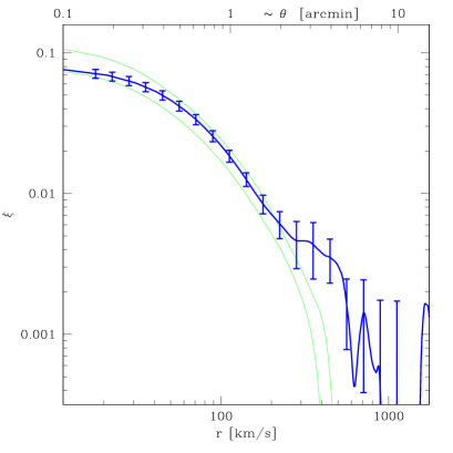
Figure 5: The observed longitudinal correlation function from the high resolution UVES spectra (thick solid curve) compared to the longitudinal correlation function as measured in the full hydro-dynamical simulation at $z=2$ (lower thin curve) and $z=3$ (upper thin curve), respectively.

The ability of $\Lambda$CDM models to reproduce the longitudinal correlation function of the Lyman-$\alpha$ forest has been demonstrated by many authors (e.g. Croft et al. 2002, Viel et al. 2002, Rollinde et al. 2003) and, as we will see below, the same is true for our simulations. The thin solid curves in Fig. 5 show the mean longitudinal correlation function obtained for mock spectra produced from the hydrodynamical simulation at $z=2$ (lower curve) and $z=3$ (upper curve). The curves nicely bracket the observed correlation function obtained from the high-resolution data with a median redshift of $z=2.39$. Note again the slight excess of the longitudinal correlation function of the UVES data at large scales which is, however, probably not statistically significant.

\begin{picture}(9.0,8.0)\centerline{\hbox{\psfig{width=213.39566pt}}} \end{picture}

Figure 6: The binned estimate of the observed transverse correlation function (solid error bars) is shown together with the estimate of the transverse correlation function from the full hydro-simulation (thick solid curve) and linear predictions for $\Omega_{\rm m}$ = 0.1, 0.3 and 1 (thin solid, dashed and dotted lines respectively, assuming a flat universe : $\Omega_{\Lambda}+\Omega_{m}=1$; see text). The normalization of the flux in the simulation is fixed in order to reproduce the observed flux PDF (Section 5.2). The linear theory predictions are normalized to reproduce the longitudinal correlation function at large scales.

The transverse correlation contains precious direct information on the physical size/coherence-length of the absorbing structures as it is less affected by redshift space distortions than the longitudinal correlation function. Furthermore, a comparison of the longitudinal and transverse correlation functions can – at least in principle – strongly constrain cosmological parameters in particular $\Omega_{\Lambda}$.

The thick solid curve in Figure 6 shows our estimate of the transverse correlation function from the full hydro-dynamical simulation at $z=2$. It agrees well with our measurement of the observed transverse correlation function (mean redshift $\sim$2.1) which is shown as the solid dots with error bars. The thin dashed curve shows the prediction of linear theory (Kaiser 1987; Mc Donald & Miralda-Escudé 1999) for the cosmological parameters assumed for the hydro-simulation. The thin solid and dotted curves show the prediction of linear theory for $\Omega_{\rm m}=0.1$ and $\Omega_{\rm m}=1.0$, respectively (assuming a flat universe : $\Omega_{\Lambda}+\Omega_{m}=1$ and adjusting other parameters to fit the data). The linear theory predictions are normalized so that the longitudinal correlation function is best fitted for $\Delta v>200$ km s^-1. As expected, the linear predictions agree reasonably well with the numerical simulation at large scales but underpredicts the correlation function substantially at small scales. The non-linear effects of gravitational clustering are clearly visible in the observed transverse correlation function.

Despite the larger sample (about three times more pairs at $\theta<3$ arcmin than in Rollinde et al. 2003) and the correspondingly smaller errors, we cannot yet distinguish between different values of $\Omega_{\rm m}$. This confirms the predictions by Rollinde et al. (2003) and Mc Donald (2003) that significant constraints on $\Omega_{\Lambda}$ require a larger number of pairs. Using the (cross) power spectrum instead of the transverse and longitudinal correlation functions, Mc Donald (2003) estimates that of the order of 13($\theta$/1’)² quasar pairs on scales up to 10 arcmin are necessary to perform the test. In addition, performing the Alcock & Paczyński test using the correlation functions at small scales ($\leq$ 3 arcmin or 300 km s^-1 at $z$ = 2) will require the use of a large suite of full hydro-dynamical simulations.

QSO name	$z_{\rm em}$	$\Delta\theta$	SNR	$\lambda$	Number	$\xi(0,\theta)$	$\sigma$
		(arcmin)		(Å)	of pixels
$*$Q2139-4504B	3.255	0.600	24.4	4381- 4878	420	0.025	0.009
Q2139-4504A	3.055		15.2
J 123510.5-010746	2.785	0.740	51.4	3897- 3904	7	-	-
J 123511.0-010830	2.235		26.2
J 232800.7-271655	2.378	0.900	14.3	3756- 4038	240	0.016	0.010
J 232804.4-271713	2.357		14.3
UM680	2.144	1.000	50.0	3235- 3699	9641a	0.011	0.008
UM681	2.122		50.0
J 031036.4-305108	2.552	1.200	20.9	3658- 4249	501	0.018	0.007
J 031041.0-305027	2.532		25.4
J 135001.7-011703	2.657	1.300	15.5	3765- 3821	48	0.018	0.019
J 135003.0-011819	2.177		18.5
J 000852.7-290044	2.699	1.300	64.1	3808- 4323	317	0.008	0.007
J 000857.7-290126	2.593		34.2
J 214507.0-303046	2.532	1.300	37.5	3636- 3869	177	0.003	0.011
J 214501.6-303121	2.216		27.3
J 005852.4-272933	2.565	1.800	23.9	3671- 4284	493	0.008	0.006
J 005859.1-273038	2.561		25.5
$*$Q0103-294B	2.190	2.063	25.5	3602- 3827	191	0.012	0.008
Q0103-294A	2.182		28.3
$*$Q2129-4653B	2.222	2.100	22.4	3603- 3856	215	0.004	0.008
Q2129-4653A	2.206		16.8
J 031054.7-293436	2.281	2.300	18.3	3601- 3833	197	0.006	0.007
J 031103.0-293306	2.187		29.3
J 102827.1-013641	2.393	2.300	13.4	3728- 3954	193	0.018	0.007
J 102832.6-013448	2.287		17.0
J 111201.8-013018	2.549	2.400	48.7	3654- 3954	246	0.014	0.006
J 111200.4-013242	2.292		28.1
$*$Q0236-2411	2.260	2.600	20.3	3602- 3860	219	0.009	0.007
Q0236-2413	2.211		19.4
J 125556.9+001848	2.108	2.700	19.9	3602- 3708	90	0.004	0.010
J 125606.3+001728	2.083		20.0
J 013734.2-303802	2.481	2.800	24.4	3602- 4005	341	0.005	0.005
J 013734.2-304050	2.329		29.2
J120725.9-024519	2.676	3.000	33.2	3785- 3904	101	0.007	0.009
J120734.5-024725	2.245		20.0
J 095810.9-002733	2.559	3.000	21.4	3664- 4047	287	0.002	0.006
J 095800.2-002858	2.364		14.2
J 223850.1-295612	2.448	3.180	32.0	3602- 4062	390	0.003	0.005
J 223850.9-295301	2.377		34.2
J 141124.6-022943	2.710	3.210	43.2	3820- 3971	128	0.008	0.008
J 141117.3-023222	2.301		35.3
J 023836.9-282310	2.565	3.400	31.7	3677- 3899	175	0.006	0.007
J 023849.0-282101	2.242		56.7
Q 1207-1057	2.450	3.500	33.8	3601- 3975	318	0.006	0.005
Q 1206-1056	2.305		24.7
J 215225.8-283058	2.741	3.600	38.0	3851- 4494	545	0.002	0.004
J 215240.0-283251	2.736		25.3
J 112116.1+003112	2.205	3.700	19.0	3603- 3834	197	0.001	0.006
J 112108.2+003420	2.188		22.8
J144245.7-023906	2.551	3.740	24.3	3656- 4011	232	0.006	0.006
J144245.6-024251	2.334		21.2
J 230318.4-290120	2.587	3.800	35.5	3693- 4285	500	0.003	0.004
J 230301.6-290027	2.562		26.9

Table 1: Properties of the 33 QSO pairs: QSO names, emission redshifts, angular separation on the sky, mean S/N ratio over the wavelength range of interest, wavelength range (in Å) over which the correlation is calculated, corresponding number of pixels, value of the correlation function and errors (see Section 4.4). (a) UVES data (D’Odorico et al. 2002) with 0.04 Å  per pixel instead of 1.18 Å  for FORS data. (*) QSO pair observed by Rollinde et al. (2003).

QSO name	$z_{\rm em}$	$\theta$	SNR	$\Delta\lambda$	Number	$\xi(0,\theta)$	$\sigma$
		(arcmin)		(Å)	of pixels
$*$FOCAP QSF:01	2.267	4.400	21.5	3602- 3673	61	0.000	0.010
FOCAP QSF:04	2.054		19.0
$*$Q0102-2931	2.212	5.974	18.5	3603- 3837	199	0.011	0.006
Q0103-294B	2.190		25.5
$*$Q0102-2931	2.212	6.977	18.5	3602- 3827	191	0.006	0.006
Q0103-294A	2.182		28.3
$*$Q0102-293	2.441	7.585	24.8	3602- 3827	191	0.002	0.006
Q0103-294A	2.182		28.3
$*$Q0102-293	2.441	9.152	24.8	3603- 3837	199	-0.003	0.006
Q0103-294B	2.190		25.5
$*$Q0102-293	2.441	9.506	24.8	3602- 3864	222	-0.003	0.008
Q0102-2931	2.212		18.5

Table 2: continued

- Alternative names for FOCAP QSF:01 and FOCAP QSF:04 are J034105.1-445619 and J034126.2-445842.

6 Metal absorption systems

\begin{picture}(9.0,10.0)\centerline{\hbox{\psfig{height=298.75394pt,width=241.84842pt}}} \end{picture}

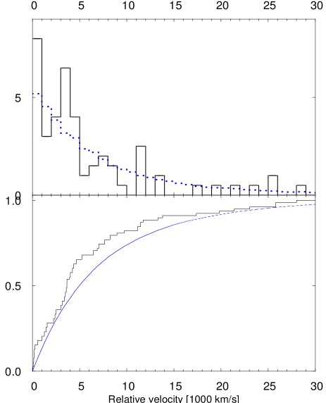
Figure 7: Upper panel: Histogram of the velocity separations between two closest-neighbor C iv absorption systems in our sample of QSO pairs. The distribution expected from a randomly distributed population of C iv systems is shown as the dashed curve. Lower panel: the cumulative distributions of the observed sample of C iv systems (thick curve) is compared to the cumulative distribution of a randomly distributed population of C iv systems (dashed curve). There is a 18% chance probability (KS test) that the distributions differ that much if the two sample are drawn from the same population.

\begin{picture}(9.0,10.0)\centerline{\hbox{\psfig{height=298.75394pt,width=241.84842pt}}} \end{picture}

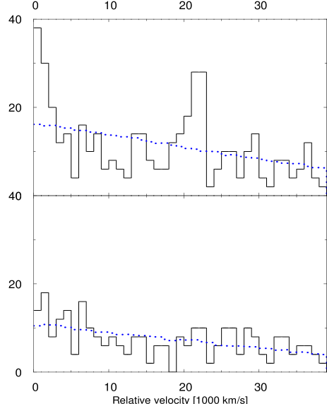
Figure 8: Observed Longitudinal correlation function of C iv systems computed along the 58 lines of sight. The distribution expected from a population of randomly distributed C iv systems is shown as the dashed curve. Upper panel: the whole sample is used. There is an excess on small scales and around 20000 km s^-1. This is due to an excess of correlation along the lines of sight to Q 0103$-$294A,B; Q 0102$-$2931 and Q 0102$-$293 located in the same field (group of quasars). Lower panel: same but without the group.

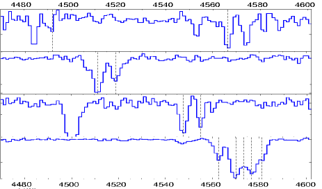
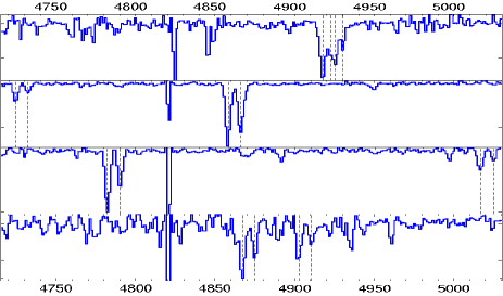
Figure 9: Two sections of the spectra of Q 0103$-$294A&B (separated by 1.3 arcmin) and Q 0102$-$2931 and Q 0102$-$293 (separated by about 6.5 arcmin from Q0103$-$294A,B , see Table 1) in that order from top to bottom. The mean redshifts are 1.93 and 2.14 in the upper and lower panels, respectively. The positions of C iv systems are indicated by dashed vertical lines. There is an overdensity of C iv systems along these lines of sight over the redshift range 1.5 $\leq$ $z$ $\leq$ 2.2 and on a spatial scale larger than 10 arcmin.

6.1 Identifying metal lines

Our sample is also well suited to study the spatial distribution of the gas responsible for the associated metal absorption in QSO spectra. We have manually identified and fitted metal lines in all spectra. The corresponding line lists are compiled in Appendix B (published in the electronic version of the paper) where we report the observed equivalent width, the pixel signal-to-noise ratio at the position of the absorption, the observed wavelength and corresponding redshift for each of the identified metal lines. If applicable the upper limit on the equivalent width of a possible absorption at the same position in the spectrum of the second quasar of the pair is also given.

6.2 The correlation of Civ   systems along adjacent lines of sight

We consider only absorption lines with rest-frame equivalent width $W_{\rm r}$ $>$ 0.1 Å  and redshift intervals common to both lines of sight of a QSO pair. We do not consider systems where N v is detected as these systems are most probably associated with the quasar (see e.g. Petitjean, Rauch & Carswell 1994). We then select the lines that are located at more than 3000  km s^-1  blueward of the QSO Civ  emission line and at more than 1000  km s^-1  redward of the Lyman-$\alpha$ emission line. We end up with a sample of 139 Civ   systems for a redshift path $\delta z=38$, corresponding to a density of 3.7 systems per unit redshift. We apply the Nearest-Neighbor method, as described in Young et al. (2001) and Aracil et al. (2002) to the corresponding list of C iv systems. For each absorption line along one QSO line of sight, we search the adjacent QSO line of sight for the nearest (in velocity) absorption line and construct the histogram of the corresponding velocity differences (see Fig.  7). Our complete sample contains 25 and 39 associations with velocity separations smaller than 5000 and 30000 km s^-1, respectively. To estimate the possible excess of correlation with respect to randomly located absorption lines, we produced 10000 simulated line lists drawn from a population of randomly redshifted lines, taking the same number of lines and the same wavelength ranges as in the observed spectra. The results of applying the same method to the simulated line lists are given as dotted lines in Figure 7.

In the lower panel of Fig. 7 we compare the cumulative distributions of the velocity differences from our observed sample and from a randomly located population of Civ   absorbers. A KS test gives a 18% chance probability that the difference between the two distributions is larger than what is observed if the two samples are drawn from the same population. There is a possible small excess of clustering of Civ   systems on scales smaller than 5000 km s^-1. This scale is larger than the typical correlation length, of about 1000 km s^-1, seen in the longitudinal correlation function of C iv systems (Rauch et al. 1996; Pichon et al. 2003; Boksenberg, Sargent & Rauch 2003; Scannapieco et al. 2006). This is due to an excess of associations in the bin $\Delta v$ $\sim$ 4000 km s^-1. The corresponding C iv associations are located in the peculiar field containing the quartet Q 0103$-$294A&B, Q 0102$-$2931 and Q 0102$-$293 (all four quasars are separated by less than 10 arcmin). In fact, 9 out of the 25 associations with $\Delta v$ $<$ 5000 km s^-1 (see next Section) are found in front of these quasars. If we remove this quartet from the sample, the KS probability is increased to 25%. To ascertain the overdensity in this field, we show in Fig. 8 the longitudinal correlation function for the whole sample (upper panel) and for the sample without the group (lower panel). There is indeed a strong excess in the correlation function of the whole sample for $\Delta v$ $<$ 3000 km s^-1 and around 20000 km s^-1 which disappears when the group is removed from the sample.

The pairs in the current sample have a mean separation larger than 2 arcmin (see Table 1). The correlation at smaller separations can be expected to be larger. Indeed, comparing the results of $N$-body simulations to high spectral resolution observations, Scannapieco et al. (2006) have shown that, at $z\sim 3$, the longitudinal C iv correlation function is consistent with a model where C iv is confined within bubbles of typical radius $\sim$2 Mpc comoving surrounding halos of mass $\sim$ 10¹² M_⊙. At this redshift, this corresponds to a separation of about $\sim$ 2 arcmin. Unfortunately, the small size of our sample prevents any attempt to consider only small separations. Our result is, however, consistent with their findings.

6.3 Peculiarities

It is interesting to note that there is an overdensity of C iv pairs in front of the quartet Q 0103$-$294A&B, Q 0102$-$2931 and Q 0102$-$293. The density of C iv systems along the four lines of sight (6.4 per unit redshift) and the number of coincidences within 4000 km s^-1 is about twice larger than the mean density of coincidences in the overall sample. In Fig. 9 we plot two portions of the spectra of Q0103$-$294A,B (separated by 1.3 arcmin) and Q 0102$-$2931 and Q 0102$-$293 (separated by about 6.5 arcmin from Q0103$-$294A,B , see Table 1). The wavelength ranges of the two portions are centered on $z$ = 1.92 and 2.14, respectively. Note, however, that the overdensity of C iv systems along these lines of sight extends over the much larger redshift range 1.5 $\leq$ $z$ $\leq$ 2.2 and over a spatial scale larger than 10 arcmin (see Appendix B). There are two more peculiarities occurring along these lines of sight. There are no C iv systems between $z$ = 1.955 and 2.051 and there is a quasi-spherical structure of reduced H i absorption with radius $\sim$12.5$h^{-1}$ Mpc at $z$ $\sim$ 1.992 in front of the quartet (Rollinde et al. 2003). Note also that the correlation between the Lyman-$\alpha$ forests of Q 0102$-$2931 and Q 0103$-$294B, two quasars of the group with $\sim$6 arcmin separation, is measured to be quite high ($\xi$ = 0.11, see Table 1 and Fig. 3).

A similar overdensity of C iv systems has been observed in the field of Tol 1037$-$2704 (e.g. Jakobsen et al. 1986; Dinshaw & Impey 1996; Lespine & Petitjean 1997). The overdensity of C iv systems in this field extends over the redshift range $\sim$1.5$-$2.2 and a transverse scale $>$ 15 arcmin and has been interpreted as being due to the presence of a supercluster. The dimensions of this supercluster would be at least 80 and 30$h^{-1}$ Mpc along and perpendicular to the line of sight, respectively. To our knowledge no deep imaging of this field exists. Another overdensity of C iv systems has been reported in front of PKS 0237$-$233 (Sargent, Boksenberg & Steidel 1988; Foltz et al. 1993). The overdensity reported in this work in the field around Q 0103$-$294A,B may give new clues to solve the puzzle of the origin of these overdensities extending over very large scales as the four quasars constituting the quartet are very close to each other. Deep infra-red imaging should be performed in the field to search for any concentration of objects in the corresponding redshift range. High spectral resolution observations of the quasars would allow a more detailed investigation of the nature of these C iv systems.

The pair J 000852.7-290044/J000857.7-290126 is also peculiar as the two lines of sight show 9 and 4 C iv systems respectively, corresponding to 3.5 and 1.5 times the mean density of systems. J 000852.7-290044 shows a BAL systems and it would be interesting to question the intervening origin of some of the narrow systems (Srianand & Petitjean 2001).

7 Conclusions

We have obtained VLT-FORS observations of a large sample of 32 pairs of QSO with separations in the range 0.6 $<$ $\theta$ $<$ 10 arcmin building on the smaller sample of Rollinde et al. (2003) of 11 pairs. We present measurements of the transverse and longitudinal correlation functions from this sample. We further use a large box-size DM only simulation and a somewhat smaller full hydro-dynamical simulation to investigate the effect of spectral resolution, thermal broadening and peculiar motions on the correlation function and to determine realistic error estimates. The longitudinal correlation function from the FORS sample is in good agreement with that obtained from UVES high-resolution data if the effect of the different spectral resolutions is taken into account.

The transverse correlation is detected at the 3 $\sigma$ level up to separations of about $\sim$3$-$5 arcmin. The sample is sufficiently large to obtain a binned estimate of the average correlation function which has about a factor 1.5-2 smaller errors than the smaller sub-sample described in Rollinde et al. (2003). The shape and correlation length of the transverse correlation function of the absorbing gas is in good agreement with expectations for absorption by density fluctuations in the warm photo-ionized Intergalactic Medium as described in CDM-like structure formation models. Our measurement of the transverse correlation function is thus an important further independent confirmation that the Lyman-$\alpha$ forest is indeed caused by the filamentary and sheet-like structures of the cosmic web predicted by these models.

We then use the numerical simulations and predictions of linear theory to assess prospects of using the transverse correlation function for a variant of the Alcock & Paczyński test to determine cosmological parameters. In agreement with predictions of previous theoretical studies we find that our sample is still too small for this purpose. The improved errors of our larger sample compared to the sub-sample of Rollinde et al. (2003) suggest however that meaningful constraints on $\Omega_{\Lambda}$ can be obtained. For this, a larger sample and a careful analysis of the systematic uncertainties with a large suite of full hydrodynamical simulations are necessary. Mc Donald (2003) estimated that this requires a sample of 13($\theta$/1’)² pairs on scales up to 10 arcmin.

We have also used our sample to investigate the transverse and longitudinal correlation functions of C iv absorption systems on the scales probed by our pairs, but did not detect any signal. This is not surprizing as most of the separations are larger than 2 comoving Mpc. This is larger than is expected for the size of metal-enriched bubbles surrounding massive haloes (e.g. Scannapieco et al. 2006). We have, however, detected a prominent overdensity of C iv systems in front of the quartet Q 0103$-$294A&B, Q 0102$-$2931 and Q 0102$-$293 which extends over the redshift range 1.5 $\leq$ $z$ $\leq$ 2.2 and over a spatial scale larger than 10 arcmin. This suggests the presence of a high-redshift cluster in this field and makes it a prime target for deep infra-red imaging.

QSO	$w_{\rm obs}$	$\lambda_{\rm{obs}}$	$z_{\rm abs}$
	(Å)	(Å)
J 135003.0$-$011703	29.6	4055.77	2.336
J 144245.6$-$024251	21.4	3911.52	2.218
J 000852.7$-$290044	22.2	3955.77	2.254
J 000857.7$-$290126	20.0:	4243.08	2.490
Q 2139$-$4504B	55.3	5071.54	3.172

Table 3: Damped Lyman-$\alpha$ system candidates detected in the survey

Appendix A Comments on individual lines of sight

In this Section, we comment on peculiarities of individual observed lines of sight. The quasar emission redshifts (given in Table 1) are determined by fitting a Gaussian profile to the C iv emission line when present in the spectrum or to the Lyman-$\alpha$ emission line otherwise. Damped Lyman-$\alpha$ systems are listed in Table 2 and identified metal lines are given in Tables gathered in the Appendix.

A.1 J 000852.7-290044$-$J 000857.7-290126

QSO J 000852.7-290044 has a BAL system close to the emission redshift with two strong components seen in N v, O vi and C iv. In addition there is a damped Lyman-$\alpha$ system at $z_{\rm abs}$ = 2.254 ($W_{\rm obs}$ = 22.2 Å) with strong associated metallic absorption. There is no corresponding absorption toward J 000857.7-290126 but another damped Lyman-$\alpha$ system is detected at $z_{\rm abs}$ = 2.490 ($W_{\rm obs}$ = 20.0 Å) with O vi and O i associated absorption. Civ   absorption is detected at $z_{\rm abs}$ = 2.218 toward J 000852.7-290044 and at $z_{\rm abs}$ = 2.215 toward J 000857.7-290126 (i.e. with a velocity difference of only 294  km s^-1).

A.2 Q 0103-294A$-$Q 0103-294B

These quasars belong to a group of QSOs described in Rollinde et al. (2003). There is an over-density of Civ systems between $z_{\rm abs}$ = 1.536 and 2.18 observed in front of the group (see also Section 6.2). Alternative names for Q 0103-294A and B are, respectively, J010534.7-290917 and J010538.3-291106.

A.3 Q 0236-2411$-$Q 0236-2413

There are strong but narrow associated absorption features toward Q 0236-2413 close to the Civ , Si iv and N v emission lines.

A.4 J 023836.9-282310$-$J 023849.0-282101

We detect strong metallic absorptions toward QSO J 023836.9-282310 and in particular a strong O vi doublet at $z_{\rm abs}$ = 2.56. The signal to noise ratio of the J 023849.0-282101 spectrum is good but very few metal absorptions are detected except for a strong Mg ii system at $z_{\rm abs}$ = 0.871. In the same spectrum a Civ system may be present at $z_{\rm abs}$ = 2.083 but the $\lambda$1550 transition is under our 3$\sigma$ detection limit.

A.5 UM 680$-$UM 681

This pair has been observed with UVES (see D’Odorico et al. 2002). As discussed by these authors, there is a sub-DLA system (log $N$(H i) = 18.6) toward UM 681 at $z_{\rm abs}$ = 1.788. Noticeably as well, there are two coincident Lyman Limit Systems at $z_{\rm abs}$ = 2.03 and two coincident associated systems at $z_{\rm abs}$ = 2.125.

A.6 J 031036.4-305108$-$J 031041.0-305027

Very few metal absorptions are seen toward J 031036.4-305108 apart from a Civ system at $z_{\rm abs}$ = 1.8. On the contrary, the line of sight toward J 031041.0-305027 shows two metallic systems, one at $z_{\rm abs}$ $\sim$ 2.39 and the other clearly associated with the QSO at $z_{\rm abs}$ $\sim$ 2.542. The two lines of the Si iv doublet for the latter system are under our 3$\sigma$ detection limit but weak features can be seen at the expected positions and N v absorption lines are clearly detected (see Appendix).

A.7 FOCAP QSF:01$-$FOCAP QSF:04

There is a possible Civ doublet at $z_{\rm abs}$ = 2.27 toward FOCAP QSF:01 but the corresponding C iv$\lambda$1550 transition is weaker than our detection limit. Other names for FOCAP QSF:01 and FOCAP QSF:04 are, respectively, J034105.1-445619 and J034126.2-445842.

A.8 J 095800.2-002858$-$J 095810.9-002733

Strong C iv absorption is seen toward J 095810.9-002733 at $z_{\rm abs}$ $\sim$ 1.807 with other metal absorption lines from Al ii, Al iii and C ii; the Lyman-$\alpha$ absorption corresponding to this system is out of the observed wavelength range. Possible N v$\lambda\lambda$1238,1242 absorptions are seen at 4164.5 and 4151.5 Å  but the corresponding features are below the 3$\sigma$ detection limit. A Si iv system may be present at $z_{\rm abs}$ = 2.122 toward J 095800.2-002858.

A.9 J 102827.1-013641$-$J 102832.6-013448

The determination of the emission redshift for J 102827.1-013641 is complicated by the presence of a number of absorptions at a redshift close to the emission redshift: there is a strong Lyman-$\alpha$ system with associated metallic absorption at $z_{\rm abs}$ = 2.399. The determination of $z$ by a Gaussian fit of the Civ emission line gives $z_{\rm em}$ = 2.392. The Fe ii system at $z_{\rm abs}$ = 1.316 has no Mg ii counterpart detected.

A.10 Q 1206-1056$-$Q 1207-1057

Q 1207-1057 shows broad and shallow absorptions at 4885-4955 Å  for Civ , 4385-4500 Å  for S iv and 3900-3974 Å  for N v. The Lyman-$\alpha$ line associated with the BAL system is not clearly detected. There is probably a Mg ii and Fe ii system at $z_{\rm abs}$ $\sim$ 0.772 but most of the corresponding absorptions are under the 3$\sigma$ detection limit.

A.11 J 120725.9-024519$-$J 120734.5-024725

Strong absorptions from Mg ii$\lambda\lambda$2796,2803, Fe ii$\lambda\lambda$2374,2382, Fe ii$\lambda\lambda$2596,2600 and Mgi$\lambda$2852 are detected at $z_{\rm abs}$ = 0.777 toward J 120725.9-024519.

A.12 J 123510.5-010746$-$J 123511.0-010830

The redshift difference between these two quasars is one of the largest in our sample: $z_{\rm em}$ = 2.785 and 2.235 for J 123510.5-010746 and J 123511.0-010830 respectively. There is a $z_{\rm abs}\sim 2.26$ associated Civ system in the spectrum of J 123510.5-010746 at a redshift close to the emission redshift of the QSO.

A.13 J 125556.9+001848$-$J 125606.3+001728

The spectrum of J 125556.9+001848 presents a shallow $z_{\rm abs}\sim 2.08$ Civ absorption feature close to the emission redshift and a strong absorption in the range 3810-3845 Å  that could be identified as the corresponding N v absorption. J 125606.3+001728 shows several strong Civ absorptions that have no counterpart along the adjacent line of sight toward J 125556.9+001848.

A.14 J 135001.7-011703$-$J 135003.0-011819

A damped Lyman-$\alpha$ system is detected toward J 135003.0-011819 at $z_{\rm abs}$ = 2.33 ($W_{\rm obs}$ = 29.6 Å) with associated strong metallic absorption.

A.15 J 141124.6-022943$-$J 141117.3-023222

There is a noticeable decrease of the number of H i absorption lines in the Lyman-$\alpha$ forest of J 141124.6-022943 at the emission redshift of J 141117.3-023222 possibly corresponding to a strong transverse proximity effect.

A.16 J144245.6-024251$-$J144245.7-023906

Toward J 144245.6-024251, there is a damped Lyman-$\alpha$ system at $z_{\rm abs}$ = 2.218 ($W_{\rm obs}$ = 21.4 Å) as well as Zn ii, Cr ii and Fe ii absorptions at $z_{\rm abs}$ = 1.178.

A.17 Q 2129-4653A$-$Q 2129-4653B

There is a strong feature in the two spectra over the wavelength range 4044-4058 Å. In Q2129-4653B we successfully identified this feature as two blended Civ systems with a separation of about 530  km s^-1. Along the other line of sight the lines are heavily blended but could be modelled as C iv absorptions at the same redshift.

A.18 Q 2139-4504B$-$Q 2139-4504A

This is the pair with the smallest separation (0.6 arcmin) and the highest redshift in our sample. The two spectra show a Lyman limit system at a redshift close to the emission redshift of the quasar. There is a strong damped Lyman-$\alpha$ system at $z_{\rm abs}$ = 3.172 ($W_{\rm obs}$ = 55.35 Å) toward Q 2139-4504B with associated C ii and Si ii absorptions. There are no corresponding metal absorptions toward Q 2139-4504A down to $w_{\rm r}$ $<$ 0.3 Å. It is interesting to note that there is a lack of absorption in the Lyman-$\alpha$  forest of Q 2139-4504B at the redshift of Q 2139-4504A suggesting the presence of a strong transverse proximity effect.

A.19 J 214501.6-303121$-$J 214507.0-303046

Associated systems are detected toward both quasars, at $-$1250 and $-$380 km s^-1 relative to the QSO emission redshift toward, respectively, J 214501.6-303121 and J 214507.0-303046.

A.20 J 223850.1-295612$-$J 223850.9-295301

J 223850.9-295301 exhibits broad but shallow absorption lines of Civ and Lyman-$\alpha$.

A.21 J 232800.7-271655$-$J 232804.4-271713

The spectra have a poor signal-to-noise ratio. We identify a possible Mg ii system toward J 232800.7-271655 at $z_{\rm abs}$ = 0.368 (Mg ii$\lambda$2803 and Mg ii$\lambda$2796) but no other species are seen in the spectrum. A strong Civ system may be present in the Lyman-$\alpha$ forest of J 232804.4-271713 at $z_{\rm abs}$ = 1.545.

A.22 Q0102-293   $z_{\rm em}$ = 2.441 and Q0102-2931   $z_{\rm em}$ = 2.212

Alternative names for Q 0102-293 and Q 0102-2931 are, respectively, J010502.8-290618 and J010518.0-291510.

Appendix B Line Lists

Table 4: Line list for J 000852.7-290044 and J 000857.7-290126

	J 000852.7-290044						J 000857.7-290126
	$w_{\rm{obs}}$	S/N	$\lambda_{\rm{obs}}$	Ident	z	$w_{\rm{obs}}$	S/N	$\lambda_{\rm{obs}}$	Ident	z
1	11.21	16	3752.73	OVI_1031	2.6366	$<$0.37
2	7.25	18	3758.33	OVI_1031	2.6420	$<$0.39
3	6.06	21	3773.53	OVI_1037	2.6367	$<$0.51
4	9.25	32	3777.46	OVI_1037	2.6405	$<$0.62
5	1.38	56	3872.01	SiII_1190	2.2527	$<$1.74
6	1.36	57	3882.08	SiII_1193	2.2533	$<$2.45
7	1.27	56	3924.48	SiIII_1206	2.2528	$<$1.29
8	2.14	59	4099.80	SiII_1260	2.2527	$<$1.58
9	$<$0.40					1.00	36	4153.73	SiII_1190	2.4893
10	$<$4.47					4.65	25	4163.35	SiII_1193	2.4890
									HI_1215	2.4247
11	$<$1.34					3.12	30	4210.52	SiIII_1206	2.4899
12	3.06	73	4341.84	CII_1334	2.2535	$<$1.74
13	$<$0.61					0.74	75	4398.81	SiII_1260	2.4900
14						0.33	65	4422.34	…	…
15	$<$0.49					1.36	54	4481.19	SiIV_1393	2.2152
16	6.99	51	4503.10	NV_1238	2.6350	$<$0.24
17	$<$6.61					0.67	47	4509.93	SiIV_1402	2.2150
18	11.67	32	4512.06	NV_1238	2.6422	$<$0.67
19	11.67	32	4512.06	NV_1242	2.6306	$<$0.67
20	9.14	68	4524.40	NV_1242	2.6405	$<$0.26
21	$<$0.12					1.29	39	4549.72	CIV_1548	1.9387
22	$<$0.12					1.26	36	4556.30	CIV_1550	1.9381
23	$<$0.39					0.76	40	4560.91	CIV_1548	1.9459
24	0.69	95	4562.73	…	…
25	$<$0.13					0.25	44	4567.92	CIV_1550	1.9456
26	0.13	87	4609.78	…	…
27	0.31	84	4617.76	…	…
28	$<$0.15					0.89	38	4657.39	CII_1334	2.4899
29	1.95	74	4687.35	CIV_1548	2.0276	$<$0.30
30	1.22	74	4694.78	CIV_1550	2.0274	$<$0.29
31	0.31	79	4706.51	CIV_1548	2.0400	$<$0.29
32	0.12	80	4713.86	CIV_1550	2.0397	$<$0.28
33	1.86	74	4724.13	CII_1334:	2.5399	$<$0.29
34	$<$0.15					1.92	40	4864.55	SiIV_1393	2.4902
35	$<$0.16					1.20	39	4896.14	SiIV_1402	2.4903
36	2.23	74	4934.04	SiIV_1393	2.5401	$<$0.29
37	1.70	73	4965.90	SiIV_1402	2.5401	$<$0.29
38	1.76	74	4965.90	SiII_1526	2.2527	$<$0.28
39	$<$0.15					3.93	34	4977.86	CIV_1548	2.2153
40	0.10	80	4982.21	CIV_1548:	2.2181	$<$4.16
41	$<$0.16					3.75	36	4985.51	CIV_1550	2.2148
42	0.09	80	4991.80	CIV_1550:	2.2189	$<$1.40
43	0.99	77	5035.38	CIV_1548	2.2524	$<$0.26
44	0.58	79	5043.81	CIV_1550	2.2524	$<$0.26
45	0.50	80	5054.50	CIV_1548	2.2648	$<$0.26
46	0.57	79	5064.34	CIV_1550	2.2657	$<$0.26
48	0.58	81	5074.19	SiIV_1393	2.6407	$<$0.71
49						0.69	46	5077.63	…	…
50						0.42	45	5090.90	…	…
51	0.12	84	5099.90	SiIV_1402	2.6356	$<$0.27
52	0.32	83	5110.95	SiIV_1402	2.6435	$<$0.28
54	$<$0.15					1.18	39	5189.68	MgII_2796	0.8559
55	$<$0.15					0.65	39	5202.92	MgII_2803	0.8558
56	0.25	79	5232.63	FeII_1608	2.2532	$<$0.30
57	0.17	76	5348.77	…	…
58	$<$0.63					2.81	35	5403.66	CIV_1548	2.4903
59	0.63	74	5404.58	…	…
60	$<$0.16					2.22	36	5412.86	CIV_1550	2.4904
61	0.77	76	5434.70	AlII_1670	2.2528	$<$0.29
62	3.48	67	5480.92	CIV_1548	2.5402	$<$0.28
63	2.28	72	5489.94	CIV_1550	2.5401	$<$0.27
64	2.04	75	5558.23	CIV_1548	2.5901	$<$0.23
65	1.74	76	5566.59	CIV_1550	2.5895	$<$0.22
66	0.32	85	5590.47	…	…
67	0.73	85	5603.35	…	…
68	7.45	52	5626.55	CIV_1548	2.6342	$<$0.25
69	11.85	25	5638.61	CIV_1548	2.6420	$<$0.27
70	14.90	27	5639.24	CIV_1550	2.6364	$<$0.27
71	6.46	67	5647.15	CIV_1550	2.6415	$<$0.29
72	0.16	96	5667.39	…	…

Table 5: Line list for J 005852.4-272933 and J 005859.1-273038

	J 005852.4-272933						J 005859.1-273038
	$w_{\rm{obs}}$	S/N	$\lambda_{\rm{obs}}$	Ident	z	$w_{\rm{obs}}$	S/N	$\lambda_{\rm{obs}}$	Ident	z
1	$<$3.25					2.44	25	4161.45	SiII_1190	2.4958
2	$<$2.12					2.63	23	4171.79	SiII_1193	2.4960
3	$<$0.40					2.73	25	4217.50	SiIII_1206	2.4956
4	2.14	29	4277.63	CII_1334	2.2053	$<$0.97
				HI_1215	2.519
5	$<$0.30					1.68	43	4406.39	SiII_1260	2.4960
6	0.43	36	4457.53	…	…
7	0.41	34	4468.29	SiIV_1393	2.2059	$<$0.32
8	0.22	34	4496.46	SiIV_1402	2.2054	$<$0.34
9	0.62	33	4508.74	…	…
10	$<$0.41					0.71	30	4560.23	SiII_1304	2.4961
11						0.41	33	4642.71	…	…
13	$<$0.38					1.86	31	4665.65	CII_1334	2.4961
14	0.67	31	4773.01	CIV_1548	2.0829	$<$0.37
15	0.43	32	4778.46	CIV_1550	2.0813	$<$0.38
16	$<$0.40					2.33	27	4872.33	SiIV_1393	2.4958
17	$<$0.40					1.61	29	4903.67	SiIV_1402	2.4957
18	0.67	32	4963.17	CIV_1548	2.2058	$<$0.33
19	0.34	34	4972.17	CIV_1550	2.2062	$<$0.32
20						0.49	39	5006.94	…	…
21	0.36	32	5091.25	…	…
22	$<$0.42					0.90	29	5337.35	SiII_1526	2.4960
23	0.25	29	5338.66	…	…
24	$<$0.39					4.02	25	5411.35	CIV_1548	2.4952
25	$<$0.39					2.97	28	5420.39	CIV_1550	2.4953
26	0.78	29	5652.77	…	…
27	0.96	27	5731.73	…	…

Table 6: Line list for Q0102-2931 and Q0102-293

	Q0102-2931						Q0102-293
	$w_{\rm{obs}}$	S/N	$\lambda_{\rm{obs}}$	Ident	z	$w_{\rm{obs}}$	S/N	$\lambda_{\rm{obs}}$	Ident	z
1	0.22	41	3943.28	CII_1334:	1.9548	$<$0.45
2	0.43	27	4114.44	SiIV_1393	1.9520	$<$2.49
3	0.32	28	4117.41	SiIV_1393	1.9542	$<$0.91
4	0.37	27	4140.48	SiIV_1402	1.9516	$<$0.27
5	0.30	28	4144.54	SiIV_1402	1.9545	$<$0.64
6	$<$0.43					0.74	48	4228.74	CIV_1548	1.7314
7	$<$0.44					0.55	49	4235.21	CIV_1550	1.7310
8	$<$0.43					0.88	44	4305.36	SiIV_1393	2.0890
9	$<$0.45					1.09	40	4332.85	SiIV_1402	2.0888
10						1.62	35	4500.45	…	…
11	$<$0.42					0.44	37	4547.39	CIV_1548	1.9372
12	0.43	30	4547.44	FeII_2382	0.9085	$<$0.44
13	$<$0.40					0.26	37	4554.88	CIV_1550	1.9372
14	1.64	27	4563.04	CIV_1548:	1.9473	$<$0.33
15	3.73	18	4570.51	CIV_1550	1.9472	$<$0.33
				CIV_1548	1.952
16	1.46	18	4573.56	CIV_1548:	1.9541	$<$0.32
17	3.77	18	4576.34	CIV_1550:	1.9510	$<$0.32
18	1.25	24	4581.03	CIV_1550:	1.9540	$<$0.32
19	$<$0.42					1.39	38	4782.31	CIV_1548	2.0889
20	$<$0.43					0.86	40	4790.25	CIV_1550	2.0889
23	0.48	29	4866.89	CIV_1548	2.1436	$<$0.30
24	0.30	30	4874.66	CIV_1550	2.1434	$<$0.30
25	0.35	33	4902.52	CIV_1548	2.1666	$<$0.31
26	0.24	35	4910.43	CIV_1550	2.1664	$<$0.31
27	0.20	39	4935.25	FeII_2586	0.9080	$<$0.32
28	0.11	46	4960.91	FeII_2600	0.9079	$<$0.32
29	$<$0.28					0.48	38	5015.98	CIV_1548	2.2399
30	$<$0.30					0.18	38	5024.29	CIV_1550	2.2398
31	$<$0.34					2.11	34	5071.72	FeII_2344	1.1635
32	$<$0.37					1.48	36	5137.20	FeII_2374	1.1635
33	$<$0.38					2.46	33	5155.22	FeII_2382	1.1635
34	0.58	30	5335.73	MgII_2796	0.9081	$<$0.25
35	0.52	31	5349.39	MgII_2803	0.9081	$<$0.25
38	$<$0.46					2.06	33	5596.51	FeII_2586	1.1636
39	$<$0.47					2.46	33	5625.82	FeII_2600	1.1636

Table 7: Line list for Q0103-294A and Q0103-294B

	Q0103-294A						Q0103-294B
	$w_{\rm{obs}}$	S/N	$\lambda_{\rm{obs}}$	Ident	z	$w_{\rm{obs}}$	S/N	$\lambda_{\rm{obs}}$	Ident	z
1	0.13	63	3904.00	…	…
3	$<$0.20					0.37	49	3925.59	CIV_1548	1.5356
4	$<$0.20					0.26	48	3932.93	CIV_1550	1.5361
5	$<$0.20					0.44	47	3941.42	CIV_1548	1.5458
6	$<$0.20					0.22	49	3947.88	CIV_1550	1.5457
7	$<$0.20					1.76	43	3956.64	CIV_1548:	1.5556
8	$<$0.20					1.25	46	3963.38	CIV_1550:	1.5557
9	2.84	50	4001.65	…	…
10	$<$0.25					0.15	42	4061.08	SiIV_1393	1.9138
11	$<$0.26					0.13	41	4087.95	SiIV_1402	1.9142
12						0.53	42	4187.52	…	…
13	1.28	44	4238.75	CII_1334	2.1762	$<$0.29
14	1.93	42	4270.88	CIV_1548	1.7586	$<$0.28
15	1.23	44	4277.66	CIV_1550	1.7584	$<$0.28
16	$<$0.25					0.98	42	4373.40	SiIV_1393	2.1378
17	$<$0.24					0.56	43	4401.87	SiIV_1402	2.1380
18	0.83	49	4426.89	SiIV_1393	2.1762	$<$0.27
19	0.46	53	4455.40	SiIV_1402	2.1761	$<$0.26
20	0.16	54	4484.33	…	…
21	0.23	55	4484.34	CIV_1548:	1.8965	$<$0.26
22	0.08	55	4500.99	CIV_1550:	1.9024	$<$0.25
23	$<$0.23					0.90	45	4511.06	CIV_1548	1.9137
24	$<$0.23					0.51	45	4518.63	CIV_1550	1.9138
25	0.28	50	4566.26	CIV_1548	1.9494	$<$0.27
26	0.27	50	4574.08	CIV_1550	1.9495	$<$0.28
29	$<$0.25					0.69	44	4724.32	CIV_1548	2.0515
30	$<$0.26					0.37	45	4732.09	CIV_1550	2.0514
31	0.17	46	4759.04	…	…
32	0.45	48	4769.66	…	…
35	$<$0.22					2.70	41	4857.95	CIV_1548	2.1378
36	$<$0.21					2.14	44	4865.95	CIV_1550	2.1377
37	1.40	61	4918.35	CIV_1548	2.1768	$<$0.22
38	0.42	61	4921.98	CIV_1548:	2.1792	$<$0.22
39	0.68	61	4924.78	CIV_1550	2.1757	$<$0.21
40	0.37	65	4929.78	CIV_1550:	2.1789	$<$0.21

Table 8: Line list for J 013734.2-303802 and J 013734.2-304050

	J 013734.2-303802						J 013734.2-304050
	$w_{\rm{obs}}$	S/N	$\lambda_{\rm{obs}}$	Ident	z	$w_{\rm{obs}}$	S/N	$\lambda_{\rm{obs}}$	Ident	z
1	$<$1.00					0.33	58	4128.70	CII_1334	2.0937
2						0.33	44	4216.09	…	…
5	0.46	40	4291.65	…	…
6	0.47	41	4321.63	NV_1238	2.4885	$<$0.31
7	0.21	40	4335.65	NV_1242	2.4886	$<$0.31
9	0.32	37	4353.71	…	…
10	$<$0.40					0.27	39	4500.24	SiIV_1393	2.2289
11	$<$0.40					0.35	40	4529.05	SiIV_1402	2.2286
12	$<$0.41					0.40	44	4636.20	CIV_1548	1.9946
13	$<$0.40					0.30	45	4643.51	CIV_1550	1.9943
14	$<$0.40					0.62	39	4790.69	CIV_1548	2.0944
15	$<$0.39					0.41	40	4798.57	CIV_1550	2.0943
18	$<$0.36					0.65	39	4849.10	CIV_1548	2.1321
19	$<$0.36					0.41	39	4856.68	CIV_1550	2.1318
20	0.96	33	4861.62	SiIV_1393	2.4881	$<$0.31
21	0.22	34	4873.05	…	…
22	0.54	33	4892.82	SiIV_1402	2.4880	$<$0.31
23	$<$0.40					1.16	40	4999.07	CIV_1548	2.2289
24	$<$0.40					0.89	41	5007.56	CIV_1550	2.2291
25	0.32	32	5239.63	…	…
26	2.34	50	5400.30	CIV_1548	2.4881	$<$0.29
27	1.86	48	5409.27	CIV_1550	2.4881	$<$0.29

Table 9: Line list for Q0236-2411 and Q0236-2413

	Q0236-2411						Q0236-2413
	$w_{\rm{obs}}$	S/N	$\lambda_{\rm{obs}}$	Ident	z	$w_{\rm{obs}}$	S/N	$\lambda_{\rm{obs}}$	Ident	z
1	$<$1.37					5.87	25	3947.47	NV_1238	2.1865
2	$<$0.60					6.31	24	3960.15	NV_1242	2.1865
3	$<$1.30					2.69	34	3971.02	NV_1238	2.2055
4	$<$1.44					1.72	38	3984.24	NV_1242	2.2058
6						0.53	35	4007.95	…	…
7	0.82	41	4046.73	NV_1238	2.2666	$<$0.38
8	0.57	40	4059.44	NV_1242	2.2664	$<$0.38
9						1.26	31	4198.12	…	…
10	$<$0.37					0.34	30	4277.66	CII_1334	2.2054
11	0.67	30	4326.23	CIV_1548	1.7944	$<$0.41
12	$<$0.58					0.32	30	4329.38	CIV_1548	1.7964
13	0.52	30	4333.22	CIV_1550	1.7942	$<$0.41
14	$<$0.40					0.24	30	4336.91	CIV_1550	1.7966
15	$<$0.37					1.88	28	4374.74	CIV_1548	1.8257
16	$<$0.36					1.20	28	4382.07	CIV_1550	1.8257
17	$<$0.38					0.97	28	4440.65	SiIV_1393	2.1861
18	$<$0.37					1.81	31	4468.34	SiIV_1393	2.2060
19	$<$0.37					1.81	31	4468.34	SiIV_1402	2.1854
20	$<$0.37					1.41	34	4497.10	SiIV_1402	2.2059
21						0.86	33	4798.68	…	…
23	$<$1.11					0.92	32	4842.83	CIV_1548	2.1280
26	$<$0.35					0.61	33	4850.33	CIV_1550	2.1277
27						0.49	31	4903.63	…	…
28						0.75	32	4914.88	…	…
29	$<$0.33					5.81	24	4933.50	CIV_1548	2.1866
30	$<$0.33					5.28	24	4939.86	CIV_1548	2.1907
31	$<$0.33					5.28	24	4939.86	CIV_1550	2.1854
32	$<$0.33					1.37	36	4949.44	CIV_1550	2.1916
33	$<$0.33					3.65	36	4962.58	CIV_1548	2.2054
34	$<$0.32					3.22	48	4971.20	CIV_1550	2.2056
35	0.64	39	4989.17	CIV_1548	2.2226	$<$0.23
36	0.18	41	4997.53	CIV_1550	2.2226	$<$0.27
37	0.41	47	5057.29	CIV_1548	2.2666	$<$0.33
38	0.40	47	5065.72	CIV_1550	2.2666	$<$0.33
39	0.35	37	5144.38	…	…
40	0.61	36	5229.01	…	…
43	0.76	34	5706.23	…	…

Table 10: Line list for J 023836.9-282310 and J 023849.0-282101

	J 023836.9-282310						J 023849.0-282101
	$w_{\rm{obs}}$	S/N	$\lambda_{\rm{obs}}$	Ident	z	$w_{\rm{obs}}$	S/N	$\lambda_{\rm{obs}}$	Ident	z
1	4.02	22	3671.50	OVI_1031:	2.5579	$<$0.28
2	3.50	28	3691.45	OVI_1037:	2.5576	$<$0.24
4						0.28	84	4385.94	…	…
5	0.53	59	4386.18	FeII_2382	0.8408	$<$0.25
6	4.61	50	4406.52	SiIV_1393	2.1616	$<$0.15
7	4.61	50	4406.52	NV_1238	2.5570	$<$0.15
				SiIV_1393	2.162
8	2.49	52	4421.26	NV_1242	2.5575	$<$0.15
9	0.79	56	4434.20	SiIV_1402	2.1610	$<$0.15
10	$<$0.25					0.42	84	4457.81	FeII_2382	0.8709
11	$<$0.27					0.40	85	4477.99	CIV_1548	1.8924
12	$<$0.27					0.26	86	4485.41	CIV_1550	1.8924
15						0.22	97	4538.02	…	…
16	0.92	38	4547.64	CIV_1548	1.9374	$<$0.13
18	0.47	39	4555.63	CIV_1550	1.9376	$<$0.13
19						0.17	87	4625.12	…	…
20	0.63	39	4740.89	…	…
21	0.43	41	4760.69	FeII_2586	0.8405	$<$0.15
22						0.39	85	4773.10	…	…
23	0.37	41	4784.57	FeII_2600	0.8401	$<$0.14
25	$<$0.31					0.14	87	4839.11	FeII_2586	0.8708
26	$<$0.30					0.50	87	4864.79	FeII_2600	0.8710
27	4.48	32	4894.12	CIV_1548	2.1612	$<$0.38
28	$<$3.02					0.31	89	4896.23	CIV_1548	2.1625
29	1.67	33	4901.45	CIV_1550	2.1606	$<$0.17
30	$<$1.42					0.22	90	4904.00	CIV_1550	2.1623
31	0.26	41	5042.31	…	…
32	0.92	38	5146.51	MgII_2796	0.8404	$<$0.13
33	0.62	40	5159.36	MgII_2803	0.8403	$<$0.14
34	0.68	39	5173.96	…	…
37	$<$0.31					2.42	84	5231.69	MgII_2796	0.8709
38	$<$0.30					1.63	85	5245.00	MgII_2803	0.8709
41	0.17	40	5329.20	…	…
46	2.53	50	5507.65	CIV_1548	2.5574	$<$0.15
47	1.88	53	5515.96	CIV_1550	2.5569	$<$0.15
53	0.62	38	5741.97	…	…

Table 11: Line list for J 031036.4-305108 and J 031041.0-305027

	J 031036.4-305108						J 031041.0-305027
	$w_{\rm{obs}}$	S/N	$\lambda_{\rm{obs}}$	Ident	z	$w_{\rm{obs}}$	S/N	$\lambda_{\rm{obs}}$	Ident	z
1	1.11	17	3736.42	CII_1334	1.7998	$<$0.62
				HI_1215	2.074
2	0.68	52	4334.83	CIV_1548	1.7999	$<$0.20
3	0.78	48	4341.97	CIV_1550	1.7999	$<$0.21
4	0.28	40	4380.07	…	…
5	$<$0.31					0.81	51	4388.24	NV_1238	2.5423
6	0.48	38	4393.47	NV_1238:	2.5465	$<$0.24
7	$<$0.32					0.47	49	4402.48	NV_1242	2.5424
8	0.54	38	4407.88	NV_1242:	2.5467	$<$0.25
9						0.28	48	4412.16	…	…
12	$<$0.43					0.65	33	4649.20	MgII_2796	0.6626
13	$<$0.45					0.62	33	4661.19	MgII_2803	0.6626
14	0.37	26	4677.29	AlII_1670	1.7995	$<$0.37
15	$<$0.47					1.12	32	4725.06	SiIV_1393	2.3902
16	$<$0.46					0.57	33	4754.80	SiIV_1402	2.3896
17	0.77	26	5079.98	…	…
18	0.85	26	5193.08	AlIII_1854	1.7999	$<$0.39
19	0.69	27	5215.09	AlIII_1862	1.7996	$<$0.38
20	$<$0.45					2.89	27	5247.96	CIV_1548	2.3897
21	$<$0.45					2.35	26	5256.67	CIV_1550	2.3897
22	$<$0.31					0.94	46	5484.23	CIV_1548	2.5423
23	$<$0.70					0.95	46	5494.10	CIV_1550	2.5428
24	1.13	42	5499.14	CIV_1548	2.5519	$<$0.51
25	0.32	45	5507.67	CIV_1550	2.5515	$<$0.26

Table 12: Line list for J 031054.7-293436 and J 031103.0-293306

	J 031054.7-293436						J 031103.0-293306
	$w_{\rm{obs}}$	S/N	$\lambda_{\rm{obs}}$	Ident	z	$w_{\rm{obs}}$	S/N	$\lambda_{\rm{obs}}$	Ident	z
1	$<$0.50					0.98	59	3892.20	CIV_1548	1.5140
2	$<$0.73					0.68	58	3898.58	CIV_1550	1.5139
4	0.52	34	4073.00	…	…
5	0.68	35	4081.17	NV_1238	2.2944	$<$0.29
6	0.36	34	4094.45	NV_1242	2.2945	$<$0.29
7	0.53	31	4115.50	…	…
8	2.35	22	4147.96	CIV_1548	1.6792	$<$0.28
9	1.95	24	4154.59	CIV_1550	1.6790	$<$0.28
10						0.51	43	4215.17	…	…
11	$<$0.49					0.36	43	4250.35	SiII_1526	1.7840
12	$<$0.48					0.45	43	4260.84	SiIV_1393	2.0571
13	$<$0.47					0.17	44	4288.34	SiIV_1402	2.0570
14	$<$0.46					1.46	39	4309.49	CIV_1548	1.7835
15	$<$0.45					1.16	40	4316.74	CIV_1550	1.7836
16	0.60	26	4451.52	…	…
17	1.01	27	4571.43	CIV_1548	1.9527	$<$0.28
18	0.67	29	4579.09	CIV_1550	1.9528	$<$0.28
19	$<$0.43					0.40	43	4651.62	AlII_1670	1.7841
20	$<$0.46					1.18	42	4734.55	CIV_1548	2.0581
21	$<$0.46					0.66	43	4741.44	CIV_1550	2.0575
22	1.36	24	4803.28	CIV_1548	2.1025	$<$0.27
23	1.18	24	4811.15	CIV_1550	2.1024	$<$0.27
24	1.34	24	4824.74	CIV_1548	2.1163	$<$0.26
25	0.70	25	4832.44	CIV_1550	2.1161	$<$0.26
27	0.49	30	4989.28	…	…
28	0.31	37	5089.95	…	…
29	2.12	34	5099.89	CIV_1548	2.2941	$<$0.26
30	1.33	36	5109.04	CIV_1550	2.2945	$<$0.26
32						0.34	45	5332.70	…	…

Table 13: Line list for FOCAP QSF:01 and FOCAP QSF:04

	FOCAP QSF:01						FOCAP QSF:04
	$w_{\rm{obs}}$	S/N	$\lambda_{\rm{obs}}$	Ident	z	$w_{\rm{obs}}$	S/N	$\lambda_{\rm{obs}}$	Ident	z
1	1.65	19	3791.80	FeII_2382	0.5913	$<$0.38
2	$<$1.37					0.52	29	3823.11	SiIV_1393	1.7430
3	$<$0.48					0.48	28	3848.52	SiIV_1402	1.7435
4	3.10	34	3930.54	AlII_1670:	1.3525	$<$0.46
7	0.39	45	4044.94	NV_1238	2.2652	$<$0.43
8	$<$0.27					1.43	26	4054.02	CIV_1548	1.6185
9	0.20	46	4058.02	NV_1242	2.2652	$<$0.97
10	$<$0.27					1.09	27	4060.75	CIV_1550	1.6185
11	1.33	33	4116.56	FeII_2586	0.5915	$<$0.42
12	1.91	31	4137.98	FeII_2600	0.5914	$<$0.43
13	0.43	30	4215.48	SiIV_1393	2.0245	$<$0.41
14	0.20	32	4243.73	SiIV_1402	2.0252	$<$0.88
15	$<$0.40					1.28	29	4246.98	CIV_1548	1.7432
16	$<$0.40					0.93	31	4253.98	CIV_1550	1.7431
17	0.27	31	4312.60	MgII_2796:	0.5422	$<$0.38
18	0.44	31	4324.10	MgII_2803:	0.5424	$<$0.39
19	0.48	31	4362.17	AlIII_1854	1.3519	$<$0.40
20	0.25	32	4380.82	AlIII_1862	1.3517	$<$0.41
21	2.63	26	4450.23	MgII_2796	0.5914	$<$0.42
22	2.41	27	4461.48	MgII_2803	0.5914	$<$0.42
23	0.80	33	4540.16	…	…
26	0.34	33	4617.83	…	…
27	$<$0.38					0.31	33	4664.28	MgII_2796	0.6680
28	$<$0.38					0.34	35	4675.60	MgII_2803	0.6678
29	0.26	32	4683.17	CIV_1548	2.0249	$<$0.35
30	0.09	32	4691.49	CIV_1550	2.0252	$<$0.34
31	$<$0.39					0.56	39	4754.20	CIV_1548	2.0708
32	$<$0.39					0.24	39	4761.86	CIV_1550	2.0706
33	0.45	29	4825.01	…	…
34	0.89	29	4844.89	…	…
35	0.34	31	4850.60	…	…
36	0.52	44	5053.84	…	…
37	0.77	38	5110.22	MgII_2796	0.8275	$<$0.39
38	0.37	38	5122.72	MgII_2803	0.8272	$<$0.39
39	0.38	33	5291.97	…	…
40	0.44	33	5317.38	…	…
44	3.05	27	5514.02	FeII_2344	1.3522	$<$0.42
45	2.36	27	5584.65	FeII_2374	1.3520	$<$0.43
46	3.76	25	5604.89	FeII_2382	1.3523	$<$0.44

Table 14: Line list for J 095800.2-002858 and J 095810.9-002733

	J 095800.2-002858						J 095810.9-002733
	$w_{\rm{obs}}$	S/N	$\lambda_{\rm{obs}}$	Ident	z	$w_{\rm{obs}}$	S/N	$\lambda_{\rm{obs}}$	Ident	z
1	$<$1.69					5.47	10	3745.16	CII_1334	1.8063
									HI_1215	2.0807
2	$<$0.69					2.83	16	3937.55	SiIV_1402	1.8070
									HI_1215	2.2390
3	2.22	31	4144.25	CIV_1548	1.6768	$<$3.98
4	2.24	30	4151.67	CIV_1550	1.6771	$<$1.03
5	0.80	33	4166.82	CII_1334	2.1223	$<$0.63
6	1.42	18	4338.31	SiIV_1393	2.1127	$<$0.30
7	$<$1.35					6.88	35	4345.74	CIV_1548	1.8070
8	1.44	19	4351.30	SiIV_1393	2.1220	$<$4.05
9	$<$0.91					4.60	31	4352.28	CIV_1550	1.8065
10	0.84	20	4366.54	SiIV_1402	2.1128	$<$0.23
11	0.58	21	4379.53	SiIV_1402	2.1221	$<$0.24
12	$<$0.55					2.40	32	4460.73	SiIV_1393	2.2005
13	$<$0.52					1.09	33	4490.93	SiIV_1402	2.2015
14	$<$0.52					1.56	33	4491.24	SiIV_1393	2.2224
15	$<$0.52					0.79	32	4528.58	SiIV_1402	2.2283
16	$<$0.44					4.30	27	4687.29	AlII_1670:	1.8054
17	0.24	25	4765.54	…	…
18	2.91	19	4819.77	CIV_1548	2.1131	$<$0.38
19	1.68	17	4827.44	CIV_1550	2.1129	$<$0.39
20	2.83	18	4832.54	CIV_1548	2.1214	$<$0.37
21	1.57	20	4842.14	CIV_1550	2.1224	$<$0.37
22	1.10	22	4855.92	…	…
24	$<$0.51					0.74	31	4869.18	CIV_1548	2.1450
25	$<$0.50					0.32	32	4878.13	CIV_1550	2.1456
27	$<$0.51					1.39	32	4954.16	CIV_1548	2.1999
28	$<$0.50					0.43	35	4963.93	CIV_1550	2.2009
29	$<$0.49					2.62	30	4988.67	CIV_1548	2.2222
30	$<$0.50					1.54	32	4996.40	CIV_1550	2.2219
33	0.44	40	5198.17	…	…
34	$<$0.30					1.52	30	5206.14	AlIII_1854	1.8070
35	0.98	40	5216.86	CIV_1548	2.3696	$<$0.37
36	0.37	43	5224.94	CIV_1550	2.3692	$<$0.44
37	$<$0.38					0.92	32	5229.07	AlIII_1862	1.8071
38						1.09	37	5384.46	…	…

Table 15: Line list for J 102827.1-013641 and J 102832.6-013448

	J 102827.1-013641						J 102832.6-013448
	$w_{\rm{obs}}$	S/N	$\lambda_{\rm{obs}}$	Ident	z	$w_{\rm{obs}}$	S/N	$\lambda_{\rm{obs}}$	Ident	z
1	$<$0.90					1.09	21	3878.17	CII_1334	1.9060
									HI_1215	2.1901
2	2.21	15	4046.38	SiII_1190	2.3991	$<$0.57
3	$<$0.79					0.97	35	4050.95	SiIV_1393	1.9065
4	0.60	17	4055.78	SiII_1193	2.3988	$<$0.33
5	$<$1.19					0.73	37	4076.75	SiIV_1402	1.9062
6	1.25	18	4100.24	SiIII_1206	2.3985	$<$0.33
				HI_1215	2.373
7	1.27	17	4284.16	SiII_1260	2.3990	$<$0.46
8	$<$0.66					1.14	24	4295.69	AlIII_1854:	1.3161
9	$<$0.63					0.61	27	4313.54	AlIII_1862	1.3156
10	1.33	17	4336.08	CIV_1548	1.8007	$<$0.48
11	0.99	17	4342.22	CIV_1550	1.8000	$<$0.48
12						0.54	26	4397.48	…	…
13	0.96	16	4425.98	OI_1302	2.3989	$<$0.62
14						0.62	25	4426.65	…	…
15	0.97	18	4434.09	SiII_1304	2.3994	$<$0.49
16						0.45	25	4435.87	…	…
17	2.61	14	4487.30	…	…
18	$<$0.71					1.92	23	4499.88	CIV_1548	1.9065
19	$<$0.71					1.72	24	4506.98	CIV_1550	1.9063
20	1.50	15	4535.54	CII_1334	2.3986	$<$0.46
21	2.72	17	4551.01	…	…
22	0.90	18	4675.95	CIV_1548	2.0202	$<$0.46
23	0.45	19	4683.39	CIV_1550	2.0200	$<$0.47
24	2.04	18	4736.78	SiIV_1393	2.3986	$<$0.48
25	1.18	21	4767.95	SiIV_1402	2.3989	$<$0.49
26						0.57	25	4876.82	…	…
27						2.25	25	4887.16	…	…
28	3.43	16	4911.02	…	…
29						0.65	29	4994.75	…	…
30	0.92	21	5189.15	SiII_1526	2.3989	$<$0.44
31	2.16	24	5261.44	CIV_1548	2.3984	$<$0.45
32	1.51	26	5270.60	CIV_1550	2.3987	$<$0.44
34	$<$0.62					3.41	24	5428.51	FeII_2344	1.3157
35	1.49	18	5451.81	…	…
36	0.70	18	5475.35	…	…
37	$<$0.58					1.92	25	5498.56	FeII_2374	1.3157
38	$<$0.61					4.20	22	5517.79	FeII_2382	1.3157
39	1.37	19	5630.72	…	…
41	0.95	16	5679.01	AlII_1670	2.3990	$<$0.45
43						0.56	25	5731.92	…	…

Table 16: Line list for J 111200.4-013242 and J 111201.8-013018

	J 111200.4-013242						J 111201.8-013018
	$w_{\rm{obs}}$	S/N	$\lambda_{\rm{obs}}$	Ident	z	$w_{\rm{obs}}$	S/N	$\lambda_{\rm{obs}}$	Ident	z
1	$<$0.81					1.64	43	3933.49	SiIV_1393	1.8222
2	$<$1.72					1.06	50	3959.22	SiIV_1402	1.8224
3	0.24	50	4127.70	…	…
4	0.32	45	4151.18	CIV_1548	1.6813	$<$0.74
5	0.48	46	4157.79	CIV_1550	1.6811	$<$0.21
6	0.27	39	4194.57	CIV_1548	1.7093	$<$0.40
7	0.25	40	4202.22	CIV_1550	1.7097	$<$0.52
9	$<$0.31					1.35	82	4362.97	CIV_1548	1.8181
10	$<$0.31					0.78	81	4370.12	CIV_1550	1.8180
11	$<$0.30					0.68	80	4396.84	NV_1238	2.5492
12	$<$0.29					0.23	82	4404.75	NV_1242	2.5442
13	$<$0.29					0.90	63	4494.26	CIV_1548	1.9029
14	$<$0.29					0.56	62	4501.22	CIV_1550	1.9025
15	0.37	43	4535.94	…	…
16	0.96	50	4616.26	…	…
17	0.54	46	4646.14	…	…
18						0.21	59	4671.42	…	…
19	0.64	41	4676.47	…	…
21						0.32	57	4716.14	…	…
22	0.67	38	4866.52	CIV_1548:	2.1433	$<$0.21
23	0.40	39	4873.27	CIV_1550:	2.1425	$<$0.21
24	0.82	37	4881.60	MgII_2796	0.7457	$<$0.20
25						0.14	60	4890.22	…	…
26	0.43	39	4894.66	MgII_2803	0.7459	$<$0.20
27	$<$0.29					0.19	67	4972.09	SiIV_1393:	2.5674
28	0.57	45	5038.37	CIV_1548	2.2543	$<$0.20
29	0.42	47	5047.34	CIV_1550	2.2547	$<$0.20
30	0.24	56	5105.27	…	…
31	$<$0.29					1.57	53	5205.01	CIV_1548	2.3620
32	$<$0.30					1.14	53	5213.72	CIV_1550	2.3620
33	$<$0.31					0.28	55	5283.52	CIV_1548	2.4127
34	$<$0.30					0.12	55	5292.33	CIV_1550	2.4127
36	$<$0.30					0.61	66	5488.32	CIV_1548	2.5450
37	$<$0.30					0.57	69	5495.51	CIV_1550	2.5437
38	$<$0.30					0.79	68	5523.19	CIV_1548	2.5675
39	$<$0.31					0.44	66	5532.46	CIV_1550	2.5675
43						0.58	53	5731.16	…	…

Table 17: Line list for J 112108.2+003420 and J 112116.1+003112

	J 112108.2+003420						J 112116.1+003112
	$w_{\rm{obs}}$	S/N	$\lambda_{\rm{obs}}$	Ident	z	$w_{\rm{obs}}$	S/N	$\lambda_{\rm{obs}}$	Ident	z
1	0.32	46	3935.02	…	…
2						0.51	31	4019.10	…	…
3	0.40	36	4065.07	…	…
4	0.58	34	4085.84	CII_1334	2.0616	$<$0.42
5						0.65	27	4125.55	…	…
6						0.58	25	4246.95	…	…
7	1.23	34	4267.73	SiIV_1393	2.0620	$<$1.32
8						1.89	26	4279.14	…	…
9	1.14	33	4295.44	SiIV_1402	2.0621	$<$0.44
10						0.31	30	4464.20	…	…
11	0.53	38	4492.89	…	…
12	$<$0.34					1.00	27	4553.79	CIV_1548	1.9413
13	$<$0.34					0.68	27	4561.16	CIV_1550	1.9412
14	0.66	35	4660.61	…	…
15	$<$0.35					0.85	26	4668.46	CIV_1548	2.0154
16	$<$0.35					0.70	27	4675.78	CIV_1550	2.0151
17	$<$0.34					1.46	26	4717.58	CIV_1548	2.0471
18	$<$0.34					1.16	27	4725.59	CIV_1550	2.0472
19	1.54	34	4741.18	CIV_1548	2.0624	$<$0.43
20	1.51	33	4748.41	CIV_1550	2.0619	$<$0.43
21						0.44	28	4793.89	…	…
22	$<$0.27					1.97	46	4976.65	CIV_1548	2.2145
23	$<$0.28					0.97	43	4985.13	CIV_1550	2.2146
25						0.39	30	5374.31	…	…
26	$<$0.34					0.86	28	5407.04	MgII_2796:	0.9336
27	$<$0.34					0.50	28	5419.57	MgII_2803:	0.9331

Table 18: Line list for J 120725.9-024519 and J 120734.5-024725

	J 120725.9-024519						J 120734.5-024725
	$w_{\rm{obs}}$	S/N	$\lambda_{\rm{obs}}$	Ident	z	$w_{\rm{obs}}$	S/N	$\lambda_{\rm{obs}}$	Ident	z
1	$<$1.10					0.26	41	3985.24	CII_1334	1.9862
2						0.76	28	4129.70	…	…
3						0.91	27	4162.23	…	…
4	1.99	31	4235.65	FeII_2382	0.7776	$<$0.42
5	$<$2.40					1.74	26	4323.53	CIV_1548	1.7926
6	$<$0.33					1.67	26	4330.54	CIV_1550	1.7925
7						0.22	32	4528.50	…	…
8	1.56	54	4548.92	NV_1238	2.6720	$<$0.36
9	1.25	53	4563.67	NV_1242	2.6721	$<$0.36
10	0.59	44	4597.41	FeII_2586	0.7774	$<$0.40
11	0.91	38	4622.01	FeII_2600	0.7776	$<$1.25
12	$<$0.97					1.86	27	4623.96	CIV_1548	1.9867
13	$<$0.30					1.19	28	4631.06	CIV_1550	1.9863
14	0.58	36	4685.33	CIV_1548:	2.0263	$<$0.42
15	0.38	36	4693.78	CIV_1550:	2.0267	$<$0.42
17	1.53	34	4970.20	MgII_2796	0.7774	$<$0.33
18	1.08	33	4983.03	MgII_2803	0.7774	$<$0.32
21	1.65	52	5685.12	CIV_1548	2.6721	$<$0.46
22	1.33	53	5694.60	CIV_1550	2.6721	$<$0.45

Table 19: Line list for Q 1206-1056 and Q 1207-1057

	Q 1206-1056						Q 1207-1057
	$w_{\rm{obs}}$	S/N	$\lambda_{\rm{obs}}$	Ident	z	$w_{\rm{obs}}$	S/N	$\lambda_{\rm{obs}}$	Ident	z
1	0.28	58	4064.12	…	…
2	0.42	44	4152.90	SiIV_1393	1.9796	$<$0.74
3	0.24	41	4178.74	SiIV_1402	1.9789	$<$0.76
4	$<$0.34					5.30	50	4236.43	NV_1238	2.4197
5	0.97	34	4244.90	SiIV_1393	2.0456	$<$3.32
6	$<$0.35					3.95	49	4249.23	NV_1242	2.4191
7	0.46	35	4272.25	SiIV_1402	2.0456	$<$0.20
8						0.28	60	4276.06	…	…
9	$<$0.34					1.02	57	4289.60	NV_1238	2.4626
10	$<$0.34					1.25	54	4302.66	NV_1242	2.4621
11						0.30	51	4335.88	…	…
12	0.97	40	4611.88	CIV_1548	1.9789	$<$0.27
13	0.33	42	4619.99	CIV_1550	1.9791	$<$0.26
14						0.34	45	4712.18	…	…
15	1.90	34	4715.08	CIV_1548	2.0455	$<$0.32
16	1.25	34	4723.00	CIV_1550	2.0456	$<$0.26
17						1.28	46	4750.74	…	…
18	0.91	35	4779.70	CIV_1548	2.0873	$<$0.25
19	0.51	35	4787.98	CIV_1550	2.0875	$<$0.25
20						0.36	50	4793.47	…	…
21	$<$0.34					1.19	51	4835.93	SiIV_1393	2.4697
22						0.49	51	4857.82	…	…
23	$<$0.34					0.54	51	4866.50	SiIV_1402	2.4692
24	1.50	36	4954.54	MgII_2796	0.7718	$<$0.26
25	0.92	37	4967.29	MgII_2803	0.7718	$<$0.26
26						0.55	46	5163.93	…	…
30						1.37	49	5227.09	…	…
31	$<$0.30					1.34	49	5247.77	CIV_1548	2.3896
32	$<$0.30					0.77	50	5258.31	CIV_1550	2.3907
33						0.79	50	5275.34	…	…
34	$<$0.31					2.43	44	5297.09	CIV_1548	2.4214
35	$<$0.30					1.64	47	5302.08	CIV_1550	2.4190
36						0.26	50	5313.11	…	…
37	$<$0.31					0.97	50	5360.70	CIV_1548	2.4625
38	$<$0.31					5.16	40	5371.25	CIV_1550	2.4636
									CIV_1548	2.4694
39	$<$0.31					2.25	45	5381.44	CIV_1550	2.4701

Table 20: Line list for J 123510.5-010746 and J 123511.0-010830

	J 123510.5-010746						J 123511.0-010830
	$w_{\rm{obs}}$	S/N	$\lambda_{\rm{obs}}$	Ident	z	$w_{\rm{obs}}$	S/N	$\lambda_{\rm{obs}}$	Ident	z
1	$<$0.48					1.44	15	3627.43	SiIV_1393	1.6026
2	$<$0.42					1.42	18	3650.60	SiIV_1402	1.6024
3	$<$0.24					1.08	50	3946.92	CIV_1548	1.5494
4	$<$1.44					0.78	45	3953.77	CIV_1550	1.5495
5						1.00	42	3974.10	…	…
6	$<$0.24					2.57	35	4029.43	CIV_1548	1.6027
7	$<$0.30					2.34	34	4036.12	CIV_1550	1.6026
8						2.99	32	4193.30	…	…
9						0.37	37	4318.36	…	…
10	$<$1.28					1.34	32	4348.96	AlII_1670	1.6029
11	$<$0.19					2.23	32	4797.41	CIV_1548	2.0987
12	$<$0.20					1.64	34	4805.60	CIV_1550	2.0988
13	$<$0.21					0.94	36	4827.95	AlIII_1854	1.6031
14	$<$0.21					0.63	38	4848.76	AlIII_1862	1.6030
15	0.24	57	4889.18	…	…
16	1.12	53	5015.39	CIV_1548	2.2395	$<$0.23
17	0.60	54	5023.48	CIV_1550	2.2393	$<$0.24
18	0.29	58	5080.15	CIV_1548	2.2813	$<$0.31
19	0.30	57	5088.41	CIV_1550	2.2812	$<$0.32
20	0.29	56	5119.20	…	…
21	0.23	57	5132.99	…	…

Table 21: Line list for J 125556.9+001848 and J 125606.3+001728

	J 125556.9+001848						J 125606.3+001728
	$w_{\rm{obs}}$	S/N	$\lambda_{\rm{obs}}$	Ident	z	$w_{\rm{obs}}$	S/N	$\lambda_{\rm{obs}}$	Ident	z
1						0.52	35	3807.24	…	…
2	0.53	32	3828.92	…	…
3	$<$0.31					1.01	31	3862.21	SiII_1526	1.5298
4	$<$0.40					2.02	27	3916.36	CIV_1548	1.5296
5	$<$0.40					1.78	27	3922.86	CIV_1550	1.5296
6	$<$0.41					1.00	30	4030.35	CII_1334	2.0200
7	$<$0.40					1.24	30	4209.25	SiIV_1393	2.0201
8	$<$0.39					0.97	30	4226.41	AlII_1670	1.5296
9	$<$0.39					1.19	31	4236.63	SiIV_1402	2.0202
10	$<$0.38					0.87	35	4298.79	SiIV_1393	2.0843
11	$<$0.36					0.68	35	4327.13	SiIV_1402	2.0847
12	0.80	34	4346.89	CIV_1548	1.8077	$<$0.36
13	0.36	35	4354.25	CIV_1550	1.8078	$<$0.36
14	$<$0.37					0.83	32	4384.49	CIV_1548	1.8320
15	$<$0.38					0.46	32	4391.03	CIV_1550	1.8315
16	$<$0.40					0.45	32	4581.85	MgII_2796:	0.6385
17	$<$0.39					0.44	33	4593.31	MgII_2803:	0.6384
18	$<$0.38					0.31	33	4610.20	SiII_1526	2.0197
19	$<$0.36					2.86	31	4675.83	CIV_1548	2.0202
20	$<$0.36					2.10	30	4683.55	CIV_1550	2.0201
21	$<$0.36					0.51	35	4691.91	AlIII_1854	1.5297
22	$<$0.36					0.40	37	4711.68	AlIII_1862	1.5294
23	0.64	34	4737.61	CIV_1548	2.0601	$<$0.31
24	0.60	34	4745.94	CIV_1550	2.0604	$<$0.30
25	$<$0.33					2.27	44	4774.57	CIV_1548	2.0839
26	$<$0.44					1.25	46	4782.69	CIV_1550	2.0841
27	0.44	40	4784.35	CIV_1548	2.0903	$<$0.91
28	0.27	44	4792.77	CIV_1550	2.0906	$<$0.26
29	0.24	53	4818.05	…	…
30	$<$0.36					0.50	37	5045.44	AlII_1670	2.0198

Table 22: Line list for J 135001.7-011703 and J 135003.0-011819

	J 135001.7-011703						J 135003.0-011819
	$w_{\rm{obs}}$	S/N	$\lambda_{\rm{obs}}$	Ident	z	$w_{\rm{obs}}$	S/N	$\lambda_{\rm{obs}}$	Ident	z
1	2.28	51	3863.44	MgII_2796	0.3816	$<$0.87
2	1.04	56	3872.57	MgII_2803	0.3813	$<$0.93
3	0.40	43	3908.55	…	…
4	0.47	43	3937.48	NV_1238	2.1784	$<$0.80
5	0.37	45	3950.47	NV_1242	2.1787	$<$2.36
6	$<$0.31					4.13	11	3969.05	SiII_1190	2.3342
7	$<$0.34					5.85	10	3980.30	SiII_1193	2.3356
8	3.05	26	4019.18	CIV_1548	1.5960	$<$2.57
9	$<$3.20					5.60	9	4023.80	SiIII_1206	2.3351
10	1.77	27	4024.81	CIV_1550	1.5953	$<$2.91
11	$<$0.43					4.66	9	4203.55	SiII_1260	2.3350
14	0.67	28	4329.50	…	…
15	$<$0.42					4.15	10	4342.08	OI_1302	2.3345
16	$<$0.42					3.42	18	4350.76	SiII_1304	2.3355
17	0.48	30	4357.76	…	…
18	$<$0.50					8.81	42	4451.15	CII_1334	2.3354
20	0.53	37	4465.46	…	…
24						0.48	21	4623.58	…	…
25	$<$0.40					4.19	17	4648.85	SiIV_1393	2.3355
26	$<$0.40					1.75	18	4679.18	SiIV_1402	2.3357
27	0.83	31	4792.42	CIV_1548	2.0955	$<$0.54
28	0.27	32	4799.76	CIV_1550	2.0951	$<$0.54
29	1.92	30	4809.41	CIV_1548	2.1064	$<$0.58
30	1.56	30	4816.95	CIV_1550	2.1061	$<$0.59
31						0.86	20	4858.18	…	…
32	0.56	40	4864.81	…	…
34						2.22	20	4910.26	…	…
35	0.37	53	4921.56	CIV_1548	2.1789	$<$0.60
36	0.17	56	4929.84	CIV_1550	2.1789	$<$0.57
39	$<$0.35					3.79	18	5091.70	SiII_1526	2.3351
40	$<$0.35					4.74	11	5166.22	CIV_1548	2.3369
41	$<$0.36					2.93	16	5173.72	CIV_1550	2.3362
42	$<$0.38					2.71	17	5364.37	FeII_1608	2.3351
43	$<$0.39					0.98	19	5374.09	FeII_1611	2.3355
44						3.13	19	5454.58	…	…
45	$<$0.38					1.34	17	5569.91	AlII_1670	2.3337
46	$<$0.40					0.65	30	5639.95	CIV_1548	2.6429
47	$<$0.40					0.37	32	5648.92	CIV_1550	2.6426
48	$<$0.40					1.68	39	5671.44	CIV_1548	2.6632
49	$<$0.40					1.36	39	5681.35	CIV_1550	2.6635

Table 23: Line list for J 141124.6-022943 and J 141117.3-023222

	J 141124.6-022943						J 141117.3-023222
	$w_{\rm{obs}}$	S/N	$\lambda_{\rm{obs}}$	Ident	z	$w_{\rm{obs}}$	S/N	$\lambda_{\rm{obs}}$	Ident	z
1	$<$2.11					0.87	65	4104.61	NV_1238	2.3133
2	$<$6.53					1.18	63	4117.01	NV_1242	2.3127
3	$<$6.53					1.17	64	4117.01	SiIV_1393	1.9539
4	$<$0.29					0.52	58	4142.86	SiIV_1402	1.9533
5	$<$1.33					1.25	48	4386.90	SiIV_1393	2.1475
6	$<$0.86					0.87	50	4415.04	SiIV_1402	2.1474
7	$<$0.16					1.62	50	4572.28	CIV_1548	1.9533
8	$<$0.16					0.98	52	4580.08	CIV_1550	1.9534
11	0.27	58	4635.05	CIV_1548	1.9938	$<$0.21
12	$<$0.29					0.37	57	4640.29	CIV_1548	1.9972
13	0.15	58	4644.79	CIV_1550	1.9951	$<$0.22
14	$<$0.22					0.23	58	4647.60	CIV_1550	1.9969
15	1.79	46	4718.27	MgII_2796	0.6873	$<$0.23
16	1.40	48	4730.79	MgII_2803	0.6874	$<$0.24
17	0.41	49	4769.57	CII_1334	2.5740	$<$0.23
18	$<$0.24					2.42	44	4873.32	CIV_1548	2.1477
19	$<$0.24					2.15	47	4881.34	CIV_1550	2.1477
20						0.54	55	4935.84	…	…
21						0.87	55	4947.76	…	…
23	0.36	52	4968.67	…	…
24	0.23	52	4981.85	SiIV_1393	2.5744	$<$0.21
25	0.18	51	5013.04	SiIV_1402	2.5737	$<$0.20
26	0.35	54	5102.54	CIV_1548	2.2958	$<$0.17
27	0.24	54	5111.55	CIV_1550	2.2961	$<$0.17
28	$<$0.22					1.11	70	5129.66	CIV_1548	2.3133
31	$<$0.23					0.56	72	5138.08	CIV_1550	2.3132
35	0.87	50	5533.26	CIV_1548	2.5740	$<$0.23
36	0.37	51	5542.36	CIV_1550	2.5739	$<$0.23
37	0.56	61	5685.07	CIV_1548	2.6720	$<$0.25
38	0.25	63	5694.55	CIV_1550	2.6721	$<$0.25

Table 24: Line list for J 144245.6-024251 and J 144245.7-023906

	J 144245.6-024251						J 144245.7-023906
	$w_{\rm{obs}}$	S/N	$\lambda_{\rm{obs}}$	Ident	z	$w_{\rm{obs}}$	S/N	$\lambda_{\rm{obs}}$	Ident	z
1	1.30	21	3830.49	SiII_1190	2.2178	$<$0.51
2	1.45	20	3840.14	SiII_1193	2.2181	$<$0.52
3	4.24	18	3881.79	SiIII_1206	2.2174	$<$0.51
				HI_1215	2.193
4	2.99	47	4055.69	SiII_1260	2.2177	$<$1.73
				HI_1215	2.336
5	2.04	35	4190.22	OI_1302	2.2179	$<$3.60
6	0.93	35	4197.33	SiII_1304	2.2179	$<$1.29
7	2.42	26	4294.85	CII_1334	2.2182	$<$0.46
8	0.57	33	4354.19	CIV_1548	1.8124	$<$0.24
9	0.27	34	4361.32	CIV_1550	1.8123	$<$0.26
10	0.73	31	4412.47	ZnII_2026	1.1778	$<$0.29
11	0.26	34	4477.62	CrII_2056:	1.1776	$<$0.36
12	2.08	31	4486.38	SiIV_1393	2.2189	$<$0.36
13	0.51	32	4491.41	ZnII_2062	1.1775	$<$0.36
14	0.78	30	4514.82	SiIV_1402	2.2185	$<$0.37
15	$<$0.31					0.86	32	4663.84	CIV_1548	2.0124
16	$<$0.31					0.23	31	4672.11	CIV_1550	2.0127
17	0.20	36	4717.52	…	…
18	0.35	35	4724.86	…	…
19	1.44	31	4912.86	SiII_1526	2.2179	$<$0.38
20	$<$0.35					1.00	34	4971.21	SiIV_1393	2.5668
21	2.23	32	4983.29	CIV_1548	2.2188	$<$0.34
22	1.27	33	4991.51	CIV_1550	2.2187	$<$0.35
23	$<$0.34					0.51	34	5003.26	SiIV_1402	2.5667
24	2.84	36	5104.77	FeII_2344	1.1776	$<$0.38
28	2.46	45	5171.35	FeII_2374	1.1779	$<$0.38
29	3.69	43	5188.78	FeII_2382	1.1776	$<$0.38
35	$<$0.33					0.73	31	5282.85	CIV_1548	2.4122
36	$<$0.33					0.48	32	5289.71	CIV_1550	2.4110
40						0.82	32	5309.69	…	…
46						0.95	32	5339.24	…	…
52	1.65	34	5376.62	AlII_1670	2.2180	$<$0.37
58	$<$0.33					0.46	49	5513.18	CIV_1548:	2.5610
59	$<$0.36					2.14	43	5521.69	CIV_1550	2.5606
									CIV_1548	2.5665
62	$<$0.33					1.66	44	5531.15	CIV_1550	2.5667
65	0.54	35	5611.89	…	…
66	3.40	31	5632.77	FeII_2586	1.1776	$<$0.37
67	3.90	28	5662.22	FeII_2600	1.1776	$<$0.37
68	0.33	34	5676.30	…	…
70	0.38	36	5710.42	…	…

Table 25: Line list for Q2129-4653A and Q2129-4653B

	Q2129-4653A						Q2129-4653B
	$w_{\rm{obs}}$	S/N	$\lambda_{\rm{obs}}$	Ident	z	$w_{\rm{obs}}$	S/N	$\lambda_{\rm{obs}}$	Ident	z
1	0.42	39	3916.03	SiIV_1393	1.8097	$<$1.24
2	0.25	34	3933.37	…	…
3	0.33	34	3941.81	SiIV_1402	1.8100	$<$0.23
4	0.31	34	3990.91	SiII_1526	1.6141	$<$0.27
5	$<$0.94					0.51	36	4044.41	CIV_1548	1.6123
6	1.36	24	4047.24	CIV_1548	1.6142	$<$0.45
7	1.01	24	4051.70	CIV_1550	1.6127	$<$0.45
8	$<$1.52					1.21	33	4051.84	CIV_1550	1.6128
									CIV_1548	1.6171
9	0.65	23	4052.14	CIV_1548	1.6173	$<$0.42
10	0.28	26	4055.71	CIV_1550	1.6153	$<$0.38
11	$<$0.50					0.56	34	4058.62	CIV_1550	1.6171
12	1.14	23	4186.23	CIV_1548	1.7039	$<$0.40
13	0.62	24	4193.46	CIV_1550	1.7041	$<$0.39
14	0.51	24	4290.52	SiII_1526	1.8103	$<$0.39
15	$<$0.49					0.83	31	4327.13	CIV_1548	1.7949
16	$<$0.49					0.75	32	4334.42	CIV_1550	1.7950
17	1.26	23	4350.04	CIV_1548	1.8097	$<$0.38
18	0.82	23	4357.06	CIV_1550	1.8096	$<$0.39
19	0.40	24	4367.63	AlII_1670	1.6141	$<$0.39
20	0.74	25	4439.61	…	…
21	0.35	25	4694.68	AlII_1670	1.8099	$<$0.39
28	0.89	22	5526.40	MgII_2796	0.9763	$<$0.40
29	0.61	23	5540.46	MgII_2803	0.9762	$<$0.40

Table 26: Line list for Q2139-4504A and Q2139-4504B

	Q2139-4504A						Q2139-4504B
	$w_{\rm{obs}}$	S/N	$\lambda_{\rm{obs}}$	Ident	z	$w_{\rm{obs}}$	S/N	$\lambda_{\rm{obs}}$	Ident	z
1	$<$2.25					8.02	12	4320.48	CII_1036	3.1690
2	$<$0.34					8.29	12	4962.75	SiII_1190	3.1689
									HI_1215	3.0823
3	$<$0.40					5.51	16	4973.07	SiII_1193	3.1675
									HI_1215	3.0908
6	1.59	31	5001.80	SiIV_1393:	2.5887	$<$4.93
7	0.80	34	5024.51	SiIV_1402:	2.5818	$<$6.61
9	$<$0.35					3.19	16	5027.95	SiIII_1206	3.1674
10	0.82	20	5130.70	…	…
11						0.34	46	5224.46	…	…
12						2.33	40	5234.87	…	…
13	0.83	19	5240.81	…	…
14	$<$0.69					8.75	26	5253.21	SiII_1260	3.1678
15	0.81	21	5286.11	…	…
16	$<$0.65					0.87	34	5355.71	SiII_1260	3.2491
20	$<$0.67					6.52	18	5427.63	OI_1302	3.1681
21	$<$0.68					3.44	24	5436.45	SiII_1304	3.1679
25	1.19	17	5557.65	CIV_1548	2.5897	$<$4.26
26	$<$2.11					8.94	19	5562.47	CII_1334	3.1681
									HI_1215	3.5756
27	1.01	18	5567.12	CIV_1550	2.5899	$<$3.55
28	1.20	20	5604.82	…	…
29	$<$0.55					1.04	28	5670.52	CII_1334	3.2491
30	0.74	21	5688.60	…	…
31	0.95	20	5704.82	…	…

Table 27: Line list for J 214501.6-303121 and J 214507.0-303046

	J 214501.6-303121						J 214507.0-303046
	$w_{\rm{obs}}$	S/N	$\lambda_{\rm{obs}}$	Ident	z	$w_{\rm{obs}}$	S/N	$\lambda_{\rm{obs}}$	Ident	z
1	$<$0.61					3.99	16	3641.56	OVI_1031	2.5289
2	$<$0.57					4.03	23	3661.77	OVI_1037	2.5290
3	0.36	57	3956.66	…	…
4	0.60	56	3968.16	…	…
5	0.23	55	3980.43	…	…
6	0.33	55	3991.35	…	…
7	0.44	51	4002.21	…	…
8	$<$0.28					1.37	39	4087.01	SiIV_1393	1.9324
									HI_1215	2.3619
9	$<$0.29					0.43	42	4113.24	SiIV_1402	1.9322
									HI_1215	2.3835
10	0.25	42	4204.39	CIV_1548	1.7157	$<$0.26
11	0.26	43	4210.65	CIV_1550	1.7152	$<$0.45
12	0.45	42	4305.48	…	…
13	$<$0.28					3.62	57	4371.73	NV_1238	2.5289
14	$<$0.28					2.65	60	4385.68	NV_1242	2.5289
16	0.21	47	4464.60	SiIV_1393:	2.2033	$<$0.23
17	0.11	49	4494.86	SiIV_1402	2.2043	$<$0.24
18	$<$0.26					3.90	40	4540.16	CIV_1548	1.9325
19	$<$0.26					2.37	41	4547.69	CIV_1550	1.9325
20	$<$0.24					0.98	51	4888.98	CIV_1548	2.1578
21	$<$0.24					0.57	53	4897.20	CIV_1550	2.1579
22	0.25	52	4901.73	…	…
23	$<$0.22					0.50	56	4917.76	SiIV_1393	2.5284
24	$<$0.20					0.25	58	4949.59	SiIV_1402	2.5284
25	1.46	60	4961.46	CIV_1548	2.2047	$<$0.21
26	0.75	63	4969.77	CIV_1550:	2.2047	$<$0.21
32	$<$0.28					2.72	56	5463.43	CIV_1548	2.5289
34	$<$0.28					2.92	60	5471.99	CIV_1550	2.5285

Table 28: Line list for J 215225.8-283058 and J 215240.0-283251

	J 215225.8-283058						J 215240.0-283251
	$w_{\rm{obs}}$	S/N	$\lambda_{\rm{obs}}$	Ident	z	$w_{\rm{obs}}$	S/N	$\lambda_{\rm{obs}}$	Ident	z
1	$<$3.33					2.20	22	3817.99	OVI_1031:	2.6999
2	$<$0.72					1.33	27	3839.42	OVI_1037:	2.7002
3	$<$2.08					2.55	38	4523.59	SiIV_1393	2.2456
4	$<$0.15					1.00	41	4552.89	SiIV_1402	2.2456
5	0.30	59	4579.00	…	…
6	$<$0.33					0.83	41	4582.40	CIV_1548	1.9598
7	0.34	58	4588.50	…	…
8	$<$0.34					0.47	42	4589.52	CIV_1550	1.9595
11	1.30	47	4681.66	FeII_2344	0.9971	$<$0.37
12						1.31	32	4686.15	…	…
13	0.80	47	4691.48	CIV_1548	2.0303	$<$0.39
14	0.54	47	4698.61	CIV_1550	2.0298	$<$0.38
15	0.76	45	4741.79	FeII_2374	0.9970	$<$0.40
16	1.66	42	4758.26	FeII_2382	0.9969	$<$0.41
17	0.56	43	4918.49	CIV_1548	2.1769	$<$0.42
18	0.28	43	4926.51	CIV_1550	2.1768	$<$0.42
19	$<$0.28					3.45	23	5025.22	CIV_1548	2.2458
20	$<$0.29					2.44	25	5033.55	CIV_1550	2.2458
21	0.42	42	5070.70	…	…
22	0.50	43	5153.70	…	…
25	0.99	44	5165.54	FeII_2586	0.9970	$<$0.37
26	1.84	44	5192.53	FeII_2600	0.9970	$<$0.42
29	$<$0.29					0.71	28	5423.13	AlII_1670	2.2459
30	$<$0.29					1.33	26	5468.44	CIV_1548	2.5321
31	$<$0.29					0.73	27	5477.24	CIV_1550	2.5319
32	0.16	41	5539.90	…	…
33	2.94	33	5583.49	MgII_2796	0.9967	$<$0.43
34	3.26	35	5598.24	MgII_2803	0.9969	$<$0.41
35	0.75	41	5623.79	…	…
36	$<$0.28					1.23	30	5682.18	CIV_1548	2.6702
37	$<$0.27					0.89	31	5691.53	CIV_1550	2.6701
38	0.51	43	5697.65	…	…
39	$<$0.25					1.61	32	5728.49	CIV_1548	2.7001
40	$<$0.24					0.32	33	5739.57	CIV_1550	2.7011

Table 29: Line list for J 223850.1-295612 and J 223850.9-295301

	J 223850.1-295612						J 223850.9-295301
	$w_{\rm{obs}}$	S/N	$\lambda_{\rm{obs}}$	Ident	z	$w_{\rm{obs}}$	S/N	$\lambda_{\rm{obs}}$	Ident	z
1	0.62	62	4270.70	…	…
2	1.47	57	4293.80	…	…
3	0.38	49	4343.59	…	…
5	0.53	46	4348.16	…	…
6	0.79	45	4364.05	CIV_1548	1.8188	$<$0.26
7	0.62	44	4370.17	CIV_1550	1.8180	$<$0.26
8	1.38	39	4404.23	CIV_1548	1.8447	$<$0.27
9	0.73	40	4411.37	CIV_1550	1.8446	$<$0.27
10	0.97	40	4469.96	…	…
11	1.41	40	4485.15	SiIV_1393	2.2180	$<$0.25
12	0.95	41	4514.36	SiIV_1402	2.2182	$<$0.25
13	$<$0.33					0.46	50	4518.18	CIV_1548	1.9183
14	$<$0.27					0.18	51	4526.01	CIV_1550	1.9185
18	1.09	42	4621.54	…	…
19	0.29	42	4666.25	…	…
22	$<$0.27					1.87	46	4793.34	CIV_1548	2.0961
23	$<$0.27					1.51	48	4800.82	CIV_1550	2.0957
24	0.71	46	4808.78	…	…
25	0.31	47	4820.37	…	…
26	0.25	47	4840.12	…	…
27	0.46	47	4850.49	CIV_1548	2.1330	$<$0.27
28	0.35	47	4858.65	CIV_1550	2.1330	$<$0.28
29	0.66	46	4869.56	CIV_1548	2.1453	$<$0.30
30	0.27	45	4877.67	CIV_1550	2.1453	$<$0.32
31						0.29	37	4889.18	…	…
32	$<$0.28					1.14	39	4920.49	CIV_1548	2.1782
33	$<$0.28					0.66	42	4929.19	CIV_1550	2.1785
34	2.62	37	4981.71	CIV_1548	2.2177	$<$0.59
35						0.97	50	4983.52	…	…
36	1.67	38	4989.91	CIV_1550	2.2177	$<$0.28
37						1.49	49	5016.96	…	…
38						0.22	56	5147.22	…	…

Table 30: Line list for J 230301.6-290027 and J 230318.4-290120

	J 230301.6-290027						J 230318.4-290120
	$w_{\rm{obs}}$	S/N	$\lambda_{\rm{obs}}$	Ident	z	$w_{\rm{obs}}$	S/N	$\lambda_{\rm{obs}}$	Ident	z
1	0.97	47	4430.38	CIV_1548	1.8616	$<$0.21
2	0.55	46	4438.40	CIV_1550	1.8620	$<$0.21
3	$<$0.27					0.43	57	4444.72	NV_1238	2.5879
4	$<$0.29					0.33	57	4459.40	NV_1242	2.5882
5	0.52	43	4464.84	CIV_1548	1.8839	$<$0.22
6	0.26	42	4472.66	CIV_1550	1.8841	$<$0.23
7	0.18	33	4802.82	…	…
9	0.49	34	4908.45	…	…
10	$<$0.32					0.68	42	4973.79	FeII_2344	1.1217
11	$<$0.34					1.07	41	5055.85	FeII_2382	1.1218
12	0.41	34	5069.16	CIV_1548:	2.2742	$<$0.29
13	0.52	34	5077.52	CIV_1550:	2.2742	$<$0.29
14	$<$0.36					0.46	39	5156.94	MgII_2796	0.8442
15	$<$0.36					0.55	39	5170.83	MgII_2803	0.8444
16	1.32	32	5267.46	CIV_1548	2.4023	$<$0.31
17	0.78	32	5276.16	CIV_1550	2.4023	$<$0.30
18						0.22	40	5319.04	…	…
19	0.30	34	5363.27	…	…
20	$<$0.27					0.57	50	5488.50	FeII_2586	1.1219
21	$<$0.26					0.97	54	5516.90	FeII_2600	1.1217

Appendix C Spectra

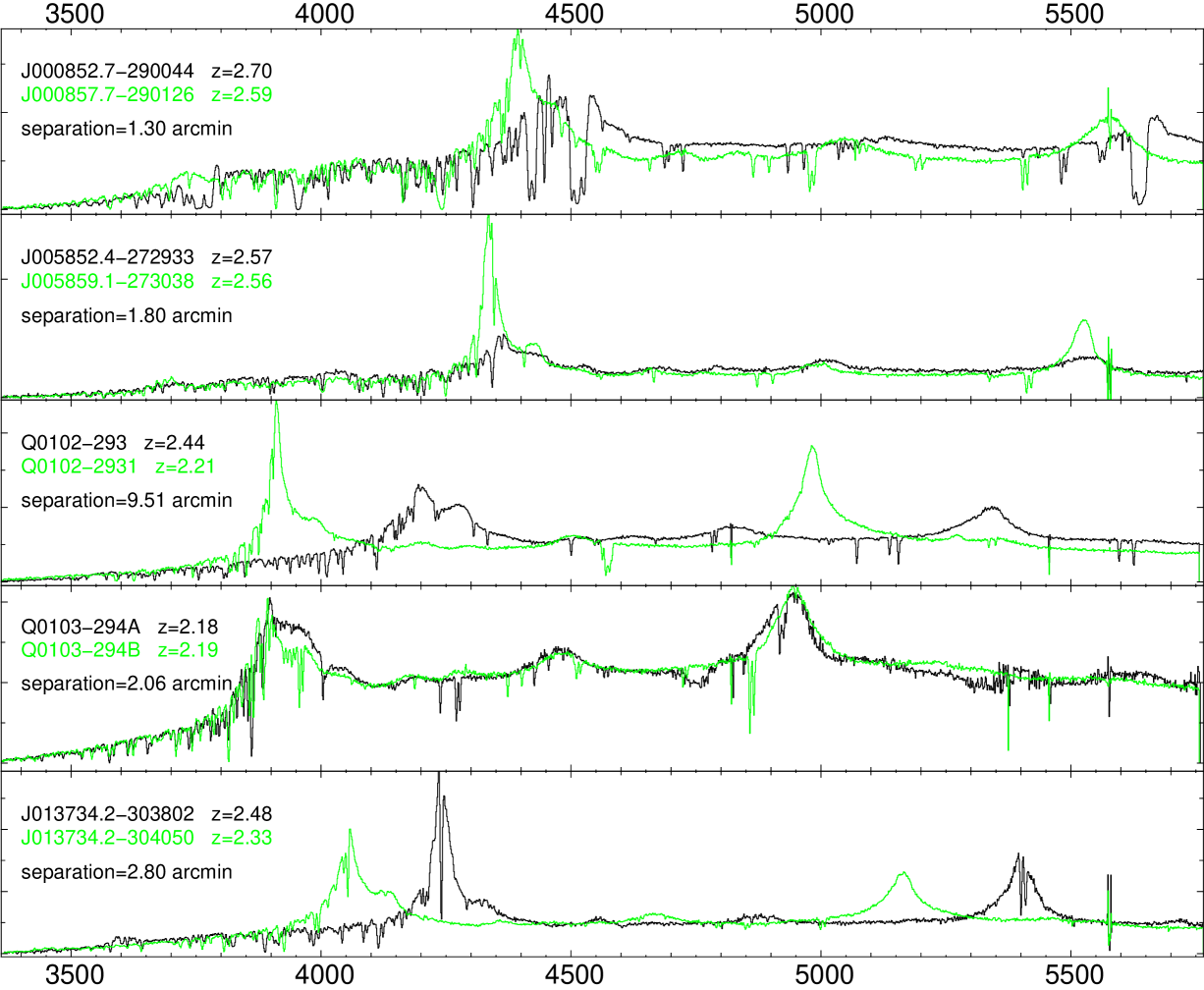
Figure 10: Spectra of the observed QSO pairs in order of increasing right ascencion. The names of the QSOs, their emission redshift and the separation between the two lines of sight are indicating in the top-left corner of each sub-panel.

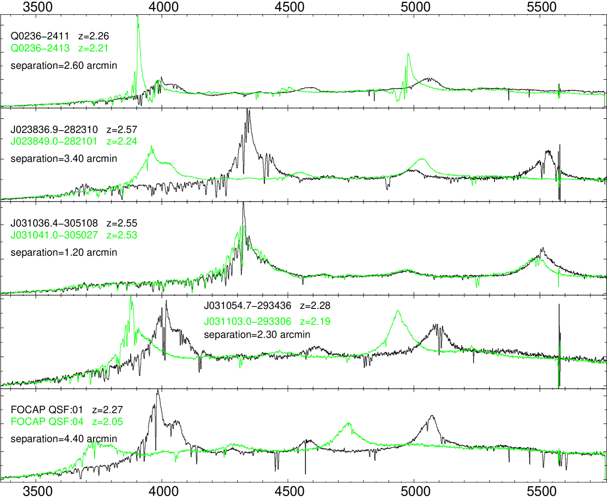
Figure 11: As in Figure C1.

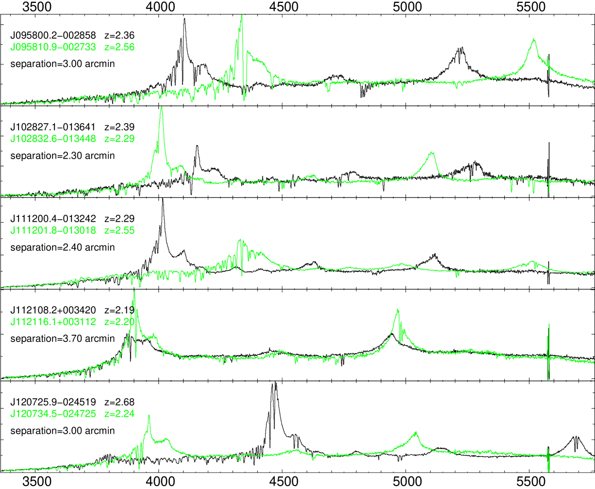
Figure 12: As in Figure C1.

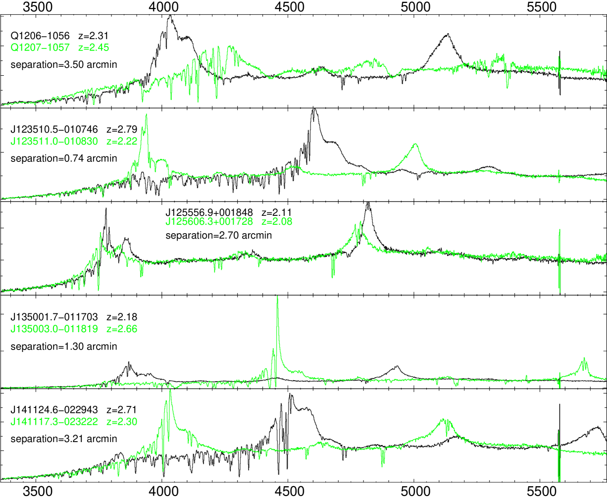
Figure 13: As in Figure C1.

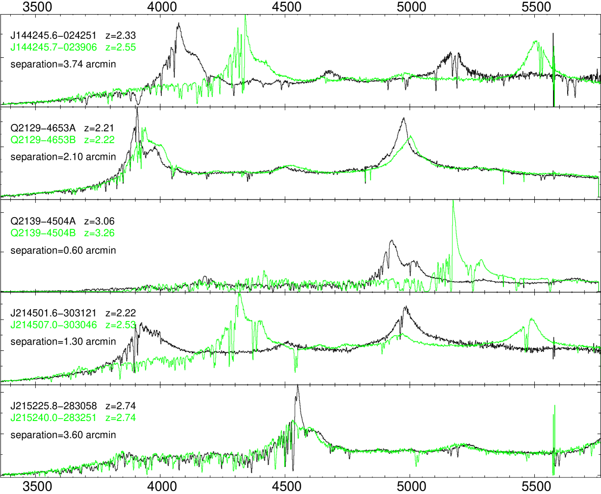
Figure 14: As in Figure C1.

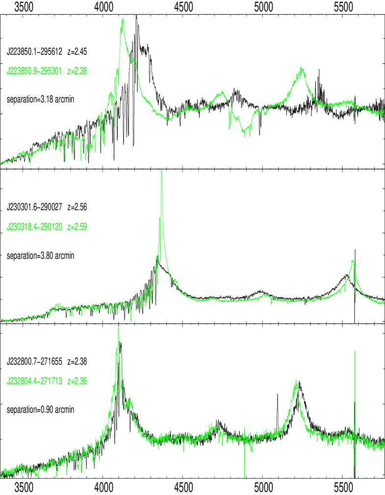
Figure 15: As in Figure C1.

References

- [1] Alcock C., & Paczyński B., 1979, Nature, 281, 358
- [2] Aracil B., Petitjean P., Smette A., Surdej J., Mücket J.P., Cristiani S., 2002, A&A, 391, 1
- [3] Aracil B., Petitjea, P., Pichon C., Bergeron J., 2004, A&A, 419, 811
- [4] Aracil B., et al., 2006, in preparation
- [5] Bechtold J., Crotts A.P.J., Duncan R.C., Fang Y., 1994, ApJ, 437, L83
- [6] Becker G., Sargent W.L.W., Rauch M., 2004, ApJ, 613, 61
- [7] Bi H., 1993, ApJ, 413, 477
- [8] Boksenberg A., Sargent W.L.W., Rauch M., 2003, astro-ph/0307557
- [9] Cen R., Miralda-Escudé J., Ostriker J.P., Rauch M., 1994, ApJ, 437, L9
- [10] Charlton J.C., Anninos P., Zhang Y., Norman M.L., 1997, ApJ, 485, 26
- [11] Chièze J.-P., Alimi J.-M., Teyssier R., 1998, ApJ, 495, 630
- [12] Croft R., Weinberg D., Bolte M., Burles S., Hernquist L., Katz N., Kirkman D., Tytler D., 2002, ApJ, 581, 20
- [13] Crotts A.P.J., Fang Y., 1998, ApJ, 502, 16
- [14] Davé R., Hernquist L., Katz N., Weinberg D.H., 1999, ApJ 511, 521
- [15] D’Odorico V., Cristiani S., D’Odorico S., Fontana A., Giallongo E., Shaver P., 1998, A&A, 339, 678
- [16] D’Odorico V., Petitjean P., Cristiani S., 2002, A&A, 390, 13
- [17] Dinshaw N., Weymann R.J., Impey C.D., Foltz C.B., Morris S.L., Ake T., 1997, ApJ, 491, 45
- [18] Dinshaw N., Impey C.D., 1996, ApJ, 458, 73
- [19] Dinshaw N., Impey C.D., Foltz C.B., Weymann R.J., Chaffee F.H., 1994, ApJ, 437, L87
- [20] Efstathiou G., Bond J. R., White S.D.M., 1992, MNRAS, 258, 1
- [21] Foltz C.B., Hewett P.C., Chaffee F.H., Hogan C.J., 1993, ApJ, 105, 22
- [22] Haardt F., Madau P., 1996, ApJ, 461, 20
- [23] Hui L., Stebbins A., Burles S., 1999, ApJ, 511, L5
- [24] Impey C.D., Foltz C.B., Petry C.E., Browne I.W.A., Patnaik A.R., 1996, ApJ, 462, L53
- [25] Jakobsen P., Perryman M.A.C., di Serego Alighieri S., Ulrich M.H., Macchetto F., 1986, ApJ, 303L, 27
- [26] Kaiser N., 1987, MNRAS, 227, 1
- [27] Lespine Y., Petitjean P., 1997, A&A, 317, 416
- [28] Mc Donald P., 2003, ApJ, 585, 34
- [29] Mc Donald P., Miralda-Escudé J., 1999, ApJ, 518, 24
- [30] McDonald P., Miralda-Escudé J., Rauch M., Sargent W.L.W., Barlow T.A., Cen R., Ostriker J.P., 2000, ApJ, 543, 1
- [31] Miralda-Escudé J., Cen R., Ostriker J.P., Rauch M., 1996, ApJ, 471, 582
- [32] Outram P.J., Hoyle F., Shanks T., 2001, MNRAS, 321, 497
- [33] Petitjean P., Mücket J.P., Kates R.E. 1995, A&A, 295, L9
- [34] Petitjean P., Rauch M., Carswell R.F., 1994, A&A, 291, 29
- [35] Petitjean P., Surdej J., Smette A., Shaver P., Mücket J., Remy M. 1998, A&A, 334, L45
- [36] Pichon C., Scannapieco E., Aracil B., Petitjean P., Aubert D., Bergeron J., Colombi S., 2003, ApJ, 597, L97, (Paper I)
- [37] Pichon C., Vergely J.L., Rollinde E., Colombi S., Petitjean P., 2001, MNRAS, 326, 597
- [38] Rauch M., Becker G.D., Viel M., Sargent W., Smette A., Simcoe R.A., Barlow T.A., Haehnelt M.G., 2005, ApJ, 632, 58
- [39] Rauch, M., Haehnelt, M. 1995, MNRAS, 275, 76
- [40] Rauch M., Sargent W.L.W., Womble D.S., Barlow T. A., 1996, ApJ, 467, L5
- [41] Rauch M, 1998, ARA&A, 36, 267
- [42] Rauch M, Sargent W.L.W., Barlow T. A., 1999, ApJ, 515, 500
- [43] Rollinde E., Petitjean P., Pichon C., 2001, A&A, 376, 28
- [44] Rollinde E., Petitjean P., Pichon C., Colombi S., Aracil B., D’Odorico V., Haehnelt M.G., 2003, MNRAS, 341, 1299
- [45] Rollinde E., Srianand R., Theuns T., Petitjean P., Chand H., 2005, MNRAS, 361, 1015
- [46] Sargent W.L.W., Boksenberg A., Steidel C.C., 1988, ApJS, 68, 539
- [47] Scannapieco E. et al. 2006, MNRAS, 365, 615
- [48] Shaver P.A., Robertson J.G., 1983, ApJ, 268, L57
- [49] Smette A., Robertson J. G., Shaver P. A., Reimers D., Wisotzki L., Koehler T., 1995, A&AS, 113, 199
- [50] Srianand R., Petitjean P., 2001, A&A, 373, 816
- [51] Sutherland R.S., Dopita M.A., 1993, ApJS, 88, 253
- [52] Teyssier R., Chièze J.-P., Alimi J.-M., 1998, ApJ, 509, 62
- [53] Theuns T., Leonard A., Efstathiou G., Pearce F.R., Thomas P.A., 1998, MNRAS, 301, 478
- [54] Viel M., Matarrese S., Mo H.J., Haehnelt M.G., Theuns T., 2002, MNRAS, 329, 848
- [55] Von Neumann J., Richmyer R.D., 1950, J. Appl. Phys., 21, 232
- [56] Weinberg D.H. et al., 1999. Proceedings of the MPA- ESO Cosmology Conference, Garching, Germany, 2-7 August 1998. Ed. A. J. Banday, R. K. Sheth, L. N. da Costa. ESO, Garching, Germany. P. 346
- [57] Williger G.M., Smette A., Hazard C., Baldwin J.A., Mc Mahon R.G., 2000, ApJ, 532, 77
- [58] Young P.A., Impey C.D., Foltz C.B., 2001, ApJ, 549, 76