Imprint of Gravitational Lensing by Population III Stars in Gamma Ray Burst Light Curves

Abstract

We propose a novel method to extract the imprint of gravitational lensing by Pop III stars in the light curves of Gamma Ray Bursts (GRBs). Significant portions of GRBs can originate in hypernovae of Pop III stars and be gravitationally lensed by foreground Pop III stars or their remnants. If the lens mass is on the order of $10^{2}-10^{3}M_{\odot}$ and the lens redshift is greater than 10, the time delay between two lensed images of a GRB is $\approx 1$s and the image separation is $\approx 10\ \mu$as. Although it is difficult to resolve the two lensed images spatially with current facilities, the light curves of two images are superimposed with a delay of $\approx 1$ s. GRB light curves usually exhibit noticeable variability, where each spike is less than 1s. If a GRB is lensed, all spikes are superimposed with the same time delay. Hence, if the autocorrelation of light curve with changing time interval is calculated, it should show the resonance at the time delay of lensed images. Applying this autocorrelation method to GRB light curves which are archived as the BATSE catalogue, we demonstrate that more than half of the light curves can show the recognizable resonance, if they are lensed. Furthermore, in 1821 GRBs we actually find one candidate of GRB lensed by a Pop III star, which may be located at redshift $20-200$. The present method is quite straightforward and therefore provides an effective tool to search for Pop III stars at redshift greater than 10. Using this method, we may find more candidates of GRBs lensed by Pop III stars in the data by the Swift satellite.

1 Introduction

The recent observation of the cosmic microwave background by Wilkinson Microwave Anisotropy Probe (WMAP) suggests that the reionization of the universe took place at redshifts of $8\lesssim z\lesssim 14$ (Spergel et al. 2003; Kogut et al. 2003; Page et al. 2006; Spergel, D., et al. 2006). This result implies that first generation stars (Pop III stars) were possibly born at $z\gtrsim 10$ if UV photons emitted from Pop III stars are responsible for cosmic reionization. However, there is no direct evidence that Pop III stars actually formed at $z>10$. Obviously, it is impossible with current or near future facilities to detect the emission from a Pop III star at such high redshifts (e.g., Mizusawa et al. 2004). But, gamma ray bursts (GRBs) can be detected even at $z>10$, if they arise there. GRBs are the only currently available tool for probing first generation objects in the universe. If one uses the data of absolute magnitude for GRBs with known redshifts, one can expect that more than half GRBs are detectable if they occur at $z>10$ (Lamb $\&$ Reichart 2000). Roughly 3000 GRBs have been detected to date, but redshifts have been measured only for 30 GRBs (Bloom et al. 2003), among which the most distant is GRB 000131 at $z=4.5$ (Andersen et al. 2000). But, if empirical relations between the spectral properties and the absolute magnitude are used, the GRBs detected to date may include events at $z>10$ (Lloyd-Ronning et al. 2002; Yonetoku et al. 2004; Murakami et al. 2005). In addition, recently a new GRB satellite, Swift, has been launched (Gehrels et al. 2004). Swift is now accumulating more data of GRBs at a high rate. Recently, GRB 050904 detected by Swift, in terms of metal absorption lines and Lyman break, turns out to have occurred at $z=6.295$ (Kawai et al. 2006).

The discovery of the association between GRB 030329 and SN 2003dh has demonstrated that at least a portion of long bursts in GRBs are caused by collapse of massive stars (Kawabata et al. 2003; Price et al. 2003; Uemura et al. 2003). On the other hand, Pop III stars are expected to form in a top-heavy fashion with the peak at $100-10^{3}M_{\odot}$ in the initial mass function (IMF) (e.g., Nakamura & Umemura 2001 and references therein). Also, the theoretical study by Heger & Woosley (2002) suggests that Pop III stars between $100M_{\odot}$ and $140M_{\odot}$ may end their lives as GRBs accompanied by the core collapse into black holes. Heger et al. (2003) estimate, assuming the IMF by Nakamura & Umemura (2001), that 5% of Pop III stars can result in GRBs. In the context of cold dark matter cosmology, more than 10-30% of GRBs are expected to occur at $z\gtrsim 10$, assuming that the redshift distributions of GRBs trace the cosmic star formation history (Bromm & Loeb 2002). Thus, observed GRBs highly probably contain GRB originating from Pop III stars at $z\gtrsim 10$.

The firm methods to measure redshifts are the detection of absorption and/or emission lines of host galaxies of GRBs (e.g., Metzger et al. 1997), or the Ly$\alpha$ absorption edge in afterglow (Andersen et al. 2000). However, these methods cannot be applied for all GRBs, but have been successful to determine redshifts only for 30 GRBs (Bloom et al. 2003). Instead, some empirical laws have been applied to much more GRBs. They include a variability-luminosity relation (Fenimore & Ramirez-Ruiz 2000), a lag-luminosity relation (Norris et al. 2000), $E_{p}$-luminosity relation (Amati et al. 2002), and the spectral peak energy-to-luminosity relation (Yonetoku et al. 2004). Applying these relations to GRBs, the redshift distributions of GRBs are derived (Fenimore & Ramirez-Ruiz 2000; Norris et al. 2000; Schaefer et al 2001; Lloyd-Ronning et al. 2002; Yonetoku et al. 2004). Some analyses conclude that a portion of GRBs are located at $z\gtrsim 10$. However, it is still controversial whether such an indirect technique is correct or not.

In this paper, we propose a novel method to constrain the redshifts of GRBs that may originate from Pop III stars at $z\gtrsim 10$. In the present method, the effects of the gravitational lensing by Pop III stars are considered. The lensing of GRBs is considered for the first time by Paczyński (1986, 1987), who proposed the possibility that a soft gamma-ray repeater is produced by gravitational lensing of a single burst at cosmological distance. Also, Loeb & Perna (1998) first discussed the microlensing effect of GRB afterglows, and Garnavich; Loeb & Stanek (2000) found the candidate microlensed afterglow (GRB 000301C). The rates of such events are further discussed from theoretical points of view (Koopmans & Wambsganss 2001; Wyithe & Turner 2002; Baltz & Hui 2005). Blaes & Webster (1992) argue the method to detect cosmological clumped dark matter by using the probability of detectable GRB lensing. Nemiroff et al. (1993) and Marani et al. (1999) search for the compact dark matter candidate using actual GRBs data obtained by the Burst and Transient Source Experiment (BATSE) satellite on the Compton Gamma Ray Observatory satellite. They focus on large mass lenses up to $10^{6}{M_{\odot}}$, which cause the delay time-scale of several tens-100 s. On the other hand, Williams & Wijers (1997) investigate the influence on GRB light curve of the millisecond gravitational lensing caused by each star in a lensing galaxy. In addition, Nemiroff & Marani (1998) argue that it is possible to place constraints on the cosmic density of dark matter, baryons, stars, and so on, by microlensing by stellar mass objects. In the present method, we focus on the gravitational lensing by Pop III stars. If the mass of Pop III stars is on the order of $10^{2}-10^{3}M_{\odot}$ and the redshift is greater than 10, the time delay between two lensed images of a GRB is $\approx 1$ s. Quite advantageously, this time delay is longer than the time resolution (64 ms) of GRB light curves and shorter than the duration of GRB events, which is several tens to 100 sec for long bursts. Thus, we can see the superimposed light curves of two lensed images. The present method seeks for the imprint of gravitational lensing by Pop III Stars in GRB light curves. We attempt to extract the imprint of lensing by calculating the autocorrelation of light curves.

In this paper, we assume a standard $\Lambda$CDM cosmological parameter: $H_{0}=70$ km $\rm{s}^{-1}$ $\rm{Mpc}^{-1}$, $\Omega_{\rm{M}}=0.3$, $\Omega_{\Lambda}=0.7$, and $\Omega_{\rm{b}}=0.04$. The paper is organized as follows: In §2, the formalism of gravitational lensing and the estimation of time delay between two images are provided. In §3, the method to find the evidence of lensing by Pop III stars is proposed. Also, we demonstrate the potentiality of the present method for artificially lensed GRBs, and describe how to determine the redshifts of lensed GRBs. In §4, we apply this method to 1821 GRB data obtained by BATSE, and find a candidate of lensed GRB. §5 is devoted to the conclusions.

2 Gravitational Lensing

We consider a GRB lensed by a foreground Pop III star. Here, we presuppose the lens model of a point mass. The Einstein ring radius gives a typical scale of gravitational lensing, which is expressed as

$$\theta_{\rm{E}}\equiv\left(\frac{4GM_{\rm{L}}}{c^{2}}\frac{D_{\rm{LS}}}{D_{\rm{OS}}D_{\rm{OL}}}\right)^{1/2},$$ (1)

where $G$ is the gravity constant, $c$ is the speed of light, $M_{\rm{L}}$ is the mass of a lens object, and $D_{\rm{LS}}$, $D_{\rm{OS}}$, and $D_{\rm{OL}}$ are respectively angular diameter distances between the lens and the source, the observer and the source, and the observer and the lens. A point mass lens produces two images with angular directions of

$$\theta=\frac{\beta}{2}\left[1\pm\sqrt{1+4\left(\frac{\theta_{\rm{E}}}{\beta}\right)^{2}}\right],$$ (2)

where $\beta$ is the angle of lens from a line-of-sight to the source. We hereafter express the image with $\theta>\theta_{\rm{E}}$ by image 1, and that with $\theta<\theta_{\rm{E}}$ by image 2. The brightness of the image 1 and the image 2 are respectively magnified by

$$A_{1,2}=\frac{1}{4}[(1+4f^{-2})^{1/2}+(1+4f^{-2})^{-1/2}\pm 2],$$ (3)

where $f=\beta/\theta_{\rm E}$. Thus, the image 1 is brighter than the original one, while the image 2 is fainter. In the case of a lens of Pop III star, the Einstein radius is estimated as

$$\theta_{\rm{E}}\simeq 10\left(\frac{M_{\rm{L}}}{10^{3}M_{\odot}}\right)^{1/2}\left(\frac{\tilde{D}}{4\times 10^{4}\rm{Mpc}}\right)^{-1/2}\mu\rm{as},$$ (4)

where $\tilde{D}\equiv D_{OS}D_{OL}/D_{LS}$. Obviously, this angular separation is impossible to resolve by current facilities. Hence, we can just observe the superposition of two images.

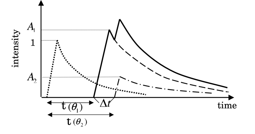
Figure 1: Schematic diagram of lensed GRB light curve. The dotted line represents the original light curve, while the dashed and dot-dashed lines represent the light curves of image 1 and image 2, respectively. The superimposed light curve of lensed images is shown by the solid line. The intensities are normalized by the maximum intensity of original light curve.

However, the light curves of two images are superimposed with a time delay caused by the gravitational lensing, as shown in Figure 1. The arrival time of signals for a lensed image is expressed as

$$t(\theta)=\frac{(1+z_{\rm{L}})}{c}\frac{D_{\rm{OS}}D_{\rm{OL}}}{D_{\rm{LS}}}\left[\frac{1}{2}(\theta-\beta)^{2}-\Psi(\theta)\right],$$ (5)

where $z_{\rm L}$ is the redshift of lens object, and $\Psi$ is so called lens potential. For the point mass lens model, $\Psi$ is expressed as

$$\Psi(\theta)=\frac{D_{\rm{LS}}}{D_{\rm{OS}}D_{\rm{OL}}}\frac{4GM_{\rm{L}}}{c^{2}}\rm{ln}|\theta/\theta_{\rm{C}}|,$$ (6)

where $\theta_{\rm{C}}$ is constant (Narayan & Bartelmann 1997). Then, the time delay between two images is given by

$$\Delta t(z_{\rm{L}},M_{\rm{L}},f)=t(\theta_{2})-t(\theta_{1})\propto M_{\rm{L}}(1+z_{\rm{L}}).$$ (7)

It should be noted that $\Delta t$ is determined solely by the mass and redshift of lens, regardless of the source redshift. In other words, the time delay places a constraint just on the lens, not on the source. However, if the lens redshift ($z_{\rm L}$) is determined, it gives the minimum value of the source redshift ($z_{\rm S}$) since $z_{\rm S}$ must be higher than $z_{\rm L}$.

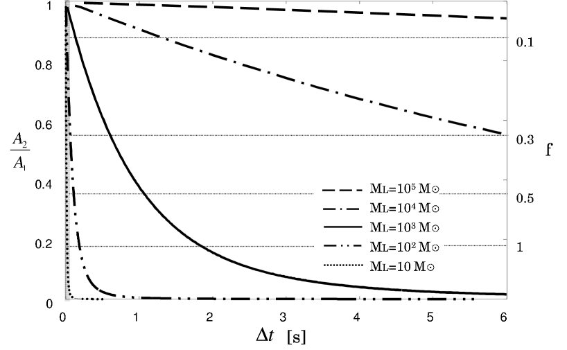
Figure 2: Relation between the time delay and the magnification ratio ($A_{2}/A_{1}$) between two images. The redshift of lens object is fixed to 50. The curves show lens masses of 10-$10^{5}M_{\rm{\odot}}$ with an increment of 1 order of magnitude. In the right vertical axis, $f=\beta/\theta_{\rm E}$, is also shown corresponding to the magnification ratio. The time resolution of BATSE data, $\Delta t=64\ \rm{ms}$, is represented by the leftmost gray region.

Fig. 2 illustrates the relation between the time delay $\Delta t$ and the magnification ratio between image 1 and image 2, assuming the lens redshift of 50. This figure shows that the lens with $\gtrsim 10^{4}M_{\odot}$ yields the time delay longer than the standard GRB duration, if the typical delay time-scale is assessed by $f\approx 1$. (Note that, as shown later, if $f$ becomes larger than unity, the ratio of magnification becomes smaller and therefore the contribution of image 2 becomes difficult to extract. Also, if $f$ becomes smaller than unity, the probability of lensing goes down. ) On the other hand, the lens with $<10M_{\odot}$ leads to $\Delta t$ shorter than the time resolution of light curves, and therefore the information of delay is buried. The mass scale of $10^{2}-10^{3}M_{\odot}$ expected for Pop III stars gives $10^{-1}\ {\rm s}\lesssim\Delta t\lesssim 1\ {\rm s}$, which is longer than the time resolution and shorter than the GRB duration. Hence, this mass range appears to be suitable for extracting the time delay information.

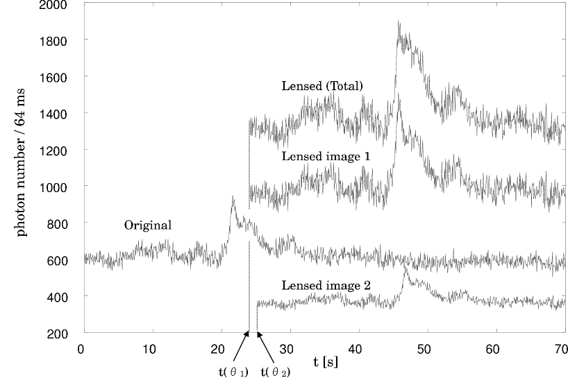
Figure 3: The original light curve of GRB 930214 obtained by BATSE and artificially lensed light curves are presented. The lens is assumed to be a Pop III star with $M_{\rm{L}}=10^{3}M_{\odot}$ at $z_{\rm{L}}=50$, while the source is located at $z_{\rm{S}}=51$. Lensed image 1, image 2, and the total light curves are shown. The time delay between two images is $\Delta t=1.0$ s under the assumption of $f=0.5$.

However, the actual GRB light curves generally exhibit variabilities with time-scale shorter than $\Delta t$. Thus, it is not straightforward to extract the time delay information. To demonstrate this difficulty, we show the light curve of GRB 930214 and the artificially lensed light curve in Figure 3, where $M_{\rm{L}}=10^{3}M_{\odot}$, $z_{\rm{L}}=50$, and $f=0.5$ are assumed. The time delay is $\Delta t=1.0$ s in this case. This figure clearly shows that if we observe only the superimposed lensed light curve, it seems impossible to recognize by appearance that this light curve is lensed. Hence, we invoke a new technique to discriminate a lensed GRB from unlensed one.

3 Autocorrelation Method

3.1 Theory

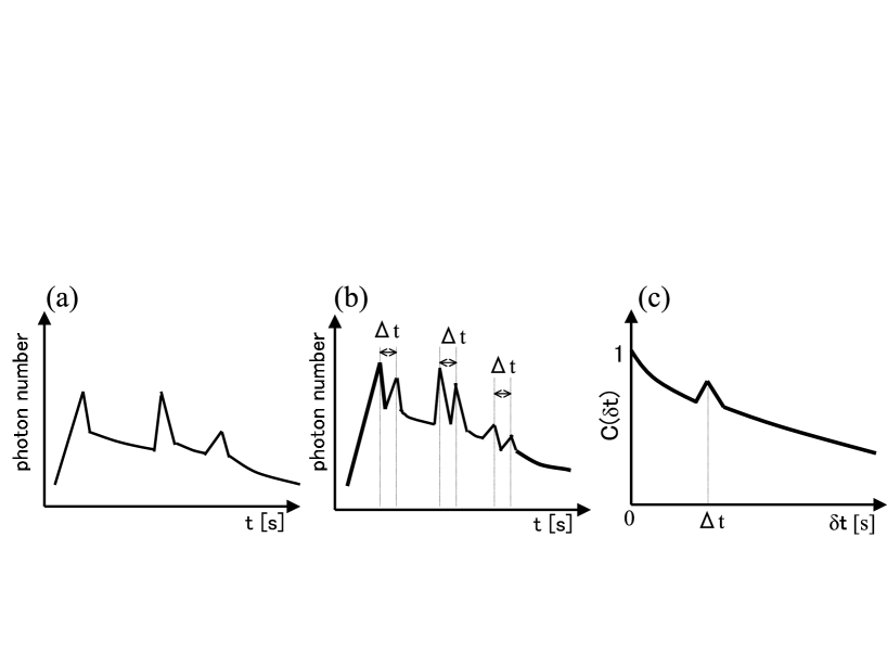
Figure 4: (a) Schematic figure of a spiky GRB light curve. (b) The light curve as the superposition of two lensed light curves with the time delay of $\Delta t$. (c) Autocorrelation function calculated for light curve (b).

We pay attention to the fact that all spikes in a light curve are individually lensed. Then, many pairs with time separation of $\Delta t$ appear in the light curve, as schematically shown in Figure 4 (b). To detect those pairs, we employ the autocorrelation method (e.g., Geiger & Schneider 1996). The autocorrelation, $C(\delta t)$, is defined as

$$C(\delta t)=\frac{\sum_{i}{I(t_{i}+\delta t)I(t_{i})}}{\sum_{i}{I(t_{i})^{2}}},$$ (8)

where $I(t_{i})$ is the number of photons contained in a i-th bin in the GRB light curve. If there are pairs with $\Delta t$, the autocorrelation (8) is expected to show the resonance “bump” around $\Delta t$, as shown in Figure 4 (c). Then, we can evaluate the time delay by the existence of this bump.

3.2 Robustness

The autocorrelation method is simple and well defined, but the issue we should check is its applicability for the actual GRB light curves. To test the robustness of this method, we produce artificially lensed light curves for GRBs in BATSE archived data, and calculate the autocorrelation. We use 1821 light curves in the BATSE catalogue with the time resolution of 64 ms . Unless otherwise specified, we adopt the data of $T_{90}$, where $T_{90}$ is defined by the duration such that the cumulative photon counts increase from 5% to 95% of the total GRB photon counts (Kouveliotou et. al. 1993, Koshut et. al. 1996). Then, the summation in equation (8) is taken in the range of $T_{90}-\delta t$. But, if the data in $T_{90}$ start with the bins whose time resolution is worse than 1024 ms, we neglect those low resolution bins.

In Figure 5, the resultant autocorrelation is shown for 10 GRB light curves. In each panel, a thin solid line represents the autocorrelation for the original light curve, while a thick solid line is the autocorrelation for the artificially lensed light curve, where $M_{\rm{L}}=10^{3}M_{\odot}$, $z_{\rm{L}}=50$, and $f=0.5$ are assumed, the same as Figure 3, and therefore the time delay of lensed images is $\Delta t=1$ s. We can see that there is no bump in $C(\delta t)$ for the original light curve, whereas a bump emerges around $\delta t=1$ s in $C(\delta t)$ for the artificially lensed light curve. Note that $C(\delta t)$ for the artificially lensed light curve is stronger than $C(\delta t)$ for all of the original light curve, owing to the amplification by gravitational lensing. $C(\delta t)$ for the artificially lensed light curve is fit by the polynomial of 8th degree. With using the best fit polynomial $F(\delta t)$, we define the dispersion, $\sigma$, of the autocorrelation curve by ${\sigma}^{2}=\sum_{j=1}^{n}[C({\delta t}_{j})-F({\delta t}_{j})]^{2}/n$, where $n$ is the number of bins. The levels of $\pm 3\sigma$ are shown by dashed lines. The zoomed view around the bump of $C(\delta t)$ for the artificially lensed light curve is also shown in each small panel. For these GRBs, bumps exceeding $3\sigma$ appear if lensed, corresponding to the time delay between two lensed images, $\Delta t$.

3.3 Dependence on $f$

In fact, not all GRB light curves exhibit bumps in $C(\delta t)$ when lensed. The fraction of GRBs which show bumps exceeding $3\sigma$ in $C(\delta t)$ depends on the value of $f=\beta/\theta_{\rm E}$. Also, the time delay $\Delta t$ and the magnification $A_{1,2}$ depend on $f$. To demonstrate this, we show the dependence on $f$ of the autocorrelation for the artificially lensed light curve of GRB 930214, in Figure 6. It is clear that if $f$ is larger, the bump is suppressed. This is because the contribution of image 2 becomes smaller with increasing $f$. In this GRB, the bump over $3\sigma$ disappears at $f>1.0$. The value of $f$ at which the bump disappears differs in each GRB. Using 220 GRB data, which are used in Fenimore & Ramirez-Ruiz (2000), we obtain the fraction of GRBs which show bumps over $3\sigma$ in $C(\delta t)$ as a function of $f$. In this analysis, $\Delta t=1.0$ s is assumed. The resultant fraction is shown in Figure 7 (a). For $f=0.5$, about a half of GRBs show bumps exceeding $3\sigma$ in $C(\delta t)$. In contrast, the cross-section of the gravitational lensing is proportional to $f^{2}$, which is also shown in Figure 7 (a). We evaluate the probability density of GRBs exhibiting bumps over $3\sigma$ by multiplying the fraction for which a bump appears by $f^{2}$. The normalized probability density against $f$ is shown in Figure 7 (b). As a result, the probability is peaked around $f=1$ and the standard deviation corresponds to $\Delta f\approx 0.25$. It is noted that this probability density is found to be hardly dependent on the value of $\Delta t$.

3.4 Optical depth

Here, we estimate the optical depth of gravitational lensing by Pop III stars. If we assume that the fraction $\alpha$ of baryonic matter composes Pop III stars at $z\geq z_{\rm{III}}$, then the optical depth is given by

$$\displaystyle\tau(z_{\rm{S}}) = \int_{z_{\rm{III}}}^{{z}_{\rm{S}}}n_{\rm{L}}(z_{\rm{L}})\sigma_{\rm{L}}\frac{cdt}{dz_{\rm{L}}}dz_{\rm{L}},$$ (9)

where $\sigma_{\rm{L}}$ is the cross-section given as $\sigma_{\rm{L}}=\pi(D_{\rm{OL}}\theta_{\rm{E}})^{2}$ and $n_{\rm{L}}(z_{\rm{L}})$ is the number density of the lens objects given as

$$n_{\rm{L}}(z_{\rm{L}})=\alpha\frac{3H_{0}^{2}}{8\pi G}\frac{\Omega_{\rm{b}}}{M_{\rm{L}}}(1+z_{\rm{L}})^{3}.$$ (10)

Then, the optical depth (9) is calculated as

$$\displaystyle\tau(z_{\rm{S}}) = \frac{3}{5}\alpha\Omega_{\rm{b}}\left\{\left[\frac{(1+z_{\rm{S}})^{5/2}+1}{(1+z_{\rm{S}})^{5/2}-1}\right]\ln(1+z_{\rm{S}})\right.$$ (11)

$$\left.\hskip 22.76228pt-\left[\frac{(1+z_{\rm{III}})^{5/2}+1}{(1+z_{\rm{III}})^{5/2}-1}\right]\ln(1+z_{\rm{III}})\right\}$$

in the Einstein-de Sitter universe (Turner, Ostriker, & Gott 1984; Turner & Umemura 1997). Here, we assume $\alpha=0.1$ and $z_{\rm{III}}=10$. The resultant optical depth of Pop III star lensing is shown in Fig. 8. Since $\tau(z_{\rm{S}})$ is the probability that a source is located inside the Einstein ring radius ($f\leq 1$), it is not the probability of bump detection. The probability of bump appearance, $p(f)$, is a decreasing function of $f$, as shown in Fig. 7 (a). Since the optical depth that $f$ is in the range of $[f,f+df]$ is given by $d\tau(z_{\rm{S}})=\tau(z_{\rm{S}})df^{2}=\tau(z_{\rm{S}})2fdf$, the probability of bump detection is given by

$$P(z_{\rm{S}})=\int_{0}^{\infty}2fp(f)\tau(z_{\rm{S}})df.$$ (12)

The resultant bump detection probability is also shown in Fig. 8. From this figure, the probability turns out to be $\approx 0.001$ for $z_{\rm{S}}=20-40$. If we take into account that more than 10-30% of GRBs occur at $z\gtrsim 10$ (Bromm & Loeb 2002), the expectation number of bump detection for lensed GRBs is assessed to be one in a few thousand GRBs.

4 A Candidate for GRB Lensed at $z\approx 60$

4.1 Data analysis

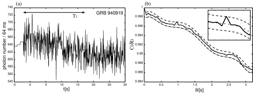
Figure 9: (a) The intrinsic light curve of GRB 940919. (b) Autocorrelation against $\delta t$. A $3\sigma$ bump appears at $\Delta t=0.96$ s.

As shown above, the autocorrelation of intrinsic light curves exhibits no bumps for almost all GRBs. But, a few in 1000 GRBs might show bumps in $C(\delta t)$ even for intrinsic light curves. Hence, we calculate the autocorrelation of all GRB light curves available in BATSE catalogue, which amount to 1821 GRBs. As a result, we have found one candidate, GRB 940919 (BATSE trigger number 3174), in which a $3\sigma$ bump in $C(\delta t)$ appears. The light curve and the autocorrelation of this GRB is shown in Figure 9. As seen in panel (b), a bump exceeding $3\sigma$ appears at $\Delta t=0.96$ s.

4.2 Statistical significance

To check the statistical significance of a bump in $C(\delta t)$ of GRB 940919, we make a test with mock light curves. Here, we generate mock light curves using a smoothed correlation function that dose not show any bump, and investigate whether bumps appear in correlation functions just from pure statistical fluctuations.

From Wiener-Kihntchine theorem, the power spectrum of light curves are given by

$$\textstyle|I(\omega)|^{2}=\mathcal{F}\left[\sum_{i}I(t_{\rm{i}})I(t_{\rm{i}}+\delta t)\right],$$ (13)

where $\mathcal{F}$ denotes the Fourier transformation and $\omega=2\pi/\delta t$. We can generate mock light curves by the inverse Fourier transformation of $I(\omega)$. Here, in order to add fluctuation to $I(\omega)$, we take random Gaussian distributions, where $|I(\omega)|$ is the standard deviation and the phase is random in the range of $[0,2\pi]$. Then, the mock light curve is given by

$$\textstyle\tilde{I}(t)=\mathcal{F}^{-1}[I(\omega)]=\sum_{\omega}|\tilde{I}(\omega)|\cos(-\phi-\omega t),$$ (14)

where $\tilde{I}(\omega)$ is a random sample in the Gaussian distribution, and $\phi$ is the random phase shift from 0 to 2$\pi$. We produce 2000 mock light curves using a correlation function, and recalculate the autocorrelation $C(\delta t)$ by equation (8). As a result, we have found that no bump higher than $3\sigma$ appears in the $C(\delta t)$ of 2000 mock light curves. A part of the recalculated $C(\delta t)$ are shown in Figure 10. Thus, it is unlikely that a bump in the correlation arises as a result of pure statistical fluctuations.

4.3 Light curve decomposition

As a further test for the lensing of GRB 940919 light curve, we attempt to decompose the light curve, assuming that it is the superposition of two lensed light curves with $\Delta t=0.96$ s, and analyze the decomposed light curves. The decomposition is made by the following recurrence formula;

$$I_{\rm{tot}}(t)=I_{1}(t)+I_{2}(t),$$ (15)

$$I_{2}(t)=\frac{A_{2}}{A_{1}}I_{1}(t-\Delta t),$$ (16)

where $I_{\rm{tot}}(t)$ is the observed intensity, and $I_{1}(t)$ and $I_{2}(t)$ are intensities for image 1 and 2, respectively. If these two equations are combined, $I_{1}(t)$ can be expressed by

$$I_{1}(t)=\sum_{j=0}^{N}\left(-\frac{A_{2}}{A_{1}}\right)^{j}I_{\rm{tot}}(t-j\Delta t).$$ (17)

The summation is taken in the range of $t-j\Delta t\geqq 0$, where $t=0$ is the starting point of $T_{90}$. Then, we can derive also $I_{2}(t)$ by equation (15). In Figure 11, the decomposed light curves are shown in the case of $f=1$ which is the most probable case as shown in §3.3. The application of this decomposition method for the finite amount of data does not guarantee that the light curve is successfully decomposed into two lensed light curves. Hence, to check the validity of this decomposition method, we calculate the cross-correlation of two decomposed light curves by

$$C_{\rm{c}}(\delta t)=\frac{\sum_{i}{I_{1}(t_{i})I_{2}(t_{i}+\delta t)}}{\sqrt{\sum_{i}{I_{1}(t_{i})^{2}}}\sqrt{\sum_{i}{I_{2}(t_{i}+\delta t)^{2}}}},$$ (18)

where $\delta t$ is the time shift. The result is shown in Figure 12. As clearly shown in this figure, the cross-correlation is peaked when $\delta t$ accords with $\Delta t=0.96$ s. Also, each decomposed light curve shows no bump higher than $3\sigma$ in the autocorrelation for a reasonable range of $f$. Hence, we can conclude that the light curve of GRB 940919 is successfully decomposed and is likely to be the superposition of two lensed light curves.

4.4 Redshift estimation

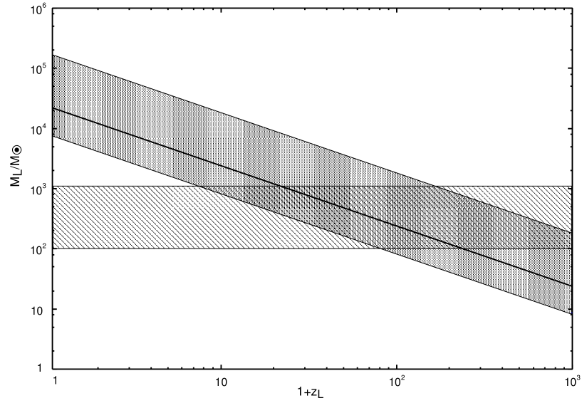
Figure 13: The dark gray region shows the suitable range of $M_{\rm{L}}(1+\rm{z_{\rm{L}}})$ for GRB 940919. Here, $3\sigma$ range of $f$ (see Fig. 7b) is adopted. The central thick solid line corresponds to the case of $f=1$, which is most probable. The hatched region is the mass range of Pop III stars by Nakamura & Umemura (2001).

Here, we constrain the redshift of the lens object. As shown in equation (7), $\Delta t$ just determines $M_{\rm{L}}(1+z_{\rm{L}})$, except for $f$. If the probability density against $f$ (Fig. 7 (b) ) is applied, we can derive a suitable range for $M_{\rm{L}}(1+z_{\rm{L}})$. The dark gray region in Figure 13 represents the suitable range for $\Delta t=0.96$ s. On the other hand, the hatched region shows the mass range of Pop III stars obtained by Nakamura & Umemura (2001). Combining these two regions, the allowed redshift of the lens object is at least $z_{\rm{L}}\approx 10$. If $f=1$ is adopted, the redshift ranges from $z_{\rm{L}}\approx 20$ to $z_{\rm{L}}\approx 200$, where the most probable one is $z_{\rm{L}}\approx 60$.

Nonetheless, there still exists another possibility that the lens object is as massive as $\sim 10^{4}M_{\odot}$ located at $z_{\rm{L}}\simeq$0, as seen in Fig. 13. Loeb (1993) and Umemura et al. (1993) suggested that relic massive black holes are candidates for such an object. Sasaki & Umemura (1996) place a constraint on $\Omega_{\rm{BH}}$ from the UV background intensity and the Gunn-Peterson effect in the context of a cold dark matter cosmology. They find that the black hole mass density might be as low as $\Omega_{\rm{BH}}/\Omega_{\rm{b}}\lesssim 10^{-3}$. Therefore, the expected number of bump detection for massive black holes is by two orders of magnitude lower than that for Pop III stars.

5 Conclusions

To place constraints on the redshifts of GRBs which originate from Pop III stars at $z>10$, we have proposed a novel method based on the gravitational lensing effects. If the lens is Pop III stars with $10^{2}-10^{3}M_{\odot}$ at $z>10$, the time delay between two lensed images of a GRB is $\approx 1$ s. This time delay is longer than the time resolution (64 ms) of GRB light curves and shorter than the duration of GRB events. Therefore, if a GRB is lensed, we observe the superposition of two lensed light curves. We have considered the autocorrelation method to extract the imprint of gravitational lensing by Pop III stars in the GRB light curves. Using BATSE data, we have derived the probability of the resonance bump in the autocorrelation function, which is an indicator for the gravitational lensing. Applying this autocorrelation method to GRB light curves in the BATSE catalogue, we have demonstrated that more than half of the light curves can show resonance bumps, if they are lensed. Furthermore, in 1821 GRB light curves, we have found one candidate of GRB lensed by a Pop III star at $z\approx 60$. The present method is quite straightforward and therefore provides an effective tool to search for Pop III stars at redshift greater than 10. Although the number of GRBs with available data is 1821 in this paper, the Swift satellite is now accumulating more GRB data. If the present method is applied for those data, more candidates for GRBs lensed at $z>10$ may be found in the future. These can provide a firm evidence of massive Pop III stars born at high redshifts.

Figure 5: Autocorrelation against $\delta t$ for 10 GRB light curves. In each panel, a thin curve shows the autocorrelation for the original light curve, while a thick curve is that for the artificially lensed light curve. Here, $M_{\rm{L}}=10^{3}M_{\odot}$, $z_{\rm{L}}=50$, and $f=0.5$ are assumed and therefore the time delay of lensed images is $\Delta t=1$ s. A dotted curve is the best fitting for the autocorrelation for lensed light curve, and two dashed curves show $\pm 3\sigma$ level from the best fitting. In each panel, a zoomed view around a correlation bump is also shown.

Figure 6: Dependence on $f=\beta/\theta_{\rm E}$ of the autocorrelation for the artificially lensed light curve of GRB 930214, which is the same GRB as panel (b) in Fig. 5. The time delay is $\Delta t=0.1$ s. The meanings of curves are the same as Fig. 5. It is seen that the bump is weaker for larger $f$.

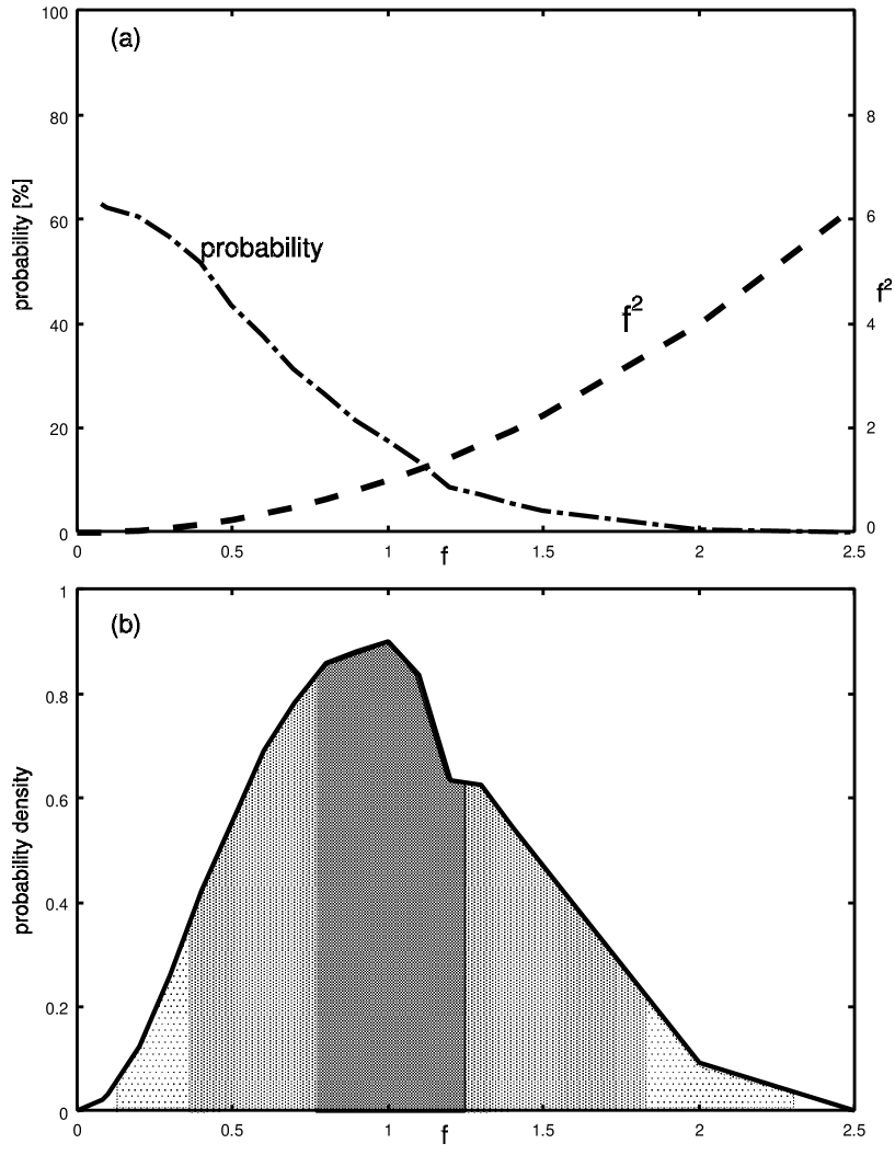
Figure 7: (a) A dot-dashed curve shows the probability of exhibiting bumps exceeding $3\sigma$. Here, $\Delta t=1.0\ \rm{s}$ is assumed. A dashed line is $f^{2}$, which is proportional to the cross-section of gravitational lens. (b) The probability density of exhibiting bumps against $f$. The gray scales represent $1\sigma$, $2\sigma$, and $3\sigma$ around $f=1$ (from dark to light).

Figure 8: Probability of bump detection for lensed GRBs, which is shown by a solid line. A dashed line is the optical depth of gravitational lensing, when a GRB as a source object is located at $z_{\rm{S}}\geq 10$ and 10% of $\Omega_{\rm{b}}$ at $z_{\rm{L}}\geq 10$ contributes to gravitational lensing as a lens object.

Figure 10: Autocorrelation for mock light curves. A thick curve is the autocorrelation for the original light curve (GRB 000421). Other thin dashed curves are a part of autocorrelations for 2000 mock light curves based on the same GRB.

Figure 11: The decomposed light curves for GRB 940919, assuming that the observed light curve is the superposition of two lensed light curves with $\Delta t=0.96$ s.

Figure 12: The cross-correlation of decomposed light curves shown in Fig. 11. A dotted line is the best fit curve, and short-dashed curves are $\pm 3\sigma$ levels. The cross-correlation shows a peak well above $3\sigma$, when $\delta t$ is the same as $\Delta t=0.96$ s.

References

- (1) Amati, L., et al. 2002, A&A, 390, 81
- (2) Andersen, M. I., et al. 2000, A&A, 364, L54
- (3) Baltz, E. A., & Hui, L. 2005, ApJ, 618, 403
- (4) Blaes, O. M., & Webster, R. L. 1992, ApJ, 391, L63
- (5) Bloom, J. S., Frail, D. A., & Kulkarni, S. R. 2003, ApJ, 594, 674
- (6) Bromm, V., & Loeb, A. 2002 ApJ, 575, 111
- (7) Fenimore, E. E., & Ramirez-Ruiz, E. 2000, astro-ph/0004176
- (8) Garnavich, P. M., Loeb, A., & Stanek, K. Z. 2000, ApJ, 544, L11
- (9) Gehrels, N., et al. 2004, ApJ, 611, 1005
- (10) Geiger, B., & Schneider, P. 1996, MNRAS, 282, 530
- (11) Heger, A., & Woosley, S. E. 2002, ApJ, 567, 532
- (12) Heger, A., et al. 2003, ApJ, 591, 288
- (13) Kawabata, K. S., et al. 2003, ApJ, 593, L19
- (14) Kawai, N. et al. 2006, Nature, 440, 184
- (15) Kogut, A., et al. 2003, ApJS, 148, 161
- (16) Koopmans, L. V. E., & Wambsganss, J. 2001, MNRAS, 325, 1317
- (17) Koshut, T. M., Paciesas, W. S., Kouveliotou, C., van Paradijs, J., Pendleton, G. N., Fishman, G.J., & Meegan, C. A. 1996, ApJ, 463, 570
- (18) Kouveliotou, C., et al. 1993, ApJ, 413, L101
- (19) Lamb, D. Q., & Reichart, D. E. 2000, ApJ, 536, 1
- (20) Lloyd-Ronning, N. M, Fryer, C. L., & Ramirez-Ruiz, E. 2002, ApJ, 574, 554
- (21) Loeb, A. 1993, ApJ, 403, 542
- (22) Loeb, A., & Perna, R. 1998, ApJ, 495, 597
- (23) Marni G. F., Nemiroff, R. J., Norris, J. P., Hurley, K., & Bonnell, J. T. 1999, ApJ, 512, L13
- (24) Metzger, M., et al. 1997, Nature, 387, 879
- (25) Mizusawa, H., Nishi, R., & Omukai, K. 2004, PASJ, 56, 487
- (26) Murakami, T., Yonetoku, D., Umemura, M., Matsubayashi, T. Yamazaki, R. 2005, ApJ, 625, L13
- (27) Nakamura, F., & Umemura, M., 2001, ApJ, 548, 19
- (28) Narayan, R., & Bartelmann, M. 1999, in Formation of Structure in the Universe, ed. A. Dekel & J. P. Ostriker (Cambridge: Cambridge Univ. Press), 360
- (29) Nemiroff, R. J., et al. 1993, ApJ, 414, 36
- (30) Nemiroff, R. J., & Marani, G.F. 1998, ApJ, 494, L173
- (31) Norris, J. P., Marani, G. F., & Bonnell, J. T. 2000, ApJ, 534, 248
- (32) Paczyński, B. 1986, ApJ, 308, L43
- (33) Paczyński, B. 1987, ApJ, 317, 51
- (34) Page, L. et al. 2006, astro-ph/0603450
- (35) Price, P. A., et al 2003, Nature, 423, 844
- (36) Sasaki, S., & Umemura, M. 1996, ApJ, 462, 104
- (37) Schaefer, B. E., Deng, M., & Band D. L. 2001, ApJ, 563, L123
- (38) Spergel, D., et al. 2003, ApJS, 148, 175
- (39) Spergel, D., et al. 2006, astro-ph/0603449
- (40) Turner, E. L., Ostriker, J. P., & Gott, J. R. 1984, ApJ, 284, 1
- (41) Turner, E. L., & Umemura, M. 1997, ApJ, 483, 603
- (42) Uemura, M., et al. 2003, Nature, 423, 843
- (43) Umemura, M., Loeb, A., & Turner, E. L. 1993, ApJ, 419, 459
- (44) Yonetoku, D., Murakami, T., Nakamura, T., Yamazaki, R., Inoue, A., K., & Ioka, K. 2004, ApJ, 609, 935
- (45) Williams, L. L. R., & Wijers, R. A. M. J. 1997, MNRAS, 286, L11
- (46) Wyithe, J. S. B., & Turner, E. L. 2002, ApJ, 575, 650