Optical Monitoring of BL Lacertae Object OJ 287:
a 40-Day Period?

Abstract

We present the results of our optical monitoring of the BL Lacertae object OJ 287 during the first half of 2005. The source did not show large-amplitude variations during this period and was in a relatively quiescent state. A possible period of 40 days was derived from its light curves in three BATC wavebands. A bluer-when-brighter chromatism was discovered, which is different from the extremely stable color during the outburst in 1994–96. The different color behaviors imply different variation mechanisms in the two states. We then re-visited the optical data on OJ 287 from the OJ-94 project and found as well a probable period of 40 days in its optical variability during the late-1994 outburst. The results suggest that two components contribute to the variability of OJ 287 during its outburst state. The first component is the normal blazar variation. This component has an amplitude similar to that of the quiescent state and also may share a similar periodicity. The second component can be taken as a ‘low-frequency modulation’ to the first component. It may be induced by the interaction of the assumed binary black holes in the center of this object. The 40-day period may be related to the helical structure of the magnetic field at the base of the jet, or to the orbital motion close to the central primary black hole.

1 INTRODUCTION

Blazars represent a peculiar subclass of active galactic nuclei (AGNs). The most prominent property of blazars is their strong and rapid variability, which is believed to originate from a relativistic jet that is pointed basically towards an observer. Another characteristic of blazars is their high polarization, with the degree and position angle also being highly variable. Superluminal motions have been observed in a significant fraction of these radio-loud flat-spectrum sources. Blazars can be classified into flat-spectrum radio quasars and BL Lac objects, depending on whether or not they show strong emission lines in their optical spectra.

Ever since the discovery of blazars and their highly variable brightness, the efforts have never stopped in searching for a periodicity in their variability. The reason for doing that is that the periodicity can put strong constraints on the emission and variation mechanisms. Although most attempts failed to find any periodicity, some positive results have been claimed for several objects (e.g., OJ 287, Sillanpää et al. 1988; 3C 345, Webb et al. 1988; 3C 120, Webb et al. 1990; S5 0716+714, Quirrenbach et al. 1991; ON 231, Liu, Xie, & Bai 1995; Mrk 421, Liu, Liu, & Xie 1997; PKS 0735+178, Fan et al. 1997; BL Lac, Fan et al. 1998; Mrk 501, Hayashida et al. 1998; AO 0235+164, Raiteri et al. 2001). However, except for the case of OJ 287, none of the claimed periods have been seen repeatedly, and they appear to be only ‘transient periods’.

The BL Lac object OJ 287 is one of the best observed blazars. It is also the only blazar that shows convincing evidence for periodic variations. By good luck and its suitable location on the sky (very close to the ecliptic where most asteroid and comet searches are made), its optical photometric measurements can be dated back to more than 100 years ago. The most prominent feature in its historical light curves is the cyclic outbursts with an interval of about 12 years, based on which Sillanpää et al. (1988) proposed a binary black hole (BBH) model for this object and predicted that a new outburst would occur in late-1994. In order to verify the predicted outburst, an international project was organized to monitor OJ 287 in multi-wavebands. This is the OJ-94 project, which covered the time range from fall 1993 to the beginning of 1997. The predicted outburst was observed with one peak at 1994.8 and another at 1996.0 (Sillanpää et al., 1996a, b). This result confirms the 12-year periodicity in the optical variability of OJ 287.

The OJ-94 project found a double-peaked structure and a quite stable color for the major outburst (Sillanpää et al., 1996a, b). Therefore, the “old” BBH model by Sillanpää et al. (1988) had to be modified, since it cannot explain the double-peaked structure. New models include the “old” hit and penetration model by Lehto & Valtonen (1996), the precessing disk/jet model by Katz (1997), and the beaming model by Villata et al. (1998). These new models also require a BBH system in the center of OJ 287, and can well explain the 12-year period, double-peaked structure of the outburst, and/or stable color (see a review by Sillanpää et al., 1996b). However, radio and polarization observations (Valtaoja et al., 2000; Pursimo et al., 2000) show that the first peak in late-1994 is a thermal flare lacking a radio counterpart, while the second peak in 1995–96 is apparently a flare dominated by synchrotron radiation and is accompanied by a radio outburst. Two previous outbursts in 1971–73 and 1983–84 also have this property. These results can not be explained by the three new models mentioned above. By incorporating the radio and polarization results, Valtaoja et al. (2000) suggested a new hit and penetration model, in which the secondary black hole hits and penetrates the accretion disk of the primary during the pericenter passage, causing a thermal flare visible only in the optical regime. At the same time, the pericenter passage enhances accretion into the primary black hole, leading to increased jet flow and formation of shocks down the jet. These become visible as simultaneous radio-optical synchrotron flares and are identified with the second optical peaks. Later, Liu & Wu (2002) derived detailed parameters of the BBH system and estimated the mass of the primary black hole as $4\times 10^{8}\,M_{\odot}$.

Alternatively, in order to explain the lack of a simultaneous radio flare in the late-1994 outburst, Marscher (1998) proposed that the late-1994 outburst comes from the base of the jet, near the central engine, while the simultaneous radio-optical flare in 1995–1996 occur in the radio core region, about a parsec down the jet. Since the base of the jet must be utterly opaque to radio emission, the first flare is not observed in radio regimes. He also mentioned that a “duty cycle” of winding up of the magnetic field at the base of the jet would also result in major quasi-periodic injection of enhanced flow into the jet (Ouyed, Pudritz, & Stone, 1997) and hence the observed periodic outbursts.

In order to re-verify the 12-year period and to evaluate the various models on OJ 287, more intensive monitoring should be carried out, not only during the outburst phases, but also in its quiescent states. We monitored OJ 287 in the first half of 2005, about 1.5 year before the predicted next outburst (Valtonen & Lehto, 1997; Kidger, 2000; Valtaoja et al., 2000; Liu & Wu, 2002). The aims are to record the variability in its quiescent state, to prepare a comparison to the variability in its outburst state, and to give more constraints to its physical model. Here we present our monitoring results and compare them with those of the 1994–96 outburst observed in the OJ-94 project. Section 2 describes our observations and data reduction procedures. The results are presented in §3, and §4 describes our re-analyses of the OJ-94 data. The physical processes responsible for the variability are discussed in §5, and a summary is given in §6.

2 OBSERVATIONS AND DATA REDUCTION

Our optical monitoring of OJ 287 was carried out on a 60/90 cm Schmidt telescope located at the Xinglong Station of the National Astronomical Observatories of China (NAOC). A Ford Aerospace $2048\times 2048$ CCD camera is mounted at its main focus. The CCD has a pixel size of $15\,\micron$ and a field of view of $58\arcmin\times 58\arcmin$, resulting in a resolution of $1\farcs 7\,\rm{pixel}^{-1}$. The telescope is equipped with a 15 color intermediate-band photometric system, covering a wavelength range from 3000 to 10,000 Å. The telescope and the photometric system are mainly used to carry out the Beijing-Arizona-Taiwan-Connecticut (BATC) survey (Zhou, 2005).

The monitoring covered the time from 2005 January 29 to April 28, or from JD 2,453,400 to 2,453,489. As a result of weather conditions and observations of other targets, there are actually 27 nights’ data in total. We used the BATC $e$, $i$, and $m$ filters. Their central wavelengths are 4885, 6685, and 8013 Å, respectively. In most nights, we made photometric measurements in only one cycle of the BATC $e$, $i$, and $m$ bands, while in a small fraction of nights, more cycles of exposures were made. The exposure times are mostly 240 s in the BATC $e$ and $m$ bands and 150 s in the $i$ band. The observational log and parameters are presented in Tables 1–3.

The procedures of data reduction include positional calibration, bias subtraction, flat-fielding, extraction of instrumental aperture magnitude, and flux calibration. The average FWHM of stellar images was about 4$\farcs$5 during our monitoring. So the radii of the aperture and the sky annulus were adopted as 5, 7, and 10 pixels (or 8$\farcs$5, 12″, and 18″) respectively during the extraction. We used the comparison stars 4, 10, and 11 in Fiorucci & Toste (1996) for the flux calibration of OJ 287. Their BATC $e$, $i$, and $m$ magnitudes are obtained by observing them and three BATC standard stars, HD 19445, HD 84937, and BD+17d4708, on a photometric night, and are listed in Table 4. Then, by comparing the instrumental magnitudes of the three comparison stars with their standard BATC magnitudes, the instrumental magnitudes of OJ 287 were calibrated into the BATC $e$, $i$, and $m$ magnitudes, and the light curves in the three BATC bands were obtained.

3 RESULTS

3.1 Light Curves

The light curves in the three BATC bands are displayed in Figure 1. Here we plot only the nightly-mean magnitudes, since the amplitudes of variations during all individual nights (if there are multi-cycles of exposures, see §2) are mostly less than 0.2 mag. The variations in the three BATC bands are basically consistent with each other. The overall amplitude was about 1.3 mag during the whole monitoring period, and the object was in a relatively quiescent state, as expected. Two cycles of variations show up in the light curves: The object varied from a minimum on JD 2,453,403 to a maximum on JD 2,453,426, and then went back to a new minimum on JD 2,453,449. With a sharp turnover, the object brightened again and reached a second maximum around JD 2,453,474. After that, the object dropped its brightness again to a third minimum on JD 2,453,489 (see also Tables 1–3). The time intervals are 46 and 40 days between the successive minima, and 48 days between the two maxima. The average is 44 days, which could be taken as the period of the variations.

One may argue that the minimum on JD 2,453,489 may not represent the actual end of the second cycle. But one can see from Figure 1 that the end parts of the light curves have very steep slopes, which implies that the object might get still fainter in magnitude, but will not spend too much in time to reach the apparent end of the second “cycle”. In other words, it appears probable that JD 2,453,489 is close to, if not actually at, the end of a second cycle.

3.2 Period of Variability

Visual inspection of the light curves in Figure 1 indicates a period of 44 days in the variations of OJ 287. In order to quantitatively derive the period, we performed a structure function (SF) analysis on the light curves. SF is frequently used to search for the typical timescales and periods in the variability (Simonetti, Cordes, & Heeschen, 1985). A characteristic timescale in a light curve, defined as the time interval between a maximum and an adjacent minimum or vice versa, is indicated by a maximum of the SF, whereas a period in the light curve causes a minimum of the SF (Smith et al., 1993; Heidt & Wagner, 1996). SF is usually calculated twice by using an interpolation algorithm, first starting from the beginning of the time series and proceeding forwards, and secondly starting from the end and proceeding backwards. This may result in two slightly different SF curves but will provide a rough assessment of the errors caused by the interpolation process.

Figure 2 shows the SF of the light curve in the BATC $i$ band. There is a deep minimum at about 44 days, which confirms the 44-day period estimated with the above visual inspection. Besides the minimum at 44 days, there is a secondary minimum around 34 days on the SF curve. It should reflect the time interval between JD 2,453,426 and JD 2,453,460, the two consecutive maxima on the light curves (while the 44-day period mainly reflects the time intervals between consecutive minima). SF curves in the other two BATC bands also show both these ‘periods’. In principle, the time intervals between any two consecutive in-phase points in a periodic light curve should be equal to each other and equal to the period. Here the difference between the two ‘periods’ may be the result of the unevenly sampled data (for example, the actual second maximum may be between JD 2,453,460 and JD 2,453,473 where we have no observations) and the relatively short time coverage of our monitoring. The two periods are expected to converge in a longer and more evenly sampled monitoring program. So here we take the mean of them, $\sim 40$ days, as the actual period in the variations.

Although both visual inspection and SF analysis indicate a period of around 40 days, it must be noted that our observations cover only two cycles of that apparent period. Moreover, in the light curves there are two gaps (JD 2,453,404–420 and JD 2,453,460–473), which may include additional maxima and/or minima. So this 40-day period needs to be confirmed with future observations, but it does lead us to search for this possible period in the earlier data. Indeed, much stronger evidence for the 40-day period was found, which will be reported in §4.

Besides the 40-day period reported here and the prominent 12-year period, Fan et al. (2002) have reported a period of 5.53 years for the optical variability of OJ 287. On shorter timescales, Efimov et al. (2002) observed an apparent period of 36.56 days for the rotation of the position angle of the optical polarization. Small fluctuations in intensity with periods of 10–20 min have also been claimed (Carrasco et al., 1985; de Diego & Kidger, 1990) but have been (at best) of a transient nature. Our 40-day period is somewhat consistent with the period reported by Efimov et al. (2002), which will be discussed later.

3.3 Spectral Behavior

Spectral behavior involved in the variability of blazars can put strong constraints on their variation mechanisms, as demonstrated by Wu et al. (2005). Optical spectral changes with brightness have been investigated for a number of blazars (e.g., Carini et al., 1992; Ghisellini et al., 1997; Speziali & Natali, 1998; Romero, Cellone, & Combi, 2000; Villata et al., 2002, 2004; Raiteri et al., 2003; Vagnetti, Trevese, & Nesci, 2003; Wu et al., 2005). Most authors have reported a bluer-when-brighter chromatism when the objects show fast flares and an achromatic trend for their long-term variability. OJ 287 was found to have an extremely stable color during the 1994–96 outburst (Sillanpää et al., 1996b). Here we investigate its spectral behavior in its relatively quiescent state.

Following Raiteri et al. (2003) and Wu et al. (2005), we use color index to denote spectral shape, and calculate the color as $e-m$ and brightness as $(e+m)/2$ for the BATC intermediate-band photometric system. As in §3.1 and §3.2, the nightly-mean magnitudes were used to calculate the colors and brightness. Figure 3 displays the color–brightness dependence. The dashed line is the best fit to the points, with the errors in both coordinates been taken into account (Press et al., 1992). The Pearson correlation coefficient is 0.504 and the significance level is 0.017. So there is a significant correlation between the brightness and color index, or in other words, there is a clear bluer-when-brighter chromatism. This is consistent with the bluer-when-brighter trend found by Vagnetti, Trevese, & Nesci (2003), but is different from the extremely stable color during the outburst in 1994–96 (Sillanpää et al., 1996b).

The different spectral behaviors between the quiescent and outburst states may indicate different variation mechanisms. In fact, in the quiescent state, the essentially simultaneous optical and radio small flares (e.g., Pursimo et al., 2000; Valtaoja et al., 2000) and the bluer-when-brighter chromatism found in this work support the hypothesis that shocks propagating along the relativistic jet and interacting with the hydrodynamically turbulent plasma and twisted magnetic field should be responsible for the variations in the quiescent state (Wagner & Witzel, 1995; Marscher, 1998). On the other hand, it is very likely that the bulk increase in brightness during the outburst state is the result of the impact of the secondary black hole onto the primary accretion disk and the subsequent enhanced accretion (Valtaoja et al., 2000), as mentioned in §1.

4 THE 1994–96 OUTBURST REVISITED

After deriving a possible period of 40 days and obtaining the properties of the variability of OJ 287 in its quiescent state, we then tried to search for new proofs to the period and compare the properties to those in the outburst state. The predicted next outburst is in 2006 (Valtonen & Lehto, 1997; Kidger, 2000; Valtaoja et al., 2000; Liu & Wu, 2002). So we at first look into the data of the outburst in 1994–96. The data on the 1994–96 outburst are from the archive of the OJ-94 project. With a visual inspection on the optical light curves of the outburst during 1994.7–1995.5 (e.g., Fig. 1 in Sillanpää et al., 1996b), we found that there were some small amplitude flares occurring at intervals of about 40 days overlaid on the prominent outburst. This is in excellent agreement with the 40-day period found in our monitoring program. We then analyzed the data in detail.

Our data analyses focused on the Johnson and Cousin $V$, $R$, and $I$ bands, which are the most densely sampled wavebands in the OJ-94 project. We at first analyzed the light curves from 1994.7 to 1995.5. In order to show the small flares more clearly, we at first made a Fast Fourier Transform (FFT) smoothing to the light curves. To have better smoothing results, the light curves were truncated at both ends where the samplings are very low. The smoothed light curves were then subtracted from the original ones, and the ‘residual light curves (or variations)’ were obtained. The procedure is illustrated in Figure 4. The large panels display the original light curves (pluses) and the smoothed ones (solid lines), while the small panels show the residual light curves. Here we carried out 240-, 100-, and 140-point FFT smoothings to the original $V$-, $R$-, and $I$-band light curves, respectively. In all three small panels, the flares can be seen clearly around JD 2,449,638, 2,449,670, 2,449,717, 2,449,752, 2,449,790, and 2,449,832. Except for the first flares, all other consecutive flares have intervals of about 40 days. The mean variation amplitude of the flares is about 1.0 mag, similar to that during the quiescent state (see §3.1).

Also notable is that there seems to be some sub-flares between the major flares mentioned above, i.e., at around JD 2,449,655, 2,449,700, 2,449,735, 2,449,775, and 2,449,817. They are weaker but somewhat broader at peaks than the major flares. The time intervals between them are also about 40 days, but, of course, the intervals between them and the neighboring major flares are about 20 days.

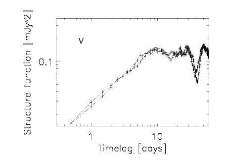
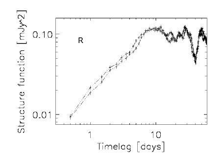
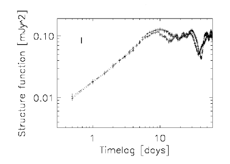
Figure 5: SFs (left) and ZDCFs (right) of the residual light curves in Fig. 4. There is a deep minimum around 40 days in all SFs, and the ZDCFs show peaks around 40, 80, and 120 days, which both indicate a period of about 40 days.

In order to derive the period quantitatively, the SFs and $z$-transformed discrete correlation functions (ZDCFs, Alexander, 1997) were calculated (in auto-correlation mode for the ZDCFs) for the residual light curves. The results are displayed in Figure 5. All three SF curves have a deep minimum at about 40 days, and all three ZDCF curves show peaks at 40, 80, and 120 days. Both indicate a period of 40 days. That is to say, the SF and ZDCF analyses confirmed the 40-day period found with visual inspections. This 40-day period is in excellent agreement with the 40-day period reported in §3.2.

We then investigated the spectral behaviors of the residual variations. Figure 6 displays the $(\Delta V-\Delta R)$ versus $\Delta V$ (left) and $(\Delta V-\Delta I)$ versus $\Delta V$ (right) distributions. As in §3, we used the nightly-mean ‘residual magnitudes’ to denote the ‘brightness’ and to calculate the ‘color’. There are strong bluer-when-brighter chromatisms in both brightness–color diagrams. The dashed lines are the linear fits to the points. The Pearson correlation coefficients are respectively 0.506 and 0.488, and the significance levels are $8.07\times 10^{-11}$ and $1.74\times 10^{-9}$, which indicate very strong correlations between the color and brightness. These bluer-when-brighter chromatisms are again in agreement with the color behavior of OJ 287 during its relatively quiescent state.

After investigating the variations of the first peak in late-1994, we then checked the data piece of the second peak in 1995–96 and those before and after the two peaks. The second peak and the data after it do not show a similar period, while the light curves before the first peak show some signs of quasi-period oscillations（QPOs). Figure 7 displays the $V$-band light curve. Flares can be seen at JD 2,449,250, 2,449,293, 2,449,327, and 2,449,366, with intervals of about 40 days. After that, the light curve is characterized by three strong sharp flares (at JD 2,449,366, 2,449,415, and 2,449,476–482) separated by three weaker but broader flares (at JD 2,449,386–397, 2,449,440–459, and 2,449,501–514), a pattern very similar to that in the late-1994 outburst. The intervals between the sharp flares is 50–60 days. Because of the unevenly sampled data and the apparently changing intervals, we do not perform a quantitative assessment to this portion of the data, but the light curves may show QPOs.

5 Physics of the 40-Day Period

That the 40-day period shows up in the variations in both quiescent and outburst states gives us new insight into the prominent outburst of OJ 287. It seems that the variation during the outburst phase can be resolved into two components. The first component is the normal blazar variation (i.e., the residual variations obtained in §4, see the smaller panels in Fig. 4). It has the similar amplitude, period, and spectral behavior as the variations in the quiescent state. The second component can be taken as a ‘low-frequency modulation’ (the solid lines in the larger panels in Fig. 4) to the first component, and may be induced by the interaction of the assumed BBHs in the center of this object (Valtaoja et al., 2000; Liu & Wu, 2002).

The variability of blazars can be best explained with the shock-in-jet model (Wagner & Witzel, 1995; Marscher, 1996), although sometimes the geometric (e.g., Wu et al., 2005) or propagative (e.g. Rickett et al., 2001) effects, or some other internal or external factors may also play a role. In the shock-in-jet model, a twisted relativistic jet originates from the central black hole and contains a hydromagnetically turbulent plasma. It undergoes fluctuations in its energy input and this causes shock waves to develop and propagate down the jet. Variability occurs when the shocks encounter fluctuations in the density of relativistic electrons, in the magnitude of the magnetic field, and in the orientation of the magnetic field.

For periodic variabilities, one usually turns to geometric origins, either a precessing jet or light house effects (e.g., Camenzind & Krockenberger, 1992; Katz, 1997; Lainela, 1999; Wu et al., 2005). However, periodic variations resulting from the geometric effects are likely to have a stable color. The bluer-when-brighter chromatisms of OJ 287 reported in §3.3 and §4 suggest that both kinds of periodic variations presented in this paper are not likely to resulted from geometric effects. Also, the fact that the variations occur in the optical regime and the presence of essentially simultaneous optical-radio small flares (Pursimo et al., 2000; Valtaoja et al., 2000) argue against a propagative origin for them.

In the first section, we have mentioned that Marscher (1998) has proposed that a “duty cycle” of winding up of the magnetic field at the base of the jet would result in major quasi-periodic injections of enhanced flow into the jet (Ouyed, Pudritz, & Stone, 1997). Here we will not discuss this possibility in accounting for the 12-year period of OJ 287. But we suggest that Marscher’s mechanism does provide a good idea for explaining the 40-day’s periodic variations of this object. In fact, Efimov et al. (2002) have observed a 36.56-day’s periodic rotation of the plane of the polarization in OJ 287, which they considered as a direct evidence for a helical magnetic field structure in the jet of this object. The 36.56-day period is consistent with our roughly 40-day period, and their observations provide a strong evidence for the scenario of winding up of magnetic field at the base of the jet.

Another possibility for explaining the 40-day period may be related to the orbital motion of the accretion disk around the central primary black hole of OJ 287. At the redshift of 0.306, the 40-day period becomes $\sim 30$ days at the rest frame of OJ 287. Adopting a mass of $4\times 10^{8}\,M_{\odot}$ for the central primary black hole (Liu & Wu, 2002), the 30-day period corresponds to the orbital motion at a radius of $r\sim 17\,r_{\rm S}$, where $r_{\rm S}$ is the Schwarzschild radius. This radius may represent the inner radius of the accretion disk and the place from which the relativistic jet originates. (For examples, according to recent numerical simulations, jets may originate from several to 100 $r_{\rm S}$, see Meier, Koide, & Uchida 2001 and Hawley & Balbus 2002.) Some disk oscillations at this radius may ‘propagate’ and be kept in the jet, and result in the observed 40-day period.

The 40-day periods both in the quiescent states and in the first peak in late-1994 can be explained with the two scenarios described above. Then why don’t we observe the 40-day period in the second peak in 1995-96? According to the models by Valtaoja et al. (2000) and Liu & Wu (2002), the structure of the inner accretion disk is undisturbed in the quiescent state and in the first peak of the major outbursts. However, when the effects of the impact of the secondary black hole onto the primary accretion disk (see §1) propagate to the base of the primary jet ($\sim 17\,r_{\rm S}$), the structure of the inner primary accretion disk and the properties (electron density, magnetic field, etc) of the primary jet are changed, and the accretion rate and hence the jet emission are significantly enhanced. Then either the periodicity is destroyed or the period changes to a new value. So we do not observe the 40-day period during the second peak of the major outburst.

After the second peak, the changed structure and properties of the primary accretion disk and jet need some time to recover to the original states (in fact, the second peak is very broad and may extend to 1997, see Fig. 2 in Pursimo et al., 2000), so the 40-day period was not observed during the 1–2 years after the second peak.

Our re-visitation of the OJ-94 data can put some constraints to the physical model of OJ 287. In the old hit and penetration model by Lehto & Valtonen (1996), the precessing disk/jet model by Katz (1997), and the beaming model by Villata et al. (1998), the two peaks of the major outbursts are resulted from the same physical processes and thus should have nearly the same behaviors. Now the 40-day period shows up in the first peak but not in the second, which gives further evidence for the assumption that the two peaks are resulted from different physical processes. In other words, our results are consistent with the models by Valtaoja et al. (2000) and Liu & Wu (2002), in which the first peak is thermal while the second is dominated by synchrotron radiation.

6 SUMMARY

During our monitoring of the BL Lac object OJ 287 in the first half of 2005, the object did not show large-amplitude variations and was in a relatively quiescent state. A possible period of 40 days was inferred from its light curves. A bluer-when-brighter chromatism was found in the variations, which is different from the overall spectral behavior during the outburst state. The different spectral behaviors indicate different variation mechanisms. The optical variability of OJ 287 during the OJ-94 project was re-visited and again a probable 40-day period was discovered. The physics responsible for the 40-day period is discussed. The 40-day period may be related to the helical structure of the magnetic field at the base of the jet, or to the orbital motion close to the central primary black hole.

Except for the 36.56-day period discovered by Efimov et al. (2002), the 40-day period has not been reported before, even though OJ 287 has been observed for more than 100 years. There are only very sparse photometric measurements before the 1972 outburst (several or even only one measurement per year). After that and till 1993, much denser monitorings were carried out but were still not sufficient to reveal our claimed period of $\sim 40$ days. The OJ-94 project, which aimed at confirming the predicted outburst in 1994 and lasted from 1993 to 1997, provided the best opportunity to find the 40-day period. The reason that no author has previously derived the 40-day period from the OJ-94 data may be that a) the focus of the OJ-94 project is on the 12-year period, and b) the methods to search for period in the variations (e.g., SF and ZDCF) cannot give correct results when the prominent overall outburst with large slope is not subtracted, as demonstrated by Smith et al. (1993) for the case of SF and illustrated in Figure 8 for the case of ZDCF.

Our monitoring revealed the 40-day period in the optical variability of OJ 287 in its quiescent state, but the duration covers only two cycles and there are two gaps in the light curves. The late-1994 outburst shows the 40-day period, but the major outbursts in 1971 and 1983 have sampling rates too low to reveal this period. Although our monitoring results and the OJ-94 data do support each other, and suggest that the 40-day period is unlikely to be a transient period, more data in both quiescent and outburst states are needed to confirm this period. Fortunately, the predicted next outburst of OJ 287 is in 2006 (Valtonen & Lehto, 1997; Kidger, 2000; Valtaoja et al., 2000; Liu & Wu, 2002). A large number of telescopes in the world will surely monitor this object around the predicted time, and we will keep on monitoring it intensively in order to confirm the 40-day period both in the quiescent and outburst states.

Figure 1: The light curves in the BATC $e$, $i$, and $m$ bands. Only nightly-mean magnitudes are plotted.

Figure 2: Structure function of the light curve in the BATC $i$ band. The minima at 34 and 44 days indicate the periods of the variation. See text for details.

Figure 3: Color index vs. brightness. The dashed line is the best fit to the points. There is a clear bluer-when-brighter chromatism.

Figure 4: Original (larger panels) and residual (smaller panels) light curves of the late-1994 outburst in the Cousins $V$, $R$, and $I$ bands, respectively. The solid curves are respectively the 240-, 100-, and 140-point FFT smoothings to the original light curves. The residuals are the differences between the originals and the smoothings.

Figure 6: The spectral behavior of the residual variations. The nightly-mean residual magnitudes are used here. The dashed lines are the best fits to the points and the correlation coefficients are respectively 0.506 and 0.488, which indicate strong correlations or strong bluer-when-brighter chromatisms.

Figure 7: The $V$-band light curve from 1993.7 to 1994.5 (data piece before the first peak). It shows some signs of QPOs. See text for details. The single point at (9356.5,14.86) is likely a false observation, so we do not take it into consideration.

Figure 8: ZDCF of the original light curve in the $R$ band in Fig. 4. Compared to the right panels of Fig. 5, the maxima at 40, 80, and 120 days is not so evident, so one can hardly extract the 40-day period from this figure.

Table 1: Observational log and results in the BATC $e$ band.

Obs. Date	Obs. Time	Julian Date	Exp. Time	$e$	$e_{\rm err}$
(yyyy mm dd)	(hh:mm:ss)		(s)	(mag)	(mag)
2005 01 29	14:57:32.0	2453400.123	300	15.671	0.144
2005 01 29	15:24:21.0	2453400.142	480	15.425	0.119
2005 01 30	16:32:48.0	2453401.189	240	15.602	0.064
2005 01 30	16:44:07.0	2453401.197	240	15.519	0.060
2005 01 30	16:58:03.0	2453401.207	240	15.525	0.057
2005 01 30	17:11:56.0	2453401.217	240	15.539	0.070
2005 01 30	17:26:02.0	2453401.226	240	15.394	0.058
2005 01 30	17:40:07.0	2453401.236	240	15.451	0.058
2005 01 30	17:53:57.0	2453401.246	240	15.497	0.061
2005 01 30	18:07:58.0	2453401.256	240	15.610	0.064
2005 01 30	18:21:47.0	2453401.265	240	15.538	0.062
2005 01 30	18:35:42.0	2453401.275	240	15.362	0.051
2005 01 30	18:49:24.0	2453401.284	240	15.431	0.055
2005 02 01	18:10:46.0	2453403.258	240	15.859	0.081
2005 02 02	13:55:03.0	2453404.080	240	15.631	0.069
2005 02 18	14:44:37.0	2453420.114	240	15.256	0.063
2005 02 19	12:48:06.0	2453421.033	240	15.066	0.058
2005 02 24	12:02:17.0	2453426.001	240	14.954	0.083
2005 02 24	12:16:13.0	2453426.011	240	14.797	0.068
2005 02 24	12:30:16.0	2453426.021	240	14.794	0.062
2005 02 24	12:44:14.0	2453426.031	240	14.926	0.074
2005 02 26	12:55:37.0	2453428.039	240	15.092	0.070
2005 02 27	13:39:46.0	2453429.069	240	15.168	0.056
2005 03 05	11:53:22.0	2453434.995	240	15.040	0.055
2005 03 06	14:17:23.0	2453436.095	300	14.697	0.124
2005 03 06	17:33:11.0	2453436.231	300	15.086	0.043
2005 03 06	17:51:14.0	2453436.244	300	15.066	0.041
2005 03 14	13:54:54.0	2453444.080	240	15.256	0.184
2005 03 15	14:19:50.0	2453445.097	240	15.409	0.076
2005 03 18	13:15:05.0	2453448.052	240	15.857	0.141
2005 03 18	13:35:35.0	2453448.066	240	15.981	0.131
2005 03 18	14:51:41.0	2453448.119	240	15.698	0.084
2005 03 18	15:05:46.0	2453448.129	240	15.542	0.083
2005 03 18	15:19:38.0	2453448.139	240	15.472	0.076
2005 03 18	15:32:58.0	2453448.148	240	15.527	0.079
2005 03 19	14:00:39.0	2453449.084	240	15.554	0.133
2005 03 19	14:14:30.0	2453449.094	240	15.620	0.158
2005 03 19	14:28:37.0	2453449.103	240	15.775	0.166
2005 03 19	14:42:45.0	2453449.113	240	16.115	0.245
2005 03 23	11:56:22.0	2453452.998	240	15.277	0.110
2005 03 26	14:08:02.0	2453456.089	240	15.007	0.097
2005 03 27	14:18:35.0	2453457.096	240	15.067	0.137
2005 03 30	11:26:04.0	2453459.976	240	14.923	0.076
2005 03 30	11:40:02.0	2453459.986	240	14.724	0.047
2005 03 30	11:54:03.0	2453459.996	240	14.822	0.049
2005 03 30	12:08:01.0	2453460.006	240	14.841	0.045
2005 03 30	12:22:07.0	2453460.015	240	14.962	0.054
2005 03 30	12:36:10.0	2453460.025	240	15.014	0.049
2005 03 30	12:50:05.0	2453460.035	240	14.924	0.053
2005 03 30	13:04:11.0	2453460.045	240	14.810	0.054
2005 04 21	12:55:57.0	2453482.039	240	15.186	0.084
2005 04 21	13:10:03.0	2453482.049	240	15.183	0.082
2005 04 22	13:24:51.0	2453483.059	240	15.547	0.125
2005 04 22	13:38:52.0	2453483.069	240	15.295	0.105
2005 04 22	13:52:31.0	2453483.078	240	15.717	0.179
2005 04 24	11:59:37.0	2453485.000	240	15.484	0.100
2005 04 24	12:13:39.0	2453485.010	240	15.822	0.123
2005 04 24	12:27:37.0	2453485.019	240	15.587	0.100
2005 04 24	12:41:45.0	2453485.029	240	15.609	0.098
2005 04 24	12:55:48.0	2453485.039	240	15.523	0.102
2005 04 28	12:47:45.0	2453489.033	240	16.140	0.144

Table 2: Observational log and results in the BATC $i$ band.

Obs. Date	Obs. Time	Julian Date	Exp. Time	$i$	$i_{\rm err}$
(yyyy mm dd)	(hh:mm:ss)		(s)	(mag)	(mag)
2005 01 29	15:02:48.0	2453400.127	180	14.637	0.048
2005 01 30	16:28:41.0	2453401.187	150	14.646	0.023
2005 01 30	16:48:34.0	2453401.200	150	14.670	0.026
2005 01 30	17:02:23.0	2453401.210	150	14.168	0.033
2005 01 30	17:16:22.0	2453401.220	150	14.661	0.024
2005 01 30	17:30:36.0	2453401.229	150	14.620	0.026
2005 01 30	17:44:21.0	2453401.239	150	14.676	0.026
2005 01 30	17:58:24.0	2453401.249	150	14.710	0.027
2005 01 30	18:12:23.0	2453401.259	150	14.697	0.026
2005 01 30	18:26:11.0	2453401.268	150	14.607	0.022
2005 01 30	18:39:56.0	2453401.278	150	14.602	0.023
2005 01 30	18:53:50.0	2453401.287	150	14.681	0.028
2005 01 31	16:56:13.0	2453402.206	150	15.070	0.058
2005 01 31	17:54:51.0	2453402.246	240	14.948	0.034
2005 02 01	18:06:20.0	2453403.254	150	15.128	0.032
2005 02 02	13:50:34.0	2453404.077	150	14.856	0.027
2005 02 18	14:33:24.0	2453420.106	150	14.454	0.026
2005 02 19	12:55:55.0	2453421.039	150	14.321	0.031
2005 02 24	12:06:44.0	2453426.005	150	14.227	0.040
2005 02 24	12:20:41.0	2453426.014	150	14.117	0.038
2005 02 24	12:34:42.0	2453426.024	150	14.200	0.043
2005 02 24	12:48:38.0	2453426.034	150	14.203	0.036
2005 02 26	13:00:04.0	2453428.042	150	14.297	0.032
2005 02 27	13:44:13.0	2453429.072	150	14.308	0.021
2005 03 05	11:43:47.0	2453434.989	150	14.514	0.040
2005 03 06	14:06:29.0	2453436.088	150	14.457	0.089
2005 03 14	13:59:20.0	2453444.083	150	14.642	0.117
2005 03 15	14:24:16.0	2453445.100	150	14.726	0.032
2005 03 18	13:19:33.0	2453448.055	150	15.028	0.131
2005 03 18	13:40:04.0	2453448.070	150	14.571	0.112
2005 03 18	14:56:06.0	2453448.122	150	14.922	0.043
2005 03 18	15:10:14.0	2453448.132	150	14.968	0.049
2005 03 18	15:23:49.0	2453448.142	150	14.893	0.046
2005 03 18	15:37:23.0	2453448.151	150	14.823	0.038
2005 03 19	14:04:53.0	2453449.087	150	14.965	0.080
2005 03 19	14:18:57.0	2453449.096	150	14.898	0.075
2005 03 19	14:33:05.0	2453449.106	150	14.935	0.075
2005 03 19	14:47:12.0	2453449.116	150	14.995	0.092
2005 03 23	12:00:49.0	2453453.000	150	14.703	0.063
2005 03 26	14:12:41.0	2453456.092	150	14.313	0.047
2005 03 27	14:13:52.0	2453457.093	150	14.218	0.054
2005 03 30	11:30:25.0	2453459.979	150	14.298	0.024
2005 03 30	11:44:28.0	2453459.989	150	14.195	0.024
2005 03 30	11:58:28.0	2453459.999	150	14.214	0.023
2005 03 30	12:12:31.0	2453460.009	150	14.208	0.023
2005 03 30	12:26:35.0	2453460.019	150	14.212	0.024
2005 03 30	12:40:32.0	2453460.028	150	14.219	0.021
2005 03 30	12:54:30.0	2453460.038	150	14.160	0.020
2005 03 30	13:08:34.0	2453460.048	150	14.151	0.022
2005 04 21	13:00:28.0	2453482.042	150	14.472	0.038
2005 04 21	13:14:26.0	2453482.052	150	14.475	0.043
2005 04 22	13:29:17.0	2453483.062	150	14.541	0.045
2005 04 22	13:43:17.0	2453483.072	150	14.617	0.047
2005 04 22	13:56:56.0	2453483.081	150	14.644	0.046
2005 04 24	12:04:30.0	2453485.003	150	14.864	0.044
2005 04 24	12:17:54.0	2453485.012	150	14.925	0.051
2005 04 24	12:32:06.0	2453485.022	150	15.052	0.052
2005 04 24	12:46:16.0	2453485.032	150	14.958	0.054
2005 04 24	13:00:12.0	2453485.042	150	14.891	0.044
2005 04 28	12:52:12.0	2453489.036	150	15.505	0.067

Table 3: Observational log and results in the BATC $m$ band.

Obs. Date	Obs. Time	Julian Date	Exp. Time	$m$	$m_{\rm err}$
(yyyy mm dd)	(hh:mm:ss)		(s)	(mag)	(mag)
2005 01 30	16:38:03.0	2453401.193	240	14.360	0.027
2005 01 30	16:52:59.0	2453401.203	240	14.259	0.028
2005 01 30	17:06:48.0	2453401.213	240	14.224	0.026
2005 01 30	17:20:50.0	2453401.223	240	14.280	0.025
2005 01 30	17:35:00.0	2453401.233	240	14.255	0.030
2005 01 30	17:48:47.0	2453401.242	240	14.330	0.029
2005 01 30	18:02:51.0	2453401.252	240	14.288	0.027
2005 01 30	18:16:35.0	2453401.261	240	14.333	0.029
2005 01 30	18:30:30.0	2453401.271	240	14.256	0.026
2005 01 30	18:44:22.0	2453401.281	240	14.271	0.028
2005 01 30	18:58:11.0	2453401.290	240	14.242	0.026
2005 01 31	18:07:54.0	2453402.255	300	14.411	0.043
2005 02 01	17:54:36.0	2453403.246	240	14.632	0.031
2005 02 02	13:45:46.0	2453404.073	240	14.542	0.035
2005 02 18	14:38:37.0	2453420.110	240	14.168	0.028
2005 02 19	13:05:40.0	2453421.046	240	13.938	0.029
2005 02 24	12:11:08.0	2453426.008	240	13.911	0.039
2005 02 24	12:25:04.0	2453426.017	240	13.866	0.044
2005 02 24	12:39:06.0	2453426.027	240	13.775	0.035
2005 02 24	12:53:01.0	2453426.037	240	13.887	0.038
2005 02 26	13:04:16.0	2453428.045	240	14.008	0.032
2005 02 27	13:48:40.0	2453429.075	240	13.979	0.023
2005 03 05	11:48:12.0	2453434.992	240	14.129	0.041
2005 03 06	14:10:55.0	2453436.091	240	14.171	0.101
2005 03 15	14:28:38.0	2453445.103	240	14.346	0.034
2005 03 18	13:30:25.0	2453448.063	240	14.696	0.092
2005 03 18	13:46:21.0	2453448.074	240	14.618	0.209
2005 03 18	14:46:31.0	2453448.116	240	14.605	0.040
2005 03 18	15:00:33.0	2453448.125	240	14.627	0.042
2005 03 18	15:14:41.0	2453448.135	240	14.493	0.050
2005 03 18	15:27:58.0	2453448.145	240	14.593	0.042
2005 03 19	14:09:20.0	2453449.090	240	14.704	0.083
2005 03 19	14:23:27.0	2453449.100	240	14.569	0.077
2005 03 19	14:37:32.0	2453449.109	240	14.675	0.075
2005 03 19	14:51:27.0	2453449.119	240	14.449	0.071
2005 03 23	12:10:44.0	2453453.008	240	14.420	0.063
2005 03 26	14:17:09.0	2453456.095	240	14.247	0.052
2005 03 27	14:08:19.0	2453457.089	240	13.949	0.046
2005 03 30	11:34:53.0	2453459.983	240	13.908	0.027
2005 03 30	11:48:55.0	2453459.992	240	13.910	0.025
2005 03 30	12:02:52.0	2453460.002	240	13.859	0.025
2005 03 30	12:16:56.0	2453460.012	240	13.886	0.023
2005 03 30	12:31:01.0	2453460.021	240	13.867	0.024
2005 03 30	12:44:57.0	2453460.031	240	13.930	0.026
2005 03 30	12:58:59.0	2453460.041	240	13.857	0.024
2005 03 30	13:13:01.0	2453460.051	240	13.882	0.026
2005 04 21	13:04:55.0	2453482.045	240	14.169	0.043
2005 04 21	13:18:51.0	2453482.055	240	14.085	0.045
2005 04 22	13:33:42.0	2453483.065	240	14.326	0.051
2005 04 22	13:47:34.0	2453483.075	240	14.173	0.045
2005 04 22	14:01:18.0	2453483.084	240	14.372	0.049
2005 04 24	12:08:38.0	2453485.006	240	14.694	0.052
2005 04 24	12:22:22.0	2453485.016	240	14.602	0.054
2005 04 24	12:36:33.0	2453485.025	240	14.429	0.043
2005 04 24	12:50:42.0	2453485.035	240	14.544	0.050
2005 04 24	13:04:26.0	2453485.045	240	14.581	0.052
2005 04 28	12:56:35.0	2453489.039	240	15.025	0.083

Table 4: BATC magnitudes of the three comparison stars

Star ID	$e$	$i$	$m$
	(mag)	(mag)	(mag)
4	14.920	14.020	13.650
10	15.010	14.510	14.280
11	15.490	14.840	14.590

References

- Alexander (1997) Alexander, T. 1997, in Astronomical Time Series, ed. D. Maoz, A. Sternberg, & E. M. Leibowitz (Dordrecht: Kluwer), 163
- Carini et al. (1992) Carini, M. T., Miller, H. R., Noble, J. C., & Goodrich, B. D. 1992, AJ, 104, 15
- Carrasco et al. (1985) Carrasco, L., Dultzin-Hacyan, D., & Cruz-Gonzalez, I. 1985, Nature, 314, 146
- Camenzind & Krockenberger (1992) Camenzind, M. & Krockenberger, M. 1992, A&A, 255, 59
- de Diego & Kidger (1990) de Diego, J. A. & Kidger, M. 1990, Ap&SS, 171, 97
- Efimov et al. (2002) Efimov, Yu. S., Shakhovskoy, N. M., Takalo, L. O., & Sillanpää, A. 2002, A&A, 381, 408
- Fan et al. (2002) Fan, J. H., Lin, R. G., Xie, G. Z., Zhang, L., Mei, D. C., Su, C. Y., & Peng, Z. M. 2002, A&A, 381, 1
- Fan et al. (1997) Fan, J. H., Xie, G. Z., Lin, R. G., Qin, Y. P., Li, K. H., & Zhang, X. 1997, A&AS, 125, 525
- Fan et al. (1998) Fan, J. H., Xie, G. Z., Pecontal, E., Pecontal, A., & Copin, Y. 1998, ApJ, 507, 173
- Fiorucci & Toste (1996) Fiorucci, M. & Tosti, G. 1996, A&AS, 116, 403
- Ghisellini et al. (1997) Ghisellini, G., Villata, M., Raiteri, C. M., et al. 1997, A&A, 327, 61
- Hawley & Balbus (2002) Hawley, J. F. & Balbus, S. A. 2002,ApJ, 573, 738
- Hayashida et al. (1998) Hayashida, N., et al. 1998, ApJ, 504, L71
- Heidt & Wagner (1996) Heidt, J. & Wagner, S. J. 1996, A&A, 305, 42
- Katz (1997) Katz, J. I. 1997, ApJ, 478, 527
- Kidger (2000) Kidger, M. R. 2000, AJ, 119, 2053
- Lainela (1999) Lainela, M., et al. 1999, ApJ, 521, 561
- Lehto & Valtonen (1996) Lehto, H. J. & Valtonen, M. J. 1996, ApJ, 460, 207
- Liu, Liu, & Xie (1997) Liu, F. K., Liu, B. F., & Xie, G. Z. 1997, A&A, 123, 569
- Liu & Wu (2002) Liu, F. K. & Wu, X. B. 2002, A&A, 338, L48
- Liu, Xie, & Bai (1995) Liu, F. K., Xie, G. Z., & Bai, J. M. 1995, A&A, 295, 1
- Marscher (1996) Marscher, A. P. 1996, in ASP Conf. Ser. 110, Blazar Continuum Variability, ed. H. R. Miller, J. R. Webb, & J. C. Nobel (San Francisco: ASP), 248
- Marscher (1998) Marscher, A. P. 1998, in Multifrequency Monitoring of Blazars (Publ. Osservatorio Astronomico Universita di Perugia), ed. G. Tosti & L. Takalo, 81
- Meier, Koide, & Uchida (2001) Meier, D. L., Koide, S. & Uchida, Y. 2001, Science, 291, 84
- Ouyed, Pudritz, & Stone (1997) Ouyed, R., Pudritz, R. E., & Stone, J. M. 1997, Nature, 385, 409
- Press et al. (1992) Press, W. H., Teukolsky, S. A., Vetterling, W. T., & Flannery, B. P. 1992, Numerical Recipes (2nd edition, Cambridge: Cambridge Univ. Press), 660
- Pursimo et al. (2000) Pursimo, T., et al. 2000, A&A, 146, 141
- Quirrenbach et al. (1991) Quirrenbach, A., et al. 1991, ApJ, 372, L71
- Raiteri et al. (2001) Raiteri, C. M., et al. 2001, A&A, 377, 396
- Raiteri et al. (2003) Raiteri, C. M., et al. 2003, A&A, 402, 151
- Rickett et al. (2001) Rickett, B. J., Witzel, A., Kraus, A., Krichbaum, T. P., & Qian, S. J. 2001, ApJ, 550, L11
- Romero, Cellone, & Combi (2000) Romero, G. E., Cellone, S. A., & Combi, J. A. 2000, AJ, 120, 1192
- Sillanpää et al. (1988) Sillanpää, A., Haarala, S., Valtonen, M. J., Sundelius, B., & Byrd, G. G. 1988, ApJ, 325, 628
- Sillanpää et al. (1996a) Sillanpää, A., et al. 1996a, A&A, 305, L17
- Sillanpää et al. (1996b) Sillanpää, A., et al. 1996b, A&A, 315, L13
- Simonetti, Cordes, & Heeschen (1985) Simonetti, J. H., Cordes, J. M., & Heeschen, D. S. 1985, ApJ, 296, 46
- Smith et al. (1993) Smith, A. G., Nair, A. D., Leacock, R. J., & Clements, D. 1993, AJ, 105, 437
- Speziali & Natali (1998) Speziali, R. & Natali, G. 1998, A&A, 339, 382
- Vagnetti, Trevese, & Nesci (2003) Vagnetti, F., Trevese, D., & Nesci, R. 2003, ApJ, 590, 123
- Valtaoja et al. (2000) Valtaoja, E., Teräsranta, H., Tornikoski, M., Sillanpää, A., Aller, M. F., Aller, H. D., & Hughes, P. A. 2000, ApJ, 531, 744
- Valtonen & Lehto (1997) Valtonen, M. J., & Lehto, H. J. 1997, ApJ, 481, L5
- Villata et al. (2002) Villata, M., et al. 2002, A&A, 390, 407
- Villata et al. (2004) Villata, M., Raiteri, C. M., Kurtanidze, O. M., et al. 2004, A&A, 421, 103
- Villata et al. (1998) Villata, M., Raiteri, C. M., Sillanpää, A., & Takalo, L. O. 1998, MNRAS, 293, L13
- Wagner & Witzel (1995) Wagner, S. J. & Witzel, A. 1995, ARA&A, 33, 163
- Webb et al. (1990) Webb, J. R. 1990, AJ, 99, 49
- Webb et al. (1988) Webb, J. R., Smith, A. G., Leacock, R. J., Fitzgibbons, G. L., Gombola, P. P., & Shepherd, D. W. 1988, AJ, 95, 374
- Wu et al. (2005) Wu, J., Peng, B., Zhou, X., Ma, J., Jiang, Z., & Chen, J. 2005, AJ, 129, 1818
- Zhou (2005) Zhou, X. 2005, JKAS, 38, 203
- Zhou et al. (2003) Zhou, X., Jiang, Z., Ma, J., Xue, S., Wu, H., Chen, J., Zhu, J., & Sun, W. 2003, A&A, 397, 361