Equation of State in Numerical Relativistic Hydrodynamics

Abstract

Relativistic temperature of gas raises the issue of the equation of state (EoS) in relativistic hydrodynamics. We study the EoS for numerical relativistic hydrodynamics, and propose a new EoS that is simple and yet approximates very closely the EoS of the single-component perfect gas in relativistic regime. We also discuss the calculation of primitive variables from conservative ones for the EoS’s considered in the paper, and present the eigenstructure of relativistic hydrodynamics for a general EoS, in a way that they can be used to build numerical codes. Tests with a code based on the Total Variation Diminishing (TVD) scheme are presented to highlight the differences induced by different EoS’s.

1 Introduction

Relativistic flows are involved in many high-energy astrophysical phenomena. Examples includes relativistic jets from Galactic sources (see Mirabel & Rodríguez, 1999, for reviews), extragalactic jets from AGNs (see Zensus, 1997, for reviews), and gamma-ray bursts (see Mészáros, 2002, for reviews). In relativistic jets from some Galactic microquasars, intrinsic beam velocities larger than $0.9c$ are typically required to explain the observed superluminal motions. In some powerful extragalactic radio sources, ejections from galactic nuclei produce true beam velocities of more than $0.98c$. In the general fireball model of gamma-ray bursts, the internal energy of gas is converted into the bulk kinetic energy during expansion and this expansion leads to relativistic outflows with high bulk Lorentz factors $\gtrsim 100$. The flow motions in these objects are usually highly nonlinear and intrinsically complex. Understanding such relativistic flows is important for correctly interpreting the observed phenomena, but often studying them is possible only through numerical simulations.

Numerical codes for special relativistic hydrodynamics (hereafter RHDs) have been successfully built, based on explicit finite difference upwind schemes that were originally developed for codes of non-relativistic hydrodynamics. These schemes utilize approximate or exact Riemann solvers and the characteristic decomposition of the hyperbolic system of conservation equations. RHD codes based on upwind schemes are able to capture sharp discontinuities robustly in complex flows, and to describe the physical solution reliably. A partial list of such codes includes the followings: Falle & Komissarov (1996) based on the van Leer scheme, Martí & Müller (1996), Aloy et al. (1999), and Mignone et al. (2005) based on the PPM scheme, Sokolov et al. (2001) based on the Godunov scheme, Choi & Ryu (2005) based on the TVD scheme, Dolezal & Wong (1995), Donat et al. (1998), DelZanna & Bucciantini (2002), and Rahman & Moore (2005) based on the ENO scheme, and Mignone & Bodo (2005) based on the HLL scheme. Reviews of some numerical approaches and test problems can be found in Martí & Müller (2003) and Wilson & Mathews (2003).

Gas in RHDs is characterized by relativistic fluid speed ($v\sim c$) and/or relativistic temperature (internal energy much greater than rest energy), and the latter brings us to the issue of the equation of state (hereafter EoS) of the gas. The EoS most commonly used in numerical RHDs, which is designed for the gas with constant ratio of specific heats, however, is essentially valid only for the gas of either subrelativistic or ultrarelativistic temperature. It is because that is not derived from relativistic kinetic theory. On the other hand, the EoS of the single-component perfect gas in relativistic regime can be derived from thermodynamics. But its form involves the modified Bessel functions (see Synge, 1957), and is too complicated to be implemented in numerical schemes.

In this paper, we study EoS for numerical RHDs. We first revisit two EoS’s previously used in numerical codes, specifically the one with constant ratio of specific heats, and the other first used by Mathews (1971) and later proposed for numerical RHDs by Mignone et al. (2005). We then propose a new EoS which is simple to be implemented in numerical codes with minimum efforts and minimum computational costs, but at the same time approximates very closely the EoS of the single-component perfect gas in relativistic regime. We also discuss the calculation of primitive variables from conservative ones for the three EoS’s. Then we present the entire eigenstructure of RHDs for a general EoS, in a way to be used to build numerical codes. In order to see the consequence of different EoS’s, shock tube tests performed with a code based on the TVD scheme are presented. The tests demonstrate the differences in flow structure due to different EoS’s. Employing a correct EoS should be important to get quantitatively correct results in problems involving a transition from non-relativistic temperature to relativistic temperature or vice versa.

This paper is organized as follows. In sections 2 and 3 we discuss three EoS’s and the calculation of primitive variables from conservative ones for those three. In sections 4 we present the eigenstructure of RHDs with a general EoS. In sections 5 and 6 we present a code based on the TVD scheme and shock tube tests with the code. Concluding remarks are drawn in section 7.

2 Relativistic Hydrodynamics

2.1 Basic Equations

The special RHD equations for an ideal fluid can be written in the laboratory frame of reference as a hyperbolic system of conservation equations

$$\frac{\partial D}{\partial t}+\frac{\partial}{\partial x_{j}}\left(Dv_{j}\right)=0,$$

$$\frac{\partial M_{i}}{\partial t}+\frac{\partial}{\partial x_{j}}\left(M_{i}v_{j}+p\delta_{ij}\right)=0,$$

$$\frac{\partial E}{\partial t}+\frac{\partial}{\partial x_{j}}\left[\left(E+p\right)v_{j}\right]=0,$$

where $D$, $M_{i}$, and $E$ are the mass density, momentum density, and total energy density, respectively (see, e.g., Landau & Lifshitz, 1959; Wilson & Mathews, 2003). The conserved quantities in the laboratory frame are expressed as

$$D=\Gamma\rho,$$

$$M_{i}=\Gamma^{2}{\rho}hv_{i},$$

$$E=\Gamma^{2}{\rho}h-p,$$

where $\rho$, $v_{i}$, $p$, and $h$ are the proper mass density, fluid three-velocity, isotropic gas pressure and specific enthalpy, respectively, and the Lorentz factor is given by

$$\Gamma=\frac{1}{\sqrt{1-v^{2}}}\qquad{\rm with}\qquad v^{2}=v_{x}^{2}+v_{y}^{2}+v_{z}^{2}.$$

In the above, the Latin indices (e.g., $i$) represents spatial coordinates and conventional Einstein summation is used. The speed of light is set to unity ($c\equiv 1$) throughout this paper.

2.2 Equation of State

The above system of equations is closed with an EoS. Without loss of generality it is given as

$$h{\equiv}h(p,\rho).$$

Then the general form of polytropic index, $n$, and the general form of sound speed, $c_{s}$, respectively can be written as

$$n={\rho}\frac{{\partial}h}{{\partial}p}-1,\qquad c_{s}^{2}=-\frac{{\rho}}{nh}\frac{{\partial}h}{{\partial}{\rho}}.$$

In addition we use a variable ${\gamma}_{h}$ to present the EoS property conveniently,

$${\gamma}_{h}=\frac{h-1}{\Theta},$$

where $\Theta=p/{\rho}$ is a temperature-like variable.

The most commonly used EoS, which is called the ideal EoS (hereafter ID), is given as

$$p=(\gamma-1)(e-\rho)\qquad{\rm or}\qquad h=1+\frac{\gamma\Theta}{\gamma-1}$$

with a constant $\gamma$. Here ${\gamma}=c_{p}/c_{v}$ is the ratio of specific heats, and $e$ is the sum of the internal and rest-mass energy densities in the local frame and is related to the specific enthalpy as

$$h=\frac{e+p}{\rho}.$$

For ID, ${\gamma}_{h}=\gamma/(\gamma-1)$ does not depend on $\Theta$. ID may be correctly applied to the gas of either subrelativistic temperature with ${\gamma}=5/3$ or ultrarelativistic temperature with ${\gamma}=4/3$. But ID is rented from non-relativistic thermodynamics, and hence it is not consistent with relativistic kinetic theory. For example, we have

$$n=\frac{1}{\gamma-1},\qquad c_{s}^{2}=\frac{\gamma\Theta(\gamma-1)}{\gamma\Theta+\gamma-1}.$$

In the high temperature limit, i.e., ${\Theta}{\rightarrow}\infty$, and for ${\gamma}>2$, $c_{s}>1$ i.e., admits superluminal sound speed. More importantly, using relativistic kinetic theory Taub (1948) showed that the choice of EoS is not arbitrary and has to satisfy the inequality,

$$(h-\Theta)(h-4\Theta)\geq 1.$$

This rules out ID for $\gamma>4/3$, if applied for $0<\Theta<\infty$.

The correct EoS for the single-component perfect gas in relativistic regime (hereafter RP) can be derived (see Synge, 1957), and is given as

$$h=\frac{K_{3}(1/\Theta)}{K_{2}(1/\Theta)},$$

where $K_{2}$ and $K_{3}$ are the modified Bessel functions of the second kind of order two and three, respectively. In the non-relativistic temperature limit ($\Theta\rightarrow 0$), $\gamma_{h}\rightarrow 5/2$, and in the ultrarelativistic temperature limit ($\Theta\rightarrow\infty$), $\gamma_{h}\rightarrow 4$. However, using the above EoS comes with a price of extra computational costs (Falle & Komissarov, 1996), since the thermodynamics of the fluid is expressed in terms of the modified Bessel functions.

There have been efforts to find approximate EoS’s which are simpler than RP but more accurate than ID. For example, Sokolov et al. (2001) proposed

$$\Theta=\frac{1}{4}\left(h-\frac{1}{h}\right)\qquad{\rm or}\qquad h=2\Theta+\sqrt{4\Theta^{2}+1}.$$

But this EoS does not satisfy either Taub’s inequality nor is consistent with the value of ${\gamma}_{h}$ in the non-relativistic temperature limit.

In a recent paper, Mignone et al. (2005) proposed for numerical RHDs an EoS that fits RP well. The EoS, which was first used by Mathews (1971), is given as

$$\frac{p}{\rho}=\frac{1}{3}\left(\frac{e}{\rho}-\frac{\rho}{e}\right)\qquad{\rm or}\qquad h=\frac{5}{2}\Theta+\frac{3}{2}\sqrt{\Theta^{2}+\frac{4}{9}},$$

and is abbreviated as TM following Mignone et al. (2005). With TM the expressions of $n$ and $c_{s}$ become

$$n=\frac{3}{2}+\frac{3}{2}\frac{\Theta}{\sqrt{\Theta^{2}+4/9}},\qquad c^{2}_{s}=\frac{5\Theta\sqrt{\Theta^{2}+4/9}+3\Theta^{2}}{12\Theta\sqrt{\Theta^{2}+4/9}+12\Theta^{2}+2}.$$

TM corresponds to the lower bound of Taub’s inequality, i.e., $(h-\Theta)(h-4\Theta)=1$. It produces the right asymptotic values for $\gamma_{h}$.

In this paper we propose a new EoS, which is a simpler algebraic function of $\Theta$ and is also a better fit of RP compared to TM. We abbreviate our proposed EoS as RC and give it by

$$\frac{p}{e-\rho}=\frac{3p+2\rho}{9p+3\rho}\qquad{\rm or}\qquad h=2\frac{6\Theta^{2}+4\Theta+1}{3\Theta+2}.$$

With RC the expressions of $n$ and $c_{s}$ become

$$n=3\frac{9\Theta^{2}+12\Theta+2}{(3\Theta+2)^{2}},\qquad c^{2}_{s}=\frac{\Theta(3\Theta+2)(18\Theta^{2}+24\Theta+5)}{3(6\Theta^{2}+4\Theta+1)(9\Theta^{2}+12\Theta+2)}.$$

RC satisfies Taub’s inequality, $(h-\Theta)(h-4\Theta)\geq 1$, for all $\Theta$. It also produces the right asymptotic values for ${\gamma}_{h}$. For both TM and RC, we have correctly $c_{s}^{2}\rightarrow 5\Theta/3$ in the non-relativistic temperature limit and $c_{s}^{2}\rightarrow 1/3$ in the ultrarelativistic temperature limit, respectively.

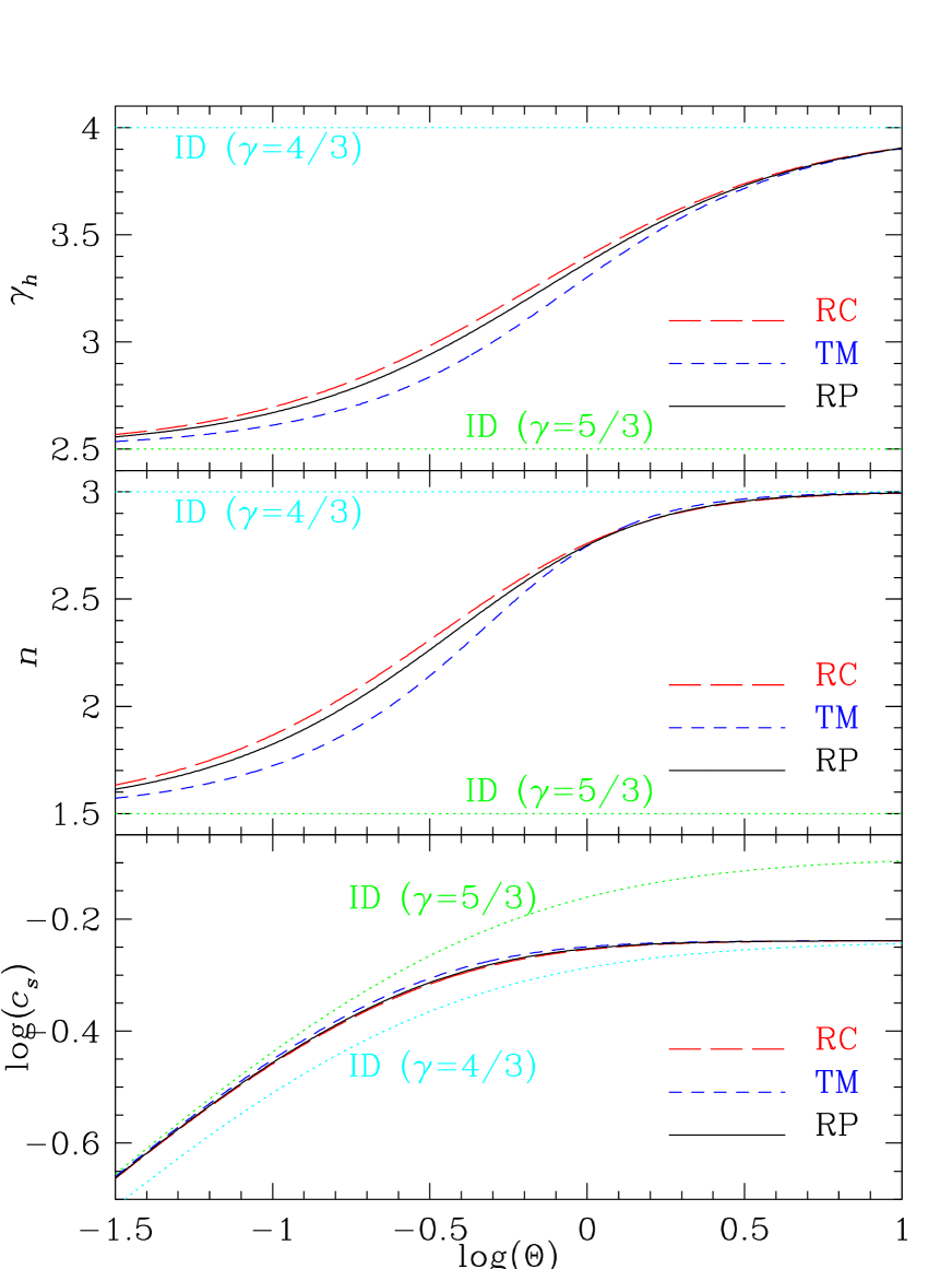
Figure 1: Comparison between different EoS’s. ${\Gamma}_{h}$, $n$, and $c_{s}$, vs $\Theta$ for RC (red-long dashed), TM (blue-short dashed), ID (green and cyan-dotted), and RP (black-solid).

In Figure 1, ${\gamma}_{h}$, $n$, and $c_{s}$ are plotted as a function of $\Theta$ to compare TM and RC to RP as well as ID. One can see that RC is a better fit of RP than TM with

$$\frac{\left|h_{\rm TM}-h_{\rm RP}\right|}{h_{\rm RP}}\lesssim 2\%,\qquad\frac{\left|h_{\rm RC}-h_{\rm RP}\right|}{h_{\rm RP}}\lesssim 0.8\%.$$

It is to be remembered that both ${\gamma}_{h}$ and $n$ are independent of $\Theta$, if ID is used.

3 Calculation of Primitive Variables

The RHD equations evolve the conserved quantities, $D$, $M_{i}$ and $E$, but we need to know the values of the primitive variables, $\rho$, $v_{i}$, $p$, to solve the equations numerically. The primitive variables can be calculated by inverting the equations (2a–2c). The equations (2a–2c) explicitly include $h$, and here we discuss the inversion for the EoS’s discussed in section 2.2, that is, ID, TM, and RC.

3.1 ID

Schneider et al. (1993) showed that the equations (2a–2c) with the EoS in (7) reduce to a single quartic equation for $v$

$$v^{4}+b_{1}v^{3}+b_{2}v^{2}+b_{3}v+b_{4}=0,$$

where

$$b_{1}=-\frac{2{\gamma}({\gamma}-1)ME}{({\gamma}-1)^{2}(M^{2}+D^{2})},\qquad b_{2}=\frac{{\gamma}^{2}E^{2}+2({\gamma}-1)M^{2}-({\gamma}-1)^{2}D^{2}}{({\gamma}-1)^{2}(M^{2}+D^{2})},$$

$$b_{3}=-\frac{2{\gamma}ME}{({\gamma}-1)^{2}(M^{2}+D^{2})},\qquad b_{4}=\frac{M^{2}}{({\gamma}-1)^{2}(M^{2}+D^{2})},$$

and $M=\sqrt{M^{2}_{x}+M^{2}_{y}+M^{2}_{z}}$. The quartic equation (18) can be solved numerically or analytically. In Choi & Ryu (2005) the analytical solution was used for the very first time, though the exact nature of the solution was not presented.

The general form of analytical roots for quartic equations can be found in Abramowitz & Stegun (1972) or on webs such as “http://mathworld.wolfram.com/QuarticEquation.html”. One may even use softwares such as Mathematica or Maxima to find the roots. We found that out of the four roots of the quartic equation (18), two are complex and two are real. The two real roots are

$$z_{1}=\frac{-B+\sqrt{B^{2}-4C}}{2},\qquad z_{2}=\frac{-B-\sqrt{B^{2}-4C}}{2},$$

where

$$B=\frac{1}{2}(b_{1}+\sqrt{b^{2}_{1}-4b_{2}+4x_{1}}),\qquad C=\frac{1}{2}(x_{1}-\sqrt{x^{2}_{1}-4b_{4}}),$$

$$x_{1}=(R+T^{\frac{1}{2}})^{\frac{1}{3}}+(R-T^{\frac{1}{2}})^{\frac{1}{3}}-\frac{a_{1}}{3},$$

$$R=\frac{9a_{1}a_{2}-27a_{3}-2a^{3}_{1}}{54},\qquad S=\frac{3a_{2}-a^{2}_{1}}{9},\qquad T=R^{2}+S^{3},$$

$$a_{1}=-b_{2},\qquad a_{2}=b_{1}b_{3}-4b_{4},\qquad a_{3}=4b_{2}b_{4}-b^{2}_{3}-b^{2}_{1}b_{4}.$$

Among the two real roots, the first one is the solution that satisfies the upper and lower limits imposed by Schneider et al. (1993), thus $v=z_{1}$. Once $v$ is found, the quantities $\rho$, $v_{i}$, $p$, are calculated by

$$\rho=\frac{D}{\Gamma},$$

$$v_{x}=\frac{M_{x}}{M}v,\qquad v_{y}=\frac{M_{y}}{M}v,\qquad v_{z}=\frac{M_{z}}{M}v,$$

$$p=(\gamma-1)[(E-M_{x}v_{x}-M_{y}v_{y}-M_{z}v_{z})-{\rho}].$$

3.2 TM

Combining the equations (2a–2c) with the EoS in (13), we get a cubic equation for $W=\Gamma^{2}-1$

$$W^{3}+c_{1}W^{2}+c_{2}W+c_{3}=0,$$

where

$$c_{1}=\frac{(E^{2}+M^{2})[4(E^{2}+M^{2})-(M^{2}+D^{2})]-14M^{2}E^{2}}{2(E^{2}-M^{2})^{2}},$$

$$c_{2}=\frac{[4(E^{2}+M^{2})-(M^{2}+D^{2})]^{2}-57M^{2}E^{2}}{16(E^{2}-M^{2})^{2}},$$

$$c_{3}=-\frac{9M^{2}E^{2}}{16(E^{2}-M^{2})^{2}}.$$

Cubic equations admit analytical solutions simpler than quartic equations (see also Abramowitz & Stegun, 1972). We found that out of the three roots of the cubic equation (23), two are unphysical giving $\Gamma<1$, and only one gives the physical solution, which is

$$W=2{\sqrt{-J}}\cos\left(\frac{\iota}{3}\right)-\frac{c_{1}}{3},$$

where

$$J=\frac{3c_{2}-c^{2}_{1}}{9},\qquad\cos{\iota}=\frac{H}{\sqrt{-J^{3}}},\qquad H=\frac{9c_{1}c_{2}-27c_{3}-2c^{3}_{1}}{54}.$$

Then the fluid speed is calculated by

$$v=\frac{W}{\sqrt{W^{2}+1}},$$

and the quantities $\rho$, $v_{i}$, $p$, are calculated by

$$\rho=\frac{D}{\Gamma}.$$

$$v_{x}=\frac{M_{x}}{M}v,\qquad v_{y}=\frac{M_{y}}{M}v,\qquad v_{z}=\frac{M_{z}}{M}v,$$

$$p=\frac{(E-M_{x}v_{x}-M_{y}v_{y}-M_{z}v_{z})^{2}-{\rho}^{2}}{3(E-M_{x}v_{x}-M_{y}v_{y}-M_{z}v_{z})}.$$

3.3 RC

Combining the equations (2a–2c) with the EoS in (15), we get

$$M\sqrt{\Gamma^{2}-1}\left[3E\Gamma(8\Gamma^{2}-1)+2D(1-4\Gamma^{2})\right]$$

$$=3\Gamma^{2}\left[4(M^{2}+E^{2})\Gamma^{2}-(M^{2}+4E^{2})\right]-2D(4E\Gamma-D)(\Gamma^{2}-1).$$

Further simplification reduces it into an equation of $8^{\rm th}$ power in $\Gamma$.

Although the equation (29) has to be solved numerically, it behaves very well. We first analyzed the nature of the roots with a root-finding routine in the IMSL library. As noted by Schneider et al. (1993), the physically meaningful solution should be between the upper limit, $\Gamma_{u}$,

$$\Gamma_{u}=\frac{1}{\sqrt{1-v^{2}_{u}}}\qquad{\rm with}\qquad v_{u}=\frac{M}{E},$$

and the lower limit, $\Gamma_{l}$, that is derived inserting $D=0$ into equation (29):

$$16(M^{2}-E^{2})^{2}\Gamma_{l}^{6}-8(M^{2}-E^{2})(M^{2}-4E^{2})\Gamma_{l}^{4}+(M^{4}-9M^{2}E^{2}+16E^{4})\Gamma_{l}^{2}+M^{2}E^{2}=0$$

(a cubic equation of $\Gamma_{l}^{2}$). Out of the eight roots of the equation (29), four are complex and four are real. Out of the four real roots, two are negative and two are positive. And out of the two real and positive roots, one is always larger than $\Gamma_{u}$, and the other is between $\Gamma_{l}$ and $\Gamma_{u}$ and so is the physical solution.

Inside RHD codes the physical solution of equation (29) can be easily calculated by the Newton-Raphson method. With an initial guess $\Gamma=\Gamma_{l}$ or any value smaller than it including 1, iteration can be proceeded upwards. Since the equation is extremely well-behaved, the iteration converges within a few steps. Once $\Gamma$ is known, the fluid speed is calculated by

$$v=\frac{\sqrt{\Gamma^{2}-1}}{\Gamma},$$

and the quantities $\rho$, $v_{i}$, $p$, are calculated by

$$\rho=\frac{D}{\Gamma}.$$

$$v_{x}=\frac{M_{x}}{M}v,\qquad v_{y}=\frac{M_{y}}{M}v,\qquad v_{z}=\frac{M_{z}}{M}v$$

$$p=\frac{(E-M_{i}v_{i})-2\rho+\left[(E-M_{i}v_{i})^{2}+4\rho(E-M_{i}v_{i})-4\rho^{2}\right]^{\frac{1}{2}}}{6},$$

where

$$M_{i}v_{i}=M_{x}v_{x}+M_{y}v_{y}+M_{z}v_{z}.$$

4 Eigenvalues and Eigenvectors

In building a code based on the Roe-type schemes such as the TVD and ENO schemes that solves a hyperbolic system of conservation equations, the eigenstructure (eigenvalues and eigenvectors of the Jacobian matrix) is required. The Eigenstructure for RHDs was previously described, for instance, in Donat et al. (1998). However, with the parameter vector different from that of Donat et al. (1998), the eigenvectors become different. Here we present our complete set of eigenvalues and eigenvectors without assuming any particular form of EoS.

Equations (1a)–(1c) can be written as

$$\frac{\partial\vec{q}}{\partial t}+\frac{\partial\vec{F}_{j}}{\partial x_{j}}=0$$

with the state and flux vectors

$$\vec{q}=\left[\matrix{D\cr M_{i}\cr E}\right],\qquad\vec{F}_{j}=\left[\matrix{Dv_{j}\cr M_{i}v_{j}+p\delta_{ij}\cr\left(E+p\right)v_{j}}\right],$$

or as

$$\frac{\partial\vec{q}}{\partial t}+A_{j}\frac{\partial\vec{q}}{\partial x_{j}}=0,\qquad A_{j}=\frac{\partial\vec{F}_{j}}{\partial\vec{q}}.$$

Here $A_{j}$ is the $5\times 5$ Jacobian matrix composed with the state and flux vectors. The construction of the matrix $A_{j}$ can be simplified by introducing a parameter vector, $\vec{u}$, as

$$A_{j}=\frac{\partial\vec{F}_{j}}{\partial\vec{u}}\frac{\partial\vec{u}}{\partial\vec{q}}.$$

We choose the vector made of primitive variables as the parameter vector

$$\vec{u}=\left[\matrix{\rho\cr v_{i}\cr p}\right].$$

4.1 One Velocity Component

The eigenstructure is simplified if only a single component of velocity is chosen, i.e., $v=v_{x}$. In principle it can be reduced from that with three components of velocity in the next subsection. Nevertheless we present it, for the case that the simpler eigenstructure with one velocity component can be used.

The explicit form of the Jacobian matrix, $A$, is presented in Appendix A. The eigenvalues of $A$ are,

$$a_{-}=\frac{v-c_{s}}{1-c_{s}v},\qquad a_{o}=v,\qquad a_{+}=\frac{v+c_{s}}{1+c_{s}v}.$$

The right eigenvectors are

$$\vec{R}_{-}=\left[\matrix{1\cr\Gamma h(v-c_{s})\cr\Gamma h(1-c_{s}v)}\right],\qquad\vec{R}_{0}=\left[\matrix{1\cr\Gamma hv(1-nc^{2}_{s})\cr\Gamma h(1-nc^{2}_{s})}\right],\qquad\vec{R}_{+}=\left[\matrix{1\cr\Gamma h(v+c_{s})\cr\Gamma h(1+c_{s}v)}\right].$$

and the left eigenvectors are

$$\vec{L}_{-}=-\frac{1}{2hnc^{2}_{s}}\left[h(1-nc^{2}_{s}),~{}~{}\Gamma(v+nc_{s}),~{}~{}-\Gamma(1+nc_{s}v)\right],$$

$$\vec{L}_{0}=\frac{1}{hnc^{2}_{s}}\left[h,~{}~{}\Gamma v,~{}~{}-\Gamma\right],$$

$$\vec{L}_{+}=-\frac{1}{2hnc^{2}_{s}}\left[h(1-nc^{2}_{s}),~{}~{}\Gamma(v-nc_{s}),~{}~{}-\Gamma(1-nc_{s}v)\right].$$

Here $n$ and $c_{s}$ are given in equation (5).

4.2 Three Velocity Components

The $x$-component of the Jacobian matrix, $A_{x}$, when all the three components of velocity are considered, is presented in Appendix B. The eigenvalues of $A_{x}$ are

$$a_{1}=\frac{\left(1-c_{s}^{2}\right)v_{x}-c_{s}/\Gamma\cdot\sqrt{Q}}{1-c_{s}^{2}v^{2}},$$

$$a_{2}=v_{x},$$

$$a_{3}=v_{x},$$

$$a_{4}=v_{x},$$

$$a_{5}=\frac{\left(1-c_{s}^{2}\right)v_{x}+c_{s}/\Gamma\cdot\sqrt{Q}}{1-c_{s}^{2}v^{2}},$$

where $Q=1-v^{2}_{x}-c^{2}_{s}(v^{2}_{y}+v^{2}_{z})$. The eigenvalues represent the five characteristic speeds associated with two sound wave modes ($a_{1}$ and $a_{5}$) and three entropy modes ($a_{2}$, $a_{3}$, and $a_{4}$). A remarkable feature is that the eigenvalues do not explicitly depend on $h$ and $n$, but only on $v_{i}$ and $c_{s}$. Hence the eigenvalues are the same regardless of the choice of EoS once the sound speed is defined properly.

The corresponding right eigenvectors ($A_{x}\vec{R}=a\vec{R}$), however, depends explicitly on $h$ and $n$, and the complete set is given by

$$\vec{R}_{1}=\left[\frac{1-a_{1}v_{x}}{\Gamma},~{}~{}a_{1}h(1-v^{2}_{x}),~{}~{}h(1-a_{1}v_{x})v_{y},~{}~{}h(1-a_{1}v_{x})v_{z},~{}~{}h(1-v^{2}_{x})\right]^{\mathrm{T}},$$

$$\vec{R}_{2}={\tilde{X}}\left[X_{1},~{}~{}X_{2},~{}~{}X_{3},~{}~{}X_{4},~{}~{}X_{5}\right]^{\mathrm{T}},$$

$$\vec{R}_{3}=\frac{1}{1-v^{2}_{x}}\left[\frac{v_{y}}{\Gamma h},~{}~{}2v_{x}v_{y},~{}~{}1-v^{2}_{x}+v^{2}_{y},~{}~{}v_{y}v_{z},~{}~{}2v_{y}\right]^{\mathrm{T}},$$

$$\vec{R}_{4}=\frac{1}{1-v^{2}_{x}}\left[\frac{v_{z}}{\Gamma h},~{}~{}2v_{x}v_{z},~{}~{}v_{y}v_{z},~{}~{}1-v^{2}_{x}+v^{2}_{z},~{}~{}2v_{z}\right]^{\mathrm{T}},$$

$$\vec{R}_{5}=\left[\frac{1-a_{5}v_{x}}{\Gamma},~{}~{}a_{5}h(1-v^{2}_{x}),~{}~{}h(1-a_{5}v_{x})v_{y},~{}~{}h(1-a_{5}v_{x})v_{z},~{}~{}h(1-v^{2}_{x})\right]^{\mathrm{T}},$$

where

$$X_{1}=\frac{nc^{2}_{s}(v^{2}_{y}+v^{2}_{z})+(1-v^{2}_{x})}{\Gamma h},$$

$$X_{2}=\left[2nc^{2}_{s}(v^{2}_{y}+v^{2}_{z})+(1-nc^{2}_{s})(1-v^{2}_{x})\right]v_{x},$$

$$X_{3}=\left[nc^{2}_{s}(v^{2}_{y}+v^{2}_{z})+(1-v^{2}_{x})\right]v_{y},$$

$$X_{4}=\left[nc^{2}_{s}(v^{2}_{y}+v^{2}_{z})+(1-v^{2}_{x})\right]v_{z},$$

$$X_{5}=2nc^{2}_{s}(v^{2}_{y}+v^{2}_{z})+(1-nc^{2}_{s})(1-v^{2}_{x}).$$

$${\tilde{X}}=\frac{{\Gamma}^{2}}{nc^{2}_{s}(1-v^{2}_{x})},$$

The complete set of the left eigenvectors ($\vec{L}A_{x}=a\vec{L}$), which are orthonormal to the right eigenvectors, is

$$\vec{L}_{1}=\frac{1}{\tilde{Y}}_{1}\left[Y_{11},~{}~{}Y_{12},~{}~{}Y_{13},~{}~{}Y_{13},~{}~{}Y_{15}\right],$$

$$\vec{L}_{2}=\left[\frac{h}{\Gamma},~{}~{}v_{x},~{}~{}v_{y},~{}~{}v_{z},~{}~{}-1\right],$$

$$\vec{L}_{3}=\left[-{\Gamma}hv_{y},~{}~{}0,~{}~{}1,~{}~{}0,~{}~{}0\right],$$

$$\vec{L}_{4}=\left[-{\Gamma}hv_{z},~{}~{}0,~{}~{}0,~{}~{}1,~{}~{}0\right],$$

$$\vec{L}_{5}=\frac{1}{\tilde{Y}}_{5}\left[Y_{51},~{}~{}Y_{52},~{}~{}Y_{53},~{}~{}Y_{53},~{}~{}Y_{55}\right],$$

where

$$Y_{i1}=-\frac{h}{\Gamma}(1-a_{i}v_{x})(1-nc^{2}_{s}),$$

$$Y_{i2}=na_{i}(1-c^{2}_{s}v^{2})+a_{i}(1+nc^{2}_{s})v^{2}_{x}-(1+n)v_{x},$$

$$Y_{i3}=-(1+nc^{2}_{s})(1-a_{i}v_{x})v_{y},$$

$$Y_{i4}=-(1+nc^{2}_{s})(1-a_{i}v_{x})v_{z},$$

$$Y_{i5}=(1+nc^{2}_{s}v^{2})+(1-c^{2}_{s})nv^{2}_{x}-a_{i}(1+n)v_{x},$$

$${\tilde{Y}}_{i}=hn\left[(a_{i}-v_{x})^{2}Q+\frac{c^{2}_{s}}{\Gamma^{2}}\right],$$

and index $i=1,\ 5$.

We note that with three degenerate modes that have same eigenvalues, $a_{2}=a_{3}=a_{4}$, we have a freedom to write down the right and left eigenvectors in a variety of different forms. We chose to present the ones that produce the best results with the TVD code described next.

5 One-Dimensional Functioning Code

To be used for demonstration of the differences in flow structure due to different EoS’s, a one-dimensional functioning code based on the Total Variation Diminishing (TVD) scheme was built. The code utilizes the eigenvalues and eigenvectors given in the previous section, and can employ arbitrary EoS’s including those in section 2.2.

5.1 The TVD Scheme

The TVD scheme, originally developed by Harten (1983), is an Eulerian, finite-difference scheme with second-order accuracy in space and time. The second-order accuracy in time is achieved by modifying numerical flux using the quantities in five grid cells (see below and Harten, 1983, for details). The scheme is basically identical to that previously used in Ryu et al. (1993) and Choi & Ryu (2005). But for completeness, the procedure is concisely shown here.

The state vector $\vec{q}_{i}^{n}$ at the cell center $i$ at the time step $n$ is updated by calculating the modified flux vector $\bar{\vec{f}}_{x,i\pm 1/2}$ along the $x$-direction at the cell interface $i\pm 1/2$ as follows:

$$L_{x}\vec{q}_{i}^{n}=\vec{q}_{i}^{n}-\frac{\Delta t^{n}}{\Delta x}\left(\bar{\vec{f}}_{x,i+1/2}-\bar{\vec{f}}_{x,i-1/2}\right),$$

$$\bar{\vec{f}}_{x,i+1/2}=\frac{1}{2}\left[\vec{F}_{x}(\vec{q}_{i}^{n})+\vec{F}_{x}(\vec{q}_{i+1}^{n})\right]-\frac{\Delta x}{2\Delta t^{n}}\sum_{k=1}^{5}\beta_{k,i+1/2}\vec{R}_{k,i+1/2}^{n},$$

$$\beta_{k,i+1/2}=Q_{k}(\frac{\Delta t^{n}}{\Delta x}a_{k,i+1/2}^{n}+\gamma_{k,i+1/2})\alpha_{k,i+1/2}-\left(g_{k,i}+g_{k,i+1}\right),$$

$$\gamma_{k,i+1/2}=\left\{\begin{array}[]{lcl}\left(g_{k,i+1}-g_{k,i}\right)/\alpha_{k,i+1/2}&\mathrm{for}&\alpha_{k,i+1/2}\neq 0,\\ 0&\mathrm{for}&\alpha_{k,i+1/2}=0,\end{array}\right.$$

$$g_{k,i}=\mathrm{sign}(\tilde{g}_{k,i+1/2})\mathrm{max}\{0,\mathrm{min}[|\tilde{g}_{k,i+1/2}|,\mathrm{sign}(\tilde{g}_{k,i+1/2})\tilde{g}_{k,i-1/2}]\},$$

$$g_{k,i}=\mathrm{sign}(\tilde{g}_{k,i+1/2})\mathrm{max}\{0,\mathrm{min}[\frac{1}{2}(|\tilde{g}_{k,i+1/2}|+\mathrm{sign}(\tilde{g}_{k,i+1/2})\tilde{g}_{k,i-1/2}),$$

$$2|\tilde{g}_{k,i+1/2}|,2\mathrm{sign}(\tilde{g}_{k,i+1/2})\tilde{g}_{k,i-1/2}]\},$$

$$g_{k,i}=\mathrm{sign}(\tilde{g}_{k,i+1/2})\mathrm{max}\{0,\mathrm{min}[|\tilde{g}_{k,i+1/2}|,2\mathrm{sign}(\tilde{g}_{k,i+1/2})\tilde{g}_{k,i-1/2}],$$

$$\mathrm{min}[2|\tilde{g}_{k,i+1/2}|,\mathrm{sign}(\tilde{g}_{k,i+1/2})\tilde{g}_{k,i-1/2}]\},$$

$$\tilde{g}_{k,i+1/2}=\frac{1}{2}\left[Q_{k}(\frac{\Delta t^{n}}{\Delta x}a_{k,i+1/2}^{n})-\left(\frac{\Delta t^{n}}{\Delta x}a_{k,i+1/2}^{n}\right)^{2}\right]\alpha_{k,i+1/2},$$

$$\alpha_{k,i+1/2}=\vec{L}_{k,i+1/2}^{n}\cdot\left(\vec{q}_{i+1}^{n}-\vec{q}_{i}^{n}\right),$$

$$Q_{k}(x)=\left\{\begin{array}[]{lcl}x^{2}/4\varepsilon_{k}+\varepsilon_{k}&\mathrm{for}&|x|<2\varepsilon_{k},\\ |x|&\mathrm{for}&|x|\geq 2\varepsilon_{k}.\end{array}\right.$$

Here, $k=1$ to 5 stand for the five characteristic modes. The internal parameters $\varepsilon_{k}$’s implicitly control numerical viscosity, and are defined for $0\leq\varepsilon_{k}<0.5$. The flux limiters in equations (52a)–(52c) are the min-mod, monotonized central difference, and superbee limiters, respectively, a partial list of the limiters that are consistent with the TVD scheme, and one of them has to be employed.

5.2 Quantities at Cell Interfaces

To calculate the fluxes we need to define the local quantities at the cell interfaces, $i+1/2$. The TVD scheme originally used the Roe’s linearizion technique (Roe, 1981) for it. Although it is possible to implement this linearizion technique in the relativistic domain in a computationally feasible way (see Eulderink & Mellema, 1995), there is unlikely to be a significant advantage from the computational point of view. Instead, we simply use the algebraic averages of quantities at two adjacent cell centers to define the fluid three-velocity and specific enthalpy at the cell interfaces:

$$v_{x,i+1/2}=\frac{v_{x,i}+v_{x,i+1}}{2},\qquad v_{y,i+1/2}=\frac{v_{y,i}+v_{y,i+1}}{2},\qquad v_{z,i+1/2}=\frac{v_{z,i}+v_{z,i+1}}{2},$$

$$h_{i+1/2}=\frac{h_{i}+h_{i+1}}{2}.$$

Defining $n$ and $c_{s}$ for the calculation of eigenvalues and eigenvectors at the cell interfaces depends on EoS. For ID, $n$ is constant and

$$c_{s,i+1/2}=\left(\frac{h_{i+1/2}-1}{nh_{i+1/2}}\right)^{1/2}.$$

For TM, we first compute from equation (13)

$${\Theta}_{i+1/2}=\frac{5h_{i+1/2}-\sqrt{9h^{2}_{i+1/2}+16}}{8},$$

then define $n_{i+1/2}$ and $c_{s,i+1/2}$ according to equation (14). For RC, we first compute from equation (15)

$${\Theta}_{i+1/2}=\frac{3h_{i+1/2}-8+\sqrt{9h_{i+1/2}^{2}+48h_{i+1/2}-32}}{24}$$

then define $n_{i+1/2}$ and $c_{s,i+1/2}$ according to equation (16).

6 Numerical Tests

The differences induced by different EoS’s are illustrated through a series of shock tube tests performed with the code described in the previous section. We use the tests used in previous works (e.g., Martí & Müller, 2003; Mignone et al., 2005), instead of inventing our own. Two sets are considered, one being purely one-dimensional with only the velocity component parallel to structure propagation, and the other with transverse velocity component.

For the first set with parallel velocity component only, two tests are presented:
P1: $\rho_{L}=10$, $\rho_{R}=1$, $p_{L}=13.3$, $p_{R}=10^{-6}$, and $v_{p,L}=v_{p,R}=0$ initially, and $t_{\rm end}=0.45$,
P2: $\rho_{L}=\rho_{R}=1$, $p_{L}=10^{3}$, $p_{R}=10^{-2}$, and $v_{p,L}=v_{p,R}=0$ initially, and $t_{\rm end}=0.4$.
The box covers the region of $0\leq x\leq 1$. Here the subscripts $L$ and $R$ denote the quantities in the left and right states of the initial discontinuity at $x=0.5$, and $t_{\rm end}$ is the time when the solutions are presented. These two tests have been extensively used for tests of RHD codes with the ID EoS (see Martí & Müller, 2003), and the analytic solutions were described in Martí & Müller (1994).

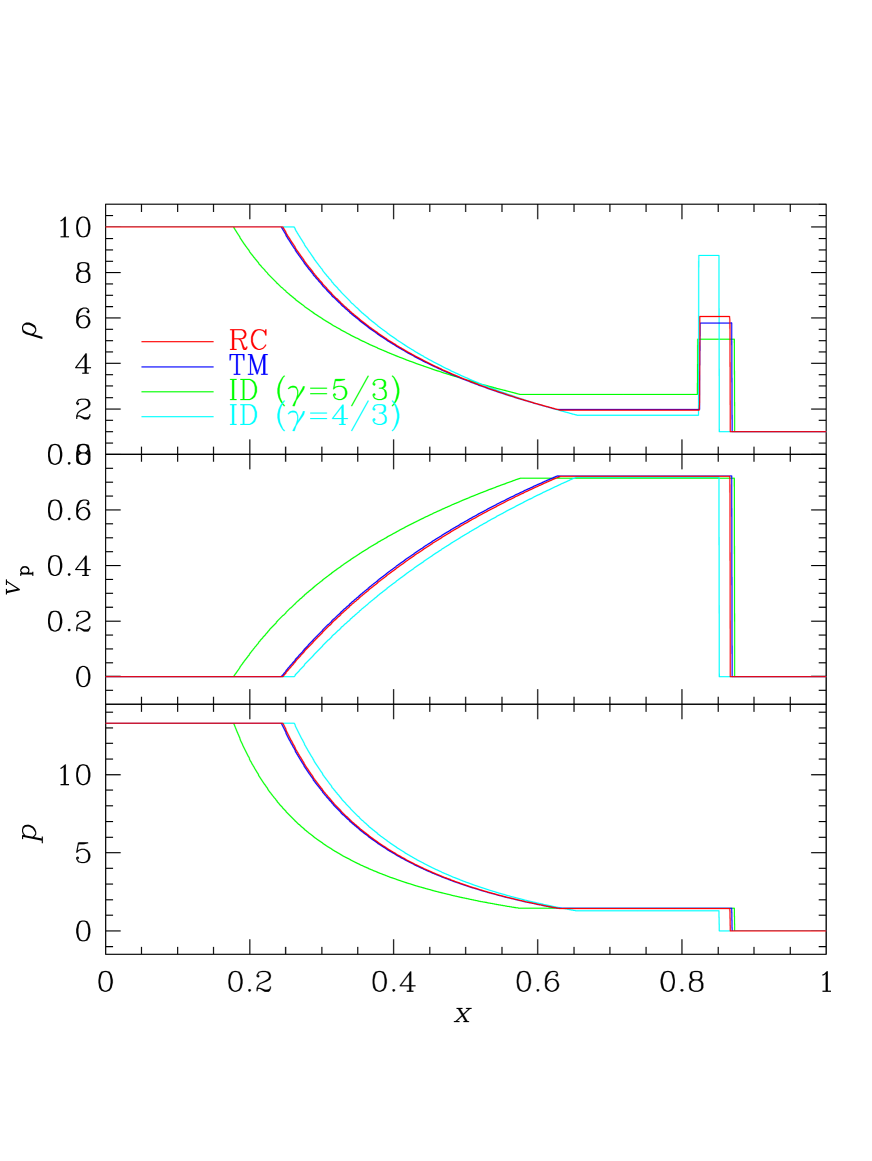
Figure 2: Relativistic shock tube with parallel component of velocity only (P1) with RC (red), TM (blue), and ID (green and cyan).

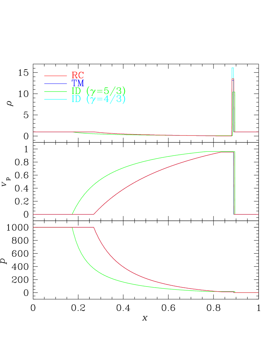
Figure 3: Relativistic shock tube with parallel component of velocity only (P2) with RC (red), TM (blue), and ID (green and cyan).

Figures 2 and 3 show the numerical solutions with RC and TM, and the analytic solutions with ID and $\gamma=5/3$ and $4/3$. The numerical solutions with RC and TM were obtained using the version of the TVD code having one velocity component (see section 4.1), and the analytic solutions with ID comes from the routine described in Martí & Müller (1994). The numerical solutions with ID are almost indistinguishable from the analytic solutions, once they are calculated.

The ID solutions with $\gamma=4/3$ and $5/3$ show noticeable differences. The density shell between the contact discontinuity (hereafter CD) and the shock becomes thinner and taller with smaller $\gamma$, because the post shock pressure is lower and so is the shock propagation speed. The rarefaction wave is less elongated with $\gamma=4/3$, because the sound speed is lower. Those solutions with ID are also clearly different from the solutions obtained with RC and TM. The ID solution with $\gamma=4/3$ better approximates the solutions with RC and TM in the left region of the CD, because the flow has relativistic temperature of $\Theta\gtrsim 1$ there. The difference is, however, obvious in the shell between the CD and the shock, because $\Theta\sim 1$ there. On the other hand, the solutions obtained with RC and TM look very much alike. It reflects the similarity in the distributions of specific enthalpy in equations (13) and (15). Yet there is a noticeable difference, especially in the shell between the CD and the shock, and the difference in density reaches up to $\sim 5\%$.

For the second set with transverse velocity component, four tests, where different transverse velocities were added to the test P2, are presented:
T1: initially $v_{t,R}=0.99$ to the right state, $t_{\rm end}=0.45$,
T2: initially $v_{t,L}=0.9$ to the left state, $t_{\rm end}=0.55$,
T3: initially $v_{t,L}=v_{t,R}=0.99$ to the left and right states, $t_{\rm end}=0.18$,
T4: initially $v_{t,L}=0.9$ and $v_{t,R}=0.99$ to the left and right states, $t_{\rm end}=0.75$.
The notations are the same ones used in P1 and P2. These are subsets of the tests originally suggested by Pons et al. (2000) with the ID EoS and later used by Mignone et al. (2005).

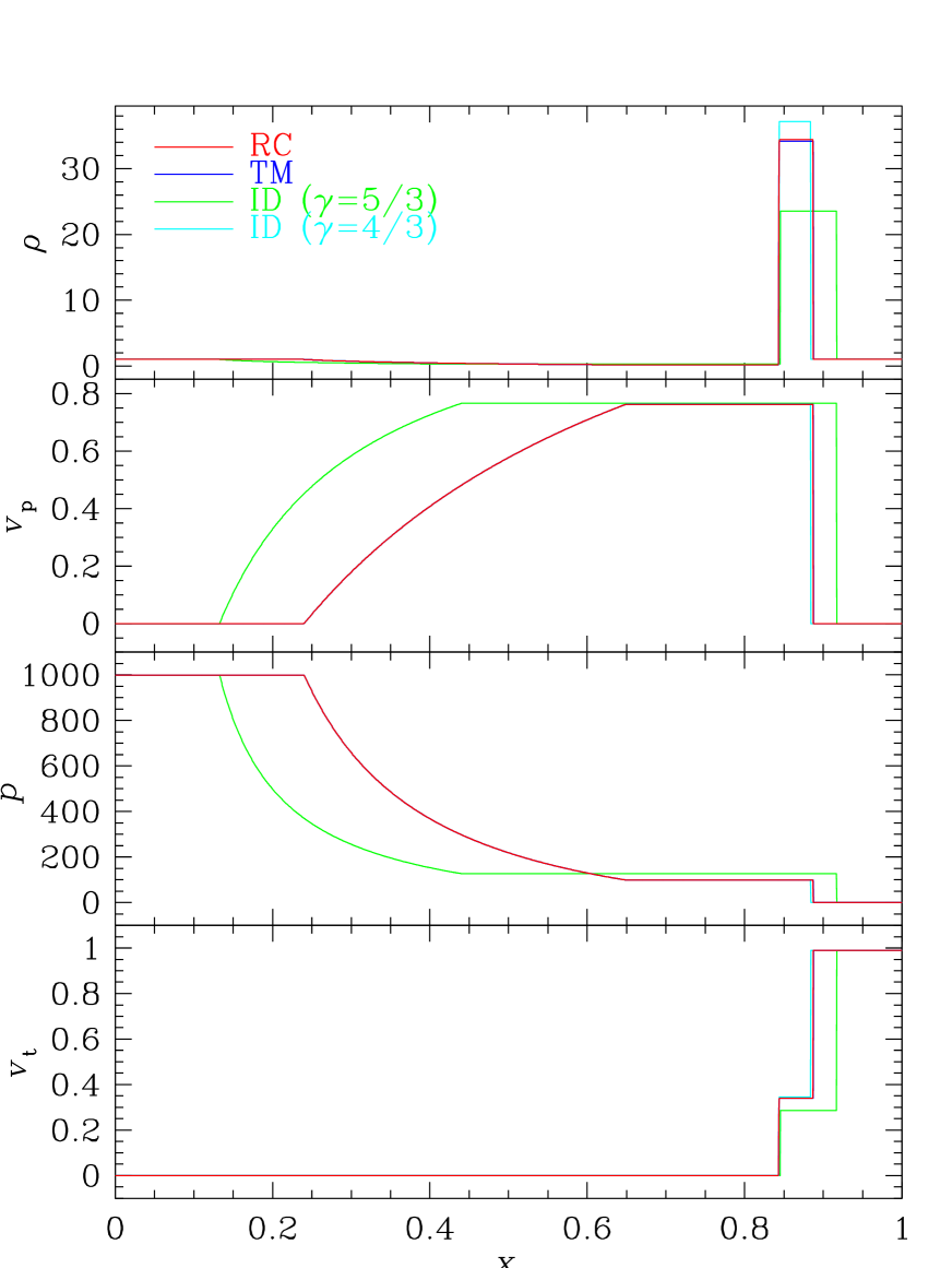
Figure 4: Relativistic shock tube with transverse component of velocity (T1) with RC (red), TM (blue), and ID (green and cyan).

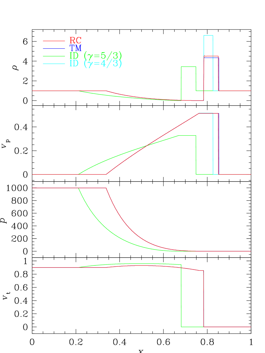
Figure 5: Relativistic shock tube with transverse component of velocity (T2) with RC (red), TM (blue), and ID (green and cyan).

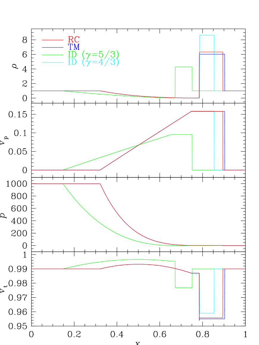
Figure 6: Relativistic shock tube with transverse component of velocity (T3) with RC (red), TM (blue), and ID (green and cyan).

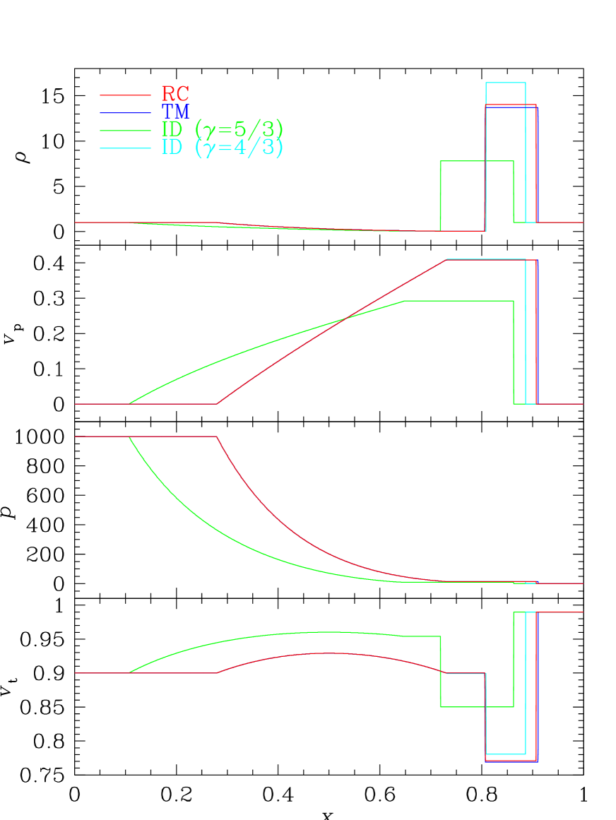
Figure 7: Relativistic shock tube with transverse component of velocity (T4) with RC (red), TM (blue), and ID (green and cyan).

Figures 4, 5, 6 and 7 show the numerical solutions with RC and TM and the analytic solutions with ID and $\gamma=5/3$ and $4/3$. The numerical solutions with RC and TM were obtained using the version of the TVD code having three velocity components (see section 4.2), and the analytic solutions with ID comes from the routine described in Pons et al. (2000).

Again the ID solutions with $\gamma=4/3$ and $5/3$ show noticeable differences. Especially with transverse velocity initially on the left side of the initial discontinuity (Figure 5, 6 and 7), the parallel velocity reaches lower values, while the transverse velocity achieves higher values, with higher $\gamma=5/3$ in the region to the left of the CD. As a result, the density shell between the CD and the shock has propagated less. As in the P tests, the solutions with ID are clearly different from the solutions obtained with RC and TM, most noticeably in the shell between the CD and the shock. The solutions with RC and TM look very much alike with differences in the density in the shell between the CD and the shock of about $\sim 5\%$.

We note that this paper is intended to focus on the EoS in numerical RHDs, not intended to present the performance of the code. Hence, one-dimensional tests of high resolution (with $2^{16}$ grid cells for the P tests and $2^{17}$ grid cells the T tests) are presented to manifest the difference induced by different EoS’s. The performance of the code such as capturing of shocks and CDs will be discussed elsewhere.

7 Summary and Discussion

The conservation equations for both Newtonian hydrodynamics and RHDs are strictly hyperbolic, rendering the apt use of upwind schemes for numerical codes. The actual implementation to RHDs is, however, complicated, partly due to EoS. In this paper we study three EoS’s for numerical RHDs, two being previously used and the other being newly proposed. The new EoS is simple and yet approximates the enthalpy of single-component perfect gas in relativistic regime with accuracy better than $0.8\%$. Then we discuss the calculation of primitive variables from conservative ones for the EoS’s considered. We also present the eigenvalues and eigenvectors of RHDs for a general EoS, in a way that they are ready to be used to build numerical codes based on the Roe-type schemes such as the TVD and ENO schemes. Finally we present numerical tests to show the differences in flow structure due to different EoS’s

The most commonly used, ideal EoS, can be used for the gas of entirely non-relativistic temperature ($\Theta\ll 1$) with $\gamma=5/3$ or for the gas of entirely ultrarelativistic temperature ($\Theta\gg 1$) with $\gamma=4/3$. However, if the transition from non-relativistic to relativistic or vice versa with $\Theta\sim 0.1-1$ is involved, the ideal EoS produces incorrect results and its use should be avoided. The EoS proposed by Mignone et al. (2005), TM, produces reasonably correct results with error of a few percent at most. The most preferable advantage of using TM is that the calculation of primitive variables admits analytic solutions, thereby making its implementation easy. The newly suggested EoS, RC, which approximates the EoS of the relativistic perfect gas, RP, most accurately, produces thermodynamically the most accurate results. At the same time it is simple enough to be implemented to numerical codes with minimum efforts and minimum computational costs. With RC the primitive variables should be calculated numerically by an iteration method such as the Newton-Raphson method. However, the equation for the calculation of primitive variables behaves extremely well, so the iteration converges in a few step without any trouble.

In Galactic and extragalactic jets and gamma-ray bursts, as the flows travel relativistic fluid speeds ($v\sim 1$ but $\Theta\ll 1$), they would hit the surrounding media. Then shocks are produced and the gas can be heated up to $\Theta\gtrsim 1$. These kind of transitions, continuous or discontinuous, between relativistic bulk speeds and relativistic temperatures are intrinsic in astrophysical relativistic flows, and so a correct EoS is required to simulate the flows correctly. The correctness as well as the simplicity make RC suitable for astrophysical applications like these.

Appendix A Jacobian Matrix with One Velocity Component

$$A=\frac{1}{N}\left(\begin{array}[]{ccc}A_{11}&A_{12}&A_{13}\\ A_{21}&A_{22}&A_{23}\\ 0&A_{32}&0\\ \end{array}\right)$$

$$A_{11}=v^{2}hn(1-c^{2}_{s})+\frac{vh}{\Gamma^{2}}$$

$$A_{12}=-\frac{1}{\Gamma^{3}}+\frac{1+n}{\Gamma}$$

$$A_{13}=-\frac{v(1+n)}{\Gamma}$$

$$A_{21}=-\frac{h^{2}}{\Gamma^{3}}(1-nc^{2}_{s})$$

$$A_{22}=-\frac{vh}{\Gamma^{2}}(1-nc^{2}_{s})+2vhn(1-c^{2}_{s})$$

$$A_{23}=-v^{2}hn(1-c^{2}_{s})+\frac{h}{\Gamma^{2}}$$

$$A_{32}=hn(1-c^{2}_{s}v^{2})$$

$$N=hn(1-c^{2}_{s}v^{2})$$

Appendix B Jacobian Matrix with Three Velocity Components

$$A_{x}=\frac{1}{N}\left(\begin{array}[]{ccccc}A_{11}&A_{12}&A_{13}&A_{14}&A_{15}\\ A_{21}&A_{22}&A_{23}&A_{24}&A_{25}\\ A_{31}&A_{32}&A_{33}&A_{34}&A_{35}\\ A_{41}&A_{42}&A_{43}&A_{44}&A_{45}\\ 0&A_{52}&0&0&0\\ \end{array}\right)$$

$$A_{11}=v_{x}hn(1-c^{2}_{s})+\frac{hv_{x}}{{\Gamma}^{2}}$$

$$A_{12}=\frac{1}{\Gamma}[n+v^{2}_{x}-nc^{2}_{s}(v^{2}_{y}+v^{2}_{z})]$$

$$A_{13}=\frac{1}{\Gamma}v_{x}v_{y}(1+nc^{2}_{s})$$

$$A_{14}=\frac{1}{\Gamma}v_{x}v_{z}(1+nc^{2}_{s})$$

$$A_{15}=-\frac{1}{\Gamma}v_{x}(1+n)$$

$$A_{21}=-\frac{1}{\Gamma}(1-v^{2}_{x})h^{2}(1-nc^{2}_{s})$$

$$A_{22}=v_{x}h[2n(1-c^{2}_{s}v^{2})-(1-v^{2}_{x})(1+nc^{2}_{s})]$$

$$A_{23}=-v_{y}h(1-v^{2}_{x})(1+nc^{2}_{s})$$

$$A_{24}=-v_{z}h(1-v^{2}_{x})(1+nc^{2}_{s})$$

$$A_{25}=-v^{2}_{x}h(1+n)+h(1+nc^{2}_{s}v^{2})$$

$$A_{31}=\frac{1}{\Gamma}v_{x}v_{y}h^{2}(1-nc^{2}_{s})$$

$$A_{32}=v_{y}h[n(1-c^{2}_{s}v^{2})+v^{2}_{x}(1+nc^{2}_{s})]$$

$$A_{33}=v_{x}h[n(1-c^{2}_{s}v^{2})+v^{2}_{y}(1+nc^{2}_{s})]$$

$$A_{34}=v_{x}v_{y}v_{z}h(1+nc^{2}_{s})$$

$$A_{35}=-v_{x}v_{y}h(1+n)$$

$$A_{41}=\frac{1}{\Gamma}v_{x}v_{z}h^{2}(1-nc^{2}_{s})$$

$$A_{42}=v_{z}h[n(1-c^{2}_{s}v^{2})+v^{2}_{x}(1+nc^{2}_{s})]$$

$$A_{43}=v_{x}v_{y}v_{z}h(1+nc^{2}_{s})$$

$$A_{44}=v_{x}h[n(1-c^{2}_{s}v^{2})+v^{2}_{z}(1+nc^{2}_{s})]$$

$$A_{45}=-v_{x}v_{z}h(1+n)$$

$$A_{52}=hn(1-c^{2}_{s}v^{2})$$

$$N=hn(1-c^{2}_{s}v^{2})$$

References

- Abramowitz & Stegun (1972) Abramowitz, M. A. & Stegun, I. A. 1972, Handbook of Mathematical Functions (Dover: Dover Publishing Company)
- Aloy et al. (1999) Aloy, M. A., Ibáñez, J. M., Martí, J. M. & Müller, E. 1999, ApJS, 122, 151
- Choi & Ryu (2005) Choi, E. & Ryu, D., 2005, New Astronomy, 11, 116
- DelZanna & Bucciantini (2002) DelZanna, L. & Bucciantini, N. 2002, A&A, 390, 1177
- Donat et al. (1998) Donat, R., Font, J. A., Ibáñez, J. M. & Marquina, A. 1998, J. Comput. Phys., 146, 58
- Dolezal & Wong (1995) Dolezal, A. & Wong, S. S. M. 1995, J. Comput. Phys., 120, 266
- Eulderink & Mellema (1995) Eulderink, F. & Mellema, G. 1995, A&A, 110, 587
- Falle & Komissarov (1996) Falle, S. A. E. G & Komissarov, S. S., 1996, MNRAS, 278, 586
- Harten (1983) Harten, A. 1983, J. Comput. Phys., 49, 357
- Landau & Lifshitz (1959) Landau, L. D. & Lifshitz, E. M. 1959, Fluid Mechanics (New York: Pergamon Press)
- Martí & Müller (1994) Martí, J. M. & Müller, E. 1994, J. Fluid Mech., 258, 317
- Martí & Müller (1996) Martí, J. M. & Müller, E. 1996, J. Comput. Phys., 123, 1
- Martí & Müller (2003) Martí, J. M. & Müller, E. 2003, Living Rev. Relativity, 6, 7
- Mathews (1971) Mathews, W. G. 1971, ApJ, 165, 147
- Mészáros (2002) Mészáros, P. 2002, ARA&A, 40, 137
- Mignone et al. (2005) Mignone, A., Plewa, T. & Bodo, G. 2005, ApJS, 160, 199
- Mignone & Bodo (2005) Mignone, A. & Bodo, G. 2005, MNRAS, 364, 126
- Mirabel & Rodríguez (1999) Mirabel, I. F., & Rodríguez, L. F. 1999, ARA&A, 37, 409
- Pons et al. (2000) Pons, J. A., Martí, J. M. & Müller, E. 2000, J. Fluid Mech., 422, 125
- Roe (1981) Roe, P. L. 1981, J. Comput. Phys., 43, 357
- Ryu et al. (1993) Ryu, D., Ostriker, J. P., Kang, H. & Cen, R. 1993, ApJ, 414, 1
- Rahman & Moore (2005) Rahman, T. & Moore, R. 2005, preprint (astro-ph/0512246)
- Schneider et al. (1993) Schneider, V., Katscher, U., Rischke, D. H., Waldhauser, B., Maruhn, J. A. & Munz, C.-D. 1993, J. Comput. Phys., 105, 92
- Sokolov et al. (2001) Sokolov, I., Zhang,H. M.& Sakai, J. I. 2001, J. Comput. Phys., 172, 209
- Synge (1957) Synge, J. L. 1957, The Relativistic Gas (Amsterdam: North-Holland Publishing Company)
- Taub (1948) Taub, A. H. 1948, Phys. Rev., 74, 328
- Wilson & Mathews (2003) Wilson, J. R. & Mathews, G. J. 2003, Relativistic Numerical Hydrodynamics (Cambridge: Cambridge Univ. Press)
- Zensus (1997) Zensus, J. A. 1997, ARA&A, 35, 607