New Chandra observations of the jet in 3C 273.
I. Softer X-ray than radio spectra and the X-ray emission mechanism

Abstract

The jet in 3C 273 is a high-power quasar jet with radio, optical and X-ray emission whose size and brightness allow a detailed study of the emission processes acting in it. We present deep Chandra observations of this jet and analyse the spectral properties of the jet emission from radio through X-rays. We find that the X-ray spectra are significantly softer than the radio spectra in all regions of the bright part of the jet except for the first bright “knot A”, ruling out a model in which the X-ray emission from the entire jet arises from beamed inverse-Compton scattering of cosmic microwave background photons in a single-zone jet flow. Within two-zone jet models, we find that a synchrotron origin for the jet’s X-rays requires fewer additional assumptions than an inverse-Compton model, especially if velocity shear leads to efficient particle acceleration in jet flows.

1. Introduction

Since the launch of the Chandra X-ray observatory, it has become evident that X-ray emission is a common feature of jets in radio galaxies and quasars (see, e.g., Worrall et al. 2001 for low-power radio galaxies, Sambruna et al. 2004 and Marshall et al. 2005b for X-ray surveys of powerful radio galaxies and quasars, the overview articles by Harris & Krawczynski 2002 and Kataoka & Stawarz 2005 for emission mechanisms, and the XJET home page for an up-to-date list of X-ray emission associated with extragalactic jets). Typically, the X-ray emission from low-power jets (Fanaroff & Riley, 1974 [FR] class I) fits on a single synchrotron spectrum with their radio and optical emission and is thus satisfactorily explained as synchrotron emission (with the interesting problem of having to accelerate X-ray emitting synchrotron electrons in situ). However, the spectral energy distribution (SED) of high-power (FR II) jets usually shows the so-called “bow-tie” problem, i.e., their X-ray spectrum does not fit on an extrapolation of the observed radio/optical synchrotron spectrum. A representative case in point is the first new X-ray jet detection by Chandra, PKS 0637-752 (Schwartz et al., 2000; Chartas et al., 2000), with an observed cutoff to the synchrotron emission in the optical range, but a fairly hard X-ray spectrum ($\alpha\approx-0.7$) and an X-ray flux per frequency decade (i.e., $\nu S_{\nu}$) exceeding the optical one. As the predicted X-ray intensity from synchrotron self-Compton (SSC) emission is usually orders of magnitude below the observed one, it has been suggested that these jets are still highly relativistic at kiloparsec scales, with bulk Lorentz factors in the range 5–30 and beyond, and that the X-rays are inverse-Compton (IC) scattered cosmic microwave background (CMB) photons (the beamed IC-CMB process; Tavecchio et al., 2000; Celotti et al., 2001). The high Lorentz factors are necessary in order for the energy density of the CMB photon field to be boosted sufficiently in the jet rest frame (by a factor $\Gamma^{2}$, where $\Gamma$ is the bulk Lorentz factor of the jet fluid) to account for the observed X-ray:radio flux ratios.

The beamed IC-CMB process is generally invoked to account for the X-ray emission from jets in which a single synchrotron component cannot account for the emission in all wavebands. If correct, the inferred values of $\Gamma$ would constitute the first firm measurement of the velocity of high-power jets (for the velocities of low-power jets, see the modeling by Laing & Bridle, 2004; Canvin & Laing, 2004; Canvin et al., 2005) with profound implications for the analysis of jet energetics and composition. Since the increase of the CMB energy density with redshift would cancel the surface brightness dimming with redshift, beamed IC-CMB X-ray jets at high redshift could be cosmic beacons that outshine their quasars (Schwartz, 2002). Moreover, there are jets in FR II radio galaxies and quasars whose X-ray emission is either well explained as synchrotron emission on an extrapolation of the radio-optical spectrum (e.g., in some of the jets in the survey by Sambruna et al. 2004, and that in 3C 403 [Kraft et al., 2005]), or because the necessary Doppler factors cannot be achieved from geometrical considerations, such as in Pictor A (Hardcastle & Croston, 2005) where there is X-ray emission from the counter-jet as well as the approaching jet. A detailed check of the beamed IC-CMB model is therefore warranted.

There are two basic testable predictions of the beamed IC-CMB model which arise from the fact that those electrons responsible for the upscattering of CMB photons into the X-ray band have low Lorentz factors ($10\lesssim\gamma\lesssim 100$) and hence emit synchrotron radiation at wavelengths of a few tens or hundreds of Megahertz, below the typical Gigahertz-range observing frequencies allowing high-resolution studies of radio jets. Essentially, a similar part of the electron energy distribution can be observed in two different wavebands (the electrons producing IC emission in the Chandra band emit synchrotron radiation in the range 40 Hz–1 MHz; Harris & Krawczynski, 2002), leading us to expect a close correspondence both of morphology and of spectral index between a beamed IC-CMB jet’s X-ray and radio emission.

We have chosen the jet in 3C 273 for a detailed test of the beamed IC-CMB model with the Chandra X-ray Observatory. This jet has a unique combination of properties that make it worthy of detailed study: it has a large angular size (bright radio, optical and X-ray emission being observed from 11″ out to 22″ from the core), it is one of the closest high-power jets ($z=0.158$) so that smaller physical scales can be resolved than in most similar jets, and high-resolution VLA and HST data are available (Jester et al., 2005, and references therein) that allow the construction of detailed SEDs and the study of the relation between the jet’s X-rays and the radio-optical synchrotron emission. 3C 273’s jet is among those from which X-ray emission had been detected already with the Einstein satellite (Willingale, 1981; Harris & Stern, 1987). Based on a comparison of ROSAT HRI observations with radio and optical data, Röser et al. (2000) concluded that the X-ray emission could only be due to the same synchrotron component as the jet’s radio-optical emission in the first bright feature of the jet (“knot A”), but not in the remainder of the jet, where there is a cutoff to the synchrotron component in the near-infrared/optical range; later, Jester et al. (2002) and Jester et al. (2005) showed that at 0$\farcs$3 resolution, already the radio-optical SEDs of most of the jet, including knot A, require a two-component model to account for the emission. Hence, the X-ray emission there cannot be due to a single radio–optical–X-ray synchrotron component, either (but see Fleishman, 2006, who suggests that an additional contribution of synchrotron emission from particles moving in fields that are tangled on small scales may explain the observed flattening, at least in parts of the jet). Jester et al. (2002) suggested that the second optical component may be the same component as the jet’s X-ray emission, but could not constrain the emission mechanism for the high-energy component further.

Regarding the X-ray emission mechanism, Röser et al. (2000) ruled out SSC as well as thermal Bremsstrahlung. The first Chandra observations of this jet were presented by Sambruna et al. (2001) and Marshall et al. (2001). Marshall et al. (2001) presented the first X-ray image of this jet with both high resolution and high signal-to-noise ratio. Regarding the SEDs, they came to similar conclusions as Röser et al. (2000). Sambruna et al. (2001) had analyzed a smaller set of the early Chandra data and favored a beamed IC-CMB model for the emission from all parts of the jet. Marshall et al. (2001) compared the optical and X-ray morphology at the Chandra resolution of 0$\farcs$78 and found that the X-ray and optical emission come from the same parts of the jet and show very similar features. However, there are offsets between the X-ray and optical peaks in one or both of the first two bright knots. In the remainder of the jet, the relative variations in X-ray brightness are smaller than those in the radio and optical. Such size and brightness differences require some parameter fine-tuning in the IC-CMB model.

Thus, previous observations had left the nature of the X-ray emission mechanism of 3C 273 unclear. Here, we present a spectral analysis of our new Chandra observations, which we combine with archival data and our VLA + HST dataset from Jester et al. (2005). Observations and data reduction are described in §2, our spectral analysis and its results are presented in §3, and we discuss in §4 the implications of our results for the beamed IC-CMB model and other emission mechanisms. We summarize our findings in §5.

2. Observations and data reduction

We have obtained four observations of 3C 273 and its jet in Chandra observing cycle 5, totaling just under 160 ksec observing time. The observations were split into four exposures of equal length in order to search for variability within the observing cycle. The quasar and jet were placed on the ACIS-S3 chip in each of these. We also use calibration observations of 3C 273 from the Chandra archive: two ACIS-S3 data sets from cycle 1, with 30 ksec exposure time each, and seven ACIS+HETG calibration observations, totaling just under 200 ksec. The gratings only transmit about 10% of the soft X-ray photons ($E<2$ keV), but about 75% of the hard X-ray photons ($E>6$ keV). Hence, we use the grating data to perform consistency checks on the spectral shape of the jet at the high-energy end of the Chandra bandpass. We will not use them for morphological analysis. This decision is based purely on the fact that their inclusion would have required substantial additional effort without a commensurate gain in the total number of detected photons; as the calibration data were used by the calibration team to check the effective area, not the pileup or contamination correction, they could be used without causing any circular reasoning. Table 1 gives the observing log.

Table 1Observing log for ACIS observations of 3C 273.

Grating	ObsId	Exp. time	Obs. start time	Frame time
		ksec	UT	sec
None	1711	28.09	2000-06-14 05:13:19	1.1
	1712	27.80	2000-06-14 13:43:27	3.2
	4876	41.30	2003-11-24 23:08:40	0.4
	4877	38.44	2004-02-10 03:40:39	0.4
	4878	37.59	2004-04-26 20:55:16	0.4
	4879	39.23	2004-07-28 03:35:33	0.4
HETG	459	39.06	2000-01-10 06:46:11	2.5
	2463	27.13	2001-06-13 06:41:21	2.1
	3456	25.00	2002-06-05 10:03:12	1.9
	3457	25.38	2002-06-05 17:19:11	2.5
	3573	30.16	2002-06-06 00:43:51	2.5
	4430	27.60	2003-07-07 12:08:58	3.2
	5169	30.17	2004-06-30 12:39:18	2.5

Note. — All grating-free observations used the ACIS-S3 chip. ObsIds 1711 and 1712 and all HETG observations are from calibration programs, ObsIds 4876-4879 were obtained under Chandra GO proposal 05700741.

We used the Chandra analysis software CIAO v. 3.2 or later and calibration database CALDB v. 3.0 or later to reprocess all data, taking advantage of updated calibrations, in particular the ACIS contamination correction (Marshall et al., 2004), and to remove the pixel randomization. The spectral analysis (see following section) was performed using spectral fits in the Sherpa software package (Freeman et al., 2001). In addition, we constructed flux-calibrated brightness maps for the ACIS-S3 observations.

Registering Chandra data sets is challenging. The absolute pointing calibration of Chandra of about 0$\farcs$4 (Chandra X-ray Center, 2005a, Table 5.1) is not sufficient for our analysis, since the jet width is only about 1″. The quasar core is the only bright X-ray point source in the vicinity of the jet, but it is so bright that it is severely piled up (Chandra X-ray Center, 2005a, Section 6.14) even with a frame time of 0.4 s (chosen in our new observations) or with the HETG in place. However, the readout streak in the grating-free observations contains so many counts that it can be used to constrain the location of the quasar core in the perpendicular direction with high precision and accuracy. The unpiled wings of the PSF provide the necessary second constraint. We further attempt to mitigate the effect of pileup by constructing an “eV per second” (evps) map, an energy-weighted count rate map. Three of the authors (SJ, DEH, HLM) have performed independent fits of the non-piled up part of the PSF and the readout streak, both on the evps maps and on the brightness maps, to obtain the position of the quasar core in each of the six ACIS-S3 sets. From the RMS of the individual determinations, we estimate that the alignment is better than 0$\farcs$1 in each coordinate. We average the individual measurements to get a final quasar position in “physical” ACIS coordinates. We then update the world coordinate system (WCS) of the individual event files and maps to assign 3C273’s right ascension and declination as determined from radio observations to the quasar’s fitted physical coordinates. For the HETG zeroth-order images, which are used for consistency checks, we fit a Gaussian to the wings of the quasar image to fix the astrometry relative to the quasar core.

3. Analysis and results

3.1. Source extraction regions, variability search, and spectral fits

3.1.1 Extraction regions

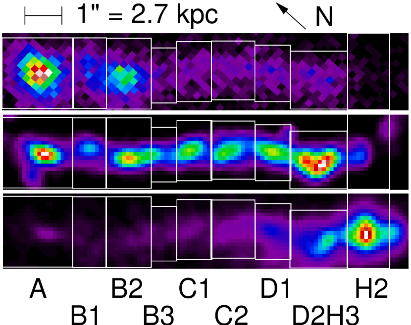
Figure 1.— The jet in 3C273 observed with Chandra (top), HST ($\lambda=620$ nm, middle) and VLA ($\lambda=$3.6 cm, below). The long edges of each image are along a position angle of 222°; the physical size of the region covered by each image is 5.7 kpc by 28.6 kpc. The boxes indicate the regions adopted for the analysis in this paper. The VLA and HST map and the labeling scheme are taken from Jester et al. (2005), with a resolution of 0$\farcs$3 (810 pc) and a pixel size of 0$\farcs$1 (270 pc). The Chandra map is from ObsId 4876, with counts binned in 0$\farcs$166 (450 pc) pixels and a resolution of 0$\farcs$78 FWHM (2.1 kpc).

We perform a separate spectral analysis in each of nine regions, which we have defined considering both the radio/optical and X-ray morphology. Figure 1 shows the regions on a Chandra, HST and VLA image. The nomenclature for the subdivisions of the original regions ABCD (Lelievre et al., 1984) is that established by Röser & Meisenheimer (1991, their Table 4); later, Bahcall et al. (1995) and thence Marshall et al. (2001) used different subdivisions. There are no gaps between the extraction regions, and each is about 1-2″ in size.

While the jet shows similar morphology at all wavelengths, there are differences in some places, which create some ambiguity as to where the boundaries between different jet regions (or knots) should be placed. The differences in morphology at different wavelengths imply spatial variations in the spectral shape. Hence, some of our measurement regions mix emission from jet features with different spectral shapes. Given that the Chandra resolution of 0$\farcs$78 (full-width at half-maximum intensity of a Gaussian fitted to the readout streak) is comparable to the typical diameter of the jet features, such mixing of spectral shapes cannot be avoided entirely. However, the morphology differences are mostly minor, the sole exception being region B1, in which the X-ray and optical emission clearly arch to the north, while the radio emission has an arc to the south (compare Marshall et al., 2001). This difference may in fact contain a crucial hint to the nature of the emission and particle acceleration mechanism acting in the jet; however, the two arcs are not fully resolved by Chandra, so that we include both in a single region. Still, the need to consider the emission from the arcs in B1 separately should be borne in mind when analyzing the spectral shape there.

For the estimation of the background count rate, we define annuli of similar radial extent as the corresponding jet region that are centered on the quasar, as large-angle scattered photons from the quasar core are the dominant contribution to the background. The background regions exclude the jet regions themselves as well as the readout streak.

Considering the locations of those events classified as “afterglow events” by the CIAO pipeline suggests that ObsIds 1711 and 1712 include some piled-up events at the brightness peak of region A. The other ACIS-S3 observations used a 1/8th subarray, shortening the frame time correspondingly, and therefore do not suffer from pileup. The HETG observations have lower count rates in the jet and pileup is much less than 1% there.

To determine the flux and X-ray spectral index, we extract spectra and response files for each source region using the psextract CIAO script.

3.1.2 Variability search

We searched for variability in the count rates of each of the regions over all six ACIS-S3 data sets and found no variations in excess of the expected Poisson fluctuations for a constant count rate. In addition, we performed separate Sherpa power-law fits for each knot and each epoch, as detailed below. We used the $\chi^{2}$ test to assess the significance of the fluctations. The observed fluctuations and their probabilites are given in Table 2. In nearly all regions, the $\chi^{2}$ test returned very high probabilities for obtaining the observed fluctuations in the fit parameters across the six epochs as random fluctuations of an underlying spectrum with both constant flux and spectral index. Only the flux variability for region D2H3 is significant at the 96% confidence level; however, at 3%, it is also amongst the smallest observed fluctuations, and there is no systematic trend. Thus, there is no detection of significant systematic variability in any of the regions.

Table 2Results of variability search

Region	Flux RMS	$p$	Spectral RMS	$p$
	%		%
A	6	0.92	4	0.90
B1	9	0.99	8	0.88
B2	7	1.00	2	0.08
B3	5	0.08	11	0.49
C1	6	0.35	9	0.58
C2	4	0.10	7	0.40
D1	9	0.75	9	0.51
D2H3	3	0.04	6	0.39
H2	14	0.12	18	0.16

Note. — Variability of jet features fitted with a power-law model as in § 3.1.3

In the remainder of this paper, we therefore concentrate on the question whether the spectral shape of the jet emission is consistent with the beamed inverse-Compton model. The morphology will be discussed in detail in a separate paper.

3.1.3 Spectral fits

For the analysis in the remainder of the paper, we combine all six epochs of ACIS-S data. In each region, we perform a joint Sherpa spectral fit for data and background, using simple power laws to describe both the source and the background components. As the quasar itself shows both spectral and flux variability in the soft X-ray band (McHardy et al., 1999), we allow an independent background model component for every epoch. We include a JDPileup model (Davis, 2001) for the fit of region A in ObsIDs 1711 and 1712; the use of this model is appropriate since this region is unresolved by Chandra (Marshall et al., 2001, 2005a) and it is justified by the fit results which indicate a pileup fraction of 3.6% and 9.4%, respectively. Trial fits including a pileup model for the other 4 data sets and for all other jet regions had results consistent with 0 piled up events, even though scaling the piled up fraction by the frame time would lead us to expect a pileup fraction of about 1% (see frame times in Table 1). As in Marshall et al. (2001), we use the hydrogen column density of $n_{\mathrm{H}}=1.71\times 10^{20}$ cm^-2 given by Albert et al. (1993). We perform fits using two methods. First, we used the likelihood method (Cash statistic; Chandra X-ray Center, 2005b) for unbinned events, using only the energy range 0.5 keV–8.0 keV. Secondly, we grouped the data to a minimum of 15 counts per bin with $\chi^{2}$ Primini statistics (Chandra X-ray Center, 2005b), in this case excluding all bins below 0.5 keV. We do separate fits for the data from the HETG zeroth-order images and from the grating-free observations. The fit results from both data sets (HETG zeroth-order images and grating-free S3 images) and both fitting methods (unbinned/Cash and grouped/$\chi^{2}$) are consistent with each other. We have carried out further spot checks using XSPEC power-law fits of the grouped data sets, in which background events are subtracted before fitting (instead of being included in the fit as a separate model component), and found excellent agreement with the Sherpa results. Thus, the following analysis will make use of the fit parameters obtained from the fits of unbinned data with Cash statistics, and in the remainder of the paper, we only bin data for display purposes.

3.2. Fit results and SEDs from radio to X-rays

Table 3Fit results for joint X-ray spectral fits

Region	Net counts	$\alpha$	$\sigma_{\alpha}$	$S_{\nu}(1\,\mathrm{keV})$	$\sigma_{S}$
				nJy	nJy
A	10849	$-$0.83	0.02	46.54	0.54
B1	2632	$-$0.80	0.03	10.89	0.25
B2	3992	$-$0.97	0.03	19.98	0.33
B3	768	$-$1.13	0.07	3.41	0.14
C1	1115	$-$1.07	0.06	4.85	0.16
C2	1467	$-$0.96	0.05	6.25	0.18
D1	1182	$-$1.02	0.05	5.16	0.17
D2H3	1707	$-$1.04	0.04	7.82	0.20
H2	317	$-$1.27	0.12	1.30	0.09

Note. — The fits were done on the six ACIS-S3 data sets without grating, using original events in the range 0.5 keV–8.0 keV with Cash statistics in Sherpa. Spectral indices are defined such that $S_{\nu}\propto\nu^{\alpha}$.

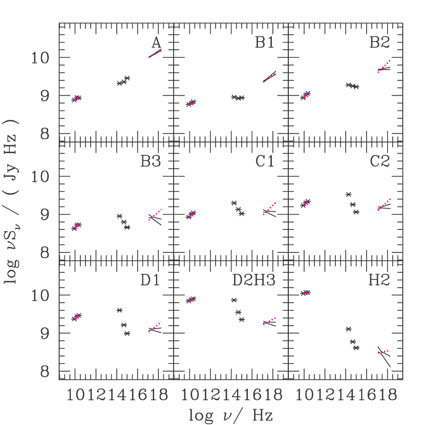
Figure 2.— Spectral energy distributions for the jet regions defined in Fig. 1. The radio and optical points are obtained by integrating the flux from the maps at 0$\farcs$3 resolution from Jester et al. (2005) over the same extraction regions as the X-rays. Error bars for radio and optical data show random errors; there may be additional calibration and flat-fielding errors of up to 3% for the near-infrared and optical data points. The magenta solid line in the radio region is a least-squares power-law fit to the three VLA data points; the dotted line in the X-ray band has the same spectral index as the VLA data and the same flux density at 1 keV as the Chandra data, to allow a comparison of X-ray and radio spectral indices.

Figure 3.— Comparison of radio and X-ray spectral indices for the jet regions from Fig. 1. The X-ray spectral index and its error are obtained from the Sherpa fit. The radio spectral index is the same least-squares fit shown in Fig. 2, its error has been calculated from the signal-to-noise ratio of the VLA maps. The dotted line shows equality of both spectral indices. Except for regions A and B1, the X-ray spectrum is significantly softer than the radio spectrum.

Table 3 gives the fit results. In all cases, a simple power law was a good fit to the data, according to the probabilities obtained for the $\chi^{2}$ fits. We also generated X-ray SEDs in six energy bands from corresponding brightness maps. The SEDs for knots A and B2 show some curvature in the range 4–5keV and a slightly softer spectrum at lower energies than the Sherpa fits, which would be consistent with a marginally detected high-energy cutoff. However, no evidence for a cutoff was found in the fits using the event lists, neither in the pure power-law fits nor in fits with a cut-off power law (Sherpa model xscutoffpl). The X-ray spectral indices of A and B1 are consistent with each other and both approximately $-0.8$. The knots in the remainder of the jet have slightly softer X-ray spectra; all knots from B2 up to and including D2H3 again have spectral indices that are consistent with each other and a value of $-1.010\pm 0.018$.

The radio hot spot region H2 is significantly detected in X-rays in the combined data set; in fact, Marshall et al. (2001) already noted that the jet was detected out to 22″ from the core, with the radio peak in H2 being located 21$\farcs$4 from the core. A comparison of the X-ray flux profile of regions D2H3 and H2 with that of the nearly point-like region A confirms the reality of the detection of H2. Its spectrum is marginally softer than the rest of the jet.

Figure 2 shows the spectral energy distributions (SEDs) of the nine jet regions from radio up to X-rays. It is evident from the SEDs that the jet emission from radio up to X-rays cannot be explained as a single synchrotron component for any part of the jet. Except for region A, this was already known from the analysis of ROSAT data (Röser et al., 2000) and of the first Chandra data sets (Marshall et al., 2001; Sambruna et al., 2001). Jester et al. (2002, 2005) showed that a single-component synchrotron spectrum was not in fact viable for knot A, chiefly because the new multi-frequency multi-configuration VLA data set used by them, and here, yielded substantially different radio SED shapes.

Our spectral index measurement for knot A of $\alpha=-0.83\pm 0.02$ is consistent with the 90% confidence interval $\alpha_{x}=1.1^{+0.5}_{-0.3}$ given by Sambruna et al. (2001) at the $1.5\,\sigma$ level. However, Marshall et al. (2001) obtained a much harder X-ray spectrum with $\alpha=-0.60\pm 0.05$. The discrepancy is due to two systematic effects. First, pileup slightly hardened the data used by Marshall et al.. Secondly, corrections for ACIS contamination, which absorbs X-ray photons mostly below 1 keV, were released only after publication of their paper (see Marshall et al., 2004). We can reproduce the Marshall et al. result by turning off the pileup and contamination correction.

In Fig. 3, we compare the radio and X-ray spectral indices directly. It clearly shows the basic and important finding of our spectral analysis: except for regions A and B1, the X-ray spectrum is significantly softer than the radio spectrum.

4. Discussion: Implications of the new SEDs for the X-ray emission mechanism

The aim of the Chandra observations presented here was a test of both the synchrotron and the beamed IC-CMB models for the jet’s X-ray emission. The non-detection of significant variability does not rule out synchrotron as X-ray emission process, as the Chandra resolution element is sufficiently large (the FWHM of 0$\farcs$78 corresponds to 2.1 kpc) to allow possible variability to be washed out. We now discuss the implications of the observed SED shape for both synchrotron and beamed IC-CMB as X-ray emission mechanism. The models have to account for the following observational facts:

1. There is a spectral hardening of the near-infrared/optical/ultraviolet emission in all parts of the jet see the SEDs in Jester et al., 2002 and Fig. 2, but in particular those in Jester et al., 2005. The shape of the second optical/UV emission component cannot be constrained to a high degree of certainty based on the present data set, but it may well be the extrapolation of the X-ray power law to lower frequencies (Jester et al., 2002).

2. The X-ray emission cannot be explained by a simple extrapolation of the total optical emission (the “bow-tie” problem; see Röser et al., 2000; Sambruna et al., 2001; Marshall et al., 2001).

3. The radio synchrotron emission from the jet in 3C 273 has a spectral index $\alpha\approx-0.75$ at all observed frequencies, down to 330 MHz Conway et al., 1993 and confirmed by our unpublished VLA data.

4. Radio and optical emission show very similar degrees of linear polarization out to 18″ from the core, and the polarization vectors are parallel to each other in all parts of the jet except for the optically quiet radio “backflow” or “cocoon” to the south of the jet (Röser & Meisenheimer, 1991; Röser et al., 1996).

5. The X-ray emission has a softer spectrum than the radio emission in most parts of the jet (Figures 2 and 3).

6. The same morphological features are seen at all wavelengths, from radio to optical (Bahcall et al., 1995) to X-rays (Sambruna et al., 2001; Marshall et al., 2001).

Items 1 and 2 individually rule out a one-zone synchrotron model, but would be compatible with a two-zone synchrotron model as well as an IC-CMB model with one or more zones. Item 3 implies that the jet’s total radio emission is dominated by a single synchrotron component down to the lowest currently observed frequencies. The high linear polarization (item 4) lead to the conclusion that the optical emission is synchrotron light (Röser & Meisenheimer, 1991), and the similarity of the radio and optical polarization indicated that the radio and optical synchrotron emission are due to the same electron population (Röser et al., 1996). Remarkably, if the X-ray emission could be shown to be of the same origin as most, and not just some, of the optical emission (compare Jester et al., 2002), the fact that the optical emission is synchrotron would imply that the X-ray emission is synchrotron, too; this might be expected from the similarity of the optical and X-ray morphology (item 6 above), and is very strongly supported by the analysis of Spitzer mid-infrared observations by Uchiyama et al. (2006). The clarification of this issue requires the analysis of further mid-infrared (Spitzer) and ultraviolet (HST) data. For now, we discuss the viability of the IC-CMB and the two-zone synchrotron models given item 5.

4.1. Viability of the IC-CMB model

4.1.1 Single-zone IC-CMB

In the beamed IC-CMB model, CMB photons are upscattered into the Chandra band by electrons with Lorentz factors of order 50-200 in a jet with bulk Lorentz factor $\Gamma$ and Doppler factor $\delta$, photons with incoming energy $E_{\mathrm{cmb}}$ are upscattered to energy $E_{\mathrm{x}}$ by electrons with Lorentz factor $\gamma\approx(E_{\mathrm{x}}/E_{\mathrm{cmb}}/[\Gamma\,\delta\,(1+z)])^{1/2}$, and we used $\Gamma=\delta=15$, z = 0.158, $0.5\,\mathrm{keV}<E_{\mathrm{x}}<8\,\mathrm{keV}$, $E_{\mathrm{cmb}}=6.6\times 10^{-4}$ eV; see Harris & Krawczynski, 2002. Using the formula for the characteristic frequency $\nu_{\mathrm{c}}$ of synchrotron emission for electrons with Lorentz factor $\gamma$ in a magnetic field with flux density $B$, $\nu_{\mathrm{c}}=4.2\,\mathrm{MHz}\;B/(10\,\mathrm{nT})\,(\gamma/100)^{2}\,\delta\,/(1+z)$ ($10\,\mathrm{nT}\mathrel{\widehat{=}}100\,\mu$G), we obtain that these same electrons produce synchrotron emission at frequencies 20–250 MHz $\times B/(10\,\mathrm{nT})$ i.e., at lower frequencies than the VLA observations presented here (the minimum-energy field in this jet is of order 10–20 nT for $\delta=1$, and an order of magnitude smaller for $\delta=15$; Jester et al., 2005; Harris & Krawczynski, 2002; Stawarz et al., 2003). The electron energy distribution should be either a power law, or have curvature such that lower-frequency emission has a harder spectrum. Hence, in the beamed IC-CMB model one expects that the X-ray spectrum should have a spectrum that has the same spectral index as, or is harder than, the radio emission from the jet.

As shown by Figures 2 and 3, the X-ray spectrum is significantly softer than the radio spectrum in all parts of the jet except for regions A and B1. When the beamed IC-CMB model is put forward to account for X-ray emission from high-power radio jets, or used to infer physical parameters such as the Doppler factor and the line-of-sight angle, the usual assumption is a single-zone single-component model, i.e., one in which the electron population producing synchrotron emission is identical to that upscattering CMB photons into the X-ray band (see Tavecchio et al., 2000; Sambruna et al., 2001; Harris & Krawczynski, 2002; Sambruna et al., 2004; Kataoka & Stawarz, 2005; Marshall et al., 2005b, e.g.) and where identical jet volumes contribute to the synchrotron and inverse-Compton emission. This conventional single-zone beamed IC-CMB model is difficult to reconcile with our new Chandra data for those parts of the jet in which the X-ray spectrum is softer than the radio spectrum, i.e., the entire jet from Region B2 outwards, at projected distances greater than 15″ from the core.

4.1.2 Two-zone IC-CMB

Compared to positing that the X-rays from jets in FR II sources are due to synchrotron emission, the single-zone beamed IC-CMB model seemed to be more conforming to Occam’s razor, since it only needed the assumption that the bulk Lorentz factors inferred for parsec-scale jets from VLBI observations of Blazars persist on the kiloparsec scale. By comparison, the synchrotron hypothesis would require at least a two-zone model. In fact, single-zone models are inadequate for many jet observations (e.g., Harris et al., 1999, 2004; Celotti et al., 2001; Jester et al., 2005), leading to the invocation of a second spatial zone and/or a second spectral component. Progress in distinguishing between the various models can only be made if they are falsifiable by observations; X-ray telescopes with spatial resolution comparable to that achieved with radio and optical telescopes would be highly desirable in this context.

A two-zone model from velocity shear

The presence of a transverse velocity gradient, i.e., velocity shear, in high-power jets would naturally create zones in the jet with different inverse-Compton emissivities. Based on high-resolution observations and a physical model of the jet flow, the presense of velocity shear has been established in a number of low-power jets: those in the radio galaxies 3C 31 (Laing & Bridle, 2004), B2 0326+39 and B2 1553+24 (Canvin & Laing, 2004) and NGC 315 (Canvin et al., 2005). A “spine-sheath” shear structure has also been implied for low-power jets based on beaming statistics of FR I and BL Lacs in the B2 survey (Capetti et al., 2002), as well as from polarimetric observations of the jet in M87 (Perlman et al., 1999). However, both theoretical considerations (Meier, 2002) and the analogy between accretion in AGN and black hole X-ray binaries (Merloni et al., 2003; Falcke et al., 2004) may lead us to expect that the velocity structure of high-power jets is different from that of low-power jets (see the discussion in §7 of Fender et al., 2004). While the polarization properties of some jets in FR IIs show a spine-sheath structure (Swain et al., 1998; Attridge et al., 1999; Pushkarev et al., 2005) that may suggest a similar velocity structure as in FR Is, Pushkarev et al. (2005) have pointed out that the polarization structure may be caused by the magnetic field structure rather than a velocity gradient. Thus, even though such a structure has not yet been firmly established, it would not be implausible for FR II jets to have a spine-sheath structure, warranting its consideration here.

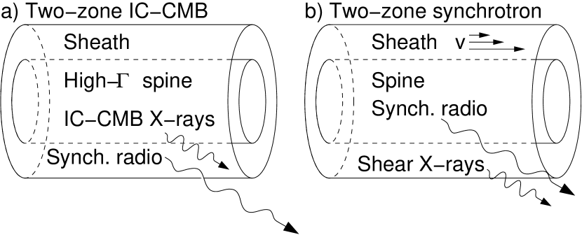
Figure 4.— Illustration of two-zone emission models. In the two-zone inverse-Compton model (IC-CMB; a), the jet needs to have a highly relativistic spine ($\Gamma\approx 50-100$) to produce the X-ray emission via upscattering of cosmic microwave background photons without contributing significant radio synchrotron emission. The slower sheath produces the bulk of the radio synchrotron emission; it may or may not be moving relativistically itself. In our two-zone synchrotron model (b), there is still a fast spine surrounded by a shear layer. In this case, the bulk of the radio synchrotron emission is produced in the spine. In the sheath, the velocity shear allows particle acceleration to take place, producing X-ray emission also by the synchrotron process (labelled “Shear X-rays”; shear acceleration may also occur in the IC-CMB model, but is not essential there). The two-zone synchrotron model would admit a much lower bulk Lorentz factor for the spine than the two-zone IC-CMB model.

In a two-zone beamed IC-CMB model for 3C 273, the highly relativistic part of the flow (the “spine”) would account for the bulk of the X-ray emission, while the slower part of the flow (the “sheath”) would dominate the synchrotron emission (Fig. 4 a). Thus, the observed radio spectral index of the jet is that of the sheath, with $\alpha_{\mathrm{sheath}}\approx-0.75$. To match the observed X-ray spectral index, the fast spine would need to have a synchrotron spectrum with $\alpha_{\mathrm{spine}}\approx-1$. To keep the observed radio spectral index unchanged, the spine would also need to have a much lower radio luminosity. As the inverse-Compton model requires the spine to have a large Doppler factor, the radio emission from the spine cannot be “Doppler-hidden” by having a Doppler factor much less than unity (cf. the suggestion of such Doppler hiding making the jet in 3C 353 edge-brightened; Swain et al., 1998). Instead, the spine has to have a much lower radio brightness than the sheath. If the spine has an (observer-frame) flux density at 1.6 GHz of 10% of that of the sheath, its steeper-spectrum contribution would not change the total spectral index between 1.6 GHz and 330 MHz by more than 0.05, i.e., within the spectral index errors. Hence, we consider a 10% contribution at 1.6 GHz the maximum plausible flux density of the spine that would keep it undetectable as a separate steep-spectrum component.

Estimating the bulk Lorentz factor

We can now estimate the bulk Lorentz factors within a 2-zone model from the X-ray:radio ratio. The X-ray emission has to be produced in the spine via upscattering of CMB photons by an electron distribution that would contribute only about 1% of the jet’s total synchrotron luminosity (where the latter is inferred from the radio flux). We just estimated that the spine could contribute at most 10% of the radio flux density at 1.6 GHz; by extrapolating the X-ray flux density to 1.6 GHz using the observed spectral index, we obtain that the X-ray:radio ratio for the spine ($R(1)$ in the notation of Harris & Krawczynski, 2002) is of order 2000. This is much larger than the value $R(1)\approx 1$ inferred from the jet’s total radio emission (Harris & Krawczynski, 2002). Following the method presented by Harris & Krawczynski (2002), we can infer the likely Doppler and Lorentz factors for the spine if we have an estimate of the magnetic field. If there is equipartition of energy between the magnetic field and the particles in both the spine and the sheath, we can use the scaling of the minimum-energy field $B_{\mathrm{min}}$ with source luminosity $L$, volume $V$ and Doppler factor $\delta$ to estimate the relative magnetic flux densities. In this case, $B_{\mathrm{min}}\propto(L/V)^{2/7}\delta^{-5/7}$ (Stawarz et al., 2003, equation A7) is the appropriate scaling; with our estimate that the spine has a total synchrotron luminosity of about 1% of that of the sheath, and assuming that the spine occupies $1/2$ of the jet diameter and hence $1/3$ of the sheath’s volume, the magnetic field in the spine would still be $\delta_{\mathrm{rel}}^{-5/7}\times$ 20% of the sheath’s (where $\delta_{\mathrm{rel}}=\delta_{\mathrm{spine}}/\delta_{\mathrm{sheath}}$ is the relative relativistic Doppler factor of spine and sheath (Georganopoulos & Kazanas, 2003)). Hence, following Harris & Krawczynski (2002), we obtain that the bulk $\Gamma_{\mathrm{spine}}$ would have to be of order 50–100 to produce $R(1)=2000$.

Jet deceleration in a two-zone IC-CMB model

The synchrotron emission from the sheath will appear boosted in the frame of the spine, thus providing an additional seed photon field for Compton scattering (Ghisellini et al., 2005). Depending on the relative sizes and speeds of spine and sheath, the energy density of the sheath photon field as perceived in the frame of the spine could be comparable to that of the cosmic microwave background. If this was the case, the boosted CMB would need to contribute only half of the seed-photon energy density. As the boosted CMB energy density scales like $\Gamma^{2}$, the required bulk Lorentz factor would be reduced only by about $1/\sqrt{2}$. At the same time, the sheath electrons will upscatter seed photons from the spine, creating an additional IC component. In the case of 3C 273, the dominant contribution to the synchrotron luminosity would arise in the sheath (“layer” in the terminology of Ghisellini et al., 2005) rather than the spine as assumed for the blazars considered by Ghisellini et al. (2005). This additional “mutual-Compton” (MC) scattering will produce detailed SEDs that are quite different from those arising in a one-zone synchrotron + beamed IC-CMB model. As noted by Ghisellini et al. (2005), the MC scattering could cause a deceleration of the spine (an “inverse Compton-rocket” effect). This might provide a more natural explanation for the deceleration that is necessary to account for the changing X-ray:radio ratios along some extragalactic jets, including 3C 273’s (see Hardcastle, 2006 and in particular Marshall et al., 2005a for the deceleration of this jet implied by a one-zone beamed-IC model). The FR I flow modeling by Laing & Bridle (2004); Canvin & Laing (2004); Canvin et al. (2005) shows that these jets decollimate as they decelerate, presumably by entrainment, while no sign of decollimation is observed in 3C 273 and other high-power jets.

However, as noted by Ghisellini et al. (2005), the large number of free parameters of this kind of two-zone model makes it very difficult to obtain definite predictions for the expected shape of the SED. The most stringent observational constraints will be imposed by verifying whether or not the radio spectrum shows any signs of the steeper-spectrum component assumed to arise in the spine at lower frequencies than observed so far, e.g., in the frequency range around 100 MHz that will soon be accessible with the Low-Frequency Array (LOFAR). In any case, the two-zone IC-CMB model requires that the “spine-sheath” jet should develop very different low-energy electron populations in the different parts of the flow. This may seem somewhat artificial if the velocity structure arises from simple velocity shear, unless the shape of the electron energy distribution in jets is governed entirely by a distributed acceleration mechanism, rather than by shock acceleration in the innermost part of the jet (compare the discussion of “shock-like” versus “jet-like” acceleration in Meisenheimer et al., 1997). The different energy distributions might arise more naturally if the two-zone flow existed from the outset (e.g., as in the model by Sol et al., 1989). A detailed parameter study is necessary to explore the range of plausible total SEDs (including synchrotron emission, beamed IC-CMB, and MC scattering); this is beyond the scope of this paper.

Constraints on two-zone models from the jet morphology

We will present a detailed study of the X-ray morphology based on the new data in a separate paper; the most relevant finding so far is that most of the jet is now clearly resolved transversely even at the Chandra resolution. However, the limit to the width of the brightness peaks in knots A and B2 is smaller than the measured sizes in the optical and radio bands (Marshall et al., 2005a), where they are clearly resolved (Bahcall et al., 1995; Jester et al., 2001, 2005). This is incompatible with the beamed IC-CMB model — even in a decelerating one-zone flow such as that considered by Georganopoulos & Kazanas, 2004, the optical emission should be the most concentrated because the “optical synchrotron” electrons have the shortest synchrotron loss scales. Thus, even though the SED of knot A admits a one-zone IC-CMB model, its morphology does not. In general, the presence of unresolved knot emission superimposed on resolved more diffuse jet emission compels us to consider two-zone models (although not necessarily only spine-sheath models).

In summary, if FR II jets have a spine-sheath structure, and the spine is highly relativistic, there will naturally be two zones in the jet with different IC-CMB emission. The “mutual-Compton” scattering of the radiation from the one zone by electrons in the other might provide a natural explanation for the apparent deceleration of 3C 273 implied by the changing X-ray:radio ratio (Ghisellini et al., 2005; Hardcastle, 2006). However, a two-zone IC-CMB model appears to require unrealistically large bulk Lorentz factors for the spine of the jet, of order 50–100. Moreover, the two-zone IC-CMB model does not intuitively explain why the emission in the X-ray band has a softer spectrum than that in the radio band.

4.2. Viability of the synchrotron model

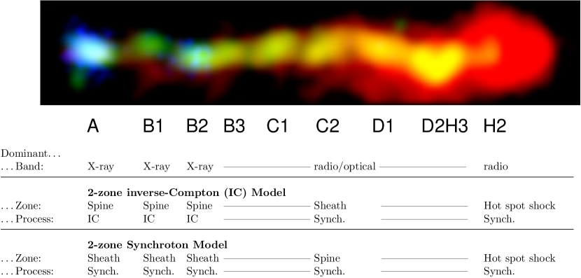
Figure 5.— False-color image of the jet in 3C273, made by sampling the individual images in Fig. 1 on a finer pixel grid, combining them to an RGB composite (blue channel: Chandra, green channel: HST, red channel: VLA) and smoothing slightly after combination to remove the sharp boundaries between the original pixels. The energetically dominant waveband is given below the knots (compare Fig. 2), as well as the dominant spatial component and corresponding emission mechanism in each of the two-zone, spine-sheath models considered in the text: a two-zone inverse-Compton model with a highly relativistic spine producing X-rays and some fraction of the optical emission via inverse-Compton scattering of CMB photons (IC-CMB), surrounded by a slower sheath producing radio synchrotron emission; and a two-zone synchrotron model in which the spine produces radio synchrotron emission, while the sheath is a shear layer that accelerates electrons emitting synchrotron X-rays. In both models, knots A and B2 may have a contribution to the X-ray emission from a different emission or acceleration mechanism.

As pointed out above, a one-zone synchrotron model is already excluded by the spectral hardening in the near-infrared/optical/UV region. Hence, we only discuss a two-zone synchrotron model here. The evidence in favor of a spine-sheath structure in FR II jets summarized in § 4.1.2 is of course equally relevant to the discussion of a two-zone synchrotron model.

In a two-zone synchrotron model, there would be the same need to account for these different electron energy distributions, but the difference would now be between the low-energy electron distribution of one zone (emitting at radio wavelengths) and the high-energy electron distribution of the other one (producing X-rays). It is already known that many low-power jets emit synchrotron X-rays (Worrall et al., 2001), and possibly all such jets do (Hardcastle et al., 2002). The extremely short synchrotron loss timescales of 10s of years for the X-ray emitting electrons require an in-situ acceleration process to generate these electrons. It would then be an obvious assumption that high-power jets are also able to accelerate such electrons. Indeed, some high-power jets show evidence for synchrotron X-ray emission (Sambruna et al., 2004; Kraft et al., 2005; Hardcastle & Croston, 2005). Moreover, Stawarz & Ostrowski (2002), Rieger & Mannheim (2002) and Rieger & Duffy (2004) have all argued that efficient particle acceleration is possible in regions of velocity shear. Thus, particle acceleration in a sheared region of the flow might provide a direct physical link between a two-zone velocity structure and a two-component synchrotron spectrum, since an additional acceleration mechanism would be available in the sheared part of the flow. We stress that the presence of shear acceleration does not preclude the possibility that there is another distributed acceleration mechanism acting in the other, or both, fluid zones, e.g., one related to the dissipation of magnetic fields (Litvinenko, 1999)

In the context of such a model, the soft X-ray spectrum in 3C 273 with $\alpha\approx-1$ for regions B2 and beyond could be caused either by a soft energy spectrum being generated by the distributed acceleration process, or because it arises from a loss-dominated part of the energy distribution. The difference in X-ray spectral index between the first bright knot A and the faint bridge B1 on the one hand, and the second bright knot B2 and beyond on the other hand, would require at least some difference of the physical parameters (either by producing a different electron energy distribution, or by producing stronger cooling), and perhaps even a different acceleration mechanism acting there. This physical difference might have been expected given that A is the first bright region of the optical and X-ray jet, after a gap of 12″ with only very faint optical (Martel et al., 2003) and X-ray (Marshall et al., 2001) emission. The difference between A and B2 may well be related to the reason for the jet lighting up at A. We will revisit the emission from the inner part of the jet in a forthcoming paper on the X-ray morphology.

In figure 5, we give a summary of the energetically dominant wavebands and the associated spatial component and emission mechanism, both for the two-zone inverse-Compton and the synchrotron model.

5. Summary and outlook

We have presented new deep Chandra Acis-S3 observations of the jet in 3C 273 and analyzed them in conjunction with archival data, concentrating on the shape of the radio / optical / X-ray SED in this paper. Fitting power laws to the radio and X-ray spectra, we find that a single-zone beamed IC-CMB model for the X-ray emission is viable only in regions A and B1; in the remainder of the jet, the X-ray spectra are softer than the radio spectra. This is in contrast with the similarly well-studied X-ray jets of PKS 0637$-$752, 1136$-$135, and 1150$+$497, where the radio and X-ray slopes are compatible with each other in all parts of the jet where both have been measured (Chartas et al., 2000; Sambruna et al., 2006). Thus, most of the X-ray emission from the jet in 3C 273 must be due to a different emission process than Compton scattering of CMB photons by the same electrons producing the bulk of the synchrotron radio emission.

A single-zone synchrotron model extending from radio to X-rays had already been ruled out for all parts of the jet based on previous observations (Röser et al., 2000; Sambruna et al., 2001; Marshall et al., 2001; Jester et al., 2002). A two-zone beamed IC-CMB model does not seem capable of accounting for the X-ray emission from 3C 273’s jet with any fewer assumptions than a two-zone synchrotron model. A two-zone IC-CMB model may still be viable, but would require extreme bulk Lorentz factors to produce the observed X-ray emission from much fewer electrons than inferred from the jet’s total radio synchrotron emission. In addition, there is no intuitive explanation for obtaining different electron energy distributions in the spine and the sheath. By contrast, a two-zone synchrotron model, in which a distributed particle acceleration mechanism related to velocity shear is producing the X-ray emitting particles, provides a causal relationship between the difference in fluid velocities and the different spectral properties. There would still be velocity and hence beaming differences between the two zones, but they would not have to be as extreme as in the two-zone IC-CMB models, and therefore one might hope to obtain better-constrained parameters for the two zones, and hence falsifiable predictions of this model. An X-ray polarimeter would enable significant progress to be made in this question; also, the mid-infrared wavelength region that has now been made accessible by the Spitzer Space Telescope will be of great importance, as shown by the analysis of this jet’s mid-infrared emission by Uchiyama et al. (2006).

It would clearly be desirable to test the consistency of the radio and X-ray spectral indices with the one-zone beamed IC-CMB model for more jets in the future. We will present a detailed analysis of the X-ray morphology of 3C 273’s jet elsewhere (for first results, see Marshall et al., 2005a). This will allow more tests of both emission models for the X-rays. In particular, understanding how the (mostly) wavelength-independent morphology of this and other jets is produced will provide crucial insights into both emission and particle acceleration mechanisms acting in this and other jets.

References

- Albert et al. (1993) Albert, C. E., Blades, J. C., Morton, D. C., Lockman, F. J., Proulx, M., & Ferrarese, L. 1993, ApJS, 88, 81
- Attridge et al. (1999) Attridge, J. M., Roberts, D. H., & Wardle, J. F. C. 1999, ApJ, 518, L87
- Bahcall et al. (1995) Bahcall, J. N., Kirhakos, S., Schneider, D. P., et al. 1995, ApJ, 452, L91
- Canvin & Laing (2004) Canvin, J. R., & Laing, R. A. 2004, MNRAS, 350, 1342
- Canvin et al. (2005) Canvin, J. R., Laing, R. A., Bridle, A. H., & Cotton, W. D. 2005, MNRAS, 363, 1223
- Capetti et al. (2002) Capetti, A., Celotti, A., Chiaberge, M., de Ruiter, H. R., Fanti, R., Morganti, R., & Parma, P. 2002, A&A, 383, 104
- Celotti et al. (2001) Celotti, A., Ghisellini, G., & Chiaberge, M. 2001, MNRAS, 321, L1
- Chandra X-ray Center (2005a) Chandra X-ray Center. 2005a, Chandra Proposers’ Observatory Guide v.8, http://cxc.harvard.edu/proposer/POG/
- Chandra X-ray Center (2005b) —. 2005b, Sherpa Reference Manual for CIAO v3.3, section 6, http://asc.harvard.edu/sherpa/documents/manuals/html/refstats.html
- Chartas et al. (2000) Chartas, G., Worrall, D. M., Birkinshaw, M., et al. 2000, ApJ, 542, 655
- Conway et al. (1993) Conway, R. G., Garrington, S. T., Perley, R. A., & Biretta, J. A. 1993, A&A, 267, 347
- Davis (2001) Davis, J. E. 2001, ApJ, 562, 575
- Falcke et al. (2004) Falcke, H., Körding, E., & Markoff, S. 2004, A&A, 414, 895
- Fanaroff & Riley (1974) Fanaroff, B. L., & Riley, J. M. 1974, MNRAS, 167, 31P
- Fender et al. (2004) Fender, R. P., Belloni, T. M., & Gallo, E. 2004, MNRAS, 355, 1105
- Fleishman (2006) Fleishman, G. D. 2006, MNRAS, 365, L11
- Freeman et al. (2001) Freeman, P., Doe, S., & Siemiginowska, A. 2001, in Proc. SPIE, Vol. 4477, Astronomical Data Analysis, ed. J.-L. Starck & F. D. Murtagh, 76
- Georganopoulos & Kazanas (2003) Georganopoulos, M., & Kazanas, D. 2003, ApJ, 594, L27
- Georganopoulos & Kazanas (2004) —. 2004, ApJ, 604, L81
- Ghisellini et al. (2005) Ghisellini, G., Tavecchio, F., & Chiaberge, M. 2005, A&A, 432, 401
- Hardcastle (2006) Hardcastle, M. J. 2006, MNRAS, 134
- Hardcastle & Croston (2005) Hardcastle, M. J., & Croston, J. H. 2005, MNRAS, 363, 649
- Hardcastle et al. (2002) Hardcastle, M. J., Worrall, D. M., Birkinshaw, M., Laing, R. A., & Bridle, A. H. 2002, MNRAS, 334, 182
- Harris & Krawczynski (2002) Harris, D., & Krawczynski, H. 2002, ApJ, 565, 244
- Harris et al. (1999) Harris, D. E., Hjorth, J., Sadun, A. C., Silverman, J. D., & Vestergaard, M. 1999, ApJ, 518, 213
- Harris et al. (2004) Harris, D. E., Mossman, A. E., & Walker, R. C. 2004, ApJ, 615, 161
- Harris & Stern (1987) Harris, D. E., & Stern, C. P. 1987, ApJ, 313, 136
- Jester et al. (2002) Jester, S., Röser, H.-J., Meisenheimer, K., & Perley, R. 2002, A&A, 385, L27
- Jester et al. (2005) Jester, S., Röser, H.-J., Meisenheimer, K., & Perley, R. 2005, A&A, 431, 477
- Jester et al. (2001) Jester, S., Röser, H.-J., Meisenheimer, K., Perley, R., & Conway, R. G. 2001, A&A, 373, 447
- Kataoka & Stawarz (2005) Kataoka, J., & Stawarz, Ł. 2005, ApJ, 622, 797
- Kraft et al. (2005) Kraft, R. P., Hardcastle, M. J., Worrall, D. M., & Murray, S. S. 2005, ApJ, 622, 149
- Laing & Bridle (2004) Laing, R. A., & Bridle, A. H. 2004, MNRAS, 348, 1459
- Lelievre et al. (1984) Lelievre, G., Nieto, J.-L., Horville, D., Renard, L., & Servan, B. 1984, A&A, 138, 49
- Litvinenko (1999) Litvinenko, Y. E. 1999, A&A, 349, 685
- Marshall et al. (2001) Marshall, H. L., et al. 2001, ApJ, 549, L167
- Marshall et al. (2005a) Marshall, H. L., Jester, S., Harris, D. E., & Meisenheimer, K. 2005a, in The X-ray Universe 2005, San Lorenzo de El Escorial [astro-ph/0511145]
- Marshall et al. (2005b) Marshall, H. L., et al. 2005b, ApJS, 156, 13
- Marshall et al. (2004) Marshall, H. L., Tennant, A., Grant, C. E., Hitchcock, A. P., O’Dell, S. L., & Plucinsky, P. P. 2004, in Proceedings of the SPIE, Vol. 5165, X-Ray and Gamma-Ray Instrumentation for Astronomy XIII, ed. K. A. Flanagan & O. H. W. Siegmund, 497–508
- Martel et al. (2003) Martel, A. R., et al. 2003, AJ, 125, 2964
- McHardy et al. (1999) McHardy, I., Lawson, A., Newsam, A., Marscher, A., Robson, I., & Stevens, J. 1999, MNRAS, 310, 571
- Meier (2002) Meier, D. L. 2002, New Astronomy Review, 46, 247
- Meisenheimer et al. (1997) Meisenheimer, K., Yates, M. G., & Röser, H.-J. 1997, A&A, 325, 57
- Merloni et al. (2003) Merloni, A., Heinz, S., & di Matteo, T. 2003, MNRAS, 345, 1057
- Perlman et al. (1999) Perlman, E. S., Biretta, J. A., Zhou, F., Sparks, W. B., & Macchetto, F. D. 1999, AJ, 117, 2185
- Pushkarev et al. (2005) Pushkarev, A. B., Gabuzda, D. C., Vetukhnovskaya, Y. N., & Yakimov, V. E. 2005, MNRAS, 356, 859
- Rieger & Duffy (2004) Rieger, F. M., & Duffy, P. 2004, ApJ, 617, 155
- Rieger & Mannheim (2002) Rieger, F. M., & Mannheim, K. 2002, A&A, 396, 833
- Röser et al. (1996) Röser, H.-J., Conway, R. G., & Meisenheimer, K. 1996, A&A, 314, 414
- Röser & Meisenheimer (1991) Röser, H.-J., & Meisenheimer, K. 1991, A&A, 252, 458
- Röser et al. (2000) Röser, H.-J., Meisenheimer, K., Neumann, M., Conway, R. G., & Perley, R. A. 2000, A&A, 360, 99
- Sambruna et al. (2004) Sambruna, R. M., Gambill, J. K., Maraschi, L., Tavecchio, F., Cerutti, R., Cheung, C. C., Urry, C. M., & Chartas, G. 2004, ApJ, 608, 698
- Sambruna et al. (2006) Sambruna, R. M., Gliozzi, M., Donato, D., Maraschi, L., Tavecchio, F., Cheung, C. C., Urry, C. M., & Wardle, J. F. C. 2006, ApJ, 641, 717
- Sambruna et al. (2001) Sambruna, R. M., Urry, C. M., Tavecchio, F., et al. 2001, ApJ, 549, L161
- Schwartz (2002) Schwartz, D. A. 2002, ApJ, 569, L23
- Schwartz et al. (2000) Schwartz, D. A., Marshall, H. L., Lovell, J. E. J., et al. 2000, ApJ, 540, L69
- Sol et al. (1989) Sol, H., Pelletier, G., & Asseo, E. 1989, MNRAS, 237, 411
- Stawarz & Ostrowski (2002) Stawarz, Ł., & Ostrowski, M. 2002, ApJ, 578, 763
- Stawarz et al. (2003) Stawarz, Ł., Sikora, M., & Ostrowski, M. 2003, ApJ, 597, 186
- Swain et al. (1998) Swain, M. R., Bridle, A. H., & Baum, S. A. 1998, ApJ, 507, L29
- Tavecchio et al. (2000) Tavecchio, F., Maraschi, L., Sambruna, R. M., & Urry, C. M. 2000, ApJ, 544, L23
- Uchiyama et al. (2006) Uchiyama, Y., et al. 2006, ApJ, in press [astro-ph/0605530]
- Willingale (1981) Willingale, R. 1981, MNRAS, 194, 359
- Worrall et al. (2001) Worrall, D. M., Birkinshaw, M., & Hardcastle, M. J. 2001, MNRAS, 326, L7