Nonlinear Development of Thermal Instability without External Forcing

Abstract

Supersonic turbulent motions are the remarkable properties of interstellar medium. Previous numerical simulations have demonstrated that the thermal instability in a shock-compressed layer produces the supersonic turbulent motion that does not decay. In this paper we focus on two- and three-dimensional numerical simulations of the non-linear development of simple thermal instability incorporating physical viscosity but without any external forcing, in order to isolate the effects of various processes responsible for the long-lasting turbulent motion. As the initial condition for our simulations, we set up spatially uniform gas with thermally unstable temperature in a box with periodic boundaries. After the linear growth stage of the thermal instability, two-phase medium forms where cold clumps are embedded in warm medium, and turbulent fluid flow clearly visible as translational motions of the cold clumps does not decay in a viscous dissipation timescale. The amplitude of the turbulent velocity increases when we reduce the Prandtl number that is the non-dimensional ratio of kinetic viscosity to thermal conduction: the saturation amplitude does not change when we increase the viscosity and thermal conduction coefficients simultaneously in order to keep the Prandtl number. This shows that the thermal conduction plays an important role in maintaining turbulent motions against viscous dissipation. The amplitude also increases when we increase the ratio of the computational domain length $L$ to the cooling length $\lambda_{\rm c}$ that is defined by the product of the cooling time and the sound speed, as long as $L\lesssim 100\lambda_{\rm c}$.

1 Introduction

The interstellar medium (ISM) is observed to be highly turbulent (Heiles & Troland 2003). Turbulence may play an important role in the subsequent evolution of ISM such as the formation of dense molecular clouds (e.g., Mac Low & Klessen 2004). A number of hydrodynamical processes have been proposed as a mechanism for generating turbulent motions in multi-phase ISM: supernova explosions (e.g., de Avillez & Mac Low 2002), Galactic differential rotation (e.g., Wada & Norman 2001), MRI (e.g., Piontek & Ostriker 2004), and winds from young stars in active star forming clouds (e.g., Li & Nakamura 2006). Among them, energetics argument favors supernova explosions as the most efficient ultimate source of turbulence (e.g., Mac Low & Klessen 2004).

When the ISM is swept-up by a compressional wave, the gas temperature in the shock-compressed gas once increases by shock-heating but eventually decreases because of higher cooling rate in compressed gas. If the temperature goes down from 6,000 K to 300 K, the gas becomes thermally unstable (Field, Goldsmith & Habing 1969; Wolfire et al. 1995, 2003). The nonlinear evolution of thermal instability (TI) in this situation has been studied by Koyama & Inutsuka (2002, hereafter KI02; Inutsuka & Koyama 2002; Inutsuka & Koyama 2004). They have found that TI generates supersonic turbulence which does not decay as long as the shock wave continues its propagation. In similar context, formation of cold clouds in warm turbulent colliding flows is also analyzed by Audit & Hennebelle (2005), Heitsch et al. (2005) and Vázquez-Semadeni et al. (2006).

In contrast to KI02, many numerical studies on compressible turbulence of hydro- and magnetohydrodynamics in one-phase medium (i.e., isothermal gas) have shown that the kinetic energy decays within a crossing time or less (Stone, Ostriker & Gammie 1998, Mac Low, Klessen & Burkert 1998, Cho & Lazarian 2004). In case of MHD simulations of supersonic turbulence, about half of energy is dissipated by shocks and the rest of it is dissipated by physical or numerical viscosity. Decaying turbulence in two-phase medium is also reported by Kritsuk & Norman (2002). They have reported a decay rate of TI-induced turbulence that is similar to that of one-phase.

In order to clarify the importance of TI in the turbulent ISM, it is imperative to understand why TI-induced turbulence in KI02 does not show rapid decay. One obvious reason is due to continuous supply of unstable gas into the post-shock region from the upwind flow. In other words, TI in the shock propagating model is continously happening in “fresh” thermally unstable gas that is continuously provided by shock compression and heating. Another aspect of the shock propagation model is that a supersonic motion of CNM does not mean supersonic with respect to WNM because two phases have very different sound speeds. A cold gas clump that has a subsonic velocity with respect to WNM can survive shock dissipation in surrounding WNM. Piontek & Ostriker (2004) have found long-lasting subsonic turbulence driven by TI, but have not treated the effect of physical viscosity that is important in this subsonic turbulence as shown below.

In this paper, we study the dissipation mechanism in TI-induced turbulence by performing two- and three-dimensional hydrodynamical simulations with realistic cooling/heating rates, thermal conduction, and physical viscosity. For the sake of simplicity, magnetic field and self-gravity are not included in this study. Numerical models and methods are described in §2. In §3, we demonstrate the kinetic properties of two-phase medium. In §4, we discuss the implications of our results. Finally, we summarize our findings in §5.

2 Numerical Methods

We solve the following compressible Navier-Stokes equations with cooling and heating terms:

$$\frac{\partial\rho}{\partial t} + \frac{\partial}{\partial x_{j}}(\rho u_{j})=0,$$ (1)

$$\frac{\partial\rho u_{i}}{\partial t} + \frac{\partial}{\partial x_{j}}(\rho u_{i}u_{j}-\sigma_{ij})=-\frac{\partial P}{\partial x_{i}},$$ (2)

$$\frac{\partial E}{\partial t} + \frac{\partial}{\partial x_{j}}\left[(E+P)u_{j}-\sigma_{ij}u_{i}-K\frac{\partial T}{\partial x_{j}}\right]$$ (3)

$$=n\Gamma-n^{2}\Lambda(T),$$

$$E = \frac{P}{\gamma-1}+\frac{\rho u_{k}u_{k}}{2},$$ (4)

$$P = nk_{\rm B}T,$$ (5)

$$n = \rho/m_{\rm H},$$ (6)

$$\sigma_{ij} = \mu\left\{\left(\frac{\partial u_{i}}{\partial x_{j}}+\frac{\partial u_{j}}{\partial x_{i}}\right)-\frac{2}{3}\delta_{ij}\frac{\partial u_{k}}{\partial x_{k}}\right\}.$$ (7)

All symbols have their usual meanings.

We take the realistic cooling function $\Lambda(T)$,

$$\frac{\Lambda(T)}{\Gamma}=1.0\times 10^{7}\exp(-1.184\times 10^{5}/(T+1000))+14\times 10^{-3}\sqrt{T}\exp(-92/T)$$ (8)

and the density independent heating rate $\Gamma$ from KI02. We assume the classical conduction coefficient of neutral hydrogen, $K=2.5\times 10^{3}T^{1/2}\,{\rm cm^{-1}K^{-1}s^{-1}}$ (Parker 1953) for a fiducial model. The relation between the viscosity $\mu$ and the thermal conductivity $K$ is characterized by Prandtl number:

$${\rm Pr}=\frac{\gamma}{\gamma-1}\frac{k_{\rm B}}{m_{\rm H}}\frac{\mu}{K},$$ (9)

where $\gamma$ is the ratio of specific heats, $k_{\rm B}$ is the Boltzmann constant and $m_{\rm H}$ is the mass of atomic hydrogen. Note that the Prandtl number for a neutral monoatomic gas is Pr=2/3. Throughout this paper we assume a gas consists of atomic hydrogen ($\gamma=5/3$).

We use an operator-splitting technique for solving the equations: the second-order Godunov method (van Leer 1979) for inviscid fluid part and first-order explicit time integration for cooling, heating, thermal conduction and physical viscosity parts. The conduction and viscosity operators have spatially second-order accuracy. The time step in our code is determined by the three criteria: (1) CFL condition, $\Delta t_{\rm CFL}\leq C_{\rm CFL}\Delta x/(c_{s}+|v_{i}|)$ with $C_{\rm CFL}=0.5$, (2) cooling and heating timescales, $\Delta t_{\rm cool}\leq 0.2\frac{k_{\rm B}T}{\gamma-1}{\rm min}(\frac{1}{\Gamma},\frac{1}{n\Lambda(T)})$, and (3) conduction and viscosity timescales, $\Delta t_{\rm vis}\leq 0.2{\rm min}(\frac{nk_{\rm B}}{(\gamma-1)K},\frac{\rho}{\mu})(\Delta x)^{2}=0.2\frac{nk_{\rm B}}{(\gamma-1)K}{\rm min}(1,\gamma/{\rm Pr})(\Delta x)^{2}$. We use uniform Cartesian grids with periodic boundary condition.

3 Characteristic Scales of TI

Table 1: Initial parameters and characteristic lengths for the fiducial model

Parameter	Value
$n_{0}$ (cm-3)	4.3
$T_{0}$ (K)	423
$P_{0}/k_{\rm B}$ (K cm-3)	1820
$\lambda_{\rm F}$ (pc)	0.0054
$\lambda_{m}$ (pc)	0.044
$\lambda_{c}$ (pc)	0.35

The development of TI is characterized by three length scales: the critical length scale, the cooling length, and the most unstable wavelength. We briefly summerize those length-scales in this section.

Even when the gas is thermally unstable, the thermal conduction can erase the perturbation whose wavelength is sufficiently small. In other words, there is a critical wavelength of TI called ‘Field length’ which is defined by

$$\lambda_{\rm F} = \sqrt{\frac{KT}{n^{2}\Lambda}}$$ (10)

$$= 1.4\times 10^{-2}\frac{T_{2}^{0.35}}{n}~{}{\rm pc}$$

(Field 1965) where $T_{2}=T/(10^{2}{\rm K})$. In this expression, we adopt a simple power law cooling rate (eqn. [3] in Wolfire et al. 2003). Note that this cooling rate shows a good agreement with the detailed calculations in the temperature range from 100 to 8,000 K (e.g., Wolfire et al. 1995, 2003 and Koyama & Inutsuka 2000). The thermal conduction is important in the two-phase interface region at which radiative cooling/heating balances conductive heating/cooling (Inutsuka, Koyama & Inoue 2005). Graham and Langer (1973) studied cold spherical clouds embedded in warm gas and found that small clouds can evaporate due to this conduction while ambient warm gas can condenses on large clouds. Obviously, the transition region of the two-phase interface must be resolved to correctly describe those evaporation and condensation of clouds. The thickness of this region is the order of the Field length (Begelman & McKee 1982). Therefore, the Field length should be resolved in numerical analysis of TI. We termed this criterion as the ‘Field condition’ (Koyama and Inutsuka 2004, hereafter KI04).

Next, we introduce the cooling length given by

$$\lambda_{c}=c_{s}\tau_{\rm cool} = \sqrt{\frac{\gamma k_{\rm B}T}{m_{\rm H}}}\frac{1}{\gamma-1}\frac{k_{\rm B}T}{n\Lambda}$$ (11)

$$= 0.55\frac{T_{2}^{0.7}}{n}~{}{\rm pc},$$

where $\tau_{\rm cool}$ is the cooling time and $c_{s}$ is the sound speed. In the scale smaller than this, pressure balance sets in rapidly on the sound crossing time which is less than the cooling time. In other words, the perturbation evolves almost isobarically. Alternatively, in the long-wavelength limit, the sound crossing time becomes relatively long, and radiative equilibrium sets in first. The radiative equilibrium pressure depends on the local density (see, e.g., solid line in right panel of Figure 3). This means that the density gradient produced by TI also produces pressure gradient that can produce larger dynamical motions than isobaric motions. Sánchez-salcedo et al. (2002) showed that large-scale perturbations generated large condensation flows with Mach numbers larger than 0.5, but small-scale perturbations evolved less dynamically.

Finally, we introduce the most unstable wavelength of TI which is approximately expressed by the geometric mean of the two characteristic lengths

$$\lambda_{m}\approx\sqrt{\lambda_{\rm F}\lambda_{c}}=0.088\frac{T_{2}^{0.525}}{n}~{}{\rm pc}$$ (12)

(Field 1965). Note that we have a size relation

$$\lambda_{\rm F}<\lambda_{m}<\lambda_{c},$$ (13)

where the realistic parameters are assumed. These three characteristic lengths of the fiducial model are listed in Table 1.

In order to simulate a gas flow of two-phase medium such as condensation and evaporation of clouds and evolution of a thermally unstable mode, at least the Field length $\lambda_{\rm F}$ and the most unstable wavelength $\lambda_{m}$ should be resolved. In addition, the cooling length may be important for the dynamical evolution of TI. Since $\lambda_{c}$ is about two order of magnitude larger than $\lambda_{\rm F}$, at least a few hundreds of grids per one-dimension are required to resolve those length-scales in a numerical analysis.

4 Nonlinear Evolution of TI

In this section, we investigate the development of TI, in particular, production of supersonic turbulence and energetics of two-phase turbulence.

4.1 TI-Induced Turbulence

As for initial conditions, we assume uniform gas with small isobaric density perturbations so that the development of velocity fluctuations is purely caused by TI. Figure 1 shows time evolution of the ratio of kinetic to thermal energies for the three different models. Dot-dashed line denotes the two-dimensional simulation starting with hot medium ($5\times 10^{5}$ K). The kinetic energy produced by TI exceeds thermal energy at $\sim$0.1 Myr which corresponds to a few cooling time of hot gas. This temporal turbulence eventually decays. This decay property in multiphase ISM was reported by Kritsuk & Norman (2002).

Solid and dotted lines in Figure 1 show the simulations starting with unstable one-phase medium in two- and three-dimension, respectively. This unstable initial condition is widely used for the simulation of TI (e.g., Sánchez-salcedo et al. 2002; Piontek & Ostriker 2004; KI04). We could not find any significant difference between two- and three-dimensional models. One snapshot (three-dimensional model K36L3D) is presented in Figure 2. The increasing kinetic energy attains maximum at $\sim$ 5 Myr which corresponds to a cooling time of WNM. After the linear growth stage of TI, non-linear turbulent state is established, irrespective of the difference in the initial condition. We call this dynamical equilibrium state “saturation.” In this saturated stage, the kinetic energy is about 1% of the thermal energy. It is interesting to note that these energies in the three different initial models converge on the same level. This seems that the saturation of turbulence driven by TI is one of the basic hydrodynamical property of the two-phase medium independent on the initial condition.

In order to satisfy the Field condition, We use artificially large conduction coefficients in these three models. The corresponding viscosity coefficients are determined by fixing the Prandtl number 2/3 except for Model K36L3D. The dependence of the saturation on the conduction and viscosity coefficients is described in the subsequent sections.

Figure 1: The ratio of kinetic to thermal energies. Dot-dashed line: two-dimensional model with initially hot medium (5$\times 10^{5}$ K). Solid line: two-dimension with initially unstable one-phase medium (Model K36M, see Table 2). Dotted line: same as the Model K36M but three-dimension (Model K36L3D).

Figure 2: Iso-density surface for Model K36L3D (L=36 pc). 128³ grids are used.

4.2 Fiducial Model of the TI-induced Turbulence

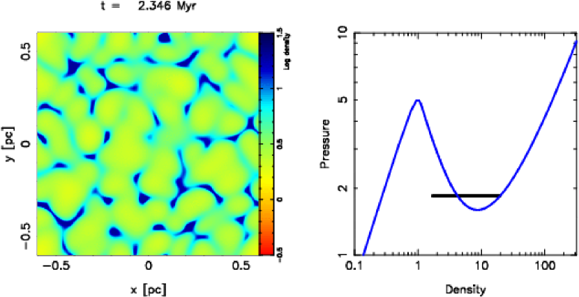
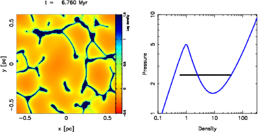
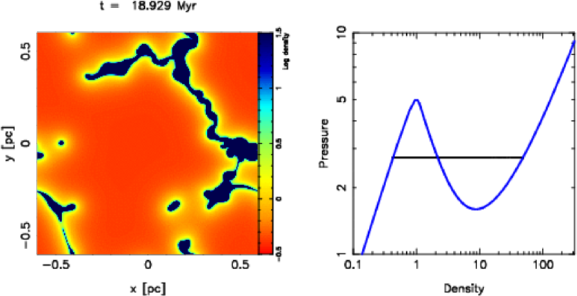
Figure 3: Evolution of TI for Model L4S (Pr=2/3, L=1.2 pc): Top: Early stage. Over density perturbations grow and reach the CNM phase while less dense perturbations have been growing toward the radiative equilibrium WNM phase. Middle: Intermediate stage. Less dense medium almost attains the radiative equilibrium WNM phase. The spatially uniform pressure evolves gradually. Bottom: Saturated stage. Small clouds evaporate and large clouds condense continuously.

Overall evolution of TI-induced turbulence in two-dimension with realistic dissipation coefficients is presented in this subsection. Initial parameters of the unperturbed state are listed in Table 1. The domain length (1.2pc) is 3.4 times larger than the cooling length $\lambda_{c}$ so that long-wavelength mode of TI can develop.

Figure 3 shows three snapshots of the density distribution alongside scatter plots of the pressure-density distribution. The radiative equilibrium curve as a function of given density is also plotted as a blue line. Top panels exhibit the early stage of the TI evolution. Initially over density regions grow and attain the equilibrium state of CNM while less density regions have not attained the WNM phase at that moment because of a longer heating timescale. Since the most unstable wavelength $\lambda_{m}$ is less than the cooling length $\lambda_{c}$, the fastest growing mode is almost isobaric: the spatially uniform pressure is nearly the same as in the initial value (see also Figure 4a).

Middle panels in Figure 3 show the stage that the dilute gas approaches the WNM phase. Toward the WNM phase, the gas must expand in order to reduce its density. Owing to the fixed volume boundaries, expanding warm gas compresses the cold dense clouds as well as warm gas itself. Consequently, the gas pressure slightly increases by forming WNM phase. The time evolution of the gas pressure is shown in Figure (4a).

Bottom panels in Figure 3 show fully developed stage of two-phase medium. Both evaporation of the small clouds and accretion of the surrounding warm gas onto the cold clouds are seen.

Since the clouds of the size smaller than $\lambda_{\rm F}$ must be erased by thermal conduction, the minimum size of cold clouds is the order of $\lambda_{\rm F}$. For those small clouds, thermal conduction provides a significant heating so that the clouds evaporate by the conductive heating. Neglecting the radiative heating and cooling terms, integration of the energy equation gives the following equation:

$$\frac{d}{dt}\int_{V}\frac{P}{\gamma-1}dV=\int_{S}K\nabla T\cdot d{\bf r}\sim S\frac{KT}{\lambda_{\rm F}},$$ (14)

where $V$ and $S$ are volume and surface of an isolated cloud, respectively. In the last part, we use the approximation that the temperature gradient is the order of $T/\lambda_{\rm F}$. This equation leads to the evaporation timescale

$$\tau_{\rm evap}\sim\frac{V}{S}\frac{P\lambda_{\rm F}}{(\gamma-1)KT}=\tau_{\rm cool}\frac{R}{2\lambda_{\rm F}}.$$ (15)

Here, we adopt cylindrical symmetry for the two-dimensional simulations, using the relation $V/S=R/2$ where $R$ is the radius of the cloud. This equation indicates that a small cloud can evaporate in a few cooling time. Detailed analysis of cloud evaporation are presented in Nagashima, Koyama & Inutsuka (2005) and Nagashima, Inutsuka & Koyama (2006).

4.3 Energy Budget and Dissipation Timescale

Figure 4a and b exhibit the time evolution of volume averaged thermal and kinetic energy, respectively. The three arrows plotted in Figure 4b correspond to the snapshots in Figure 3. The thermal energy dominates in this model. The kinetic energy does not decay but shows saturation. The kinetic energy of high density gas (Dotted line in Figure 4b) is much larger than the averaged value (Solid line).

Owing to the periodic boundary condition, the total energy $E$ (thermal plus kinetic energies per unit volume) varies only with the net heating strength. The time evolution of the total energy is given by

$$\frac{\partial}{\partial t}\langle E\rangle = \langle n\Gamma-n^{2}\Lambda(T)\rangle$$ (16)

$$= \bar{n}\Gamma-\langle n^{2}\Lambda(T)\rangle,$$

where the bracket denotes the volume average. Since we adopt the constant heating $\Gamma$ and the total mass is conserved, the total thermal energy changes according to the constant heating and the variable cooling rate $\langle n^{2}\Lambda(T)\rangle$ that depends on the local density and temperature distribution. The net heating rate, therefore, depends on the structure of the two-phase medium. Figure 4c shows the net radiative heating rate (rhs in eqn.[16]) as a function of time. The net gain rate is only on the order of 0.1 % of the constant (average) heating rate $\bar{n}\Gamma=8.6\times 10^{-26}$ ergs s^-1. In other words, departure from the overall radiative equilibrium is small.

Figure 4: Evolution of (a) thermal and (b) kinetic energies in units of 10${}^{-3}k_{\rm B}$ ergs cm^-3. Models L4S is plotted (Pr=2/3, L=1.2pc. See Table 2). Three arrows correspond to the snapshots in Figure 3. Dotted line (panel b) shows the kinetic energy of the high density gas ($\rho>\rho_{c}=4$ cm^-3). Panel c and d denote the net radiative and viscous heating in unit of $2\times 10^{-26}$ ergs s^-1, respectively. All quantities are the volume averages.

Owing to viscous dissipation, a fraction of kinetic energy continuously converts into thermal energy. The conversion rate (in two-dimension) is

$$\Phi = 2\mu\left[\left(\frac{\partial v_{x}}{\partial x}\right)^{2}+\left(\frac{\partial v_{y}}{\partial y}\right)^{2}\right]+\mu\left(\frac{\partial v_{x}}{\partial y}+\frac{\partial v_{y}}{\partial x}\right)^{2}$$ (17)

$$-\frac{2}{3}\mu\left(\frac{\partial v_{x}}{\partial x}+\frac{\partial v_{y}}{\partial y}\right)^{2}.$$

As seen in Figure 4d, dissipation rate is approximately constant after a few Myr. The dissipation timescale is estimated as $T_{diss}=\langle\rho v^{2}/2\rangle/\langle\Phi\rangle\approx 6$ Myr. Because the kinetic energy does not decrease in this timescale, we should conclude that the kinetic energy must be continously supplied by some processes. The pressure gradients, caused by the inhomogeneous cooling due to local density and temperature variation, evidently produce the translational motions. This is analyzed in §6.2.

4.4 Resolution Dependence

Figure 5: Resolution study. Thermal energy $\langle P\rangle/(\gamma-1)$ (Top) and kinetic energy $\langle\rho v^{2}\rangle/2$ (Bottom). Model L4M, L4H and L4S (512, 1024 and 2048 grids in one dimension, respectively).

The Field length $\lambda_{\rm F}$, the smallest of the three characteristic lengths of TI, should be resolved for the simulation of TI. One-dimensional numerical analysis has shown that at least the Field number, defined by $N_{\rm F}=\lambda_{\rm F}/\Delta x$, should be greater than three to achieve convergence (KI04). The fiducial two-dimensional model presented here successfully satisfies this condition by $N_{\rm F}=5.12$ where 2048 grids in one-dimension are used. In Figure 5, we superpose the results of the fiducial model with three different resolutions (i.e., 512², 1024² and 2048² grids). The corresponding Field numbers are 1.28, 2.56 and 5.12, respectively. When the Field length is moderately resolved (e.g., $N_{\rm F}$=1.28 in Model L4M, see Thin line in Figure 5), the kinetic energy is about 20 % less than that in the high resolution Model (L4S) at 25 Myr. Because of high numerical cost, we use the moderate resolution models ($N_{\rm F}\sim 1.28$) to discuss the saturation level.

5 Saturation of Turbulent Energy

In the previous section, we demonstrated that the turbulence driven by TI does not decay within a viscous dissipation timescale and shows saturation although the amplitude of the velocity in the fiducial model (Model L4S) is subsonic. It is interesting to know how large can the turbulent velocity grow. One possibility is, as Sanchez-Salcedo et al. (2000) have been pointed out, that the longer wavelength mode than cooling length $\lambda_{c}$ can develop dynamically and consequently produces large turbulent velocity. The key parameter is thus the ratio of the domain length to cooling length, $L/\lambda_{c}$ which is equivalent to the ratio of sound crossing time to cooling time. For convenience, we refer to the former definition. To understand the dependence on the ratio quantitatively, we have computed numerous models with different domain lengths $L$ and cooling length $\lambda_{c}$ that are investigated in the subsequent subsections.

Table 2: Models

Models	Resolutions	L(pc)	$k_{max}$	$\frac{\lambda_{\rm F,min}}{0.003~{}{\rm pc}}$	$N_{\rm F}$	Pr	$\frac{\lambda_{c}}{0.35~{}{\rm pc}}$	$\frac{1}{2}\langle\rho v^{2}\rangle$
L1H	256$\times$256	0.3	4	1	2.56	2/3	1	decay
L4M	512$\times$512	1.2	8	1	1.28	2/3	1	6.0e-5
L4H	1024$\times$1024	1.2	8	1	2.56	2/3	1	6.0e-5
L4S(fiducial)	2048$\times$2048	1.2	8	1	5.12	2/3	1	6.0e-5
L8M	1024$\times$1024	2.4	8	1	1.28	2/3	1	2.0e-4
L16M	2048$\times$2048	4.8	8	1	1.28	2/3	1	5.0e-4
K3M	512$\times$512	3.6	8	3	1.28	2/3	1	5.0e-4
K12M	512$\times$512	12	8	10	1.28	2/3	1	5.0e-3
K12H	1024$\times$1024	12	8	10	2.56	2/3	1	5.0e-3
K9M	128$\times$128	9	4	30	1.28	2/3	1	2.0e-3
K9M3D	128$\times$128$\times$128	9	4	30	1.28	2/3	1	2.0e-3
K36M	512$\times$512	36	8	30	1.28	2/3	1	2.0e-2
K144M	2048$\times$2048	144	16	30	1.28	2/3	1	2.0e-2
C5	512$\times$512	1.2	8	1	1.28	2/3	0.2	1.0e-3
C10	512$\times$512	1.2	8	1	1.28	2/3	0.1	4.0e-3
C30	512$\times$512	1.2	8	1	1.28	2/3	0.033	2.0e-2
K1P20	512$\times$512	1.2	8	1	1.28	0.05	1	6.0e-3
K1P100	1024$\times$1024	1.2	8	1	2.56	0.006	1	2.4e-2
K3P20	512$\times$512	3.6	8	3	1.28	0.05	1	1.5e-2
K3P100	1024$\times$1024	3.6	8	3	2.56	0.006	1	3.3e-2
K12P20	512$\times$512	12	8	10	1.28	0.05	1	2.4e-2
K12P100	1024$\times$1024	12	8	10	2.56	0.01	1	5.0e-2
K36L3D	128$\times$128$\times$128	36	4	30	0.32	0.1	1	2.0e-2
K144P100	2048$\times$2048	144	16	30	1.28	0.006	1	6.0e-2
HIM	256$\times$256	36	4	30	0.64	2/3	1	2.0e-2

5.1 Saturation Levels: Dependence on Box Size

Figure 6 shows clearly that the saturation level of the turbulent energy depends on the box size $L$: larger turbulent energy is obtained in the larger $L$ simulation. Model L1H (dotted line) having the box size of 0.3 pc shows decaying turbulence, because the box size is so small that the long-wavelength mode can not develop.

Figure 6: Box size dependence: L=0.3 pc (L1H), 1.2 pc (L4M), 2.4 pc (L8M), 4.8 pc (L16M). Pr=2/3 (see Table 1 for the initial parameters).

Figure 7 displays a snapshot of Model L16M at the late stage (see also thick line in Figure 6). The box size in this model has four times as large as in Model L4M (See Figure 3). The velocity dispersion of the model is 0.05 km/s which is still subsonic, indicating that the ratio $L/\lambda_{c}=4.8/0.35=13.7$ is not sufficiently large to produce large velocity dispersion. In order to satisfy the Field condition, a large number of grids are basically required to cover long-wavelength, which means high computational cost. Two attempts to overcome this difficulty are described in the next subsection.

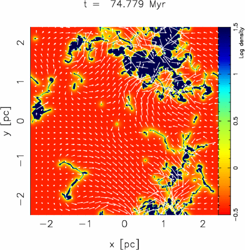
Figure 7: Snapshot: Model L16M is shown (Pr=2/3, L=4.8pc).

5.2 Saturation Levels: Role of Long-Wavelength Mode

In order to satisfy Field condition, the number of grids in one-dimension should not be less than $\sim L/\lambda_{\rm F}$. Under this constraint, artificially large $\lambda_{\rm F}$ can be used in order to reduce the grids. Piontek & Ostriker (2004) adopted similar approach with the large and temperature-independent conduction coefficient while we use the temperature-dependent coefficient, $K$. The corresponding viscosity coefficient is adopted by fixing the Prandtl number to be 2/3. In most cases, the Field condition is moderately satisfied (see Table 2).

Figure 8: Box size dependence: Large conduction and viscosity coefficients are used in order to satisfy the Field condition. Pr=2/3. L=1.2 pc (L4H), 3.6 pc (K3M), 12 pc (K12H), 36 pc (K36M) and 144pc (K144M).

Figure 8 shows the results of larger box size simulations than that in Figure 6, by using larger conduction and viscosity coefficients. The larger domain simulation shows the larger saturation amplitude. The Models K36M and K144M show the maximum saturation amplitude which is 0.3 km/s of the rms velocity. Large K run (K3M) and fiducial run (L16M) show almost the same amplitude. This indicates that the amplitude does not depend only on K.

We also present the pressure distribution in the three models (L4M, K12M, K36M) as a function of density (Figure 9). Almost uniform pressure distribution can be seen in the small box size simulation; large scatter of pressure is seen in the large box run (e.g., K36M) indicating that long-wavelength modes can generate large pressure gradients which consequently produce large turbulent velocities.

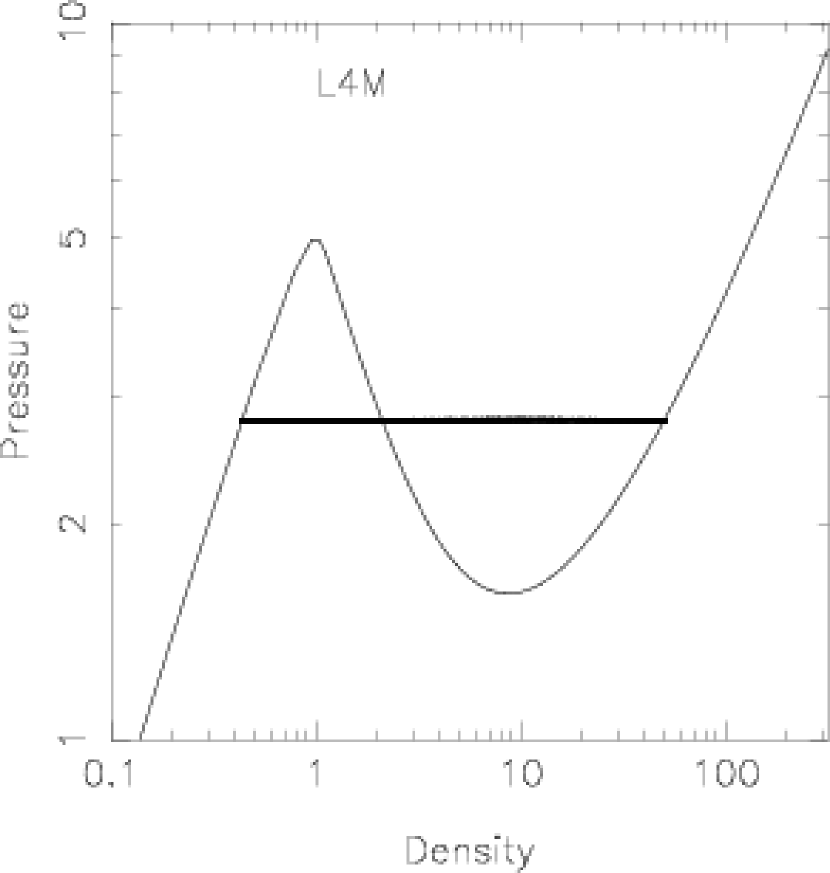
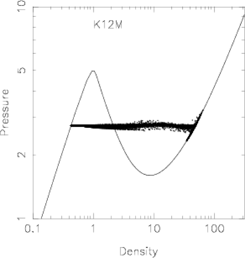
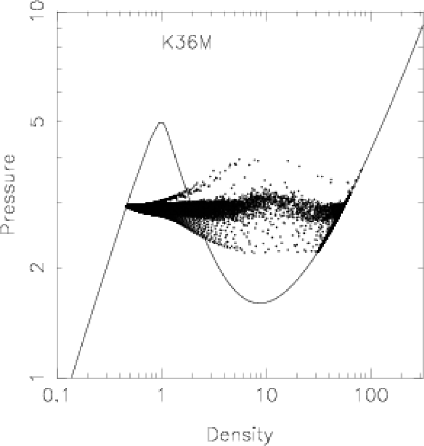
Figure 9: Pressure-density diagrams: Pr=2/3, L=1.2 pc (L4M, Left), 12 pc (K12M,Middle), 36 pc (K36M, Right). Typical late stage in each Model is plotted. Solid curves denote the thermal equilibrium state and the scatter dots are the fluid elements of all grids.

Figure 10: Saturation levels: Pr=2/3, L=1.2 pc. Models with different cooling rates are displayed (Models L4H, C5, C10, C30).

Another attempt to simulate the long-wavelength mode is to reduce the cooling length $\lambda_{c}$ by using the large cooling rate $\Lambda$ (Model C5, C10, C30, see Figure 10). In order to keep the same two-phase structure as that of fiducial model, we take the same factor for $\Gamma$ and $K$, in the following form:

$$\frac{dE}{dt}=f\left[n\Gamma-n^{2}\Lambda-K\nabla^{2}T\right]$$ (18)

where $f$ is a constant number. The results of these models show that the saturation amplitude depends on $\lambda_{c}^{-1}\propto f^{-1}$. As a conclusion, the larger amplitude are obtained in both models (larger $L$ or smaller $\lambda_{c}$).

Prandtl Number Dependence

Section 4.3 has shown that the saturation is caused by the balance between TI and viscous dissipation. This indicates that the larger amplitude will be obtained in simulations with the smaller viscosity and the larger thermal conduction coefficients. Therefore, the ratio of viscosity and conduction may be a key parameter to determine the saturation level. To show this dependence we test the models with different Prandtl number.

We have measured the saturation velocity as a function of Prandtl number using a simple form, $v\propto{\rm Pr}^{-m}$ and obtained the exponent $m$=0.15 — 0.5. The uncertainty in $m$ is mainly due to small range of Pr, $0\leq{\rm Pr}\leq 1$.

Figure 11: Saturation velocity vs length scale. Open triangle: fiducial model (L4S). Filled boxes: Model L8, L16. Filled circles: Model K9, K12, K36, K144. Open circle: K9M3D (three-dimensional simulation). Open boxes: Model C5, C10, C30. Small crosses: Model K1P20, K3P20, K12P20 (left to right). Large crosses: Model K1P100, K3P100, K12P100, K144P100 (left to right).

The saturation amplitude as a function of the ratio $L/\lambda_{c}$ is plotted in Figure 11. All the symbols except cross denote the results with Pr=2/3 showing a linear relation for $L/\lambda_{c}<100$ while they show saturation when $L/\lambda_{c}>100$. In other words, at least $100\lambda_{c}$ in length is required to obtain the efficient development of TI. Open circle denotes the result of the three-dimensional simulation (K9M3D). We could not find any significant difference between two- and three-dimensional models in terms of the saturation amplitude. The symbol cross denotes the result with smaller Prandtl number which shows the greater amplitudes than that of Pr=2/3 models.

6 Discussion

6.1 Comparison with Previous Works

It is difficult to compare the saturation levels obtained here with previous works because almost all the works did not include physical viscosity, and the amount of the numerical viscosity is unknown. In fact, Piontek & Ostriker (2004) did not include physical viscosity in their simulations that have shown similar saturated turbulence. The model parameters they used are $L$ = 100 pc and $\lambda_{c}$=1.7 pc. Simply assuming the Prandtl number to be 2/3, the velocity amplitude is expected to be 0.27 km/s from our results (Figure 11) while they measured 0.15 km/s for CNM. There may be two possible reasons for this difference. One is the numerical Prandtl number of their code that was based on ZEUS-2D may be greater than 2/3. The other is inefficient development of TI. The Field length they used, $\lambda_{\rm F}=$3.125 pc was greater than $\lambda_{c}=$1.7 pc. This means that unstable modes whose wavelength $\sim\lambda_{c}$ were suppressed owing to the thermal conduction.

Our results show that the smaller Pr simulations can achieve the larger saturation level. If the numerical method has spatially second-order accuracy, the numerical viscosity is supposed to scale as $\nu_{\rm numerical}\propto(\Delta x)^{2}$, and the numerical Prandtl number has the same dependence if the Field condition is satisfied. In this case, the saturated velocity depends on $(\Delta x)^{-0.4}$ where the exponent $m=0.2$ is assumed. Thus, the increasing of the resolution by a factor of two would give only 30 % increase in the velocity amplitude. Therefore, one tend to miss this small amplification in a numerical convergence test.

6.2 Generation Mechanism of Turbulent Motions

Physical process on the self-sustained turbulence demonstrated here may have fundamental importance as a source of turbulence in ISM. Each of CNM and WNM is thermally stable, having the similar character of decaying isothermal turbulence. Here we emphasize an essential importance of co-existence of CNM and WNM: the contrast between one- to two-phase turbulence is more remarkable in the two-phase interface. Under an assumption of (one dimensional) plane-parallel geometry, there is an unique equilibrium solution of CNM and WNM connected by the transition layer where the thermal conduction is important. This equilibrium solution can be found by solving the energy equation $\nabla\cdot K\nabla T+n\Gamma-n^{2}\Lambda=0$ with the constant pressure that is the eigenvalue of the problem (Zel’dovich & Pikelner 1969; Penston & Brown 1970). Thus, the solution can be characterized by its pressure that is called “saturation pressure.” When the pressure of the system is not the same as the saturation pressure, there is no equilibrium solution for the static two-phase medium. If $P<P_{\rm sat}$, the gas flows across the interface from CNM to WNM, and vice versa. The order of magnitude of this steady mass flow velocity is estimated by,

$$v\sim\frac{\lambda_{\rm F}}{\tau_{\rm cool}}=\frac{\gamma-1}{k_{\rm B}}\sqrt{\frac{K\Lambda}{T}}\approx 0.0018T_{2}^{0.15}~{}{\rm km/s}.$$ (19)

This velocity is lower than any saturation velocities obtained in this paper. In other words, approximate description based on the assumption of steady flow with infinite spatial extent is not sufficient to investigate self-sustained turbulence. This indicates that there might be some processes to amplify this steady-type flow. One interesting mechanism for generating those translational motions is the instability of a transition layer between WNM and CNM. An analogous instability is known in a laminar flame propagation (the so-called Darrieus-Landau instability). The detailed analysis on this instability of transition layer is shown in Inoue, Inutsuka & Koyama (2006).

7 Summary

In this work we investigate the basic hydrodynamics in interstellar two-phase medium by using two- and three-dimensional hydrodynamical simulations incorporating radiative cooling/heating, thermal conduction, and physical viscosity but without any external forcing. Starting with small amplitudes of unstable modes of thermal instability (TI), we calculate the nonlinear dynamics of the two-phase medium. Our findings are the following:

1. Saturation Property

In the fiducial model whose domain length is 1.2 pc, the kinetic energy produced by TI does not decay in at least 25 Myr which corresponds to 125 sound crossing time of WNM. On the other hand, the viscous dissipation timescale that is directly measured by the adopted viscosity term is about 6 Myr, 3 times greater than the sound crossing time of CNM. We should, therefore, conclude that the kinetic energy must be continuously supplied by some processes. These kinetic motions may be produced by pressure gradients which are caused by local inhomogeneous (density and temperature variation) cooling. As a conclusion, interstellar two-phase medium itself continuously produce turbulent motions. We call this dynamical equilibrium state “saturation.”

2. Saturation Amplitude

The saturation is observed in most of the models whose domain lengths are greater than 0.3 pc. The saturation amplitude is characterized by the ratio $L/\lambda_{c}$, where $L$ is the domain length and $\lambda_{c}$ is the cooling length defined by the product of the sound speed and the cooling time. Decaying turbulence is found in the model with $L/\lambda_{c}<1$; Self-sustained turbulence is found in the model with $L/\lambda_{c}>1$. The saturated velocity also show saturation when the ratio $L/\lambda_{c}$ is greater than 100. The maximum of the saturation velocity is about a half of the sound speed of CNM if the Prandtl number is assumed to be 2/3.

3. Numerical Resolution for TI

In order to obtain maximum saturation level of TI-induced turbulence, the computational domain length needs to be greater than $100\lambda_{c}$. On the other hands, the Field length, the minimum characteristic lengths of TI, should be resolved to avoid resolution-dependent results. Then, simulations should cover the length ranging from $\lambda_{\rm F}$ to $100\lambda_{c}$. If the realistic parameters are used, the ratio $\lambda_{c}/\lambda_{\rm F}$ is 117 and therefore the total grids per one-dimension needs $\sim 10^{4}$ which means prohibitively expensive calculation at present, in particular, for multi-dimensions. Reducing the ratio $\lambda_{c}/\lambda_{\rm F}$ by using artificial parameters demonstrated in this paper is available. However, one should meet the important criterion that $\lambda_{\rm F}$ is less than $\lambda_{c}$ in order not to suppress the most unstable mode of TI by thermal conduction.

4. Prandtl Number Dependence

The saturation amplitude of turbulent velocity does not change when we increase the viscosity and thermal conduction coefficients simultaneously in order to keep the Prandtl number. This shows that the thermal conduction plays an important role in maintaining turbulent motions against viscous dissipation. The amplitude also increases when we decrease the Prandtl number: $v\propto$Pr^-m with $m=$0.15 — 0.5.

References

- (1) Audit, E., & Hennebelle, P. 2005, A&A, 433, 1
- (2) Begelman, M. C., & McKee, C. F. 1990, ApJ, 358, 375
- (3) Cho, J., & Lazarian, A. 2004, ApJ, 615, L41
- (4) de Avillez, M. A., & Mac Low, M.-M. 2002, ApJ, 581, 1047
- (5) Field, G. B. 1965, ApJ, 142, 531
- (6) Field, G. B., Goldsmith, D. W., & Habing, H. J. 1969, ApJ, 155, L149
- (7) Graham, R., & Langer, W. D. 1973, ApJ, 179, 469
- (8) Heiles, C., & Troland, T. H. 2003, ApJ, 586, 1067
- (9) Heitsch, F., Burkert, A., Hartmann, L. W., Slyz, A. D., & Devriendt, J. E. G. 2005, ApJ, 633, L113
- (10) Inoue, T., Inutsuka, S., & Koyama, H. 2006, ApJ, submitted (astro-ph/0604564)
- (11) Inutsuka, S., & Koyama, H. 2002, Ap&SS, 281, 67
- (12) Inutsuka, S., & Koyama, H. 2004, Gravitational Collapse: From Massive Stars to Planets., RMxAC 22, 26
- (13) Inutsuka, S., Koyama, H. & Inoue, T. 2005, in MAGNETIC FIELDS IN THE UNIVERSE: From Laboratory and Stars to Primordial Structures, AIPCP 784, 318
- (14) Koyama, H., & Inutsuka, S. 2000, ApJ, 532, 980
- (15) Koyama, H., & Inutsuka, S. 2002, ApJ, 564, L97 (KI02)
- (16) Koyama, H., & Inutsuka, S. 2004, ApJ, 602, L25 (KI04)
- (17) Kritsuk, A. G., & Norman, M. L. 2002, ApJ, 569, L127
- (18) Li, Z., & Nakamura, F. 2006, ApJ, 640, L187
- (19) Mac Low, M.-M., & Klessen, R. S. 2004, Reviews of Modern Physics, 76, 125
- (20) Mac Low, M.-M., Klessen, R. S., Burkert, A., & Smith, M. D. 1998, Physical Review Letters, 80, 2754
- (21) Nagashima, M., Koyama, H., & Inutsuka, S. 2005, MNRAS, 361, L25
- (22) Nagashima, M., Inutsuka, S., & Koyama, H. 2006, ApJ, submitted (astro-ph/0603259)
- (23) Parker, E. N. 1953, ApJ, 117, 431
- (24) Penston, M. V., & Brown, F. E. 1970, MNRAS, 150, 373
- (25) Piontek, R. A., & Ostriker, E. C. 2004, ApJ, 601, 905
- (26) Stone, J. M., Ostriker, E. C., & Gammie, C. F. 1998, ApJ, 508, L99
- (27) Sánchez-Salcedo, J., Vázquez-Semadeni, E., & Gazol, A. 2002, ApJ, 577, 768
- (28) van Leer, B. 1979, J. Comp. Phys., 32, 101
- (29) Vázquez-Semadeni, E., Ryu, D., Passot, T., Gonzalez, R. F., & Gazol, A. 2006, ApJ, accepted (astro-ph/0509127)
- (30) Wada, K., & Norman, C. A. 2001, ApJ, 547, 172
- (31) Wolfire, M. G., Hollenbach, D. McKee, C. F., Tielens, A. G. G. M., & Bakes, E. L. O. 1995, ApJ, 443, 152
- (32) Wolfire, M. G., McKee, C. F., Hollenbach, D., & Tielens, A. G. G. M. 2003, ApJ, 587, 278
- (33) Zel’dovich, Y., & Pikel’ner, S., 1969, JETP, 29, 170