Shedding New Light on the 3C 273 Jet with the Spitzer Space Telescope

Abstract

We have performed infrared imaging of the jet of the quasar 3C 273 at wavelengths 3.6 and $5.8\ \mu\rm m$ with the Infrared Array Camera (IRAC) on the Spitzer Space Telescope. When combined with the radio, optical and X-ray measurements, the IRAC photometry of the X-ray-bright jet knots clearly shows that the optical emission is dominated by the high-energy emission component of the jet, not by the radio synchrotron component, as had been assumed to date. The high-energy component, represented by a power-law from the optical through X-ray, may be due to a second synchrotron component or to inverse Compton scattering of ambient photons. In the former case, we argue that the acceleration of protons exceeding energies of $E_{\rm p}\sim 10^{16}\ \rm eV$ or possibly even to $E_{\rm p}\sim 10^{19}\ \rm eV$ would be taking place in the jet knots of 3C 273 assuming that the acceleration time is proportional to the particle gyroradius. In contrast, the inverse Compton model, into which highly relativistic Doppler beaming has to be incorporated, requires very low-energy electrons of $E_{\rm e}\sim 1\ \rm MeV$ in the jet knots. The present polarization data in the radio and optical would favor the former interpretation in the case of the 3C 273 jet. Sensitive and detailed measurements of optical polarization are important to establish the radiation mechanism responsible for the high-energy emission. The present study offers new clues as to the controversial origin of the X-ray emission seen in many quasar jets.

1. Introduction

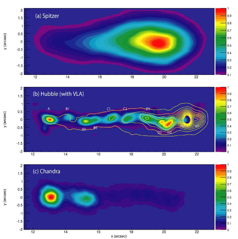
Figure 1.— Multifrequency images of the 3C 273 jet normalized to the the maximum pixel. (a) Spitzer IRAC (PSF-subtracted) image at $3.6\ \mu\rm m$; (b) HST image at 620 nm with VLA (at 2.0 cm) contours overlaid [adapted from Jester et al. (2005)]; (c) Chandra image in the 0.4–6 keV interval. The origin of the coordinate system is at the 3C 273 core and the horizontal axis, parallel to the ridge line of the jet, is set at position angle $222\arcdeg$ (the quasar is to the left at $x=0$).

Large-scale jets extending to hundreds of kiloparsec distances from the quasar nucleus often radiate their power predominantly in X-rays. This has been revealed by surveys with the Chandra X-ray Observatory (Sambruna et al., 2004; Marshall et al., 2005) following its unexpected discovery of an X-ray jet in the quasar PKS 0637$-$752 ($z=0.65$: Chartas et al., 2000; Schwartz et al., 2000). Despite extensive observational and theoretical work, the dominant X-ray emission mechanism operating in quasar jets remains unsettled (e.g., Atoyan & Dermer, 2004; Hardcastle, 2006). Neither naive single-component synchrotron nor synchrotron-self-Compton models can fully explain the spectral energy distributions (SEDs) at radio, optical and X-ray wavelengths. A widely discussed hypothesis for the strong X-ray emission is relativistically enhanced inverse Compton (IC) scattering off the cosmic microwave background (CMB) photons (Tavecchio et al., 2000; Celotti et al., 2001). In this model, the bulk velocity of the jet is assumed to be highly relativistic all the way to nearly megaparsec distances, with a Doppler factor of $\delta\sim 10$. Applying the beamed IC model to a large sample of Chandra-detected quasar jets, Kataoka & Stawarz (2005) found a range of $4\lesssim\delta\lesssim 16$ for $\sim 90\%$ of the sources.

Alternative scenarios for producing X-ray emission at such large distances from the central engine include a variety of “non-conventional” synchrotron models. The X-ray emission could be explained by a spectral hump in a synchrotron spectrum as a result of reduced IC cooling in the Klein-Nishina regime provided that a Doppler factor of the jet is large (Dermer & Atoyan, 2002). Alternatively, a second synchrotron component responsible for the X-rays could be formed by turbulent acceleration in the shear boundary layer (Stawarz & Ostrowski, 2002) or by hypothetical high-energy neutral beams (neutrons and gamma-rays) from the central engine (Atoyan & Dermer, 2001; Neronov et al., 2002). Finally, synchrotron radiation may be produced by very-high-energy protons, $E_{\rm p}\gtrsim 10^{18}\ \rm eV$ (Aharonian, 2002). Discussion of these models is hampered mostly by the limited observational windows available so far. Apart from radio observations, only Hubble Space Telescope (HST) and Chandra have the capability to resolve jets of powerful quasars.

To explore the mid-infrared properties of the extended jet emission from powerful quasars and thereby to shed new light on the riddle of the Chandra-detected jets, we performed Spitzer IRAC imaging observations of four powerful quasars during the first observing cycle. The first result of this program, based on the observation of quasar PKS 0637$-$752 (Uchiyama et al., 2005), reported the first mid-infrared detection of jet knots in a powerful quasar, and demonstrated that mid-infrared fluxes are of great importance in studying the SEDs, given the large gap between the radio and optical wavelengths. Following Georganopoulos et al. (2005), we also showed that in the context of the beamed IC model, observations with the Spitzer IRAC can constrain the matter content of jets (Uchiyama et al., 2005).

In this paper, we present Spitzer IRAC results for the well-known jet in the nearby bright quasar 3C 273. We combine Spitzer infrared measurements with available data from the Very Large Array (VLA), HST, and Chandra, forming an unprecedented data set to study the physics in extragalactic jets, not easily attainable for any of the other Chandra-detected jets found in more distant quasars. With these data we show that the multiwavelength SED can be decomposed into two distinct nonthermal components. Based on our finding, we consider plausible scenarios for the origin of the X-ray emission, and derive quantitative constraints on the physical state of the jet knots.

This paper is organized as follows. In §2 we summarize previous results on the 3C 273 jet. In §3 we present analysis of the new Spitzer IRAC data and describe the radio, optical, and X-ray data for the same emission regions. The multiwavelength spectral energy distributions are presented and discussed in §4. Concluding remarks are given in §5.

The redshift of 3C 273 is $z=0.158$ (Schmidt, 1963), so we adopt a luminosity distance of $D_{L}=749\ \rm Mpc$ (at this distance $1\arcsec$ corresponds to a linear scale of $2.7\ \rm kpc$) for a $\Lambda$CDM cosmology with $\Omega_{\rm m}=0.27$, $\Omega_{\Lambda}=0.73$, and $H_{0}=71\ \rm km\ s^{-1}\ Mpc^{-1}$ (e.g., Spergel et al., 2003). We define the spectral index, $\alpha$, in a conventional way according to the relation $f_{\nu}\propto\nu^{-\alpha}$, where $f_{\nu}$ is the flux density at frequency $\nu$.

2. A Brief Summary of the 3C 273 Jet

The presence of the kiloparsec scale jet of 3C 273 was recognized already in the famous quasar-discovery paper of Schmidt (1963). The jet of 3C 273 has been extensively studied (see Courvoisier, 1998; Stawarz, 2004, for reviews): in the radio (Davis et al., 1985; Conway et al., 1993), in the near-infrared (McLeod & Rieke, 1994; Neumann et al., 1997; Jester et al., 2005), in the optical (Röser & Meisenheimer, 1991; Bahcall et al., 1995; Jester et al., 2001, 2005), and in the X-rays (Harris & Stern, 1987; Röser et al., 2000; Marshall et al., 2001; Sambruna et al., 2001). Figure 1 shows the jet at various wavelengths (see §3.2 for details). Radio and optical emission from the large-scale jet are almost certainly synchrotron in nature given their measured polarizations and the coincidence in orientation. However, the emission mechanism giving rise to the X-rays has been controversial (see below).

The one-sided radio jet appears continuous all the way from the nucleus to the “head” region increasing in brightness toward the head (Conway et al., 1993). The head region is located $\simeq 23\arcsec$ from the nucleus or a projected distance of 62 kpc. The jet shows a sideways oscillation or “wiggle” with respect to the ridge line of the jet. The nonthermal radio spectrum is characterized by spectral index $\alpha_{\rm radio}\simeq 0.7\mbox{--}0.8$; the spectral index shows little variation along the jet. At the southeastern side the jet is accompanied by an extended but narrow “lobe” that shows a quite steep spectrum of $\alpha_{\rm radio}\sim 1.5$ (Davis et al., 1985). The faint lobe may be backflow from the hot spots or may represent outer boundary layers.

Optical imaging of the large-scale jet with HST (Bahcall et al., 1995) revealed a structured morphology that is characterized by successive bright knots interspersed by regions of weak emission. The optical jet, extending from knot A to H2, is coincident with the radio features, but the brightness profile in the optical differs from that in the radio frequencies. The optical spectra are harder in regions close to the core (Röser & Meisenheimer, 1991), in such a way that spectral index declines from $\alpha_{\rm opt}\simeq 0.6$ at knot A to $\alpha_{\rm opt}\simeq 1.5$ at D2/H3 (Jester et al., 2001). It has been demonstrated that the flux at 300 nm (near ultraviolet) shows an excess over the extrapolation from lower frequencies (Jester et al., 2002).

Both the radio and optical jet emission are linearly polarized. From $x=15\arcsec$ to $19\arcsec$ (where $x$ denotes the angular distance from the core) the degree of radio polarization is $10\mbox{--}20\%$, and the average is consistent with the optical value (Röser & Meisenheimer, 1991; Röser et al., 1996). This agreement argues that both the optical and radio emission have a common (synchrotron) origin. The inferred magnetic field is longitudinal along the ridge line of the jet out to $x\simeq 21\arcsec$, beyond which the sudden transition of the magnetic field configuration from longitudinal to transverse is observed in the polarization data in both the radio (Conway et al., 1993) and optical (Scarrott & Rolph, 1989; Röser & Meisenheimer, 1991). Based on the distinctive polarization pattern and the radiation spectrum, the head region is widely considered to harbor terminal shocks and, as such, is physically different from its upstream knots.

Excess X-ray emission associated with the jet has been reported based on observations made with EINSTEIN (Harris & Stern, 1987) and ROSAT (Röser et al., 2000). Chandra observations have confirmed the X-ray emission along the jet and allowed detailed study of its spatial and spectral properties (Sambruna et al., 2001; Marshall et al., 2001). X-ray flux is detected along the whole length of the optical jet, from $x\simeq 12\arcsec$ (knot A) to $\simeq 21\arcsec$. Regions closer to the core, specifically knots A and B2, are particularly bright in the X-ray. The X-ray spectrum shows a power-law continuum, with spectral index $\alpha_{\rm x}\simeq 0.6\mbox{--}0.9$, indicative of its nonthermal nature (Marshall et al., 2001). For knot A, a synchrotron-self-Compton (SSC) model (with an equipartition magnetic field and without Doppler beaming) predicts the SSC X-ray flux lower by three orders of magnitude than the observed flux (see Röser et al., 2000; Sambruna et al., 2001; Marshall et al., 2001).

It has been claimed that the innermost knot A has a straight power law continuum extending from the radio to X-ray, while the subsequent knots are described by a power law with a cut-off around $10^{14}$ Hz plus a separate X-ray component (Röser et al., 2000; Marshall et al., 2001). If so, the radio through X-ray emission in knot A may be ascribed to synchrotron emission from the same electrons as the radio emission; the X-rays in the other knots are then produced in some other way. On the other hand, Sambruna et al. (2001) argued that knot A as well as subsequent knots has a spectral break at optical wavelengths and suggested the SED is comprised of two components, a synchrotron part (radio to optical) and a beamed IC part (X-ray and beyond). Finally, based on deep VLA and HST observations, Jester et al. (2002) found a significant flattening in the near-infrared to ultraviolet spectra and argued that the radio-optical emission cannot be ascribed to single-population synchrotron radiation requiring an additional high-energy component (see also Jester et al., 2005). Below we construct the SEDs of the jet knots based on the extensive VLA, Spitzer, HST, and Chandra data, which allow us to elucidate the controversy in interpreting the shapes of the broadband SEDs. We then discuss possible origins for the high-energy emission, X-rays in particular.

3. Observations and Analysis

3.1. Spitzer IRAC Observation

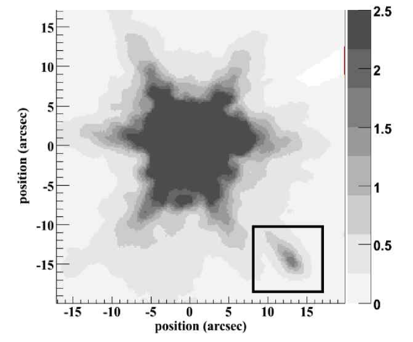
Figure 2.— Spitzer IRAC image of 3C 273 and its jet at $3.6\ \mu\rm m$ in units of $\rm MJy\ sr^{-1}$. North is up and east is to the left. The origin of the coordinates is at the quasar core. The jet emission is clearly visible in the box drawn in the lower right quadrant.

The infrared observations of 3C 273 with Spitzer IRAC were carried out on 2005 June 10 as part of our GO-1 program (Spitzer Program ID 3586). IRAC is equipped with a four-channel camera, InSb arrays at wavelengths 3.6 and $4.5\ \mu\rm m$ and Si:As arrays at 5.8 and $8.0\ \mu\rm m$, each of which has a field of view of $5\farcm 2\times 5\farcm 2$ (Fazio et al., 2004). The InSb arrays operate at $\sim 15\ \rm K$ while the Si:As arrays operate at $\sim 6\ \rm K$. Only the pair of 3.6 and $5.8\ \mu\rm m$ arrays, observing the same sky simultaneously, was chosen for our observation, to obtain longer exposures in one pair of bandpasses as opposed to two pairs with half the exposure time. The 3.6/5.8 pair was chosen because of its better spatial resolution and sensitivity. The pixel size in both arrays is $\simeq 1\farcs 22$. The point-spread functions (PSFs) are characterized by widths of $1\farcs 66$ and $1\farcs 88$ (FWHM) for the 3.6 and $5.8\ \mu\rm m$ bands, respectively (Fazio et al., 2004). The flux measurement of point sources with IRAC is calibrated to an accuracy of 2% (Reach et al., 2005).

For each IRAC band, we obtained 26 well-dithered frames, each with a 30 s integration time. The pipeline process (version S12.0.2) at the Spitzer Science Center (SSC) yielded 26 calibrated images. These calibrated frames were combined into a mosaic image with a pixel size of $0\farcs 2$ using the SSC package MOPEX (Makovoz & Marleau, 2005), which removes spurious sources such as cosmic rays and moving objects based on inter-frame comparisons. The dithered frames were combined using the “drizzling” technique (Fruchter & Hook, 2002). Finally, we made use of the astrometric positions of three field optical sources that have infrared counterparts to accurately ($\lesssim 0\farcs 2$) locate the position of 3C 273 and its jet in the IRAC image. The $3.6\ \mu\rm m$ mosaic image is shown in Fig. 2. Note that although the quasar core is extremely bright, the jet emission clearly stands out to the southwest.

As is evident from Fig. 2, the infrared emission of the jet is contaminated by the PSF wings of the bright quasar core. Therefore, measuring the infrared fluxes of the jet components requires careful removal of the wings of the core underneath the jet emission. Unlike the case of PKS 0637$-$752 (Uchiyama et al., 2005), the point-spread function provided by the SSC is not applicable for the much longer jet of 3C 273. Instead we made use of deep IRAC images of a very bright star in the Extended Chandra Deep Field South (E-CDFS) to generate a PSF template that is bright enough out to a distance of $\sim 20\arcsec$ away from the core. In fact, the template star is brighter than 3C 273 itself by a factor of $\simeq 13$ in the $3.6\ \mu\rm m$ band and by a factor of $\simeq 4$ in the $5.8\ \mu\rm m$ band, respectively. Due to the saturation in both the 3C 273 and E-CDFS images, and possible contributions from the host galaxy of 3C 273, the PSF subtraction can only be carried out reliably for $x>10\arcsec$, but fortunately it covers the entire length of the main body of the optical and X-ray jet. The PSF subtraction procedure introduces an additional systematic error in the infrared flux determination. Based on the small level of intensity due to a residual in PSF subtraction in the vicinity of the jet, we have estimated the systematic errors to be $0.05\ \rm MJy\ sr^{-1}$ for the $3.6\ \mu\rm m$ channel and $0.3\ \rm MJy\ sr^{-1}$ for the $5.8\ \mu\rm m$ channel, which are added in quadrature to the noise of each pixel when photometry is performed. The jet is so bright that photometry errors due to noise become unimportant with respect to these systematic errors.

The core emission of 3C 273 itself is saturated in both the $3.6\ \mu\rm m$ and $5.8\ \mu\rm m$ science frames. An additional frame was taken in a high-dynamic-range mode with a short integration time (1 s), such that 3C 273 itself is unsaturated; we use this frame to estimate the mid-infrared flux of the quasar core. We obtain the flux density of the 3C 273 core to be $\simeq 170$ mJy at $3.6\ \mu\rm m$ and $\simeq 230$ mJy at $5.8\ \mu\rm m$, respectively. At the relevant wavelengths, the spectrum of 3C 273 is known to have a steady small bump at $\sim 3.5\ \mu\rm m$ superposed on a variable power-law continuum (Robson et al., 1986). At the L band ($3.45\ \mu\rm m$), Türler et al. (1999) list the mean flux density of $\bar{f_{\nu}}=160.5\ \rm mJy$ with a dispersion (due to time variability) of $\sigma_{\nu}=33.5\ \rm mJy$, with which the IRAC flux is consistent. The spectroscopic observation of 3C 273 on 2004 January 6 made with the Infrared Spectrograph (IRS) on Spitzer gives the flux density of $f_{\nu}\simeq 190\ \rm mJy$ at $5.8\ \mu\rm m$ (Hao et al., 2005). The power-law continuum in June 2005 (our observation) seems slightly brighter than January 2004. It should be noted, however, that the flux estimate from a single short frame suffers from larger systematic errors as compared to the science frames.

3.2. Multiwavelength Jet Images

Figure 1a shows the IRAC image at $3.6\ \mu\rm m$ of the 3C 273 jet after subtraction of the PSF wings of the quasar core, where a line in position angle $222\arcdeg$ from the core is adopted as a reference horizontal axis. The $5.8\ \mu\rm m$ image is essentially similar to the $3.6\ \mu\rm m$ image but with slightly worse resolution. In Fig. 1, we also show high-resolution radio (at a wavelength of 2.0 cm obtained with VLA), optical (at 620 nm with HST), and X-ray (with Chandra) images. The VLA and HST images are same as those presented in Jester et al. (2005), both of which have an effective resolution (FWHM) of $0\farcs 3$. (The resolution in the HST image is artificially degraded from its native resolution to facilitate a meaningful comparison with other bands. The strongest radio spot H2 is truncated in the VLA contour map.) The Chandra image is based on new and deep observations with the ACIS-S detectors (PI: Jester). We describe the data analysis of the Chandra observations later in §3.5 [see also Jester et al. (2006, submitted) for complementary analyses]. Though the X-ray image presented here is essentially identical to Fig. 1 of Marshall et al. (2001), which was derived from the early calibration observations with the grating detectors, the spectral parameters are updated taking into account calibration improvement.

The IRAC infrared emission traces almost perfectly the main body of the optical jet; the onset of the infrared jet coincides with the innermost optical knot A centered at $x\simeq 13\arcsec$, and the infrared jet starts fading around $x\simeq 21\arcsec$ in the head region. A wiggling shape with a transverse amplitude of $\Delta y\sim 0\farcs 2$ that is evident in the optical can barely be seen in the $3.6\ \mu\rm m$ image. The infrared jet brightness shares an overall spatial pattern with the radio map in a sense that the brightness of the jet increases toward the outer part almost monotonically. However, the radio intensity peaks at H2 where the infrared jet has already started getting fainter. The overall jet in the IRAC bands looks more similar to that at the near-infrared wavelength (see Neumann et al., 1997, for a $K^{\prime}$ band image). In contrast, in the optical at 620 nm each knot is more or less of similar brightness, suggesting a spectral change from longer wavelengths.

To further investigate the jet emission quantitatively, particularly in terms of multiwavelength analysis, we derive the flux densities of individual knot components, at radio, infrared, optical, and X-ray wavelengths. The results of the photometry are summarized in Table 1, and presented in a conventional $\nu f_{\nu}$ form in Figs. 5 and 8. In the subsequent sections, we describe the methods of our measurements in each band before proceeding with multiwavelength analysis in §4.

3.3. Infrared Photometry

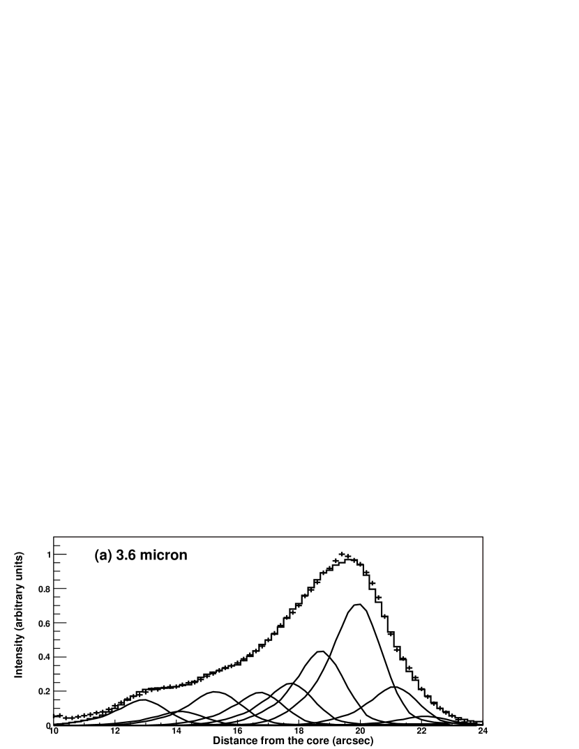
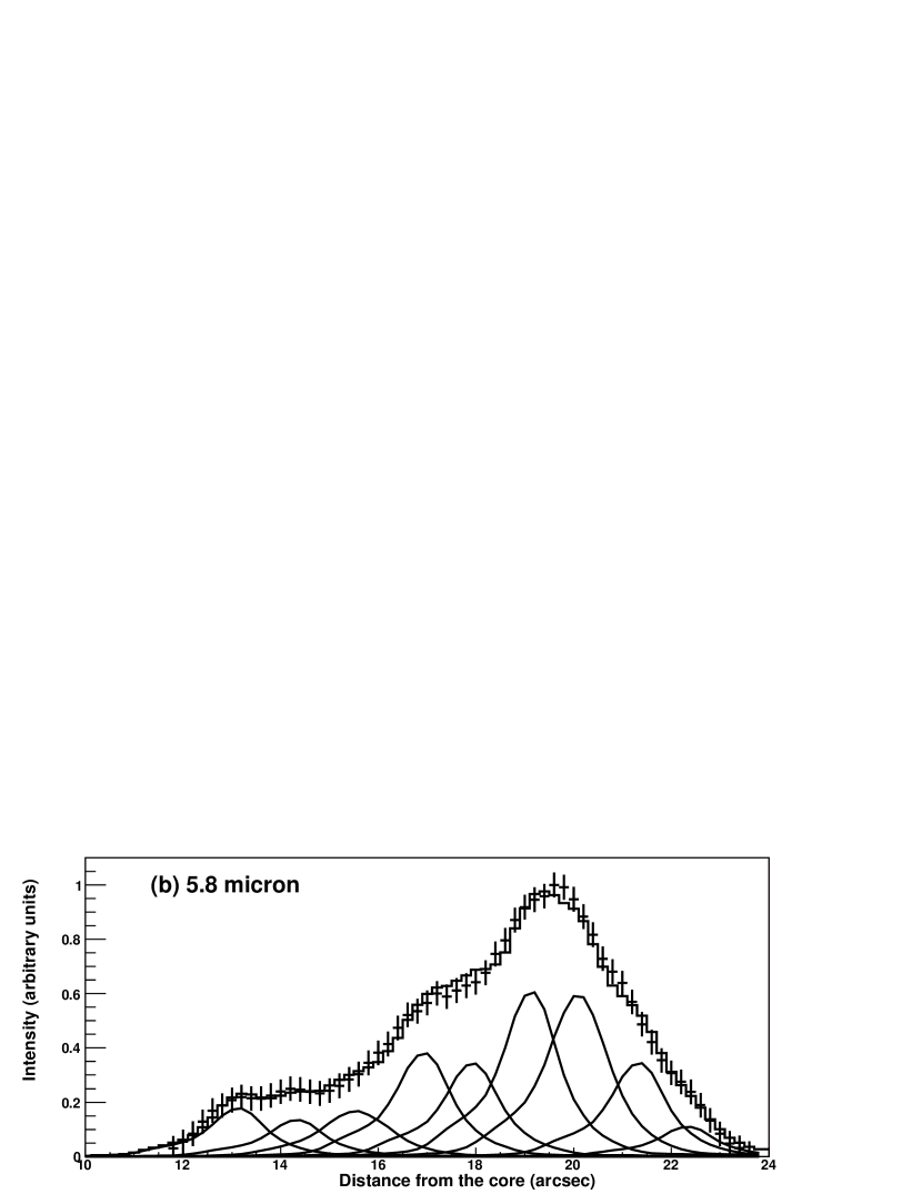
Figure 3.— Intensity profiles of the 3C 273 jet along the ridge line integrated over the vertical dimension from $-1\arcsec$ to $1\arcsec$ (a) at $3.6\ \mu\rm m$ and (b) at $5.8\ \mu\rm m$ obtained with Spitzer IRAC, together with the best-fit models comprised of 9 knot features.

Table 1Flux Densities of 3C 273 Jet Knots

	Flux Density, $f_{\nu}$
Frequency	A	B1	B2/B3	C1	C2	D1	D2/H3	H2	H1
$\nu$ (Hz)
VLA (mJy):
$8.33\times 10^{9}$	52	42	77	70	93	250	500	750	330
$1.50\times 10^{10}$	33	27	54	48	63	160	310	440	200
$2.31\times 10^{10}$	24	20	38	36	45	110	220	280	130
Spitzer ($\mu$Jy):
$5.23\times 10^{13}$	45$\pm$10	35$\pm$12	49$\pm$11	98$\pm$11	89$\pm$12	154	161	87$\pm$12	28$\pm$11
$8.45\times 10^{13}$	27	15$\pm$2.6	39	36	46	80	140	41	10$\pm$2.6
HST ($\mu$Jy):
$1.87\times 10^{14}$	7.6	4.4	11	9.0	11	21	30	5.4	1.5
$4.85\times 10^{14}$	3.6	1.7	4.0	2.6	2.5	3.6	6.2	1.1	$\cdots$
$1.00\times 10^{15}$	2.4	0.93	2.0	1.1	0.90	1.2	2.1	0.40	$\cdots$
Chandra (nJy):
$2.14\times 10^{17}$	46	11	26	5.8	5.1	6.1	7.6	$\cdots$	$\cdots$
$3.77\times 10^{17}$	28	6.2	14	2.7	2.6	3.7	3.9	$\cdots$	$\cdots$
$1.05\times 10^{18}$	12	2.7$\pm$0.3	5.1	0.9$\pm$0.2	1.1$\pm$0.2	0.9$\pm$0.2	1.4$\pm$0.3	$\cdots$	$\cdots$

Note. — The 90% errors are shown only when exceeding $10\%$. Otherwise a formal error of 10% is assigned to conservatively account for the systematic errors (see the text). The optical fluxes are corrected for Galactic extinction using $A_{V}=0.07$. The X-ray fluxes are corrected for Galactic absorption using $N_{\rm H}=1.7\times 10^{20}\ \rm cm^{-2}$.

The angular separation of adjacent knots (typically $\simeq 1\arcsec$) is comparable to the width of the IRAC PSF, which allows us to derive knot fluxes nearly individually even though the infrared images do not show discernible knots. We have modeled the two-dimensional brightness distribution of the whole length of the infrared jet with a series of PSFs of variable intensity centered on the positions of the known optical knots. We constructed the PSF based on nearby template stars. To account for possible slight variations in the widths of the PSFs by $\sim 10\%$, we adjusted each PSF width so that the PSF shape fits well the jet in the $y$-direction. As shown in Fig. 1b, 11 knots are predefined from the optical image. Among them, B2 and B3 were combined into a single component since the two knots are too close (separated only by $0\farcs 5$) to be fit individually. Similarly, D2 and H3 were united. Elongated PSFs were applied to the combined knots so as to account for the multiplicity. Whereas the optical spectra of D2 and H3 are similar to one another, the optical slopes of B2 and B3 are slightly different (Jester et al., 2005); one must therefore be careful when interpreting the summed spectra of B2/B3. Also, we note that an infrared-bright star, St 2 in Jester et al. (2005), would contribute about 5% of the flux density of knot D1. To summarize, we fit the jet images at 3.6 and $5.8\ \mu\rm m$ with a series of 9 point-like components at fixed positions, after convolving with the IRAC PSF.

The PSF fit gives the flux density for each of the 9 components (Table 1). Note that in determining the photometric errors we have included the uncertainties imposed by background (the wings of the core and the host galaxy) subtraction. Also, photometry is subject to systematic errors due to different spectral shapes, as the standard IRAC calibration is strictly valid for the specific case of $f_{\nu}\propto\nu^{-1}$. Though we do not correct for this effect, the flux errors in this regard are less than 1% for the spectral slopes of interest.

Figure 3 displays the one-dimensional profile of the infrared jet emission along the ridge line of the jet. The measured brightness profile and the best-fit 9-component model are shown, integrated over the vertical dimension from $-1\arcsec$ to $1\arcsec$, together with its decomposition into individual PSFs.

3.4. Radio and Optical Photometry

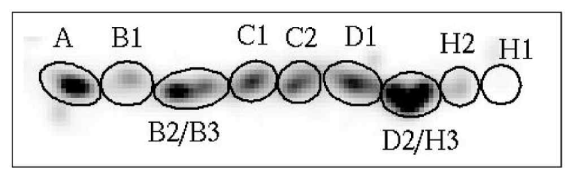
Figure 4.— Apertures used for radio and optical photometry, superposed on the HST jet image (same as Fig. 1b).

We also performed photometry at three radio wavelengths (VLA: 3.6, 2.0, and 1.3 cm) and three optical wavelengths (HST: $1.6\ \mu\rm m$, 620 nm, and 300 nm). The data sets used for the photometry are identical to those in Jester et al. (2005). We re-analyzed the photometric images because Jester et al. (2005) performed photometry with a $0\farcs 3$-aperture while we need knot-by-knot photometry to be directly compared with the infrared analysis. Unlike the infrared photometry described above, a PSF-fitting procedure is not mandatory since the knot separation of $\sim 1\arcsec$ is large compared to the spatial resolution. Therefore, defining regions as depicted in Fig. 4, we extracted the corresponding radio and optical fluxes inside each aperture region. The optical fluxes are corrected for Galactic extinction ($A_{V}=0.07$); correction factors used here are 1.01 for $1.6\ \mu\rm m$, 1.05 for 620 nm, and 1.12 for 300 nm, respectively. Photometric errors are small ($<5\%$) in all cases for both the radio and optical measurements. Possible systematic errors such as those associated with deconvolution in the interferometric radio data or flux contamination from adjacent knots, though difficult to quantify, would be several percents.

The morphologies of the knots in the jet are similar at all wavelengths; only the relative intensities of the knots change with frequency. The only exception to this is knot B1, in which the radio emission does not have a corresponding feature to the optical knot. This issue should be kept in mind when interpreting the spectrum of knot B1.

3.5. X-ray Photometry

Data used for the X-ray photometry presented here are based on four Chandra ACIS-S observations performed between November 2003 and July 2004 with Observation IDs (Obs IDs) from 4876 to 4879. The aimpoint was placed at the S3 CCD. The basic data reduction was done by using the CIAO software version 3.2.2 and the CALDB 3.1.0 with the standard screening criteria applied. Periods of background flaring often caused by the increased flux of charged particles in orbit have been excluded from each data set (e.g., a $\simeq 6\ \rm ks$ flare was found in the data of Obs ID 4879). After the screening processes a total exposure of 136 ks remains. We define three energy bands as 0.6–1 keV (soft), 1–2 keV (medium), and 3–6 keV (hard). The nominal energy $\varepsilon_{\rm norm}$ for each band is then the mean energy weighted by the effective area: $\varepsilon_{\rm norm}=$ 0.89 keV, 1.56 keV, and 4.35 keV, for the soft, medium, and hard band, respectively.

We have constructed X-ray flux images in the three bands with a pixel size of $0\farcs 2$ by dividing a counts map by an exposure map. These flux images, which are actually the weighted mean of four observation sets, have units of photons $\rm cm^{-2}\ s^{-1}\ keV^{-1}$ per pixel and allow us to perform X-ray photometry. Calculations of the exposure maps were performed with the CIAO tool mkexpmap assuming an incident spectrum of a power law with spectral index $\alpha=1$, correcting for the contamination buildup in the ACIS detectors. The results are insensitive to $\alpha$ since the corrections for different indices are minimal at the effective-area-weighted mean energy. Then we have measured the flux densities at $\varepsilon_{\rm norm}$ by integrating over relevant apertures and multiplying each image by $\varepsilon_{\rm norm}$. A similar but different procedure was adopted by Harris et al. (2004) to obtain the flux densities of the jet in 3C 120. Compared to the radio and optical cases (Fig. 4), we elongated the object apertures in the transverse $y$-direction ($|y|\leq 1\arcsec$) to accumulate photons such that the portion of photons lying outside the aperture should be $<10\%$. We estimated the background using regions outside the jet in the vicinity of the extraction apertures. The background amounts only to $\lesssim 2\%$ of the source flux for knot A even in the hard band where it has the largest contribution. Finally, to correct for the interstellar absorption of $N_{\rm H}=1.7\times 10^{20}\ \rm cm^{-2}$ (Albert et al., 1993), we multiplied the measured fluxes by a factor of 1.08 and 1.02 in the soft and medium energy bands, respectively. The flux densities of the knot regions determined in this way are given in Table 1. Most of the measurements have small statistical uncertainties less than 10%. The jet emission downstream of knot B2 does not show well discernible peaks but emission features associated with knots C1, D1, and D2/H3 can be recognized in the X-ray image, which justifies to some extent our aperture photometry for the downstream knots.

In addition to the photometry-based spectra, we have performed the more usual spectral analysis as a consistency check. The X-ray spectra in the 0.5–6 keV range of the four observations were simultaneously fitted by a power law with a fixed absorption column $N_{\rm H}=1.7\times 10^{20}\ \rm cm^{-2}$. The resultant spectral index for knot A is found to be $\alpha=0.84\pm 0.04$. Also, the index derived for a combined downstream region from knot C1 to D2/H3 is $\alpha=1.06\pm 0.07$. The photometry-based indices, on the other hand, are $\alpha\simeq 0.8$ and $\alpha\simeq 1.0$ for knot A and the combined downstream, respectively. Both methods are thus consistent with one another. It should be noted that we obtained somewhat steeper spectra, by $\Delta\alpha\sim 0.2$, compared to the results presented by Marshall et al. (2001). The difference arises most likely as a result of absorption by the molecular contaminants in the ACIS detectors. The presence of such contaminants was not known at the time of the Marshall et al. (2001) analysis and consequently their spectral analyses inevitably led to a systematically lower $\alpha$. Similarly, Perlman & Wilson (2005) reanalyzed early Chandra data on the M 87 jet and found that contamination of the ACIS detector can account for the flatter X-ray spectra than expected based on the optical slope as reported by Wilson & Yang (2002, see their erratum).

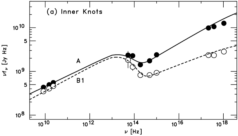
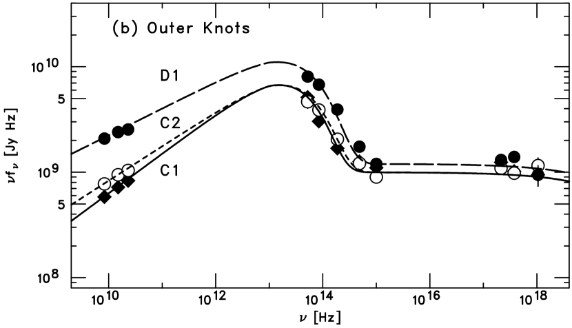
Figure 5.— Broadband SEDs of the 3C 273 large-cale jet. (a) Inner knots A (filled circles) and B1 (open circles); (b) outer knots C1 (diamonds), C2 (open circles), and D1 (filled circles). The photometric data are given in Table 1. The curves represent the two-component phenomenological model, namely equation (1): $f_{\nu}=\kappa_{1}\nu^{-\alpha_{1}}\exp\left[-\left(\nu/\nu_{c}\right)^{a}\right]+\kappa_{2}\nu^{-\alpha_{2}}$ with parameters in Table 2. Note that $1\ \rm Jy\,Hz=10^{-23}\ erg\ cm^{-2}\ s^{-1}$. Figure 6 zooms in the mid-infrared to ultraviolet part, where the photometric points are relatively cramped.

4. Results and Discussion

4.1. SED of Jet Knots: Two-Component Nature

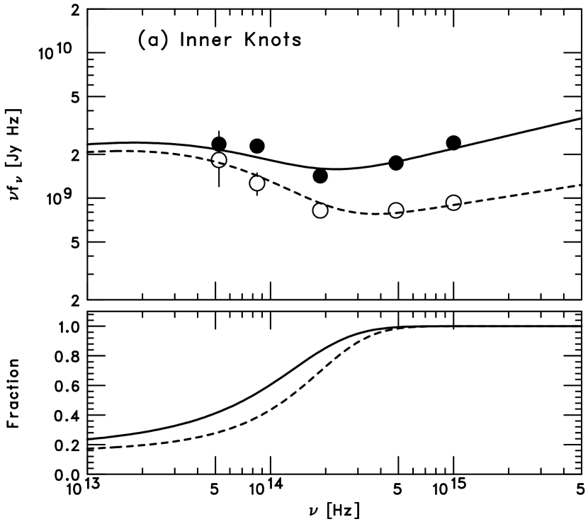
Figure 6.— (Top) Close-up views (with same symbols) of the SEDs shown in Fig. 5 for the infrared-to-optical range. (Bottom) The contribution of the high-energy component relative to the total emission in terms of the two-component phenomenological model.

In Fig. 5, we show the SEDs constructed for knots A, B1, C1, C2, and D1. Since the interpretation of multiple knots (B2/B3 and D2/H3) could be misleading, the “summed” spectra for B2/B3 and D2/H3 have been omitted in Fig. 5 and in the spectral modeling described below. The overall spectral appearance of the inner knots (A and B1) has strikingly different characteristics as compared to the outer knots (C1, C2, and D1). First, the inner knots radiate strongly in the X-ray (or even beyond) with hard spectra while the outer knots radiate predominantly in the mid-infrared. Second, and most importantly, the SEDs of the inner knots have a concave shape from the mid-infrared to optical band, indicating that two spectral components cross over at optical wavelengths. Figure 6 gives a close-up version of Fig. 5 highlighting the mid-infrared to near-ultraviolet part of the spectrum. We emphasize here that the IRAC fluxes fill a critical region in the SEDs, making it possible to identify unambiguously the spectral structures present in the infrared to optical wavelengths.

In the SEDs of the inner knots, we identify two spectral components, namely (1) the low-energy synchrotron spectrum extending from radio to infrared with a spectral cutoff at $\sim 5\times 10^{13}$ Hz, and (2) the high-energy component arising in the optical and smoothly connecting to the X-ray flux. Tentatively, we suggest that the high-energy component is likely of synchrotron origin, because the optical polarization is consistent with the radio polarization in degree and orientation. In §§4.3 and 4.4 we discuss the origin of the high-energy spectral component and its implications to particle acceleration in the jet. In explaining the broadband spectrum of knot A, a single power-law continuum all the way from radio to X-ray has been proposed in prior studies (Röser et al., 2000; Marshall et al., 2001), but this picture does not correctly describe the present, more extensive data.

In the outer knots, the SEDs also show the two components but with different relative strengths. The low-energy part becomes more dominant with increasing distance from the quasar core. At first glance the entire infrared-optical spectrum may be attributed to the falling part of synchrotron emission. However, careful inspection shows a slight spectral-flattening in the optical and near-ultraviolet, which suggests a contribution from the second component responsible for the X-ray emission, as already proposed by Jester et al. (2002). This idea is further strengthened by the observation that the radio brightening in D1 (relative to C1/C2) accompanies infrared brightening while the near-ultraviolet and X-ray fluxes remain at similar levels (see Fig. 6).

To visualize the spectral transition from the inner to the outer knots along the jet, we present a three-color image of the jet in Fig. 7 based on the data taken with Spitzer, HST, and Chandra, with the VLA contours from Fig. 1 overlaid. The colors are coded as follows: Spitzer $3.6\ \mu\rm m$ (red), HST $f_{0.3\mu\rm m}-0.05\times f_{1.6\mu\rm m}$ (green), Chandra 0.4–6 keV (blue). The Spitzer image is a “deconvolved” IRAC image, which represents the results of our infrared photometry via PSF-fitting in §3.3. Specifically, the best-fit image obtained with two-dimensional fitting is artificially shrunk to match the effective resolution of the HST image. The HST image is an “UV excess” map [determined as $f_{0.3\mu\rm m}-0.05\times f_{1.6\mu\rm m}$ based on the data in Jester et al. (2005)] representing the dominance of near-ultraviolet light over the near-infrared. It is clear that the inner knots are luminous in both the UV excess and X-rays (the high-energy component), while the outer knots are bright in the mid-infrared (the low-energy component).

Table 2Phenomenological Model Parameters of 3C 273 Jet Knots

Parameter	A	B1	C1	C2	D1	H2	H1
$\alpha_{1}$	0.76	0.73	0.63	0.68	0.75	0.9	0.9
$\nu_{c}$ (Hz)	$5\times 10^{13}$	$5\times 10^{13}$	$4\times 10^{13}$	$5\times 10^{13}$	$6\times 10^{13}$	$5\times 10^{13}$	$4\times 10^{13}$
$a$	0.8	0.8	0.8	0.8	0.8	0.8	0.8
$\alpha_{2}$	0.7	0.8	1.0	1.0	1.0	$\cdots$	$\cdots$

We describe the radio-to-X-ray spectra with the following double power-law models (one with an exponential cutoff):

$$f_{\nu}=f_{1\nu}+f_{2\nu}=\kappa_{1}\nu^{-\alpha_{1}}\exp\left[-\left(\nu/\nu_{c}\right)^{a}\right]+\kappa_{2}\nu^{-\alpha_{2}}.$$ (1)

The first term of the right-hand-side accounts for the low-energy spectrum and the second pure power-law describes the high-energy part. (For the second component, $f_{2\nu}=\kappa_{2}\nu^{-\alpha_{2}}$, we set an artificial low-energy turn-over below $10^{13}$ Hz.) We introduced a parameter $a$ in the exponential part because particle acceleration models generally do not provide a robust prediction concerning the electron spectrum in the cutoff region. We adopt a common value of $a=0.8$; the choice has little influence on other parameters. Table 2 lists the spectral parameters that well describe the knot SEDs shown in Fig. 5. Also, in Fig. 6 we show the relative contribution of the second component, namely $f_{2\nu}/(f_{1\nu}+f_{2\nu})$, in the infrared to ultraviolet part. It should be noted that the second component is dominant ($>80\%$) already in the $R$ band flux and therefore the “optical” jet traces the high-energy radiation. For knot A, the first component has a luminosity of $1.3\times 10^{43}\ \rm erg\ s^{-1}$ (in the frequency range $10^{9}\mbox{--}10^{14}$ Hz) without taking account of relativistic beaming. The minimum luminosity in the second component of knot A is $3.4\times 10^{43}\ \rm erg\ s^{-1}$ ($10^{14}\mbox{--}10^{18}$ Hz), and can be much higher if the spectrum extends well beyond the X-ray domain.

The spectral index of the low-energy component is in the range of $\alpha_{1}=0.63\mbox{--}0.76$, as determined from the radio spectra. Remarkably, the cutoff frequency is quite similar among the knots, $\nu_{c}=(4\mbox{--}6)\times 10^{13}$ Hz, which differs from previous modeling that deduced a progressive decrease of the cutoff frequencies (see Jester et al., 2005, and references therein). The difference in the deduced cutoff frequency results from our inclusion of the IRAC fluxes into the modeling. The second spectral index for knots A and B1 is $\alpha_{2}=0.7\mbox{--}0.8$; for knots C1, C2 and D1, the second index is steeper, $\alpha_{2}\simeq 1.0$. It should be emphasized that the second index of knot A agrees well with the local spectral index determined by X-rays alone, in other words $\alpha_{2}\simeq\alpha_{\rm x}$. Interestingly, the steepness of the index seems to increase with decreasing X-ray intensity of the knots.

There are some caveats for the interpretation of the SEDs that we constructed. As mentioned earlier, knot B1 in the optical shows a different morphology as compared to the radio one. Therefore, the first and second components should originate in different emission volumes. Also, the X-ray flux assigned for knot B1 could be contaminated by adjacent, bright knots.

Figure 7.— Spitzer-HST-Chandra composite image of the jet of 3C 273. The colors are coded as follows: Spitzer “deconvolved” $3.6\ \mu\rm m$ (red), HST “UV excess” $f_{0.3\mu\rm m}-0.05\times f_{1.6\mu\rm m}$ (green), Chandra 0.4–6 keV (blue). The VLA radio (2 cm) contours are superposed on the image, with the strongest radio source H2 being truncated. There are two distinct types of radiating knots; the inner knots show hard optical spectra (green) and strong X-rays (blue) while the outer knots show bright infrared (red).

4.2. Physical Parameters for the Low-Energy Component

The cutoff frequency of the low-energy synchrotron emission that we determined in the previous section represents the maximum energy of the associated electron population. According to standard synchrotron theory (e.g., Ginzburg & Syrovatskii, 1965), the maximum energy can be estimated as

$$E_{\max}\simeq 0.28\ \left[\frac{1+z}{\delta}\right]^{0.5}\left(\frac{B}{0.1\ \rm mG}\right)^{-0.5}\left(\frac{\nu_{\rm c}}{10^{14}\ \rm Hz}\right)^{0.5}\ \rm TeV,$$ (2)

where $\delta$ is the Doppler factor, $z=0.158$ is the redshift, and $B$ is the comoving magnetic field strength. The Doppler factor is defined as $\delta\equiv[\Gamma(1-\beta\cos\theta)]^{-1}$ with $\beta c$ the velocity of the jet, $\Gamma=(1-\beta^{2})^{-1/2}$ the bulk Lorentz factor of the jet, and $\theta$ the observing angle with respect to the jet direction. It is difficult to determine the Doppler factor, and therefore to what extent the observed jet radiation is enhanced by Doppler beaming. Furthermore, the jet may be decelerating along the observed jet portion resulting in a declining Doppler factor (Georganopoulos & Kazanas, 2004; Tavecchio et al., 2006). A likely range is $1<\delta<10$ (see however §4.4). If equipartition between the radiating electrons and magnetic fields is assumed, without taking into account any relativistic motion (i.e., $\delta=1$), one can obtain an estimate of $B=0.1\mbox{--}0.2\ \rm mG$ (Jester et al., 2005). Therefore, given the cutoff frequencies of $\nu_{c}\simeq 5\times 10^{13}$ Hz, the maximum energy can be deduced as $E_{\rm max}\sim 0.2\ (B_{-4}\delta)^{-0.5}\ \rm TeV$, where $B_{-4}=B/(0.1\ \rm mG)$. According to the prescription given in Harris & Krawczynski (2002), the equipartition condition yields $B\propto\delta^{-1}$ (see, Stawarz et al., 2003, for slightly different scaling). Then, an estimate of $E_{\rm max}$ is rather robust being nearly independent of both $\delta$ and $B$.

Synchrotron cooling in the source should affect the spectral shape provided that the cooling time is shorter than the formation timescale of the radiating knots. The synchrotron cooling time (in the jet comoving frame) for electrons with energy $E=\gamma m_{e}c^{2}$ emitting on average at a frequency $\nu$ (observed) can be expressed as

$$t_{\rm syn} = \frac{\gamma m_{e}c^{2}}{(4/3)c\sigma_{\rm T}U_{B}\gamma^{2}},$$ (3)

$$\simeq 2400\,\left[\frac{\delta}{1+z}\right]^{0.5}\left(\frac{B}{0.1\ \rm mG}\right)^{-1.5}\left(\frac{\nu}{10^{14}\ \rm Hz}\right)^{-0.5}\rm yr,$$ (4)

where $\sigma_{\rm T}$ is the Thomson cross section, and $U_{B}=B^{2}/(8\pi)$ is the energy density of the magnetic field. Equation (2) was used in relating $E=\gamma m_{e}c^{2}$ with $\nu$, by replacing $E_{\max}$ with $E$ and $\nu_{\rm c}$ with $(\nu/0.29)$. The source age, though quite uncertain, would be $t_{0}\sim 10^{5}\mbox{--}10^{7}\ \rm yr$. Therefore, the observed synchrotron spectra from the radio to optical frequencies are likely to be formed in the “cooling regime”, namely $t_{\rm syn}<t_{0}$, which means that a continuous injection of electrons with an acceleration spectrum of $Q(E)\propto E^{-s_{1}}$ (in the power-law part) over the timescale $t_{0}$ gives rise to the energy distribution of synchrotron-emitting electrons $N(E)\propto t_{\rm syn}Q(E)\propto E^{-(s_{1}+1)}$. In this case, according to the relation $s_{1}=2\alpha_{1}$, the observed index of $\alpha_{1}\simeq 0.7$ is translated into the electron acceleration index of $s_{1}\simeq 1.4$, which is coincident with the hardest possible index ($s=1.5$) in the nonlinear shock acceleration theory (Malkov & Drury, 2001). We implicitly assumed particle acceleration taking place in each knot (Jester et al., 2001), where relativistic electrons are accumulated without escaping. A similar treatment was applied to the hotspot of 3C 273 by Meisenheimer & Heavens (1986) to incorporate a shock-acceleration theory into the emerging radiation spectrum. There may be occasions for which the above argument is not applicable; for example, in the case of significant beaming, the synchrotron cooling time would be much longer ($t_{\rm syn}\propto\delta^{2}$ for the equipartition field) and the realization of the cooling regime would not be justified for radio-emitting electrons.

4.3. Synchrotron Interpretation of the High-Energy Component

For the inner knots (A and B) we have found that the optical and X-ray fluxes can be modeled as a common power-law spectrum of spectral index $\alpha_{2}\simeq 0.7\mbox{--}0.8$. Also, the optical to X-ray slope agrees with the X-ray spectral index, especially for knot A, $\alpha_{2}\simeq\alpha_{\rm x}$. One implication of this finding is that the optical and X-ray fluxes must be explained by the same emission mechanism. In §2 we mentioned that both the radio and optical jet emission are linearly polarized to a similar degree of $\sim 15\%$ (Röser & Meisenheimer, 1991; Röser et al., 1996), which has been taken as evidence for a synchrotron origin for the optical radiation in the inner knots. Now this in turn would imply a synchrotron origin for the X-ray radiation as well. Therefore we first discuss the optical-X-ray component in terms of synchrotron radiation produced by high-energy electrons.

According to the prescription in §4.2, the power-law slope of the energy distribution of the accelerated electrons is $s_{2}=2\alpha_{2}$ in the synchrotron-cooling regime. Then the spectral index of the high-energy component, $\alpha_{2}\simeq 0.7\mbox{--}0.8$ for the inner knots, yields $s_{2}\simeq 1.4\mbox{--}1.6$. Interestingly, the index of acceleration is almost same between the low- and high-energy synchrotron components: $s_{2}\sim s_{1}$ (because of $\alpha_{2}\sim\alpha_{1}$). On the other hand, the two indices differ in the outer knots: $\alpha_{2}\simeq 1$, corresponds to $s_{2}\simeq 2$.

The apparent difference in the cutoff frequency between the low- and high-energy components likely reflects a difference in the maximum energy of electron acceleration. The cutoff frequency associated with the high-energy component is not constrained by the current data, but must be greater than $10^{18}$ Hz ($\sim 4$ keV). Consequently, from equation (2), the lower limit to the maximum electron energy is $E_{\rm max}\gtrsim 30\ (B_{-4}\delta)^{-0.5}\ \rm TeV$.

The presence of two different cutoff energies suggests two acceleration modes that can be characterized by different acceleration rates in the knots. The acceleration timescale can be expressed as $t_{\rm acc}=\xi r_{g}/c$, with a gyroradius $r_{g}=E/(eB)$. The rate of acceleration is parametrized by the factor $\xi\geq 1$ which is, as frequently assumed, taken to be energy independent. By equating $t_{\rm acc}=t_{\rm syn}$—namely, balancing the acceleration and synchrotron loss rates—one obtains the maximum attainable energy limited by synchrotron losses:

$$E_{\max}\simeq 6\times 10^{15}\ \xi^{-0.5}\left(\frac{B}{0.1\ \rm mG}\right)^{-0.5}\ \rm eV.$$ (5)

Using equation (2) this can be translated into the corresponding cutoff frequency,

$$\nu_{\rm c}\simeq 4.5\times 10^{22}\ \xi^{-1}\frac{\delta}{1+z}\ \rm Hz.$$ (6)

Therefore, for the second synchrotron component to extend beyond $10^{18}$ Hz, the condition $\xi_{2}<4\times 10^{4}$ should be fulfilled. On the other hand, for the low-energy synchrotron component, an extremely large value of $\xi_{1}\sim 10^{9}$ can be inferred via a similar argument. Interestingly, a study of multiwavelength spectra of small-scale blazar emission also gives large $\xi$ (Inoue & Takahara, 1996).

In the theory of diffusive shock acceleration, for relativistic shocks, the factor $\xi$ corresponds roughly to the ratio of the energy density of regular magnetic fields to that of turbulent fields which resonantly scatter accelerating relativistic particles. Then a different value of $\xi$ means a different development of turbulent magnetic fields near the shock. The inferred large value of $\xi_{1}$, following a discussion in Biermann & Strittmatter (1987), may be understood in terms of steep turbulence spectra, e.g., of Kolmogorov-type $I(k)\propto k^{-5/3}$ [where $I(k)$ is the magnetic energy density per wavenumber $k$ in the turbulent field], though it should be noted that $I(k)\propto k^{-1}$ was silently assumed above to obtain energy-independent $\xi$ for simplicity.

There may be two distinct types of shocks characterized by different $\xi$ in the knots giving rise to their “double-synchrotron” nature. Alternatively, another acceleration mechanism may be operating, accounting in a natural way for a different acceleration rate for the second component. For instance, turbulent acceleration may occur in the shear of jet boundary layers (Ostrowski, 2000), generating the second synchrotron component (Stawarz & Ostrowski, 2002). In highly turbulent shear layers, the acceleration rate can be estimated as $\xi\sim\beta_{\rm A}^{-2}$, where $\beta_{\rm A}$ denotes the Alfvèn velocity in units of $c$. Provided that the jet is composed of electron-proton plasma with the comoving number density $n$ (Sikora & Madejski, 2000), the Alfvèn velocity in the jet can be written as

$$\beta_{\rm A} = \frac{B}{\sqrt{4\pi nm_{\rm p}}}$$ (7)

$$= 7.3\times 10^{-2}\left(\frac{B}{0.1\ \rm mG}\right)\left(\frac{n}{10^{-4}\ \rm cm^{-3}}\right)^{-0.5}.$$ (8)

The condition $\xi_{2}<4\times 10^{4}$ needed to produce the X-rays can be fulfilled if $\beta_{\rm A}>5\times 10^{-3}$, which seems reasonable for the typical jet parameters.

An intriguing implication of interpreting the X-ray emission as being due to a synchrotron process would be the possibility that protons in the jet can be accelerated to very high energies. In the case of protons, synchrotron losses do not limit the acceleration process unless they reach ultra-high energies. Instead, a condition set by $t_{\rm acc}=t_{\rm c}$, where $t_{\rm c}$ is the light-crossing timescale of the knot along the jet (typically $\sim 10$ kyr), would give a conservative estimate of the maximum attainable energy of protons. Here we use a light-crossing time rather than the “age” of the jet, probably $t_{0}\sim 10^{5}\mbox{--}10^{7}\ \rm yr$, to conservatively account for an escape loss which takes at least longer than a light-crossing time. This condition leads to

$$E_{\rm p,max} = \xi^{-1}ecBt_{\rm c}$$ (9)

$$\simeq 2.8\times 10^{20}\ \xi^{-1}\left(\frac{B}{0.1\ \rm mG}\right)\left(\frac{t_{\rm c}}{10\ \rm kyr}\right)\ \rm eV,$$ (10)

and consequently $E_{\rm p,max}>0.7\times 10^{16}\ \rm eV$ for $\xi<4\times 10^{4}$ and typical values of $B$ and $t_{\rm c}$. Remarkably, if $\xi\sim 10$ (close to the so-called Bohm diffusion in the framework of diffusive shock acceleration), ultra-high-energy protons with energies $E_{\rm p,max}\sim 10^{19}\ \rm eV$ can be accelerated in the jet of 3C 273 (see Aharonian, 2002; Honda & Honda, 2004, for detailed theoretical arguments). Even with a large value of $\xi$ ($\gtrsim 100$), the shear acceleration would still be capable of generating $E_{\rm p,max}\sim 10^{19}\ \rm eV$, since the turbulent acceleration in the shear layer may be available for much longer timscales. The fraction of jet power that goes to high energy protons depends on the particle content of the jet and the details of the physics of particle acceleration, both of which are not well known.

It is interesting to note that if protons are indeed accelerated in the jet to very high energies, $E_{\rm p,max}\gtrsim 10^{18}\ \rm eV$, the second synchrotron component can be produced directly by protons, i.e., proton synchrotron radiation (Aharonian, 2002), rather than by electrons. For the same particle energy, the characteristic frequency of proton synchrotron radiation, $\nu_{\rm p,c}$, is less than that of electron synchrotron radiation by a factor of $(m_{\rm e}/m_{\rm p})^{3}$. Therefore, by using equation (2), the spectrum of proton synchrotron has a cutoff frequency of

$$\nu_{\rm p,c}\simeq 2.1\times 10^{18}\ \left[\frac{\delta}{1+z}\right]\left(\frac{B}{\rm mG}\right)\left(\frac{E_{\rm p,max}}{10^{18}\ \rm eV}\right)^{2}\ \rm Hz,$$ (11)

which is located above the X-ray domain. Thus protons rather than a second population of electrons, may explain the second synchrotron component. Unlike the electron-synchrotron case, the diffuse nature of the emission (at least in the optical) can be understood more easily thanks to much longer cooling timescale for protons. A magnetic field strength of $\gtrsim 1\ \rm mG$ is needed in order to keep the power spent to accelerate protons at a reasonable level, and at the same time to render the acceleration timescale shorter and the diffusion timescale longer (Aharonian, 2002). By adopting $B=10\ \rm mG$, $\delta=1$, an escape loss timescale of $t_{\rm esc}=1.4\times 10^{7}(E_{\rm p}/10^{14}\ \rm eV)^{-1/2}\ yr$, and a continuous proton injection over $t_{0}=3\times 10^{7}\ \rm yr$, Aharonian (2002) obtained the acceleration power for protons of $L_{\rm p}\simeq 10^{46}\ \rm erg\ s^{-1}$ to explain the optical-X-ray spectrum of knot A in 3C 273 in terms of proton synchrotron radiation.

4.4. Beamed IC Model for the High-Energy Component

Previous explanations of the second, X-ray-dominated component of the SED for jet knots have emphasized the beamed IC scenario (Tavecchio et al., 2000; Celotti et al., 2001). Specifically, relativistically beamed IC emission in the CMB photon field has been invoked to model the X-ray emission in 3C 273 (Sambruna et al., 2001), as well as in other quasar jets. This model requires a highly relativistic bulk velocity of the jet, with a Doppler factor $\delta\sim 10$ out to nearly megaparsec distances. A direct connection between the optical and X-ray fluxes in the inner knots A and B1 and also between the ultraviolet and X-ray fluxes in the outer knots (see Fig. 5) led us to consider that the same mechanism should be responsible for the optical and X-ray emissions, forming a distinct high-energy component. If one adopts the beamed IC model for the X-rays, the optical fluxes in the inner knots and the ultraviolet fluxes in the outer knots should be explained also by the beamed IC radiation. This implies that the energy distribution of electrons has to continue down to very low energies of $E_{\rm min}\sim m_{e}c^{2}$ without a cutoff or break.

In this scenario, one still should account for the optical polarization. In the case of “cold” electrons in the jet, Compton up-scattering off the CMB by an ultrarelativistic jet (so-called “bulk Comptonization”) can yield in principle a high degree of polarization for the standard choice of $\theta\simeq\Gamma^{-1}$ (Begelman & Sikora, 1987). However, for relativistic electrons with $E\sim 2\,m_{e}c^{2}$ as appropriate for the optical IC emission in this jet, the degree of polarization should be significantly reduced (Poutanen, 1994). The present data of the radio and optical polarization (Röser et al., 1996) may require a tuned set of physical conditions to reconcile with the beamed IC scenario.

In this respect, a possible caveat would be that in addition to the CMB, the synchrotron radiation of the jet itself might serve as seed photons for Compton up-scattering; if the highly relativistic jet accompanies slowly moving outer portions, the synchrotron radiation that comes from the slowing part can be relativistically enhanced in the fast moving jet, providing the effective photon fields for Comptonization (Ghisellini, Tavecchio & Chiaberge, 2005, as discussed for small-scale jets). If the observed radio flux is largely contributed by a slow, non-relativistic layer, the energy density of the synchrotron photons (as measured in the observer’s frame) could reach $\sim 10^{-12}\ \rm erg\ cm^{-3}$, being comparable to the CMB energy density. This possibility introduces a complication to the polarization argument.

Within the framework of the beamed IC radiation, the physical parameters that can reproduce the SEDs of the 3C 273 jet have been obtained (e.g., Sambruna et al., 2001; Harris & Krawczynski, 2002). Compared to a typical value of $E_{\rm min}\sim 20\,m_{e}c^{2}$ in the previous work (e.g., Sambruna et al., 2001), a smaller minimum energy of the electron distributions, say $E_{\rm min}\sim m_{e}c^{2}$, is required by the present data. Note that this increases the estimate of the jet kinetic power by an order of magnitude if the jet power is dynamically dominated by cold protons. Let us model the SED of knot A with a synchrotron plus beamed IC model of Tavecchio et al. (2000) assuming $\delta=\Gamma$ and a knot radius of 1 kpc (in the jet frame of reference). For a Doppler factor of $\delta=30$ and magnetic field $B=5\ \mu$G as roughly corresponding to an equipartition condition, we obtain a jet kinetic power of $L_{\rm jet}\simeq 1\times 10^{48}\ \rm erg\ s^{-1}$, if the number of the observed electrons is balanced by the number of cold protons in the jet. However, such a large Doppler factor of $\delta=30$ seems problematic, since relatively large contributions from the un-beamed components are observed in the core emission, such as an ultraviolet bump (see Courvoisier, 1998, and references therein), and the accretion-disk emission comparable to the jet emission in the X-ray regime (Grandi & Palumbo, 2004). Instead, if we adopt a smaller Doppler factor of $\delta=10$ (together with $E_{\rm min}=3\,m_{e}c^{2}$ to account for the optical emission), the energy density of electrons exceeds that of magnetic fields more than three orders of magnitude, and the jet kinetic power reaches an uncomfortable level of $L_{\rm jet}\simeq 1\times 10^{49}\ \rm erg\ s^{-1}$. To summarize, the beamed IC model, in its simple form, does not easily find a satisfactory set of parameters, particularly for the case of knot A.

Finally, the upper limit to the infrared fluxes from the quiet portion of the jet upstream of knot A is important to constrain the structure of the jet in the context of the beamed IC model (Georganopoulos et al., 2005; Uchiyama et al., 2005). Unfortunately, we need additional IRAC observations to derive a reliable upper limit there because of the large systematic uncertainty in PSF subtraction in the region close to the quasar core.

4.5. The Head Region

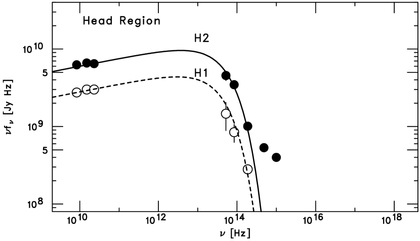
Figure 8.— Broadband SEDs of the head region of the 3C 273 jet: H2 (filled circles) and H1 (open circles). The photometric data are given in Table 1. The curves represent the single-component model (see the text).

In Fig. 8, we show the SEDs obtained for H1 and H2 in the head region. Note that no significant X-ray emission was found in this region. We have modeled the SEDs using a power law with an exponential-type cutoff, namely by equation (1) with $\kappa_{2}=0$, as drawn in Fig. 8. The spectral parameters used for the model are indicated in Table 2. Interestingly, the spectrum of H2 shows a notable flattening at the optical and ultraviolet wavelengths, as first reported by Jester et al. (2005).

The radio spectra are steeper than those of the upstream knots, with $\alpha\simeq 0.9$. It is likely that particle acceleration acting in the head region would be terminal shocks that have different properties as compared to upstream shocks. As argued by Meisenheimer & Heavens (1986), if the effect of synchrotron cooling is taken into account, the index seems consistent with an acceleration spectrum of $Q\propto E^{-2}$, which is the standard spectrum of diffusive shock acceleration. Within the picture proposed by Meisenheimer & Heavens (1986), however, the excess fluxes at optical and ultraviolet wavelengths seen in the spectrum of H2 cannot be easily understood. These excesses may represent a second synchrotron component just as in the case of the upstream knots.

5. Conclusions

We have presented results from our Spitzer IRAC observation of the 3C 273 jet at wavelengths 3.6 and $5.8\ \mu\rm m$, combined with the photometry with the VLA radio, HST optical, and Chandra X-ray data. Our multiwavelength analysis led us to conclude that the flat optical emission in the X-ray-dominated knots originates in the high-energy power-law component, which also accounts for the X-ray emission. The agreement between the optical-X-ray slope ($\alpha_{2}$) and the X-ray spectral index ($\alpha_{\rm x}$) throughout the jet supports this picture. On the other hand, the radio to infrared spectra can be expressed by a power law with an exponential cutoff at $\sim 5\times 10^{13}$ Hz. The two distinct radiation components, namely low-energy (radio-infrared) and high-energy (optical-X-ray) emission, have similar power of $\sim 10^{44}\ \rm erg\ s^{-1}$ for the entire jet volume (without a beaming correction); the power in the second component becomes noticeably higher if its peak position is located far beyond the X-ray domain. The relative importance of the two components changes along the jet (see Fig. 7). In the inner, X-ray-dominated knots, the high-energy component overwhelms the low-energy one.

The second component can be attributed to either synchrotron radiation by a second population of high-energy electrons (or protons), or the beamed IC emission by the radio-emitting electrons. In the first case, the double synchrotron nature may arise from the presence of distinctively different acceleration processes (e.g., shock and turbulent acceleration). In the context of the origin of extragalactic cosmic-rays, it is interesting that a faster acceleration mechanism producing the second component is capable of accelerating cosmic-ray protons to energies $10^{16}\ \rm eV\lesssim E_{\rm p,max}\lesssim 10^{19}\ \rm eV$. On the Comptonization interpretation of the high-energy emission, we argued that the present polarization data seems problematic. Future sensitive measurements of polarization are quite important to draw firmer conclusions about the origin of the high-energy emission.

The identification of the synchrotron component peaking at $\sim 5\times 10^{13}\ \rm Hz$ in the X-ray-dominated knots of the 3C 273 jets calls for a follow-up deep observation with the Spitzer IRAC with better configurations. Our Spitzer cycle-3 proposal (PI: Uchiyama) requesting follow-up deep observations of 3C 273, as well as the observations of 10 other jets, has recently been approved. Ultimately, the James Webb Space Telescope, a future large infrared-optimized space telescope, will have an excellent capability to explore the jet emission in the IRAC band with much improved resolution and sensitivity.

An interesting implication of this work is that a number of optical jets in radio-loud quasars discovered so far may be directly related to the X-ray emission rather than to the radio emission, as in the 3C 273 jet. For example, in Uchiyama et al. (2005), we have associated the optical flux of the jet knot in the quasar PKS 0637$-$752 with the highest energy part of the synchrotron component. However, the optical flux could be attributed equally to the low energy part of the second component, given the result presented here. This issue should be addressed in future analyses based on multiwavelength observations of Chandra-detected quasar jets. [In this context, we note that our discussions are not concerned with low-luminosity FR I jets such as M 87 (e.g., Perlman & Wilson, 2005), in which the X-ray emission appears to lie on the extrapolation of the emission at lower frequencies, and is widely believed to be of synchrotron origin.] It is clear from our results that the measurements over as wide a wavelength coverage as possible in the infrared-optical domain are of great importance in studying the particle acceleration mechanisms in the large-scale jets of powerful quasars. Unfortunately, quasar jet emission in the optical region of the spectrum is very faint, and only a few optical slopes for the powerful quasars have been measured (Ridgway & Stockton, 1997; Cheung, 2002). Further Spitzer observations are therefore particularly helpful even though the spatial resolution is not optimal for the study of jet emissions. Also, a careful measurement of X-ray spectral index and its comparison with the optical fluxes is valuable to progress toward the understanding of the dominant X-ray emission mechanism operating in the quasar jets.

References

- Aharonian (2002) Aharonian, F. A. 2002, MNRAS, 332, 215
- Albert et al. (1993) Albert, C. E., Blades, J. C., Morton, D. C., Lockman, F. J., Proulx, M., & Ferrarese, L. 1993, ApJS, 88, 81
- Atoyan & Dermer (2001) Atoyan, A. M., & Dermer, C. D. 2001, Phys. Rev. Lett., 87, 221102
- Atoyan & Dermer (2003) Atoyan, A. M., & Dermer, C. D. 2003, ApJ, 586, 79
- Atoyan & Dermer (2004) Atoyan, A. M., & Dermer, C. D. 2004, ApJ, 613, 151
- Bahcall et al. (1995) Bahcall, J. N., Kirhakos, S., Schneider, D. P., Davis, R. J., Muxlow, T. W. B., Garrington, S. T., Conway, R. G., & Unwin, S. C. 1995, ApJ, 452, L91
- Begelman & Sikora (1987) Begelman, M. C., & Sikora, M. 1987, ApJ, 322, 650
- Biermann & Strittmatter (1987) Biermann, P. L., & Strittmatter, P. A. 1987, ApJ, 322, 643
- Celotti et al. (2001) Celotti, A., Ghisellini, G., & Chiaberge, M. 2001, MNRAS, 321, L1
- Chartas et al. (2000) Chartas, G., et al. 2000, ApJ, 542, 655
- Cheung (2002) Cheung, C. C. 2002, ApJ, 581, L15
- Conway et al. (1993) Conway, R. G., Garrington, S. T., Perley, R. A., & Biretta, J. A. 1993, A&A, 267, 347
- Courvoisier (1998) Courvoisier, T. J. -L. 1998, A&A Rev., 9, 1
- Dermer & Atoyan (2002) Dermer, C. D., & Atoyan, A. M. 2002, ApJ, 568, L81
- Davis et al. (1985) Davis, R. J., Muxlox, T. W. B., & Conway, R. G. 1985, Nature, 318, 343
- Fazio et al. (2004) Fazio, G., et al. 2004, ApJS, 154, 10
- Fruchter & Hook (2002) Fruchter, A. S., & Hook, R. N. 2002, PASP, 114, 144
- Georganopoulos & Kazanas (2004) Georganopoulos, M., & Kazanas, D. 2004, ApJ, 604, L81
- Georganopoulos et al. (2005) Georganopoulos, M., Kazanas, D., Perlman, E., & Stecker, F. W. 2005, ApJ, 625, 656
- Ghisellini, Tavecchio & Chiaberge (2005) Ghisellini, G., Tavecchio, F., & Chiaberge, M. 2005, A&A, 432, 401
- Ginzburg & Syrovatskii (1965) Ginzburg, V. L., & Syrovatskii, S. I. 1965, ARA&A, 3, 297
- Grandi & Palumbo (2004) Grandi, P., & Palumbo, G. G. C. 2004, Science, 306, 998
- Hao et al. (2005) Hao, L., et al. 2005, ApJ, 625, L75
- Hardcastle (2006) Hardcastle, M. 2006, MNRAS, 366, 1465
- Harris & Krawczynski (2002) Harris, D. E., & Krawczynski, H. 2002, ApJ, 565, 244
- Harris et al. (2004) Harris, D. E., Mossman, A. E., & Walker, R. C. 2004, ApJ, 615, 161
- Harris & Stern (1987) Harris, D. E., & Stern, C. P. 1987, ApJ, 313, 136
- Honda & Honda (2004) Honda, Y. S., & Honda, M. 2004, ApJ, 613, L25
- Inoue & Takahara (1996) Inoue, S., & Takahara, F. 1996, ApJ, 463, 555
- Jester et al. (2002) Jester, S., Röser, H.-J., Meisenheimer, K., & Perley, R. A. 2002, A&A, 385, L27
- Jester et al. (2005) Jester, S., Röser, H.-J., Meisenheimer, K., & Perley, R. A. 2005, A&A, 431, 477
- Jester et al. (2001) Jester, S., Röser, H.-J., Meisenheimer, K., Perley, R. A., & Conway, R. G. 2001, A&A, 373, 447
- Kataoka & Stawarz (2005) Kataoka, J., & Stawarz, Ł. 2005, ApJ, 622, 797
- Makovoz & Marleau (2005) Makovoz, D., & Marleau, F. R. 2005, PASP, 117, 1113
- Malkov & Drury (2001) Malkov, M. A., & Drury, L. O’C. 2001, Rep. Prog. Phys., 64, 429
- Marshall et al. (2001) Marshall, H. L., et al. 2001, ApJ, 549, L167
- Marshall et al. (2005) Marshall, H. L., et al. 2005, ApJS, 156, 13
- Martel et al. (2003) Martel, A. R., et al. 2003, AJ, 125, 2964
- McLeod & Rieke (1994) McLeod, K. K., & Rieke, G. H. 1994, ApJ, 431, 137
- Meisenheimer & Heavens (1986) Meisenheimer, K., & Heavens, A. F. 1986, Nature, 323, 419
- Neronov et al. (2002) Neronov, A., Semikoz, D., Aharonian, F., Kalashev, O. 2002, Phys. Rev. Lett., 89, 051101-1
- Neumann et al. (1997) Neumann, M., Meisenheimer, K., & Röser, H.-J. 1997, A&A, 326, 69
- Ostrowski (2000) Ostrowski, M. 2000, MNRAS, 312, 579
- Perlman & Wilson (2005) Perlman, E. S., & Wilson, A. S. 2005, ApJ, 627, 140
- Poutanen (1994) Poutanen, J. 1994, ApJS, 92, 607
- Reach et al. (2005) Reach, W. T., et al. 2005, PASP, 117, 978
- Ridgway & Stockton (1997) Ridgway, S. E., & Stockton, A. 1997, AJ, 114, 511
- Röser et al. (1996) Röser, H.-J., Conway, R. G., & Meisenheimer, K. 1996, A&A, 314, 414
- Röser & Meisenheimer (1991) Röser, H.-J., & Meisenheimer, K. 1991, A&A, 252, 458
- Röser et al. (2000) Röser, H.-J., Meisenheimer, K., Neumann, M., Conway, R. G., & Perley, R. A. 2000, A&A, 360, 99
- Robson et al. (1986) Robson, E. I., Gear, W. K., Brown, L. M. J., Courvoisier, T. J. -L., Smith, M. G., Griffin, M. J., & Blecha, A. 1986, Nature, 323, 134
- Sambruna et al. (2004) Sambruna, R. M., Gambill, J. K., Maraschi, L., Tavecchio, F., Cerutti, R., Cheung, C. C., Urry, C. M., & Chartas, G. 2004, ApJ, 608, 698
- Sambruna et al. (2001) Sambruna, R. M., Urry, C. M., Tavecchio, F., Maraschi, L., Scarpa, R., Chartas, G., & Muxlow, T. W. B. 2001, ApJ, 549, L161
- Scarrott & Rolph (1989) Scarrott, S. M., & Rolph, C. D. 1989, MNRAS, 238, 349
- Schmidt (1963) Schmidt, M. 1963, Nature, 197, 1040
- Schwartz et al. (2000) Schwartz, D. A., et al. 2000, ApJ, 540, L69
- Sikora & Madejski (2000) Sikora, M., & Madejski, G. 2000, ApJ, 534, 109
- Spergel et al. (2003) Spergel, D. N., et al. 2003, ApJS, 148, 175
- Stawarz (2004) Stawarz, Ł. 2004, ApJ, 613, 119
- Stawarz & Ostrowski (2002) Stawarz, Ł., & Ostrowski, M. 2002, ApJ, 578, 763
- Stawarz et al. (2003) Stawarz, Ł., Sikora, M., & Ostrowski, M. 2003, ApJ, 597, 186
- Tavecchio et al. (2006) Tavecchio, F., Maraschi, L., Sambruna, R. M., Gliozzi, M., Cheung, C. C., Wardle, J. F. C., Urry, C. M. 2006, ApJ, 641, 732
- Tavecchio et al. (2000) Tavecchio, F., Maraschi, L., Sambruna, R. M., Urry, C. M. 2000, ApJ, 544, L23
- Türler et al. (1999) Türler, M., et al. 1999, A&AS, 134, 89
- Uchiyama et al. (2005) Uchiyama, Y., Urry, C. M., Van Duyne, J., Cheung, C. C., Sambruna, R. M., Takahashi, T., Tavecchio, F., & Maraschi, L. 2005, ApJ, 631, L113
- Wilson & Yang (2002) Wilson, A. S., & Yang, Y. 2002, ApJ, 568, 133