Hierarchical Star Formation in the Spiral Galaxy NGC 628

Abstract

The distributions of size and luminosity for star-forming regions in the nearby spiral galaxy NGC 628 are studied over a wide range of scales using progressively blurred versions of an image from the Hubble Space Telescope Advanced Camera for Surveys. Four optical filters are considered for the central region, including H$\alpha$. Two filters are used for an outer region. The features in each blurred image are counted and measured using SExtractor. The cumulative size distribution is found to be a power law in all passbands with a slope of $\sim{-1.5}$ over 1.8 orders of magnitudes. The luminosity distribution is approximately a power law too, with a slope of $\sim-1$ for logarithmic intervals of luminosity. The results suggest a scale-free nature for stellar aggregates in a galaxy disk. Fractal models of thin disks reproduce the projected size distribution and suggest a projected mass distribution slope of $\sim-0.5$ for these extended regions. This mass slope converts to the observed luminosity slope if we account for luminosity evolution and longer lifetimes in larger regions.

1 Introduction

Star formation by gravitational collapse and turbulence compression leads to a hierarchy of structures ranging from star complexes on a galactic scale to OB associations and subgroups inside them, down to clumps of protostars inside embedded clusters (see reviews in Efremov 1995; Elmegreen et al. 2000; Elmegreen 2002; Elmegreen 2005).

The largest several levels of this structure have been studied for the LMC (Feitzinger & Braunsfurth 1984; Feitzinger, & Galinski 1987; Maragoudaki et al. 1998; Harris & Zaritsky 1999), SMC (Chen & Crone 2005), M31 (Battinelli, Efremov & Magnier 1996), NGC 300 (Pietrzyn’ski et al. 2001), M51 (Bastian et al. 2005), M33 (Ivanov 2005) and for several other galaxies in larger surveys (Bresolin et al. 1998; Gusev 2002; Elmegreen & Elmegreen 2001; Crone 2005). A power-law autocorrelation function for clusters in the Antennae galaxies suggests the hierarchy extends up to 1 kpc (Zhang, Fall, & Whitmore 2001). Power-law power spectra of optical light in several galaxies suggest the same maximum scale, possibly including the ambient galactic Jeans length (Elmegreen, Elmegreen, & Leitner 2003; Elmegreen et al. 2003). If the ambient Jeans length is the largest scale, then a combination of gravitational fragmentation and turbulent fragmentation, with some of the turbulent energy coming from gravitational self-binding, could drive the whole process. Krumholz & McKee (2005) show how the observed star formation rates in galaxies can follow from such wide-ranging turbulent structures.

Very young clusters have a similar pattern of sub-clustering, but on much smaller scales. For example, pre-main sequence stars in Taurus have a power law 2-point correlation function, indicating a wide range of scales for sub-clustering (Gomez et al. 1993). Also found to be hierarchical are the T Tauri stars in NGC 2264 (Dahm & Simon 2005), the mm-wave continuum sources in the core of rho Ophiuchus (M. Smith, et al. 2005), the protostars in the Serpens core (Testi et al. 2000), massive star formation in the LMC OB association LH 5 (Heydari-Malayeri et al. 2001), and the embedded clusters in the W51 giant molecular cloud (Nanda Kumar, Kamath, & Davis, 2004). Hierarchical triggering of star formation was noted in the W3/4/5 region by Oey et al. (2005). Very small stellar systems, consisting of only three or four stars inside a cluster, can also be hierarchical (e.g., Brandeker, Jayawardhana & Najita 2003), suggesting this structure continues down to individual stars. An analogous continuation of massive stellar clustering down to individual O stars was noted for the LMC by Oey, King, & Parker (2004).

Hierarchical clustering disappears with age as the stars mix. The densest regions have the shortest mixing times and lose their substructures first. The largest regions are generally not self-bound and eventually lose their substructures after random initial motions and tidal forces separate the individual clumps. In general, the boundary between a smoothly distributed star cluster and the surrounding hierarchical star field composed of other clusters, OB associations, and star complexes, depends on the density profile, the age, and the critical tidal density from the surrounding galaxy. If the stellar density is higher than the tidal density, then regions that are older than a crossing time should be mixed and regions that are younger should still be hierarchical. For example, in the Orion nebula, the youngest objects, the proplyds, still cluster near $\theta^{1}$ Ori C while the slightly older stars are more dispersed (N. Smith et al. 2005; Bally et al. 2005). Simulations of collapsing clouds by Bonnell, Bate & Vine (2003) also show hierarchical star formation with well-mixed clusters in several dense cores.

The purpose of this paper is to study hierarchical structure in the SA(s)c galaxy NGC 628 using Hubble Space Telescope (HST) observations of the central $\sim 10$ kpc in 4 passbands and of an outer region with the same size in 2 passbands. This extends a similar study we did with HST images of ten other galaxies using a slightly different technique (Elmegreen & Elmegreen 2001). In both cases, objects were counted on progressively blurred images, but here we consider the whole galaxy instead of individual star complexes, and we also use SExtractor to enable counts in the tens of thousands on pixel scales. We also consider 4 passbands here to study the possible effects of extinction, whereas before we used only one. Models were compared with the observations in both studies. Here we use models of star fields based on the fractal Brownian motion technique and we apply automated cloud counting methods to the results. Before we built fractals that were nested hierarchically and counted by eye. The current technique allows more control over the power spectrum and density probability distribution function, which are matched to observations and turbulence simulations.

The order of this paper is as follows. Section 2 describes the observations, Section 3 has the data analysis and measurements, and Section 4 presents the resultant size and luminosity distributions for stellar groupings. In Section 5, we present several different models of star fields that represent star formation in a turbulent gas having a power-law power spectrum. The model results are then compared with the measurements for NGC 628. The conclusions are in Section 6.

2 Observations

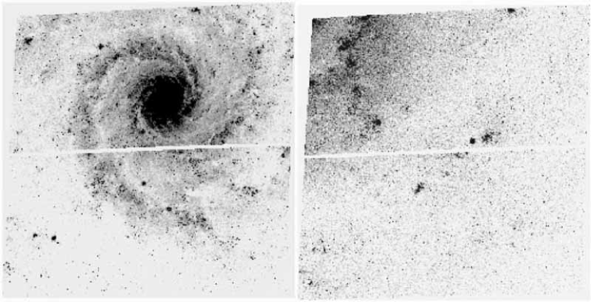
Figure 2: The ACS F435W images of NGC 628. The orientation is 67^∘ CCW from N in both images. The images are 210 arcsec in width.

The HST Advanced Camera for Surveys Wide Field Camera (ACS WFC) was used to image NGC 628 as part of a 37-orbit project on 7 nearby spiral galaxies to study star formation and structure (GO 10402; PI: Chandar). For the present study, we used images of NGC 628 centered on two different positions: a central one and an outer one (as shown in Figure 1). The central position was observed with four filters: B (F435W), V (F555W), I (F814W), and H$\alpha$ (F658N), while the outer position was imaged in B and V. Figure 2 shows the B-band images for the two positions, and Table 1 lists the positions and exposure times. The H$\alpha$ image was continuum-subtracted by combining the V and I images and scaling them so that the stars were eliminated in H$\alpha$. The images are 4211x4237 pixels, with a scale of 0.05 arcsec per px.

The distance to NGC 628 is assumed for simplicity to be 10 Mpc, using the value in Tully (1988), who derived 9.7 Mpc. Sohn & Davidge (1996) and Sharina et al. (1999) got $\sim 7$ Mpc from on red and blue supergiants. For 10 Mpc, the pixel size of 0.05 arcsec equals 2.42 pc.

3 Data Analysis

The images were Gaussian blurred in IRAF (Image Reduction and Analysis Facility) using the $\it{gauss}$ function with sigma (radii) of 1, 2, 4, 8, 16, 32, and 64 pixels in order to highlight features of different physical sizes.

The program $\it{SExtractor}$ was used to identify star-forming regions on each image. The resultant source maps were compared with the original images; the number of regions on the Gaussian-blurred source maps was counted by eye for comparison with what $\it{SExtractor}$ found, in order to check for proper settings. Thresholds equal to $3\sigma$, $5\sigma$, and $10\sigma$ above the background were a reasonable range. Limits were set so that the number of contiguous pixels above the threshold (the parameter $\it{detect\_minarea}$ in $\it{SExtractor}$) was required to be the square of the blur size. For example, for 2-pixel blurring, the objects had to have an area of at least 4 contiguous pixels; for 4-pixel blurring, the objects had to have an area of at least 16 pixels, and so on. Saturated stars were not included in the source counts.

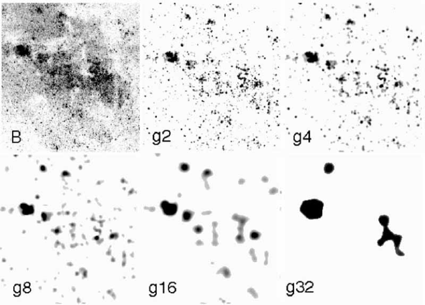
Figure 3: The F435W image (labeled B) of a star-forming complex in the central region is shown along with the $\it{SExtractor}$ object fields for Gauss-blurred images. The level of blurring is indicated by the number; g2 is a Gaussian blur of 2 pixels, etc.)

Figure 3 shows a B-band image of an enlarged portion of the Central Region. Also shown are the object fields generated by $\it{SExtractor}$ with a 5$\sigma$ threshold applied to images that are Gauss-blurred with 2, 4, 8, 16, and 32 pixels. $\it{SExtractor}$ finds all of the features that are larger than the blurring size.

4 Results

4.1 Size distribution function

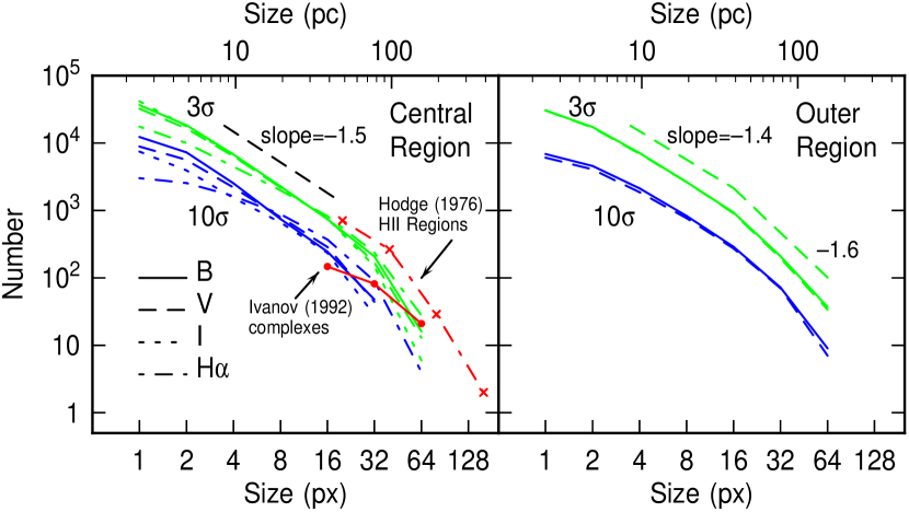
Figure 4: Cumulative size distributions for regions brighter than the 3$\sigma$ or 10$\sigma$ noise limits and larger than a given Gaussian-blur size. Different curves correspond to B,V,I, and H$\alpha$ images as indicated. The central region of NGC 628 was used for data on the left and the outer region was used for the right. Only B and V images are available for the outer region. The size is on the abscissa in units of pixels. The distributions are similar regardless of noise limit, filter, and position; all show a power law slope of $\sim-1.5$ with downward curvature at the upper end that is presumably from image edge effects. The cumulative distributions of size for HII regions and star complexes in this galaxy are also shown in the left-hand panel, with size converted to ACS pixels for comparison to the HST data.

Figure 4 shows the cumulative size distributions for star-forming regions. The Gaussian blur radius in pixels is plotted on the abscissa and the number of regions having radii greater than the Gaussian blur radius is plotted on the ordinate. The distributions are shown for the $3\sigma$ and $10\sigma$ limits in $\it{SExtractor}$ and for all of the available ACS passbands for the Outer and Central Regions, respectively. Star complexes and associations identified by eye on B-band ground-based images by Ivanov et al. (1992) are also included in this figure. The sizes given by Ivanov were divided by 2 to convert to radii and summed with radius bins equal to those of our ACS data. The smallest scale in the Ivanov compilation, $1.6^{\prime\prime}$, is close to the seeing limit, so the shallower slope of that distribution compared to ours may be the result of incompleteness. HII region sizes measured by Hodge (1976) on H$\alpha$ photographic plates of NGC 628 are included in Figure 4 too. The sizes were again divided by 2 and summed using the bins given in Hodge’s paper: $2^{\prime\prime}$, $4^{\prime\prime}$, $8^{\prime\prime}$, and $16^{\prime\prime}$, which correspond to 20, 40, 80, and 160 px in the ACS. The Hodge distribution of HII regions matches fairly well the distribution found here at the largest scales. Kennicutt & Hodge (1976) found from a power spectrum analysis of HII regions along the two main spiral arms that there is no preferred clump size.

Figure 4 indicates that the size distributions for emission features are slightly curved downward, as would be the case for a log-normal distribution, but resolution limits at small scales and spiral arms, disk thickness, or image edge effects at large scales could produce this curvature also (see Sect. 5).

There is little difference between the $3\sigma$ and $10\sigma$ features measured by $\it{SExtractor}$. This cutoff similarity, and the similarity in slope of the distribution functions for the different passbands, suggests that what we are measuring is the emission from hierarchically clustered stars, not the emission from a smooth disk viewed through hierarchically clustered dust holes. Dust holes should not give high brightness contrasts for all hole sizes like what we observe with the $10\sigma$ cutoff. The $3\sigma$ curves are higher than the $10\sigma$ curves because there are about 3 times as many features at $3\sigma$ above the noise than there are at $10\sigma$ above the noise. This means that the size distribution of the bright stellar cores (i.e., those $10\sigma$ above the noise) has about the same slope as the size distribution of the faint stellar envelopes (those $3\sigma$ above the noise). This similarity is consistent with the overall hierarchical nature of the star fields themselves, as shown by the near-power law size distributions. Generally, we expect the size distribution to get steeper as the cutoff brightness is increased because the objects selected at high cutoff levels are more and more limited to single emission points as a result of resolution limits and individual stars. This trend will be evident in the model below (see Fig. 7). The curves in Figure 4 are apparently not at such high cutoff levels.

The B, V, and I band size distributions are close to power laws all the way down to the smallest size, which corresponds to the angular resolution of the original image, about 1 pixel in radius. There is a slight drop at the smallest scale for the V-band image at $10\sigma$ in the Central Region, but no significant drop at the smallest scale for the other bands in this region. This is in contrast to the Outer Region, which has distinct deviations from power laws at the smallest scales in both B and V.

There are also deviations from power laws for the HII region size distributions at the smallest scale. The HII region distribution was measured only for the galaxy Central Region because the continuum subtraction for the H$\alpha$ image was made from a weighted average of the V and I bands, and there was no I band exposure for the outer region. The drop at small size for HII regions is much larger than the drop at small sizes for stellar structures in the V-band image at $10\sigma$. There is a factor of $\sim 10$ fewer HII regions with a size comparable to the image resolution than would be expected from an extrapolation of the power laws at larger scales. Recall that 1 and 2 pixels correspond to 2.7 and 5.4 pc at the assumed distance. Thus the drop suggests there are relatively few tiny HII regions. This result would be expected if most of the small HII regions represent only a short-lived phase in the expansion of a nebula around a massive star.

The slope of the power law for the size distribution is about $-1.5$, as suggested by the dashed lines in the figure. For a fractal of dimension $D$, the integrated number of objects having a size $\Sigma$ greater than some size $S$ scales as $N_{\Sigma}(\Sigma>S)\propto S^{-D}$. The number having a size between $S$ and $S+dS$ scales as $n_{S}(S)dS\propto S^{-1-D}dS$. The first function is the integral over the second, $N_{\Sigma}(\Sigma>S)=\int_{\Sigma}^{\infty}n_{S}(S)dS$. Taken at face value, the size distribution of stellar aggregates suggests a fractal distribution of stellar positions projected on the disk of the galaxy having a fractal dimension of $D=1.5$. This is less than 2, as expected, because the stellar aggregates do not completely fill the 2-dimensional plane of the galaxy disk. It is comparable to the fractal dimension of projected local interstellar clouds, which is $\sim 1.3$ (e.g., Falgarone et al. 1991), to the fractal dimension of HI ($D=1.2-1.5$) in the M81 group galaxies (Westpfahl et al. 1999), and to the fractal dimension of young stars in several dwarf galaxies (Crone 2005). Evidently, stars form in a fractal gas and preserve that pattern for some time.

4.2 Luminosity distribution functions

Figure 5 shows the luminosity functions of the stellar concentrations found in each Gaussian-blurred image. The ordinate is the count of regions having luminosities within a logarithmic interval of 0.5 on the abscissa. The abscissa is the flux of the various regions measured in total calibrated counts s^-1 on the ACS image. The calibration is such that a rate of 1 count s^-1 corresponds to an apparent magnitude of 25.15 mag using conversions in the on-line ACS data handbook. The blurring radius is indicated near each curve. The solid curves are for the B-band image with a $5\sigma$ lower limit in $\it{SExtractor}$. The curves nest inside each other at the high luminosity side because they all include the same regions at this end. The smaller regions become progressively more prominent as the resolution improves, filling out the lower luminosity end. The HII region luminosity function is shown as a dotted curve, using the 2-pixel Gaussian blurred image with a $5\sigma$ detection limit. It is significantly shallower than the stellar curves. The HII region luminosity function from Kennicutt, Edgar, & Hodge (1989) is also shown in Figure 5 as a dot-dash line. It was scaled to the flux count rate for the H$\alpha$ ACS image and is similar to the H$\alpha$ function found here but with lower count rate. The calibration conversion for H$\alpha$ is that one ACS count s^-1 corresponds to $1.6\times 10^{38}$ erg s^-1 at 10 Mpc.

The fraction of the total B-band emission in the regions counted in Figure 5 decreases with increasing blur radius. For blurs of 1, 2, 4, 8, 16, 32 and 64 pixels, this fraction is 0.16, 0.13, 0.10, 0.07, 0.04, 0.01, and 0.0003. This is consistent with the decreasing integrals under the curves in Figure 5. The decrease confirms our impression from Figure 3 that the regions are not strictly hierarchically nested with all the small regions inside the large regions. If this were the case, then every region would be present in all blur images, with the small region fluxes contributing to the large regions at large blur radius; as a result, the fractional flux would be constant with blur radius. Instead, there are numerous small regions independent of the large regions. These small regions get lost at large blur radius and drop below our detection cutoff, causing the integrated flux to decrease with blur radius. We note that our models in Section 5 look the same as the observations in the sense that there are numerous small regions independent of the large regions, in addition to small regions embedded inside the large regions.

The slope of the luminosity distribution function for stellar aggregates is $\sim-1$ on this log-log histogram. This means the luminosity distribution is approximately $N_{log}(L)d\log L\propto L^{-1}d\log L$, or in linear intervals, $n_{L}(L)dL\propto L^{-2}dL$.

This slope is typical for the luminosity distributions of standard (“open”) clusters, as found in many studies. Kennicutt & Hodge (1980) found a similar distribution for HII region luminosities in NGC 628 from ground-based images, which did not include the central 1^′ of the galaxy and included only nebulae larger than about 4^′′. Lelievre & Roy (2000) found a slope of $\sim{-1.6}$ on a cumulative luminosity function, which implies the same slope of $-1.6$ on a histogram with logarithmic binning, as in our Fig. 5.

The slope of the luminosity function for extended star-forming regions should not be viewed as a continuation of the slope of the luminosity functions for young clusters and HII regions, even though the numerical values of these slopes are about the same. The extended distribution found here has a much larger scale than any individual cluster or exciting source of an HII region, and the larger region is likely to be significantly evolved, as for a typical star complex (Efremov 1995). Thus, the luminosity of an extended region is not directly proportional to its mass, as it is for a young cluster. The large regions are also likely to be a composite of several smaller regions observed in projection through the galaxy, unlike individual clusters and HII regions. We return to these points in section 5 where fractal models reproduce the observed distributions.

The slope of the luminosity function, combined with the slope of the size distribution, gives the relation between luminosity and size. Taking $n_{S}(S)dS\propto S^{-2.5}dS$ and $n_{L}(L)dL\propto L^{-2}dL$, and assuming a one-to-one correspondence where $n_{S}(S)dS=n_{L}(L)dL$, gives $S^{-2.5}dS\propto L^{-2}dL$, from which we derive $L\propto S^{1.5}$. This power is another definition of the fractal dimension because a fractal has its content (mass, luminosity, number of objects, etc.) increase with size to a power that is the fractal dimension, $D=1.5$ in this case. The luminosity-size relation implies that the projected stellar luminosity density decreases for larger regions as $LS^{-2}\propto S^{-0.5}$. This is a sensible result because larger stellar aggregates have more open space.

5 Models

Three-dimensional fractal models of density distributions having an approximately power-law power spectrum like the ISM (e.g., Dickey et al. 2001) and a log-normal density probability distribution function, as in turbulence simulations (Vázquez-Semadeni 1994; Elmegreen & Scalo 2004), can reproduce the observed $M^{-1}d\log M$ distribution of stellar clusters and the more shallow distribution of molecular clouds (Elmegreen 2002; 2004). The shallow distribution comes from the same fractal as the steep distribution, but with a lower density cutoff (see also Sanchez, Alfaro & Pérez 2005). Figure 6 (reproduced from Elmegreen 2004) shows this result by plotting the slope of the clump mass function versus the power $\beta$ of the power spectrum, generated from the average of many random fractal models, for various lower limits to the density measured in terms of the peak density in the fractal. For a 3D Kolmogorov-type spectrum, with $\beta=-11/3$ (vertical dashed line), the dense cores have an $M^{-1}\log M$ distribution like star clusters and the low density regions have shallower distributions, $\sim M^{-0.5}d\log M$, like molecular clouds (e.g., Solomon et al. 1987). Thus a fractal, log-normal ISM, such as that generated in turbulence simulations, can reproduce both the GMC and the cluster mass functions.

Our observations here show similar power-law distributions, but the measured quantities are different. First, the observations consider fairly large regions (the 64 px blur corresponds to objects larger than 155 pc) and not individual clusters. Second, these regions are observed in projection through a galaxy disk and are probably not spherical anyway. To simulate this case, we make a fractal Brownian motion model for the density distribution in a face-on slab with a thin Gaussian profile on the line of sight. This is made by first filling one-half of a $210^{3}$ cube in wavenumber space ($k_{x},k_{y},k_{z}$) with random complex numbers uniformly distributed from 0 to 1, and then multiplying each number by $k^{-\beta/2}$ for $k^{2}=k_{x}^{2}+k_{y}^{2}+k_{z}^{2}$. The inverse Fourier transform of this distribution is a multifractal density cube in real space with a power spectrum slope $-\beta$. It has a Gaussian density probability distribution function (pdf), so we exponentiate it to give another density distribution which has a log-normal density pdf. The power spectrum changes a little at low $k$ after this exponentiation, but not noticeably at intermediate to high $k$ (see Weinberg & Cole 1992 for corrections to recover the original power law). Our galaxy model uses the inner $180^{3}$ cube of this density distribution to avoid periodic edge effects, and multiplies it by a Gaussian along the line-of-sight $z$ axis, centered at the $z$ midplane and having a dispersion of 18 pixels. Thus the model is a face-on multifractal slab (x,y plane) with a Gaussian line-of-sight distribution for the mean density. It has a ratio of width to effective depth equal to 5. In a final step, the galaxy model was summed over the line-of-sight $z$ to make the projected multifractal galaxy.

We are interested in the size and mass distributions of the densest clouds in this multifractal galaxy model. We define a cloud as an isolated but internally connected region with all pixel values above a certain cutoff. If the cutoff is too low, then the regions are so large that they overlap and form only one big cloud. If the cutoff is too high, then the regions are small and there are only a few of them. We found that cutoff values in the range between 0.3 and 0.6 times the peak density gave good samples of clouds for the size and mass distribution functions. The cloud boundaries are identified automatically by a random walk. More details are in Elmegreen (2002). To determine statistically significant distribution functions, we made 90 random models for each pair of parameters, $\beta$ and the cutoff value, and then plotted the total count of clouds from all of these models. Each model has a different peak density so the cutoff varies a little from model to model in absolute terms for each parameter pair.

The cumulative size and mass distribution functions are shown in Figures 7 and 8. Each figure has four panels, one for each $\beta$, the slope of the power spectrum of the multifractal. In each panel there are 2, 3, or 4 curves corresponding to the four cutoff values. The low cutoff values for low $\beta$ are not plotted because these clouds overlapped severely. The value of $\beta=3.66$ is appropriate for the velocity power spectrum of three-dimensional Kolmogorov turbulence; $\beta=2.66$ for two-dimensional Kolmogorov turbulence as might be expected in a thin galaxy disk. We show these values for this reason plus the two other values on either side. The panel for $\beta=3.66$ has crosses representing the counts observed in B-band for the $3\sigma$ limit (from the left hand panel of Fig. 4).

The cumulative size distribution in Figure 7 plots the number of clouds larger than the size given on the abscissa, in units of model pixels. The size of a cloud is defined to be the density-weighted two-dimensional rms dispersion of all the projected pixels in the cloud. The rms size of a single pixel cloud is taken to be 0.707 pixel units. The mass is defined to be the sum of the densities in the cloud.

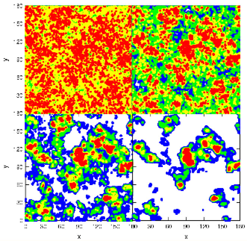
Figure 9: Images of projected fractal galaxies for four different $\beta$ showing projected density as color. The top left has $\beta=1.66$, top right $\beta=2.66$, lower left $\beta=3.66$ and lower right $\beta=4.66$. Blue regions have projected densities between 0.3 and 0.4 of the peak, green between 0.4 and 0.5, yellow between 0.5 and 0.6, and red greater than 0.6. (degraded resolution for astroph)

Figure 9 shows an example of each map for the four different power spectrum slopes, $\beta$. The four cutoff levels are indicated by color: blue pixels are between 0.3 and 0.4 of the peak, green between 0.4 and 0.5, yellow between 0.5 and 0.6, and red greater than 0.6. The order in $\beta$ of the panels is the same as in the previous two figures. The random numbers are the same for each panel, so the designs are similar; the only difference is the value of $\beta$.

The cumulative size distributions in Figure 7 curve downward a little, with an average slope at mid-range of approximately $-1.5$, as indicated by the solid line. The slopes are systematically steeper for higher cutoff values, and the counts are lower too. The counts also decrease slightly with increasing $\beta$. The curvature at large size is from edge effects: the rms size of the whole projected square is 73 px. The mass functions in Figure 8 are also somewhat curved from edge or spiral arm effects but they have a power law middle range with a slope between $-0.5$ and $-1$ for these value of $\beta$.

The models agree fairly well with the observations (crosses in Fig. 7), suggesting that the size distribution for stellar aggregates in NGC 628 (Fig. 4) results from a multifractal ISM where star formation occurs in the gas peaks. The model size distributions are relatively insensitive to the power spectrum, but the observed ISM slope $\beta\sim 3$ (e.g., Stanimirovic et al. 1999; Dickey et al. 2001; Elmegreen, Kim, & Staveley-Smith 2001) gives about the right size distribution for stellar aggregates.

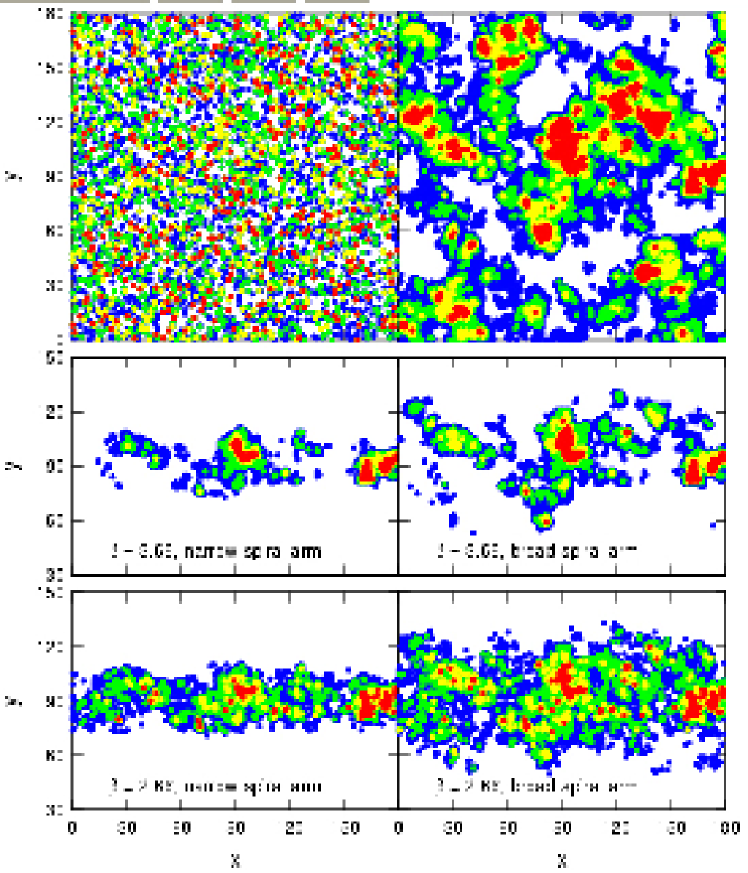
Figure 10: Images of alternative models for projected fractal galaxies, all of which have a Gaussian profile of average density on the line of sight with a dispersion of 18 pixels. Top left: purely random values are used for the density prior to multiplication by the line of sight Gaussian. Top right: $\beta=3.66$ model reproduced from Fig. 9. Middle left: $\beta=3.66$ model with a Gaussian profile in the $y$ direction having a dispersion equal to the dispersion of the line of sight depth. Middle right: $\beta=3.66$ with a $y$ dispersion twice as large. Bottom left and right: $\beta=2.66$ with the same two $y$ dispersions. In the top two panels, the blue regions have projected densities between 0.3 and 0.4 of the peak, green between 0.4 and 0.5, yellow between 0.5 and 0.6, and red greater than 0.6. In the bottom four panels, the density limits are shifted because the peak density is smaller on average when the models are smaller: blue is 0.4-0.5 times the peak, green is 0.5-0.6, yellow is 0.6-0.7, and red is greater than 0.7 times the peak. (degraded resolution for astroph)

Other types of models were run for comparison. A model galaxy where every pixel in real space was noise, rather than the Fourier transform of noise with a power-law taper, produced a size spectrum that was approximately a delta function centered at the lowest size. This model had the same size and Gaussian profile on the line of sight as the fractal models, and was also viewed in projection, but there were no large-scale correlations that could produce the appearance of OB associations and star complexes and, hence, no statistically significant regions larger than a pixel. A map of this model is shown at the top left of Figure 10. The $\beta=3.66$ model from the lower left of Figure 9 is shown at the top right for comparison.

A third model used the same fractal algorithm as above, with the Gaussian multiplier on the line of sight as before, but now there was also a Gaussian multiplier along one of the projected directions, vertical on the page. Four versions of this model are shown in the center ($\beta=3.66$) and bottom ($\beta=2.66$) of Figure 10. On the left of each, the vertical dispersion is equal to the dispersion in depth, and on the right, the vertical dispersion is twice the dispersion in depth. These models are meant to represent spiral arms in the sense that the star complexes are confined in one of the in-plane directions. The size and mass distributions for this spiral arm model are shown in Figure 11. The distributions are similar to those in Figures 7 and 8 but because the areas are smaller for the spiral models, the counts and masses of objects are all smaller, as are the upper size and mass limits. The implication is that the spiral arms in NGC 628 should not affect our conclusions regarding the slope of the size, mass, and luminosity distribution functions. However, the minimum physical size where the distribution function in Figure 7 begins to fall off is only 77 pc (32 px), which is more like a spiral arm width than the galaxy image size ($\sim 10$ kpc). Thus the large-scale fall off in the spiral arm models is probably a more reasonable explanation for the observed fall-off than the large-scale fall off from image size limitations in Figure 9.

Many other models can be imagined but they should not change the overall size and mass distributions much as long as the density is spatially correlated as in the fractal models with the Kolmogorov-like values of slope for the power spectrum. For example, the difference between star complexes with large central clusters and star complexes without large central clusters (e.g., Maíz-Apellániz 2001), or the difference between centrally concentrated complexes versus ring-like complexes, should not be as nearly as great as the difference between correlated and un-correlated models. Models in Elmegreen & Elmegreen (2001) using randomly placed clusters with a power law intrinsic size distribution also failed to match the observations.

The preferred model mass distributions shown in Figure 8 are not the same as the observed luminosity distribution except for very low $\beta$. Low $\beta$ puts relatively more power at high spatial frequency, making relatively more small clouds and steepening the mass function (Stützki et al. 1998). This trend with $\beta$ is also apparent in Figure 6 for three-dimensional clouds. For realistic $\beta$ in the range from 2.6 to 3.6, the slope of the projected mass distribution for logarithmic intervals is between $-0.55$ and $-0.75$ in Figure 8, clearly shallower than the observed luminosity distribution in Figure 5, where the slope is $\sim-1$. We believe that the difference lies in the luminosity evolution of associations and star complexes over time, as shown by the following considerations.

Suppose the mass distribution in the model has a slope $-\mu$ for linear intervals of mass, and the size distribution has a slope $-1-D$ for linear intervals of size (as in Sect. 4.1). Then the relation between mass $M$ and size $S$ is $M\propto S^{\Delta}$ where $\Delta=D/(\mu-1)$. The models suggest $D\sim 1.5$ and $\mu$ is between 1.55 and 1.75, so $\Delta$ is between 2.7 and 2. Suppose also that the average age scales with the size of the region as $T\propto S^{\tau}$, as found in the LMC (Efremov & Elmegreen 1998), where $\tau\sim 0.5$. This age scaling could result from turbulence as could the whole hierarchical pattern, provided $T\propto S/V$ (Elmegreen 2000) and the velocity dispersion $V$ scales with $S^{0.5}$ (e.g., Larson 1981). Finally, suppose that the luminosity of a region begins in proportion to its mass and then decays like a power law with time: $L\propto MT^{-\epsilon}$. From Figure 13 in Girardi et al. (1995), we obtain $\epsilon\sim 0.6$. Boutloukus & Lamers (2003) got $\epsilon=0.648$ for the Starburst99 models. A slightly different value, $\epsilon=0.75$, was determined from BC01 models (Bruzual & Charlot 2003) by Larsen (2002). It follows that luminosity and mass are related by $L\propto M^{1-\tau\epsilon/\Delta}$. Equating the distribution functions, $n(L)dL=n(M)dM$, gives the desired result:

$$n(L)=n(M){{dM}\over{dL}}\propto M^{-\mu+\tau\epsilon/\Delta}\propto L^{-\lambda}$$ (1)

where

$$\lambda={{\mu-\tau\epsilon/\Delta}\over{1-\tau\epsilon/\Delta}}$$ (2)

With the above parameters, the slope of the luminosity function, $-\lambda$, should range between $-1.6$ and $-1.9$ for $\mu=1.55$ and $1.75$, respectively (the three values of $\epsilon$ give about the same results). The latter $\lambda$ is reasonably close to the observed slope in Figure 5.

6 Conclusions

HST observations of the nearby spiral galaxy NGC 628 reveal a regular hierarchy of structures for the brightest stars. These structures are of a type previously studied individually as star complexes, OB associations, OB subgroups, and so on, but in the present study they all blend together without distinction as parts of a nearly scale-free distribution of young stellar objects. Such scale-free distributions have now been found using many different techniques. The structure implies that stars form in the densest regions of a pervasive multi-fractal gas. The most likely origin for this gas structure is a scale-free forcing of gas motions and compressions by turbulence and self-gravity. The largest scale appears, in other studies, to be approximately the ambient Jeans length in a galaxy, suggesting that self-gravity is a primary driver for star formation, with the substructure provided by self-gravity, turbulence, and other forced motions.

The luminosity distribution of the stellar aggregates is approximately a power law, like the size distribution. The observations show some downward curvature in both of these distributions, suggesting functions more like log-normals than strict power laws, but observational limitations at the small and large ends could produce this curvature artificially. Thus we cannot determine yet the full functional form of the distributions. Hierarchical structure is revealed because the high resolution and wide field of the HST observations display a large dynamic range for spatial scales.

Multifractal models with some resemblance to the density structures produced by turbulence can reproduce the observed size distribution function in NGC 628. The model mass functions are more shallow than the observed luminosity function, but this could be the result of luminosity fading with age if the larger regions are older on average, in proportional to the square root of their size. The fractal dimension of the stellar aggregates is about $-1.5$, similar to the fractal dimension found elsewhere for gas distributions and other star fields.

This research was supported by NASA grant HST-GO-10402-A. D.M.E. gratefully acknowledges the hospitality of the Space Telescope Science Institute staff during her visit as a Caroline Herschel Visitor in October 2005, and thanks Benne Holwerda for advice on using $\it{SExtractor}$.

Table 1: Observations

	Outer Region	Central Region
RA,Dec	01 36 30.98, +15 48 50.23	01 36 40.60, +15 46 39.00
Filter	Exposure (sec)	Exposure (sec)
F435W	1200	1358
F555W	1000	858
F658N	-	1422
F814W	-	922

Figure 1: The Digital Sky Survey B-band image of NGC 628 with ACS grids for positions 1 (Outer Region) and 3 (Central Region). North is up. The ACS boxes are 210 arcsec across.

Figure 5: Number distributions of flux count rates in logarithmic intervals for stellar aggregates observed in B-band and H$\alpha$ (dotted line) ACS images of the central region (left), and for the B-band image of the outer region (right). Each solid curve is for a different Gaussian blur size limit in B-band, as indicated by the associated numbers of pixels for the blur. For the H$\alpha$ curve, only the 2-pixel Gaussian blur distribution is shown (the others have a nested structure similar to that of the B band). The slopes at high flux are all similar and about equal to $-1$ as indicated by the solid line. The curves turn over at the faint end because of the Gaussian blur. Flux is defined to be the sum of the count rates for the pixels in each region, in units of electrons per second. A count rate of 1 for the B band corresponds to an apparent magnitude of 25.15; a count rate of 1 in H$\alpha$ corresponds to $1.6\times 10^{38}$ erg s^-1.

Figure 6: Slopes of the mass distribution functions for clouds in three dimensional fractal Brownian motion models. The abscissa is the slope of the noise power spectrum used to generate the models. The ordinate is the slope of the cloud number distribution calculated for equal bins in the log of the mass. The power spectrum slope for 3D Kolmogorov turbulence is indicated by the vertical dashed line. The typical slope of the initial cluster mass function (ICMF) is indicated by a horizontal dotted line. Different curves are for different density cutoffs in the definition of a cloud. Low density cutoffs give a shallower slope, $\sim-0.5$, which is similar to the observed slope of the molecular cloud mass distribution. High density cutoffs give steeper slopes, like the ICMF.

Figure 7: Cumulative projected size distribution functions for clouds in fractal Brownian motion models of face-on thin disks. The abscissa is the size of the cloud in pixels and the ordinate is the number of clouds larger than this size in the model. The model disks are projections of multifractal density cubes with a Gaussian multiplier for the average density on the line of sight. The aspect ratio of the disk is 5:1. Each panel is for a different slope $\beta$ of the power spectrum for the noise in the fractal Brownian motion model. Different curves in each panel are for different density cutoffs in the definition of a cloud. A fiducial slope of $-1.5$ is indicated by a line. The crosses represent the observed size distribution from Fig. 4 for B-band at the 3$\sigma$ limit.

Figure 8: Mass distributions of projected clouds in the fractal galaxy model. Each panel is a different $\beta$, which is the slope of the power spectrum, and each line in a panel is a different cutoff density for the definition of a cloud. The low $\beta$ panels do not show the results for low cutoff densities because in these cases most of the gas blends into only a few big clouds. A fiducial slope of $-1$ is shown.

Figure 11: Size and mass distribution for $\beta=3.66$ and $\beta=2.66$ models with Gaussian profiles in one dimension of the projected plane, to simulate spiral arms. In each panel, the solid, dashed, and dotted line types correspond to density limits greater than 0.5 times the peak, 0.6 times the peak, and 0.7 times the peak. The top curves for each type correspond to broad arms with Gaussian dispersions of 36 pixels and the bottom curves correspond to narrow arms with dispersions of 18 pixels. The curves here are nearly the same as in Figs. 7 and 8, except for a downward shift in each case.

References

- (1) Bally, J., Cunningham, N., Moeckel, N., & Smith, N. 2005, IAU Symposium 227, 12
- (2) Bastian, N., Gieles, M., Efremov, Yu. N., & Lamers, H. J. G. L. M. 2005, A&A, 443, 79
- (3) Battinelli, P., Efremov, Y., & Magnier, E.A. 1996, A&A, 314, 51
- (4) Bonnell, I. A., Bate, M. R., & Vine, S. G. 2003, MNRAS, 343, 413
- (5) Boutloukos, S.G. & Lamers, H.J.G.L.M. 2003, MNRAS, 338, 717
- (6) Brandeker, A., Jayawardhana, R., & Najita, J. 2003, AJ, 126, 2009
- (7) Bresolin, F., Kennicutt, R.C., Jr., Ferrarese, L., Gibson, B. K., Graham, J. A., Macri, L. M., Phelps, R. L., Rawson, D. M., Sakai, S., Silbermann, N. A., and 2 coauthors 1998, AJ, 116, 119
- (8) Bruzual, G., & Charlot, S. 2003, MNRAS, 344, 1000
- (9) Chen, Y., & Crone, M.M. 2005, AAS, 20711305
- (10) Crone, M.M. 2005, AAS, 20711315
- (11) Dahm, S. E., & Simon, T. 2005, AJ, 129, 829
- (12) Dickey, J.M., McClure-Griffiths, N.M., Stanimirovic, S., Gaensler, B.M, & Green, A.J, 2001, ApJ, 561, 264
- (13) Efremov, Y.N. 1995, AJ, 110, 2757
- (14) Efremov, Y.N., & Elmegreen, B.G. 1998, MNRAS, 299, 588
- (15) Elmegreen, B.G. 2000, ApJ, 530, 277
- (16) Elmegreen, B.G., Efremov, Y.N., Pudritz, R., & Zinnecker, H. 2000, in Protostars and Planets IV, ed. V. G. Mannings, A. P. Boss, & S. S. Russell, Tucson: Univ. Arizona Press, 179
- (17) Elmegreen, B.G. & Elmegreen, D. M. 2001, AJ, 121, 1507
- (18) Elmegreen, B.G., Kim, S., & Staveley-Smith, L. 2001, ApJ, 548, 749
- (19) Elmegreen, B.G. 2002, ApJ, 564, 773
- (20) Elmegreen, B.G., Elmegreen, D.M., & Leitner, S.N. 2003, ApJ, 590, 271
- (21) Elmegreen, B.G., Leitner, S.N., Elmegreen, D.M., & Cuillandre, J.-C. 2003, ApJ, 593, 333
- (22) Elmegreen, B. C. 2004, in The Formation and Evolution of Massive Young Star Clusters, ASP Conference Series, Vol. 322, eds. H.J.G.L.M. Lamers, L.J. Smith, & A. Nota, San Francisco: Astronomical Society of the Pacific, 277
- (23) Elmegreen, B.G. 2005, in The many scales in the Universe - JENAM 2004 Astrophysics Reviews, from the Joint European and National Astronomical Meeting, Kluwer Academic Publishers, ed. Jose Carlos del Toro Iniesta, et al., in press
- (24) Elmegreen, B.G., & Scalo, J. 2004, ARAA, 42, 211
- (25) Falgarone, E., Phillips, T., & Walker, C.K. 1991, ApJ, 378, 186
- (26) Feitzinger, J. V., & Galinski, T. 1987, A&A, 179, 249
- (27) Feitzinger, J. V., & Braunsfurth, E. 1984, A&A, 139, 104
- (28) Girardi, L., Chiosi, C., Bertelli, G., Bressan, A. 1995, A&A, 298, 87
- (29) Gomez, M., Hartmann, L., Kenyon, S. J., & Hewett, R. 1993, AJ, 105, 1927
- (30) Gusev, A. S. 2002, A&AT, 21, 75
- (31) Harris, J., & Zaritsky, D. 1999, AJ, 117, 2831
- (32) Heydari-Malayeri, M., Charmandaris, V., Deharveng, L., Rosa, M.R., Schaerer, D., & Zinnecker, H. 2001, A&A, 372, 495
- (33) Hodge, P.W. 1976, ApJ, 205, 728
- (34) Ivanov, G.R. 2005, PASRB, 4, 75
- (35) Ivanov, G.R., Popravko, G., Efremov, Yu.N., Tichonov, N.A., & Karachentsev, I.D. 1992, A&A Supp. Ser., 96, 645
- (36) Kennicutt, R.C. & Hodge, P.W. 1976, ApJ, 207, 36
- (37) Kennicutt, R.C. & Hodge, P.W. 1980, ApJ, 241, 573
- (38) Kennicutt, R.C., Edgar, B.K., & Hodge, P.W. 1989, ApJ, 337, 761
- (39) Krumholz, M.R. & McKee, C.F. 2005, ApJ, 630, 250
- (40) Larson, R.B. 1981, MNRAS, 194, 809
- (41) Larsen, S. S. 2002, AJ, 124, 1393
- (42) Lelievre, M., & Roy, J.-R. 2000, AJ, 120, 1306
- (43) Maíz-Apellániz, J. 2001, ApJ, 563, 151
- (44) Maragoudaki, F., Kontizas, M., Kontizas, E., Dapergolas, A., & Morgan, D.H. 1998, A&A, 338, L29
- (45) Nanda Kumar, M.S., Kamath, U.S., & Davis, C.J. 2004, MNRAS, 353, 1025
- (46) Oey, M.S., King, N.L., & Parker, J.W. 2004, AJ, 127, 1632
- (47) Oey, M.S., Watson, A.M., Kern, K., & Walth, G.L. 2005, AJ, 129, 393
- (48) Pietrzyn’ski, G., Gieren, W., Fouqu , P., & Pont, F.A. 2001, A&A, 371, 497
- (49) Sanchez, N., Alfaro, E.J., & Pérez, E. 2005, astroph/0512243
- (50) Sharina, M.E., Karachentsev, I.D., & Tikhonov, N.A. 1999, Astron. Letters, 25, 322
- (51) Smith, N., Bally, J., Shuping, R. Y., Morris, M., & Kassis, M. 2005, AJ, 130, 1763
- (52) Smith, M. D., Gredel, R., Khanzadyan, T., & Stankeinst, T. 2005, MmSAI, 76, 247
- (53) Sohn, Y.-J., Davidge, T.J. 1996, AJ, 111, 2280
- (54) Solomon, P.M., Rivolo, A.R., Barrett, J., & Yahil A. 1987, ApJ, 319, 730
- (55) Stanimirovic, S., Staveley-Smith, L., Dickey, J.M., Sault, R.J., & Snowden, S.L. 1999. MNRAS, 302, 417
- (56) Stützki, J., Bensch, F., Heithausen, A., Ossenkopf, V., & Zielinsky, M. 1998, A&A, 336, 697
- (57) Testi, L., Sargent, A.I., Olmi, L., & Onello, J.S., 2000, ApJ, 540, L53
- (58) Tully, R.B. 1988, Nearby Galaxies Catalog, Cambridge Univ. Press
- (59) Vázquez-Semadeni, E. 1994, ApJ, 423, 681
- (60) Weinberg, D. H., & Cole, S. 1992, MNRAS, 259, 652
- (61) Westpfahl, D.J., Coleman, P.H., Alexander, J., Tongue, T. 1999, AJ, 117, 868
- (62) Zhang, Q., Fall, S. M., & Whitmore, B. C. 2001, ApJ, 561, 727