The coherence of kHz quasi-periodic oscillations in the X-rays from accreting neutron stars

Abstract

We study in a systematic way the quality factor of the lower and upper kHz QPOs in a sample of low luminosity neutron star X-ray binaries, showing both QPOs varying over a wide frequency range. The sample includes 4U 1636–536, 4U 1608–522, 4U 1735–44, 4U 1728–34, 4U 1820–303 and 4U 0614+09. We find that all sources except 4U 0614+091 show evidence of a drop in the quality factor of their lower kHz QPOs at high frequency. For 4U 0614+091 only the rising part of the quality factor versus frequency curve has been sampled so far. At the same time, in all sources but 4U 1728–34, the quality factor of the upper kilo-Hz QPO increases all the way to the highest detectable frequencies. We show that the high-frequency behaviours of both the lower and upper kHz QPO quality factors are consistent with what is expected if the drop is produced by the approach of an active oscillating region to the innermost stable circular orbit: the existence of which is a key feature of General Relativity in the strong field regime. Within this interpretation, our results imply gravitational masses around $2M_{\odot}$ for the neutron stars in those systems.

1 Introduction

Kilohertz Quasi-Periodic Oscillations (kHz QPOs) have now been detected by the Rossi X-ray Timing Explorer (RXTE, Bradt et al. 1993) from about 25 neutron star low-mass X-ray binaries (van der Klis 2006 and references therein). These signals, whose timescales correspond to the dynamical times of the innermost regions of the accretion flow, have triggered much interest because they may carry imprints of strong field general relativity, such as the existence of an innermost stable circular orbit (ISCO) around a sufficiently compact neutron star. For instance, a drop in the amplitude and quality factor of the QPOs at some limiting frequency was proposed as a possible signature of the ISCO (e.g., Miller, Lamb, & Psaltis 1998).

Following this idea, we studied in a systematic way the QPO properties of 4U 1636–536, with emphasis on the dependency of the quality factor ($Q\equiv\nu/{\rm FWHM}$) and amplitude with frequency (Barret, Olive, & Miller 2005a,b). We have thus shown that the lower and upper kHz QPOs of 4U 1636–536 follow two distinct tracks in a Q versus frequency plot. The quality factor of the lower kHz QPO increases with frequency up to a maximum of $Q\sim 200$ at $\sim 850$ Hz, then drops precipitously to $Q\sim 50$ at the highest detected frequencies $\nu_{\rm lower}\sim 920$ Hz (a similar behaviour was seen earlier from 4U1608-52, Barret et al. 2005c) On the other hand, the quality factor of the upper kHz QPO increases steadily all the way to the highest detectable QPO frequency, although the quality factor is lower than for the lower QPO. The rms amplitudes of both the upper and lower kHz QPOs decrease steadily towards higher frequencies.

In this paper, we extend the analysis carried out for 4U 1636–536 to all low-luminosity neutron star binaries for which kHz QPOs have been detected over a large range of frequencies. The sample includes: 4U 1636–536, 4U 1608–522, 4U 1820–303, 4U 1735–44, 4U 1728–34, 4U 0614+09. An exhaustive list of references on QPOs from these sources is available in van der Klis (2006). In § 2 we describe our analysis procedure, and in § 3 we discuss the implications of our results and show how the high-frequency dropoff in $Q$ can be accommodated quantitatively in a toy model based on the approach to the ISCO.

2 Data analysis

For the purpose of this paper, we have retrieved all science event files from the RXTE archives up to the end of 2004 for all six sources. The files are identified with their observation identifier (obs ID) following the RXTE convention. An Obs ID identifies a temporally contiguous collection of data from a single pointing. Only files with time resolution better than or equal to 250 micro-seconds and exposure times larger than 600 seconds are considered. No filtering on the raw data is performed, which means that all photons are used in the analysis. Type I X-ray bursts and data gaps are removed from the files.

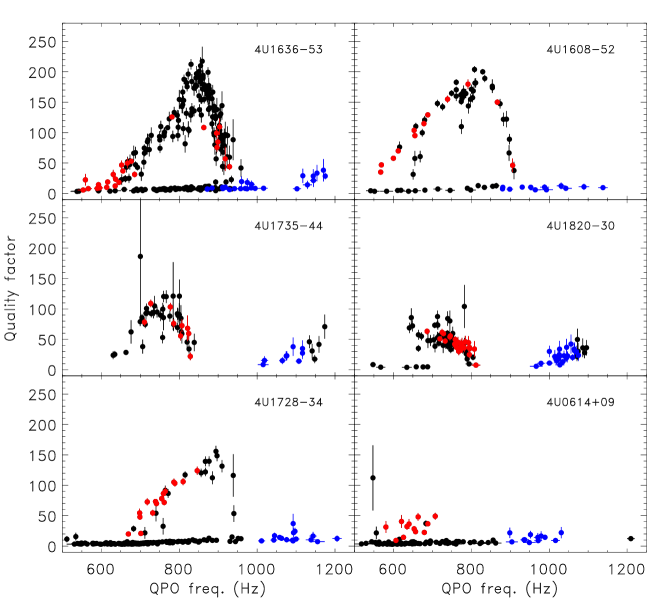
Figure 1: Quality factor versus frequency of all fitted QPOs: red circles identify fitted lower QPOs, blue circles identify fitted upper QPOs, black circles correspond to single QPOs. Each data point represents the average over a continuous data segment.

For each file identified with its Obs ID, we have computed Leahy normalized Fourier power density spectra (PDS) between 1 and 2048 Hz over 8 s intervals (with a 1 Hz resolution). $N$ 8-second PDS are thus computed. $N$ is typically around 400 in most files, whose duration $\sim 3200$ is consistent with the orbital period of the RXTE spacecraft. A Fourier power spectrum averaging the $N$ PDS is first computed. This averaged PDS is then searched for a QPO using a scanning technique which looks for peak excesses above the Poisson counting noise level (Boirin et al. 2000). No fit is performed at this stage as the scanning procedure returns the centroid frequency of each excess and an approximation of its spread in frequency (a rough measure of its total width). In case of the presence of two excesses, the one with the higher significance is considered: its centroid frequency is $\nu_{0}$ and its spread is $w_{0}$.

We now wish to attribute to all $N$ PDS the best estimate of the instantaneous QPO frequency $\nu_{qpo_{\rm 1\dots N}}$ to apply later on the shift-and-add technique. To start, $\nu_{qpo_{\rm 1\dots N}}$ is set to $\nu_{0}$. We define a window of 25 Hz on both sides of the excess centered at $\nu_{0}$ and recursively search for excesses over time intervals of shorter and shorter durations, i.e. in a smaller and smaller number of 8 second PDS averages. More specifically, in the first iteration, we thus consider two consecutive time intervals averaging the 8-sec PDS from number 1 to $N/2$ to produce PDS_1,1 and the 8-sec PDS from number $N/2+1$ to $N$ to produce PDS_1,2. In PDS_1,1 and PDS_1,2, we search for peak excesses between $\nu_{0}-w_{0}/2-25$ Hz and $\nu_{0}+w_{0}/2+25$ Hz, still above the Poisson counting noise level at the 4$\sigma$ level. For instance, if an excess is detected PDS_1,1 at a frequency $\nu_{1,1}$ (spread $w_{1,1}$), then we set $\nu_{qpo_{\rm 1\dots N/2}}$ to $\nu_{1,1}$ before the next iteration. If on the other hand, no excess is detected in PDS_1,2, then $\nu_{qpo_{\rm N/2+1\dots N}}$ remains unchanged at $\nu_{0}$. In the next iteration, we repeat the procedure considering two further intervals averaging the 8-sec PDS from number 1 to $N/4$ to produce PDS_2,1 and the 8-sec PDS from number $N/4+1$ to $N/2$ to produce PDS_2,2, and search in both PDS an excess between $\nu_{1,1}-w_{1,1}/2-25$ Hz and $\nu_{1,1}+w_{1,1}/2+25$ Hz. The tracking procedure stops when no more excess is detected in any of the intervals analyzed. At the end, the procedure thus returns the best possible estimate of the instantaneous QPO frequency in each 8 second PDS. We have checked through simulations of a QPO signal of varying frequency and of amplitude similar to the real data that this procedure follows with great accuracy the changes in frequency.

In order to reduce the contribution of the long term frequency drift to the broadening of the QPO profile, within a data file, we then shift-and-add (Méndez et al. 1998) the individual 8 second PDS to the mean QPO frequency over the file. The shifted and added PDS is then searched for QPOs with the scanning routine. A quality check is performed at this stage with the scanning routine to verify that the tracked QPO in the resulting PDS has a centroid frequency consistent with $\nu_{0}$ and a spread smaller than $w_{0}$. Either one or two QPOs are then fitted with a Lorentzian of three parameters (frequency, full width at half maximum, and normalization) to which a constant is added to account for the counting noise level (close to 2.0 in a Leahy normalized PDS). The fitting is carried with the XSPEC 11.3.2 spectral package (Arnaud 1996), taking advantage of the robustness of its fitting procedures (including the error computations). Next, we keep QPOs which are detected above $2.5\sigma$ (the significance being defined as the integral of the Lorentzian divided by its error), above 500 Hz, with a quality factor larger than 3.

In Figure 1, we show the quality factor of the QPOs detected for all six sources. Although with fewer details than for 4U 1636–536, the same trends are present for all the other sources as well. In particular a sharp drop of the quality factor of the lower kHz QPO is also seen in 4U 1608–522 and 4U 1728–34. The drop is also seen in 4U 1735–44 and to a lesser extent in 4U 1820–303, although the maximum quality factor reached is significantly lower than for the previous sources. For 4U 0614+09, whereas the rise of $Q$ is clearly suggested, the drop cannot be inferred. In all sources, but possibly 4U 1728–34, as shown at the bottom of the six panels, the quality factor of the upper kHz QPOs shows a positive correlation with frequency all the way to the highest detectable frequency.

As an indication, in those files in which the QPO tracked is detected in at least five intervals, the mean tracking timescales is $\sim 230,70,180,220,140$ and $290$ seconds for 4U 1636–536, 4U 1608–522, 4U 1735–44, 4U 1728–34, 4U 1820–303 and 4U 0614+09, respectively. These averages are only representative because they include files in which the lower QPO was followed and files in which the upper QPO was followed by the tracking procedure, and it is known that the tracking timescales is longer for the upper QPO than for the lower QPO, and that for the lower QPO the tracking timescales depend on $Q$; the higher $Q$ the smaller the tracking timescales (see Fig 1 in Barret et al. 2005a). This explains why the mean tracking timescale for 4U0614+091 is the longest because first, there are many files in which the upper QPO was followed by the tracking procedure and second only the low $Q$ domain of the lower QPO has been sampled so far with RXTE. One can also estimate the minimum tracking timescale for the lower QPO. It is 24, 24, 48, 56, 40, and 168 seconds for 4U 1636–536, 4U 1608–522, 4U 1735–44, 4U 1728–34, 4U 1820–303 and 4U 0614+09 respectively.

Using Figure 1, it is easy to determine which of the QPOs was followed in the data file by the tracking procedure (even when a single QPO was detected). In order to get a better determination of the dependency of the quality factor of the two QPOs with frequency, we identify those data files in which the QPO tracked by the procedure described above is the lower and upper QPO respectively. The frequency range covered by the lower and upper QPO are then divided in intervals of 25 Hz and 50 Hz respectively. All the 8 second PDS with a tracked QPO falling into a frequency bin are then shifted to the central bin frequency. The QPOs in the resulting PDS are then fitted. The results of the fits are presented in Figure 2 and 3 for the quality factor and amplitudes of both QPOs. The trends seen in Figure 1 are then much clearer (this is obvious in the case of 4U 1735–44). For 4U 1820–303, only the decaying part of the quality factor versus frequency curve has been sampled. The behavior of the upper QPO is strikingly different from the lower QPO one. In all, but 4U 1728–34, the quality factor increases all the way to the highest detectable frequencies. In 4U 1728–34, the peak of the quality factor is reached at $\sim 1050$ Hz, beyond which a significant decrease is observed. In all sources, for the lower QPO, there is a clear trend for the amplitude to increase, then to decrease with frequency. The tendency for the amplitude of the upper QPO to decrease with frequency is also present, indicating that the quality factor and amplitude of the upper QPO anticorrelates towards its high-frequency end. Comparing Figure 2 and 3, a positive correlation between the quality factor and amplitude of the lower QPO can be inferred during the rise of its quality factor.

In Figure 4, we show the frequency difference between the two QPOs against the lower QPO frequency. The frequency at which the measured quality factor reached its maximum is also indicated, together with the spin frequency or half the spin frequency when available. This figure indicates that the peak of the quality factor of the lower QPO is not connected to the frequency difference between the two QPOs being equal to the spin frequency of the neutron star.

Figure 2: Quality factor versus frequency of the lower (filled circles) and upper QPOs (filled stars). The lower QPO has been sampled with a frequency bin of 25 Hz, whereas the bin is 50 Hz for the upper QPO.

Figure 3: Same as Figure 2. RMS amplitude versus frequency of the lower (filled circles) and upper QPOs (filled stars).

Figure 4: Frequency difference versus lower QPO frequency. When available the inferred spin frequency or half the spin frequency is shown with a dashed line. The frequency at which the quality factor of the lower QPO frequency reaches its maximum value is also shown as a vertical line.

3 Discussion

All current QPO models face challenges in explaining the high quality factor observed, its dependence on frequency, and the significantly different behaviours of the quality factors of the upper and lower QPOs as reported here. It is therefore difficult to be certain of the implications of our results. However, as we discussed in Barret et al. (2005a,b), the evidence in 4U 1636–536 for a frequency ceiling independent of count rate and a sharp drop in the quality factor at a fixed frequency is consistent with prior expectations for effects due to the ISCO. Such an inference would be important enough that it is essential to determine the implications in terms of neutron star masses, to examine alternate interpretations, and also to determine if the current data are at least somewhat quantitatively consistent with simple models involving the ISCO.

3.1 Implication for neutron star masses

Under the ISCO interpretation one would expect different sources to show different frequencies of peak $Q$ and different frequencies at which $Q$ extrapolates to zero ($\nu_{\rm lower,Q=0}$). Using $\nu_{\rm lower,Q=0}$ to infer the ISCO frequencies, on should then verify that the latter are compatible with our understanding of neutron star masses and evolution.

Figures 2 shows that the first two criteria are indeed met. Where it can be determined, the peak $Q$ frequency ranges from $\sim 750$ Hz in 4U 1735–44 to $\sim 900$ Hz in 4U 1728–34. Similarly, $\nu_{\rm lower,Q=0}$ ranges from $\sim 850$ Hz in 4U 1735–44 to $\sim 950$ Hz in 4U 1728–34.

Inferring the ISCO orbital frequency requires a somewhat more specific model. All models of neutron star kHz QPOs that can accommodate the data suggest that the upper kHz QPO is close to an orbital frequency (e.g., Miller et al. 1998; Lamb & Miller 2001, 2003) or a vertical epicyclic frequency (e.g., Stella & Vietri 1998; Stella, Vietri, & Morsink 1999; Psaltis & Norman 2000; Abramowicz et al. 2003; Lee, Abramowicz, & Kluźniak 2004; Bursa et al. 2004; Kluźniak & Abramowicz 2005), which deviates from an orbital frequency by at most a few Hertz around a neutron star (Marković 2000). In such models, we can use the observation that the separation between the upper and lower peaks is close to either the spin frequency or half the spin frequency (e.g., see the panels for 4U 1636–53, 4U 1608–52, and 4U 1728–34 in Figure 4) to estimate the orbital frequency at the ISCO. If we simply estimate $\nu_{\rm ISCO}$ by adding half the spin frequency or the spin frequency to $\nu_{\rm lower,Q=0}$, as appropriate, we find $\nu_{\rm ISCO}\approx 1220$ Hz for 4U 1636–53, $\nu_{\rm ISCO}\approx 1230$ Hz for 4U 1608–52, and $\nu_{\rm ISCO}\approx 1310$ Hz for 4U 1728–34, the three of our six sources with a known spin frequency. From these we can estimate the gravitational masses of the neutron stars (see Miller et al. 1998):

$$M\approx 2.2\,M_{\odot}(1000~{}{\rm Hz}/\nu_{\rm ISCO})(1+0.75j)$$ (1)

where $j\equiv cJ/(GM^{2})\sim 0.1-0.2$ is the dimensionless angular momentum of the star. The inferred masses of these sources are therefore in the range of $\sim 1.8-2.1\,M_{\odot}$, which is higher than inferred from radio timing of double neutron star binaries (see, e.g., Cordes et al. 2004 for a recent review) but is consistent with the higher masses derived for Vela X-1 (Quaintrell et al. 2003) and some radio pulsars in binaries with detached low-mass stars (Nice et al. 2005). These masses are also compatible with realistic modern equations of state, which predict maximum masses for slowly rotating ($j\ll 1$) stars of $\sim 1.8-2.3\,M_{\odot}$ (Akmal, Pandharipande, & Ravenhall 1998; Lattimer & Prakash 2001; Klähn et al. 2006). To this level, then, identification of the rapid drop in quality factor as being caused by an approach to the ISCO is consistent with observations and theoretical knowledge about neutron star structure.

3.2 Role of the magnetic field

There do not currently exist any specific suggestions about mechanisms not involving the ISCO that would produce the observed drop in $Q$. Nonetheless, we can follow Barret et al. (2005a,b) in speculating that interaction with the stellar magnetic field may have an effect on the QPO coherence. This speculation may be supported by the fact that the magnetic field is likely to be involved in the QPO generation, through the role played by the spin in the setting of the QPO frequencies (e.g in the forced resonance model of Lee et al. (2004), the magnetic field may provide the necessary periodic perturbation of the disk at the neutron star spin frequency). The potentially complex magnetic field geometry, especially near the star, means that it is difficult to establish firm predictions about the behaviour of the quality factor. However, one would expect that, because quantities such as the Alfvén radius and thickness of the disk depend on mass accretion rate, the frequency at which the quality factor is maximal and the frequency at which it extrapolates to zero would also depend on the mass accretion rate if the magnetosphere is involved. Evaluation of this expectation against the data is difficult because there is no direct measure of the mass accretion rate.

However, it is already worth noting that the quality factor is not well correlated with the X-ray count rate, which may be considered as a proxy for the mass accretion rate, as shown in Figure 5 in the case of 4U 1636–536 (the same behaviour is observed for other sources, Barret et al. 2005b). Although this does not absolutely rule out interpretations based on plasma physics, the fundamental dependence on the frequency is more naturally understood if it is based on spacetime properties such as the ISCO.

Figure 5: (top panel) The frequency ceiling of the lower kHz QPO of 4U 1636–536. (bottom panel) The behaviour of the quality factor in two count rate regimes, delimited by the mean count rate over the whole observing set. The count rates are normalized per RXTE/PCA/PCU units and are estimated over the full energy range covered by the PCA.

3.3 Advection based toy model

In this section we describe a toy model that suggests how the quality factor changes as the region of the QPO generation approaches the ISCO. Generically, we suppose that the frequency of the QPOs is determined by some mechanism in an active region (at $r_{\rm orb}$) of finite extent (width $\Delta r_{\rm orb}$) in the disk. Note that on energetic grounds the emission itself is likely to be produced at the stellar surface, even if the frequency is determined in the disk. The oscillating phenomenon has a characteristic lifetime (i.e. lasts a certain number of cycles, $N_{\rm cycles}$). It is further assumed to be linked to the accreting matter, hence it is advected through the active region with a radial velocity $v_{r}$. As we discuss in more detail below, there are then three basic parts of the observed width of the QPO: (1) a contribution from the finite extent $\Delta r_{\rm orb}$, (2) a contribution from the radial drift $\Delta r_{\rm drift}$ during the lifetime of the oscillation, and (3) a contribution from the finite lifetime itself.

We now present a simplified model for these contributions. It is worth stressing that the model discussed below does not provide a physical explanation for the quality factor of QPOs, it simply shows how, under some reasonable assumptions, the above contributions may combine to give its observed frequency dependence, as found in several sources. Our prime focus in this paper is the sharp drop of $Q$ for the lower peak at its highest observed frequencies. We therefore concentrate on this first, showing that the flattening of specific angular momentum curve close to but outside the ISCO naturally leads to the observed high-frequency behaviour, even in our simplified mathematical formulation. We then show that even if the contributions to the QPO widths from drift and finite lifetime are kept fixed, simple and physically reasonable modifications to just the contribution from $\Delta r_{\rm orb}$ are able to reproduce both the quality factor behaviour of the upper peak frequency, and the lower-frequency behaviour of the lower peak. Therefore, although our model is only illustrative, it demonstrates that (1) approach to the ISCO inevitably leads to a sharp drop in $Q$ in a wide variety of models, and (2) the general picture of QPOs proposed by multiple authors is also consistent with the full frequency dependence of the quality factor of both peaks.

3.3.1 Modeling the drop of the quality factor of the lower QPO

Suppose that the lower peak is produced by the interaction of either an orbital (Miller et al. 1998; Lamb & Miller 2001, 2003, at $\nu_{\rm orb}$) or a vertical epicyclic (Stella & Vietri 1998; Stella et al. 1999; Psaltis & Norman 2000; Abramowicz et al. 2003; Lee et al. 2004; Bursa et al. 2004; Kluźniak & Abramowicz 2005, at $\nu_{\rm vert}\sim\nu_{\rm orb}$) frequency at $r_{\rm orb}$ with the neutron star spin. In this picture, $\nu_{\rm lower}\approx(\nu_{\rm orb}{\rm\ or\ }\nu_{\rm vert})-(\nu_{\rm spin}{\rm\ or\ }\nu_{\rm spin}/2)\approx\nu_{\rm orb}-(\nu_{\rm spin}{\rm\ or\ }\nu_{\rm spin}/2)$.

If we assume that the interaction with the spin is resonant, the resonance is not expected to add significantly to the breadth, thus the frequency width of the lower peak is influenced by the following factors:

1. $\Delta\nu_{\rm drift}$ accounting for the change of frequency over the lifetime of the oscillating phenomenon as the gas advects in

2. $\Delta\nu_{\rm orb}$ corresponding to the range of available orbital frequencies within the active region

3. $\Delta\nu_{\rm life}$ produced by the finite lifetime of the oscillating phenomenon

As the true distribution of frequencies within $\Delta\nu_{\rm orb}$ and the true waveform of the oscillations are unknown (leading to uncertainties also on $\Delta\nu_{\rm drift}$), we approximate the total frequency width with the quadratic sum of the three contributions:

$$\Delta\nu_{\rm total}=\sqrt{(\Delta\nu_{\rm drift})^{2}+(\Delta\nu_{\rm orb})^{2}+(\Delta\nu_{\rm life})^{2}}\;,$$ (2)

and the quality factor is $Q_{\rm lower}=\nu_{\rm lower}/\Delta\nu_{\rm total}$. In the following, we further assume that there are no systematics in our effort to track the QPO, so that the shift-and-add technique retrieves the intrinsic width $\Delta\nu_{\rm total}$ of the QPO. We now estimate each of these contributions in turn.

Estimate of $\Delta\nu_{\rm drift}$—In order to produce a quantitative model without too many free parameters, let us consider test particle orbits in a Schwarzschild spacetime; we expect that spacetimes with moderate spin ($j<0.3$) will have similar behaviour. In such a spacetime, the specific angular momentum of a fluid element is $\ell=M^{1/2}r(r-3M)^{-1/2}$, where we use geometrised units in which $G=c\equiv 1$. Loss of angular momentum will therefore lead to inward radial motion and thus a change in the orbit. In particular, if the orbital period $P_{\rm orb}=2\pi(r^{3}/M)^{1/2}$ is roughly constant during the lifetime of the oscillating phenomenon (as it must be for the observed $Q>10$), then for an average specific angular momentum loss rate $\langle{\dot{\ell}}\rangle$ the total radial drift during $N_{\rm cycle}$ cycles is

$$\begin{array}[]{rl}\Delta r_{\rm drift}&=2\pi N_{\rm cycle}(r^{3}/M)^{1/2}{\dot{r}}\\ &=2\pi N_{\rm cycle}(r^{3}/M)^{1/2}{2(r-3M)^{3/2}\over{M^{1/2}(r-6M)}}\langle{\dot{\ell}}\rangle\;.\\ \end{array}$$ (3)

As expected, close to the ISCO ($r=6M$ for a Schwarzschild geometry) where the specific angular momentum decreases slowly with decreasing radius, loss of angular momentum produces rapid radial drift. The contribution of this drift to the width of the QPO is then

$$\Delta\nu_{\rm drift}\approx{3\over 2}{\Delta r_{\rm drift}\over{r_{\rm orb}}}\nu_{\rm orb}$$ (4)

Estimate of $\Delta\nu_{\rm orb}$—The width $\Delta\nu_{\rm orb}$ is set by the radial extent of the active region; this is the most difficult parameter to estimate in this toy model. We will first rely on a somewhat specific model to get a first estimate of $\Delta\nu_{\rm orb}$, then we will discuss the implications of our assumption.

For the model specific estimate we will assume that the active region is located at the inner edge of the disk where the radial velocity of the accreting gas increases dramatically, for example in response to an efficient removal of angular momentum by the stellar radiation field or stellar magnetic field (e.g. Miller et al. 1998). We will assume that the extent of the active region corresponds to an increase of the radial speed comparable to the initial radial speed. With this assumption, we obtain:

$$\Delta r_{\rm orb}={v_{r}(r_{\rm orb})\over{d{\dot{\ell}}/dr}}{(r-6M)M^{1/2}\over{2(r-3M)^{3/2}}}\;,$$ (5)

and the corresponding frequency width is

$$\Delta\nu_{\rm orb}\approx{3\over 2}{\Delta r_{\rm orb}\over{r_{\rm orb}}}\nu_{\rm orb}$$ (6)

Estimate of $\Delta\nu_{\rm life}$—The final contribution is simply $\Delta\nu_{\rm life}=\nu_{\rm lower}/(\pi N_{\rm cycle})$. In the following we will assume that the number of cycles is constant over the frequency range considered.

Comparison with data—This model of quality factor versus frequency depends on four parameters: $N_{\rm cycle}$, $v_{r}(r_{\rm orb})/(d{\dot{\ell}}/dr)$, $\langle{\dot{\ell}}\rangle$, and $\nu_{\rm ISCO}$. Assuming for simplicity that all these parameters are constant for a given source, we show in Figure 6 a comparison of a by-eye fit to the data for 4U 1636–536 with parameter values of 100, 0.8, $3\times 10^{-8}$, and 1220 Hz. Note that the value of $\langle{\dot{\ell}}\rangle$, although apparently small, simply corresponds to the value that would produce a $\sim$1% radial drift during the 100 cycle lifetime of the QPO.

Figure 6: Measured quality factor of the lower and upper kHz QPOs of 4U 1636–536, compared to the quality factor estimated with the toy model for the lower (solid line, see section 3.3.1) and for the upper (dashed line, see section 3.3.2) QPOs.

For these reasonable parameter values, the toy model reproduces quantitatively the abrupt drop of the quality factor at high frequencies. This is the region where the main contribution to the QPO width is $\Delta\nu_{\rm drift}$. The simple toy model also reproduces the peak in the quality factor. These are generic features of the flattening of specific angular momentum outside the ISCO: the active region narrows, and the drift speed increases, closer to the ISCO. The observed behaviour at high frequencies is therefore well-matched by these generic expectations.

At lower frequencies, however, $Q$ for the lower peak is much lower than expected in this highly simplified model. In addition, the quality factor for the upper peak is typically much lower than for the lower peak when both are seen together. Although these are not the main focus of our analysis, we now evaluate whether plausible extensions to our picture can also match these other behaviours quantitatively.

3.3.2 Modification of the toy model

As a guide to the necessary modifications, we show in Figure 7 the relative contribution of the different factors to the total width of the QPO. This figure shows that in our model, $\Delta\nu_{\rm orb}$ is the dominant contributor to the width for $\nu_{\rm lower}<800$ Hz. In order to match the data, $\Delta\nu_{\rm orb}$ should keep increasing with decreasing frequency (it should be $\sim 60$ at 600 Hz whereas our model predicts $\sim 7$).

Figure 7: Different contributions to the total QPO width (solid line) estimated in the toy model, compared with the measured width for the lower QPO of 4U 1636–536. The three contributions are shown: $\Delta\nu_{\rm drift}$ (long dashed line), accounting for the change of frequency over the lifetime of the oscillating phenomenon as the gas advects inwards; $\Delta\nu_{\rm orb}$ (short dashed line), corresponding to the range of available orbital frequencies within the active region; and $\Delta\nu_{\rm life}$ (dotted line), produced by the finite lifetime of the oscillating phenomenon.

Therefore, in the framework of the toy model discussed above, we can keep the same parameters $\Delta\nu_{\rm drift}$ and $\Delta\nu_{\rm life}$, but adjust $\Delta\nu_{\rm orb}$, so that a good match to the data is obtained. This is shown in Figure 8 where the difference between the observed data points and the contribution of $\Delta\nu_{\rm life}$ and $\Delta\nu_{\rm drift}$ (i.e. $\Delta\nu_{\rm orb}$) to the width has been approximated by a power law. From $\Delta\nu_{\rm orb}$, one can derive an estimate from the data of the extent of the active region (i.e. $\Delta r_{\rm orb}/r_{\rm orb}$). The bottom of Figure 8 indicates that the size of the active region, which determines the shape of the Q-frequency curve at the low frequency end, is relatively broad at low frequencies but decreases rapidly at higher frequencies.

With the model described above, it is tempting to investigate which modification would be needed to account for the very different behavior of the upper peak. For the upper peak we note that $Q$ tends to be much lower than for the lower peak, that for 4U 1636–536 there is an abrupt rise in $Q_{\rm upper}$ at the highest frequencies, and that there is no visible drop. Remarkably, all these features can be reproduced just by modifying our simple model by

$$\Delta\nu_{\rm orb,upper}=x_{\rm upper}\Delta\nu_{\rm orb,lower}$$ (7)

where $x_{\rm upper}$ is a free parameter that is assumed independent of radius for simplicity, and the other contributions are kept fixed. As Figure 6 shows, $x_{\rm upper}=20$ matches the data for 4U 1636–536 surprisingly well, where $\nu_{\rm upper}$ is computed for a given $\nu_{\rm lower}$ using the observed frequency separation. Note that the increased breadth means that $\Delta\nu_{\rm drift}$ and $\Delta\nu_{\rm life}$ only become important closer to the ISCO, leading to a sharper drop in $Q$ that would be difficult to detect due to the low amplitude of the oscillation and narrow frequency range in which it is visible.

Is it plausible that $\Delta\nu_{\rm orb}$ would behave as needed to produce the observed quality factors? Although no theory currently exists to provide quantitative predictions, we can argue that this behaviour is reasonable. For example, the upper peak is known to have different properties than the lower (e.g., see Barret et al. 2005a), so additional broadening mechanisms are to be expected. One specific proposal, made by Lamb & Miller (2001), is that if the upper peak is produced by the movement of the footprints of gas accretion onto the neutron star, then a contribution to the breadth and centroid frequency of the QPO is the total azimuthal angle (and its time derivative) traveled by gas from the active region to the stellar surface. This could be a major source of broadening, which would plausibly dominate the total width and would be proportional to $\Delta r_{\rm orb}$. Similarly, if the width of the active region is determined by angular momentum removal by radiation or magnetic fields, then regions more distant from the star could easily be screened more effectively, leading to a broader region and thus lower quality factor QPOs. Therefore, although we must wait for full numerical simulations to get first-principles information about neutron star QPO quality factors, the qualitative behaviour of both QPOs is understandable in the current pictures as long as the high-frequency drop in $Q$ is related to the ISCO.

Figure 8: Same as Figure 7, but with $\Delta\nu_{\rm orb}$ fitted by a power law to account for the rise of the QPO width towards lower frequency (see section 3.3.2) (top). $\Delta r_{\rm orb}/r_{\rm orb}$ as derived from $\Delta\nu_{\rm orb}$ fitted above (bottom).

4 Conclusions

We conclude that current RXTE data are qualitatively and quantitatively consistent with an ISCO-induced sharp drop in quality factor in several low luminosity neutron star binaries. If this is the correct interpretation, this is a signature of an effect unique to strong gravity, and it also provides strong constraints on models of matter beyond nuclear density by requiring that neutron star gravitational masses can exceed $2\,M_{\odot}$. The most important observational work now remaining is to determine whether models not involving the ISCO are plausible. The next step is thus to study the quality factor against estimates of the mass rate such as count rate or hard or soft color, and more generally spectral parameters. This will be the scope of a forthcoming paper, using the unique properties of 4U 1636–536, which stands currently as the best candidate for the ISCO signature.

5 Acknowledgements

We thank Mariano Méndez and Michiel van der Klis for extensive discussions, and Jean-Pierre Lasota for comments on the paper. MCM was supported in part by a senior NRC fellowship at Goddard Space Flight Center. This research has made use of data obtained from the High Energy Astrophysics Science Archive Research Center (HEASARC), provided by NASA’s Goddard Space Flight Center. We are grateful to an anonymous referee for her/his comments that helped to strengthen some of the points presented in this paper.

References

- Abramowicz et al. (2003) Abramowicz M. A., Karas V., Kluźniak W., Lee W. H., Rebusco P., 2003, PASJ, 55, 467
- (2) Akmal A., Pandharipande V. R., Ravenhall D. G., 1998, PhRvC, 58, 1804
- Arnaud (1996) Arnaud K. A., 1996, Astronomical Data Analysis Software and Systems V, eds. Jacoby G. and Barnes J., p17, ASP Conf. Series volume 101.
- Barret et al. (2005a) Barret D., Olive J. F., Miller M. C., 2005a, MNRAS, 361, 855
- Barret et al. (2005b) Barret D., Olive J. F., Miller M. C., 2005b, AN, 326, 808
- Barret et al. (2005) Barret D., Kluźniak W., Olive J. F., Paltani S., Skinner G. K., 2005c, MNRAS, 357, 1288
- Boirin et al. (2000) Boirin L., Barret D., Olive J. F., Bloser P. F., Grindlay J. E., 2000, A&A, 361, 121
- (8) Bradt H. V., Rothschild R. E., Swank J. H., 1993, A&AS, 97, 355
- Bursa et al. (2004) Bursa M., Abramowicz M. A., Karas V., Kluźniak W. 2004, ApJ, 617, L45
- Cordes et al. (2004) Cordes J. M., Kramer M., Lazio T. J. W., Stappers B. W., Backer D. C., Johnston S., 2004, NewAR, 48, 1413
- Klähn et al. (2006) Klähn T. et al., 2006, Phys. Rev. C, submitted (nucl-th/0602038)
- van der Klis (2006) van der Klis M. 2006, in Compact stellar X-ray sources, ed. W. H. G. Lewin, & M. van der Klis (Cambridge: Cambridge Univ. Press), in press (astro-ph/0410551)
- Kluzniak & Abramowicz (2005) Kluźniak W., Abramowicz M. A. 2005, Ap & SS, 300, 143
- Lamb & Miller (2001) Lamb F. K., Miller M. C., 2001, ApJ, 554, 1210
- Lamb & Miller (2003) Lamb F. K., Miller M. C., 2003, ApJ, submitted (astro-ph/0308179)
- Lattimer & Prakash (2001) Lattimer J. M., Prakash M., 2001, ApJ, 550, 426
- Lee, Abramowicz, & Kluzniak (2004) Lee W. H., Abramowicz M. A., Kluźniak W., 2004, ApJ, 603, L93
- Markovic (2000) Marković D., 2000 (astro-ph/0009450)
- Méndez et al. (1998) Méndez M., et al., 1998, ApJ, 494, L65
- Miller, Lamb, & Psaltis (1998) Miller M. C., Lamb F. K., Psaltis D. 1998, ApJ, 508, 791
- Nice et al. (2005) Nice D. J., Splaver E. M., Stairs I. H., Löhmer O., Jessner A., Kramer M., Cordes J. M., 2005, ApJ, 634, 1242
- Psaltis & Norman (2000) Psaltis D., Norman C., 2000, astro-ph/0001391
- Quaintrell et al. (2003) Quaintrell H., Norton A. J., Ash T. D. C., Roche P., Willems B., Bedding T. R., Baldry I. K., Fender R. P., 2003, A&A, 401, 313
- Stella & Vietri (1998) Stella L., Vietri M., 1998, ApJ, 492, L59
- Stella, Vietri, & Morsink (1999) Stella L., Vietri M., Morsink S., 1999, ApJ, 524, L63