On the Relevance of Compton Scattering for the Soft X-ray Spectra of Hot DA White Dwarfs

Abstract

Aims. We re-examine the effects of Compton scattering on the emergent spectra of hot DA white dwarfs in the soft X-ray range. Earlier studies have implied that sensitive X-ray observations at wavelengths $\lambda<50$ Å might be capable of probing the flux deficits predicted by the redistribution of electron-scattered X-ray photons toward longer wavelengths.

Methods. We adopt two independent numerical approaches to the inclusion of Compton scattering in the computation of pure hydrogen atmospheres in hydrostatic equilibrium. One employs the Kompaneets diffusion approximation formalism, while the other uses the cross-sections and redistribution functions of Guilbert. Models and emergent spectra are computed for stellar parameters representative of HZ 43 and Sirius B, and for models with an effective temperature $T_{\rm eff}=100\,000$ K.

Results. The differences between emergent spectra computed for Compton and Thomson scattering cases are completely negligible in the case of both HZ 43 and Sirius B models, and are also negligible for all practical purposes for models with temperatures as high as $T_{\rm eff}=100\,000$ K. Models of the soft X-ray flux from these stars are instead dominated by uncertainties in their fundamental parameters.

1 Introduction

The scattering of radiation by free electrons is one of the dominant sources of continuous opacity in the atmospheres of hot white dwarfs. Most model atmosphere calculations adopt the classical Thomson isotropic scattering approach, whereby only the direction of photon propagation changes as the result of a scattering event. More rigorously, finite electron mass instead implies that both momentum and energy exchange should actually occur.

The effects of Compton scattering on white dwarf model atmospheres was first investigated in detail by Madej (1994), who found that pure hydrogen models with temperatures of $10^{5}$ K show a significant depression of the X-ray continuum for wavelengths $<50$ Å. Effects for models containing significant amounts of helium, or helium and heavier elements, were found to be much smaller or negligible, in keeping with expectations based on the relative importance of electron scattering as an opacity source as opposed to photoelectric absorption.

In a later paper, Madej (1998) computed the effects of Compton scattering for a model corresponding to the parameters of the DA white dwarf HZ 43. Differences between Compton and Thomson scattering model spectra were apparent for $\lambda<50$ Å, and grew to orders of magnitude by 40 Å. While current X-ray instrumentation is not sufficiently sensitive to study the spectra of even the brightest DA white dwarfs in any detail at wavelengths $\lambda<50$ Å, the spectral differences implied by the more rigorous Compton redistribution formalism will be of interest to more sensitive future missions. Moreover, the Chandra Low Energy Transmission Grating Spectrometer (LETG+HRC-S) effective area calibration is based on observed spectra of HZ 43 and Sirius B at wavelengths $\lambda>60$ Å (Pease et al., 2003). It is therefore of current topical interest to re-examine the influence of Compton scattering for these stars and determine whether any significant differences might be discernible between Thomson and Compton scattering in the LETGS bandpass.

In this paper, we perform two independent and rigorous tests of the influence of Compton Scattering on the emergent spectra of hot DA white dwarfs. Our methods of calculation are outlined in §2, while results and conclusions are briefly discussed in §§3 - 5.

2 Computational Methods

In both our numerical approaches, outlined below, we computed model atmospheres of hot white dwarfs subject to the constraints of hydrostatic and radiative equilibrium assuming planar geometry using standard methods (e.g.  Mihalas, 1978). The equation of state of an ideal gas used assumes local thermodynamic equilibrium (LTE), and therefore did not include terms describing the local radiation field.

The model atmosphere structure for a hot WD is described by the hydrostatic equilibrium equation,

$$\frac{dP_{\rm g}}{dm}=\frac{GM_{\rm wd}}{R^{2}_{\rm wd}}-4\pi\int_{0}^{\infty}H_{\nu}\,\frac{k_{\nu}+\sigma_{\nu}}{c}\,d\nu,$$ (1)

where $k_{\nu}$ is opacity per unit mass due to free-free, bound-free and bound-bound transitions, $\sigma_{\nu}$ is the electron (Compton) opacity, $H_{\nu}$ is Eddington flux, $P_{\rm g}$ is a gas pressure, and $m$ is column density

$$dm=-\rho\,dz\,.$$ (2)

Variable $\rho$ denotes the gas density and $z$ is the vertical distance. As is obvious from Eqn. 1, the structure of the atmosphere is coupled to the radiation field and the structure and radiative transfer equations need to be solved simultaneously under the constraint of radiative equilibrium.

In the Thomson approximation, in which no energy or momentum between photons and electrons is exchanged, $\sigma_{\nu}=\sigma_{\rm e}$, where $\sigma_{\rm e}$ is the classical Thomson opacity.

2.1 Method 1

In our first approach, Compton scattering is taken into account in the radiation transfer equation using the Kompaneets operator (Kompaneets, 1957; Zavlin & Shibanov, 1991; Grebenev & Sunyaev, 2002):

$$\frac{\partial^{2}f_{\nu}J_{\nu}}{\partial\tau_{\nu}^{2}}=\frac{k_{\nu}}{k_{\nu}+\sigma_{\rm e}}\left(J_{\nu}-B_{\nu}\right)-\frac{\sigma_{\rm e}}{k_{\nu}+\sigma_{\rm e}}\frac{kT}{m_{\rm e}c^{2}}\times$$ (3)

$$x\frac{\partial}{\partial x}\left(x\frac{\partial J_{\nu}}{\partial x}-3J_{\nu}+\frac{T_{\rm eff}}{T}xJ_{\nu}\left(1+\frac{CJ_{\nu}}{x^{3}}\right)\right),$$

where $x=h\nu/kT_{\rm eff}$ is the dimensionless frequency, $f_{\nu}(\tau_{\nu})\approx 1/3$ is the variable Eddington factor, $J_{\nu}$ is the mean intensity of radiation, $B_{\nu}$ is the black body (Planck) intensity, $T$ is the local electron temperature, $T_{\rm eff}$ is the effective temperature of WD, and $C=c^{2}h^{2}\leavevmode\nobreak\ /\leavevmode\nobreak\ 2(kT_{\rm eff})^{3}$. The optical depth $\tau_{\nu}$ is defined as

$$d\tau_{\nu}=(k_{\nu}+\sigma_{\rm e})\,dm.$$ (4)

These equations have to be completed by the energy balance equation

$$\int_{0}^{\infty}k_{\nu}\left(J_{\nu}-B_{\nu}\right)d\nu-\sigma_{\rm e}\frac{kT}{m_{\rm e}c^{2}}\times$$ (5)

$$\left(4\int_{0}^{\infty}J_{\nu}\,d\nu-\frac{T_{\rm eff}}{T}\int_{0}^{\infty}xJ_{\nu}(1+\frac{CJ_{\nu}}{x^{3}})\,d\nu\right)=0,$$

the ideal gas law

$$P_{\rm g}=N_{\rm tot}kT,$$ (6)

where $N_{\rm tot}$ is the number density of all particles, and also by the particle and charge conservation equations. We assume local thermodynamical equilibrium (LTE) in our calculations, so the number densities of all ionisation and excitation states of all elements have been calculated using Boltzmann and Saha equations.

For solving the above equations and computing the model atmosphere we used a version of the computer code ATLAS (Kurucz, 1970, 1993), modified to deal with high temperatures; see Ibragimov et al. (2003) and Swartz et al. (2002) for further details. This code was also modified to account for Compton scattering.

The scheme of calculations is as follows. First of all, the input parameters of the WD are defined: the effective temperature $T_{\rm eff}$ and surface gravity $g=GM_{\rm wd}/R^{2}_{\rm wd}$. Then a starting model using a grey temperature distribution is calculated. The calculations are performed with a set of 98 depth points $m_{\rm i}$ distributed logarithmically in equal steps from $m\approx 10^{-6}$ g cm^-2 to $m_{\rm max}$. The appropriate value of $m_{\rm max}$ is found from the condition $\sqrt{\tau_{\nu,\rm b-f,f-f}(m_{\rm max})\tau_{\nu}(m_{\rm max})}>$ 1 at all frequencies. Satisfying this equation is necessary for the inner boundary condition of the radiation transfer.

For the starting model, all number densities and opacities at all depth points and all frequencies (we use 300 logarithmically equidistant frequency points) are calculated. The radiation transfer equation (3) is non-linear and is solved iteratively by the Feautrier method (Mihalas, 1978, see also Zavlin & Shibanov 1991; Pavlov et al. 1991; Grebenev & Sunyaev 2002). We use the last term of the equation (3) in the form $xJ_{\nu}^{i}(1+CJ_{\nu}^{i-1}/x^{3})$, where $J_{\nu}^{i-1}$ is the mean intensity from the previous iteration. During the first iteration we take $J_{\nu}^{i-1}=0$. Between iterations we calculate the variable Eddington factors $f_{\nu}$ and $h_{\nu}$, using the formal solution of the radiation transfer equation in three angles at each frequency. Usually 2-3 iterations are sufficient to achieve convergence.

We used the usual condition at the outer boundary

$$\frac{\partial J_{\nu}}{\partial\tau_{\nu}}=h_{\nu}J_{\nu},$$ (7)

where $h_{\nu}\approx 1/2$ is surface variable Eddington factor. The inner boundary condition is

$$\frac{\partial J_{\nu}}{\partial\tau_{\nu}}=\frac{\partial B_{\nu}}{\partial\tau_{\nu}}.$$ (8)

The outer boundary condition is found from the lack of incoming radiation at the WD surface, and the inner boundary condition is obtained from the diffusion approximation $J_{\nu}\approx B_{\nu}$ and $H_{\nu}\approx 1/3\times\partial B_{\nu}/\partial\tau_{\nu}$.

The boundary conditions along the frequency axis are

$$J_{\nu}=B_{\nu}$$ (9)

at the lower frequency boundary ($\nu_{\rm min}=10^{12}$ Hz, $h\nu_{min}$ $\ll kT_{\rm eff}$) and

$$x\frac{\partial J_{\nu}}{\partial x}-3J_{\nu}+\frac{T_{\rm eff}}{T}xJ_{\nu}\left(1+\frac{CJ_{\nu}}{x^{3}}\right)=0$$ (10)

at the higher frequency boundary ($\nu_{\rm max}\approx 3\cdot 10^{17}$ Hz, $h\nu_{\rm max}\gg kT_{\rm eff}$). Condition (9) means that at the lowest energies the true opacity dominates the scattering $k_{\nu}\gg\sigma_{\rm e}$, and therefore $J_{\nu}\approx B_{\nu}$. Condition (10) means that there is no photon flux along frequency axis at the highest energy.

The solution of the radiative transfer equation (3) was checked for the energy balance equation (5) together with the surface flux condition

$$4\pi\int_{0}^{\infty}H_{\nu}(m=0)d\nu=\sigma T_{\rm eff}^{4}=4\pi H_{0}.$$ (11)

The relative flux error as a function of depth,

$$\varepsilon_{H}(m)=1-\frac{H_{0}}{\int_{0}^{\infty}H_{\nu}(m)d\nu},$$ (12)

was calculated, where $H_{\nu}(m)$ is radiation flux at given depth. This latter quantity was found from the first moment of the radiation transfer equation:

$$\frac{\partial f_{\nu}J_{\nu}}{\partial\tau_{\nu}}=H_{\nu}.$$ (13)

Temperature corrections were then evaluated using three different procedures. The first is the integral $\Lambda$-iteration method, modified for Compton scattering, based on the energy balance equation (5). It is valid in the upper atmospheric layers. The second one is the Avrett-Krook flux correction, which uses the relative flux error, and is valid in the deep layers. And the third one is the surface correction, which is based on the emergent flux error. See Kurucz (1970) for a detailed description of the methods.

The iteration procedure is repeated until the relative flux error is smaller than 1%, and the relative flux derivative error is smaller than 0.01%. As a result of these calculations, we obtain the self-consistent WD model atmosphere together with the emergent spectrum of radiation.

Our method of calculation was tested on a model of bursting neutron star atmospheres (Pavlov et al., 1991; Madej, 1991), and a model DA white dwarf atmosphere with $T_{\rm eff}=2\cdot 10^{5}$ K, $\log\leavevmode\nobreak\ g=6.3$ (Madej, 1994). Agreement with the earlier calculations is extremely good. We show the emergent spectrum from the latter calculation in Fig.1.

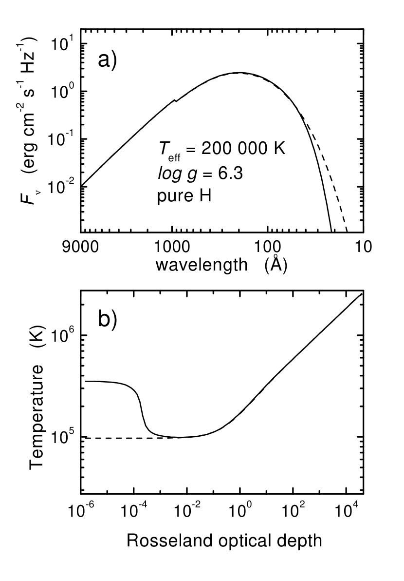
Figure 1: Spectra (a) and temperature structures (b) of a hot DA white dwarf model atmosphere with $T_{\rm eff}=200\,000$ K and $\log\leavevmode\nobreak\ g=6.3$ with (solid line) and without (dashed line) Compton scattering taken into account.

2.2 Method 2

Our second approach adopts the equation of transfer for absorption and scattering presented by Sampson (1959) and Pomraning (1973, see Eqn. (2.167)). The equation of transfer can be expressed in the form

$${\partial^{2}f_{\nu}J_{\nu}\over{\partial\tau_{\nu}^{2}}} = {k_{\nu}\over{k_{\nu}+\sigma_{\nu}}}\,(J_{\nu}-B_{\nu})+$$ (14)

$$+ {\sigma_{\nu}\over{k_{\nu}+\sigma_{\nu}}}\,J_{\nu}\,\int\limits_{0}^{\infty}\Phi(\nu,\nu^{\prime})\,\left(1+{c^{2}\over{2h{\nu^{\prime}}^{3}}}J_{\nu^{\prime}}\right)\,d\nu^{\prime}$$

$$- {\sigma_{\nu}\over{k_{\nu}+\sigma_{\nu}}}\,\left(1+{c^{2}\over{2h\nu^{3}}}J_{\nu}\right)\,\times$$

$$\int\limits_{0}^{\infty}\Phi(\nu,\nu^{\prime})J_{\nu^{\prime}}\,{\left({\nu\over{\nu^{\prime}}}\right)}^{3}\exp\left[-{{h(\nu-{\nu^{\prime}})}\over{kT}}\right]\,d\nu^{\prime}.$$

This transfer equation is written on the monochromatic optical depth scale $d\tau_{\nu}=-(k_{\nu}+\sigma_{\nu})\,\rho\,dz$. The variable $J_{\nu}$ denotes the energy-dependent mean intensity of radiation. The function $\Phi(\nu,\nu^{\prime})$ denotes the zeroth angular moment of the angle-dependent differential cross-section, normalized to unity (see below).

Transformation of the equation of transfer by Pomraning (1973) to the Eq. 14 and the definition of required angular approximations for Compton scattering in a stellar atmosphere was outlined by Madej (1991, 1994) and Madej et al. (2004).

Our equations and theoretical models of Method 2 use detailed differential cross-sections for Compton scattering, $\sigma(\nu\to\nu^{\prime},\@vec{n}\cdot\@vec{n^{\prime}})$, which were taken from Guilbert (1981). Cross-sections correspond to scattering in a gas of free electrons with relativistic thermal velocities, and they are also completely valid at low temperatures. Differential cross-sections were then integrated numerically to obtain large grids of Compton scattering opacity coefficients $\sigma_{\nu}$

$$\sigma_{\nu}=\oint_{\omega^{\prime}}\frac{d\omega^{\prime}}{4\pi}\int^{\infty}_{0}d\nu^{\prime}\,\sigma(\nu\to\nu^{\prime},\@vec{n}\cdot\@vec{n^{\prime}})\,,$$ (15)

and grids of angle-averaged Compton scattering redistribution functions $\Phi(\nu,\nu^{\prime})$

$$\Phi(\nu,\nu^{\prime})={1\over{\sigma_{\nu}}}\oint_{\omega^{\prime}}\frac{d\omega^{\prime}}{4\pi}\,\sigma(\nu\to\nu^{\prime},\@vec{n}\cdot\@vec{n^{\prime}})\,.$$ (16)

The scattering frequency redistribution function was introduced by Pomraning (1973)—see Eqn. (7.95) of his book—and it represents the normalized probability density of scattering from a given frequency $\nu$ to the outgoing frequency $\nu^{\prime}$.

Note that Eq. 14 also includes stimulated scattering terms, $1+(c^{2}/2h\nu^{3})\,J_{\nu}$, which ensure the physically correct description of Compton scattering. The actual equations and calculations used here strongly differ from those in Madej (1998). The physics of Compton scattering used here is also fundamentally different to Method 1. Note, that the latter method and that of Madej (1998) employ the well-known Kompaneets diffusion approximation to Compton scattering kernels. The apparent difference between Methods 1 and 2 is that they use either the differential Kompaneets kernel (Method 1) or kernels given by integrals over the detailed Compton scattering profiles (Method 2).

The equation of radiative equilibrium (the energy balance equation) requires that

$$\int^{\infty}_{0}H_{\nu}\,d\nu=\frac{\sigma_{R}T_{\rm eff}^{4}}{4\pi}\,.$$ (17)

The above condition is fulfilled in a hot stellar atmosphere, where energy transport by convective motions can be neglected.

Computing derivatives of both sides of Eqn. 17 and using the equation of transfer, Eqn. 14, one can obtain the alternative energy balance equation

$$\int\limits_{0}^{\infty}k_{\nu}\,(J_{\nu}\,-B_{\nu})\,d\nu+\int\limits_{0}^{\infty}\sigma_{\nu}J_{\nu}d\nu\int\limits_{0}^{\infty}\Phi(\nu,\nu^{\prime})\,\left(1+{c^{2}\over{2h{\nu^{\prime}}^{3}}}J_{\nu^{\prime}}\right)\, d\nu^{\prime}\,$$

$$\hskip-199.16928pt-\int\limits_{0}^{\infty}\sigma_{\nu}\left(1+{c^{2}\over{2h\nu^{3}}}J_{\nu}\right)\,d\nu$$

$$\int\limits_{0}^{\infty}J_{\nu^{\prime}}\,\Phi(\nu,\nu^{\prime})\,{\left({\nu\over{\nu^{\prime}}}\right)}^{3}\exp\left[-{{h(\nu-{\nu^{\prime}})}\over{kT}}\right]\,d\nu^{\prime}=0\,,$$ (18)

which can be compared with its analog, the Eqn. 5 of Method 1.

The computer code atm21 used for the model calculations was described in detail in Madej & Rózańska (2000) and Madej et al. (2004). The structure of the code is based on the partial linearization scheme by Mihalas (1978), in which corrections of temperature $\Delta T$ and the function $\Delta\Phi$ are built into the equation of transfer. The high numerical accuracy and very good convergence properties of the atm21 code are vital for the present paper, and allowed us to compute accurate spectra for atmospheric parameters appropriate for the white dwarfs HZ 43 and Sirius B using Method 2, outlined above. These calculations supersede less accurate X-ray spectra of HZ 43 which were presented in the earlier paper (Madej, 1998).

For the present research, the atm21 code included numerous bound-free LTE opacities of neutral hydrogen and free-free opacity of ionized hydrogen, which always remains in LTE. No hydrogen lines were included in the actual computations. In each temperature iteration the code solves the equation of hydrostatic equilibrium to obtain stratifications of gas pressure $P_{g}$ and density $\rho$ in the model atmosphere. After that the atm21 code solves the set of coupled equations of radiative transfer with implicit temperature corrections and finds the stratification of $\Delta T$ in the model atmosphere. The equation of radiative transfer was solved using the Feautrier method and the technique of variable Eddington factors (Mihalas, 1978). Boundary conditions along the $\tau_{\nu}$ axis were the same as in Method 1. Explicit expressions for the temperature corrections, $\Delta T$, can be found, e.g., in Madej et al. (2004).

3 Computations and Results

Using our two independent methods, we investigated the effects of Compton scattering on the emergent spectra of three pure H white dwarf models. These were: models appropriate for the well-known DA white dwarfs Sirius B (assuming $T_{\rm eff}=24\,700$ K, $\log\leavevmode\nobreak\ g=8.6$) and HZ 43 ($T_{\rm eff}=50\,000$ K, $\log\leavevmode\nobreak\ g=8.0$), together with a significantly hotter model with $T_{\rm eff}=1\cdot 10^{5}$ K and $\log\leavevmode\nobreak\ g=6$ and $8$. These models cover the effective temperature range relevant to pure H DA atmospheres and specifically address the question of whether Compton scattering might be relevant to the X-ray bright DA white dwarfs Sirius B and HZ 43 that are central to the low-energy calibration of Chandra (Pease et al., 2003).

The results of our calculations from both methods are presented in Figures 2-5. In Fig. 2a the spectra of the model atmosphere for the DA white dwarf HZ 43 ($T_{\rm eff}=50\,000$ K, $\log\leavevmode\nobreak\ g=8.0$) computed using Method 1 with (solid line) and without (dashed line) Compton effects are shown. We also calculated a non-LTE model atmosphere for HZ 43 using the Tübingen Model Atmosphere Package (TMAP) (Werner et al., 2003) and computed the radiation transfer equation (3) with Compton scattering using this non-LTE model atmosphere structure. The corresponding spectra are shown in Fig. 2a by the dotted line and by open circles.

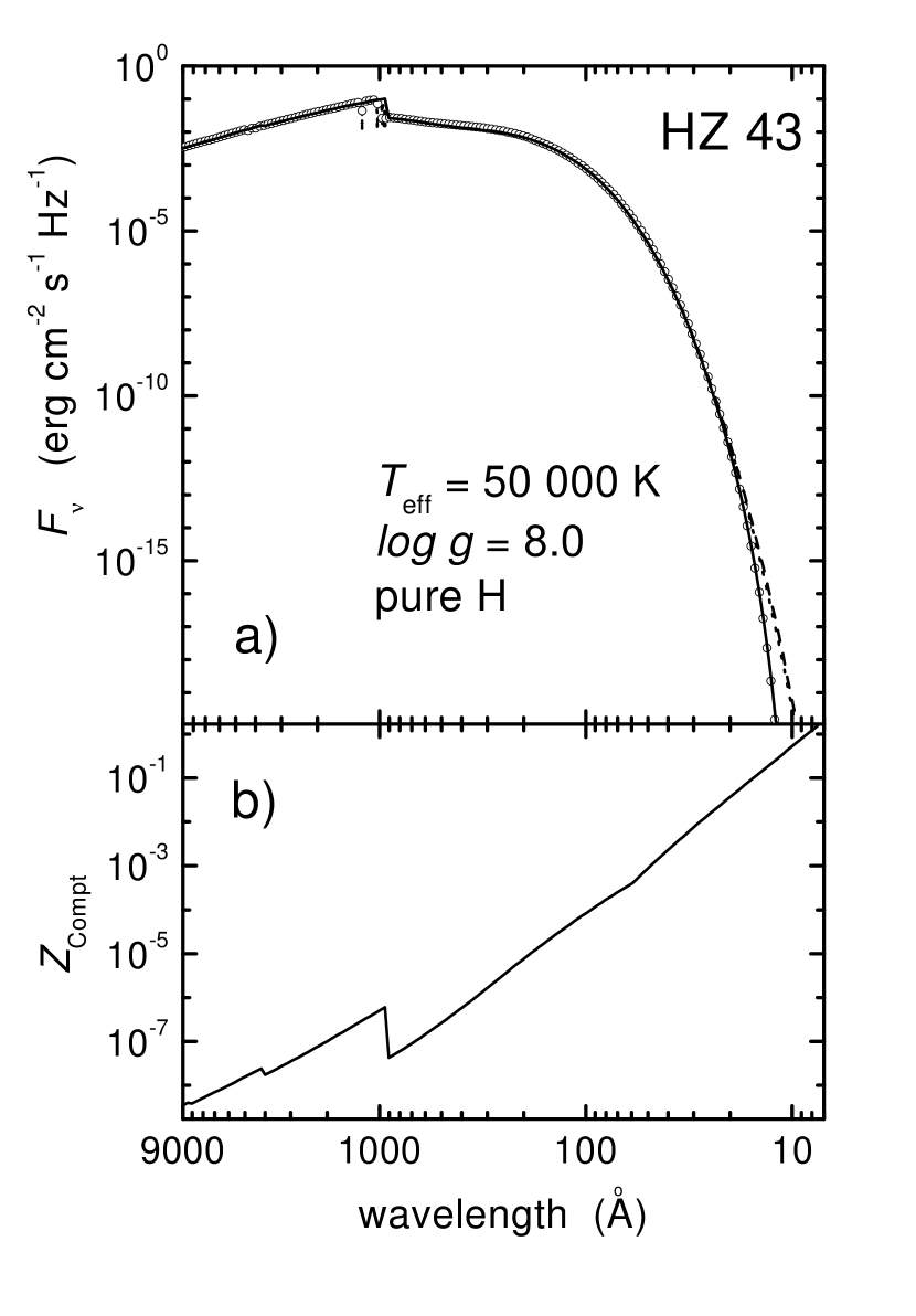
Figure 2: Spectra (a) of the DA white dwarf HZ 43 model atmosphere with (solid line) and without (dashed line) Compton scattering using Method 1. Also shown are the spectra of the non-LTE model atmosphere (dotted line) and the spectra of non-LTE model atmosphere with Compton scattering (open circles). Run (b) of Comptonisation parameter $Z_{\rm Compt}$ with wavelength (see Eqn. 19).

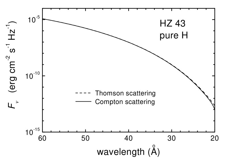
Figure 3: Emergent X-ray spectra for a pure hydrogen model atmosphere appropriate for the parameters of HZ 43 computed for classical Thomson scattering (dashed) and Compton scattering (solid) using Method 2 (the method of Madej et al. 2004).

Calculations using Method 2 in LTE are illustrated in Fig. 3. The differences between Compton and Thomson models in these calculations are very similar to the differences found in Method 1 in Fig. 2a, and are significant only at wavelengths $<25$ Å. The flux in the models with Compton scattering (Method 1) is smaller than the flux in the model without Compton scattering by 0.5% at 50 Å, 1.3% at 40 Å, 7% at 30 Å, and 40% at 20 Å. Similarly, model computations performed with Method 2 yield the following differences for HZ 43: 0.5% at 50 Å, 1.4 % at 40 Å, 5% at 30 Å, and 56% at 20 Å.

These results can be understood more clearly if we consider the Comptonisation parameter $Z_{\rm Compt}$:

$$Z_{\rm Compt}=\frac{h\nu}{m_{\rm e}c^{2}}\max((\tau_{\rm e}^{*})^{2},\tau_{\rm e}^{*}),$$ (19)

where $h\nu/m_{\rm e}c^{2}$ is the relative photon energy lost during one scattering event off a cool electron, $\max((\tau_{\rm e}^{*})^{2},\tau_{\rm e}^{*})$ is the number of scattering events the photon undergoes before escaping, $\tau_{\rm e}^{*}$ is the Thomson optical depth, corresponding to the depth where escaping photons of a given frequency are created. The Comptonisation parameter is, then, a representation of the influence of Compton down-scattering on the emergent spectrum: significant Compton effects are expected if the Comptonisation parameter approaches unity (Rybicki & Lightman, 1979). In Fig.2b the dependence of $Z_{\rm Compt}$ on the wavelength is shown. It is clear that the Comptonisation parameter is very small down to 25 Å, and this is indeed reflected in the emergent spectrum.

Similar results were obtained for the DA white dwarf Sirius B (assuming $T_{\rm eff}=24\,700$ K, $\log\leavevmode\nobreak\ g=8.6$). The corresponding spectra and the Comptonisation parameter are shown in Fig. 4. The effective temperature of this star is smaller, and the surface gravity is larger, therefore, Compton scattering is even less significant than for HZ 43. We also calculated a non-LTE model atmosphere for Sirius B using the TMAP and computed the radiation transfer equation (3) with Compton scattering using this non-LTE model atmosphere structure, as for HZ 43. The corresponding spectra are shown in Fig. 4a by the dotted line and by open circles. Compton scattering changes only very slightly the emergent spectrum at wavelengths below 20 Å.

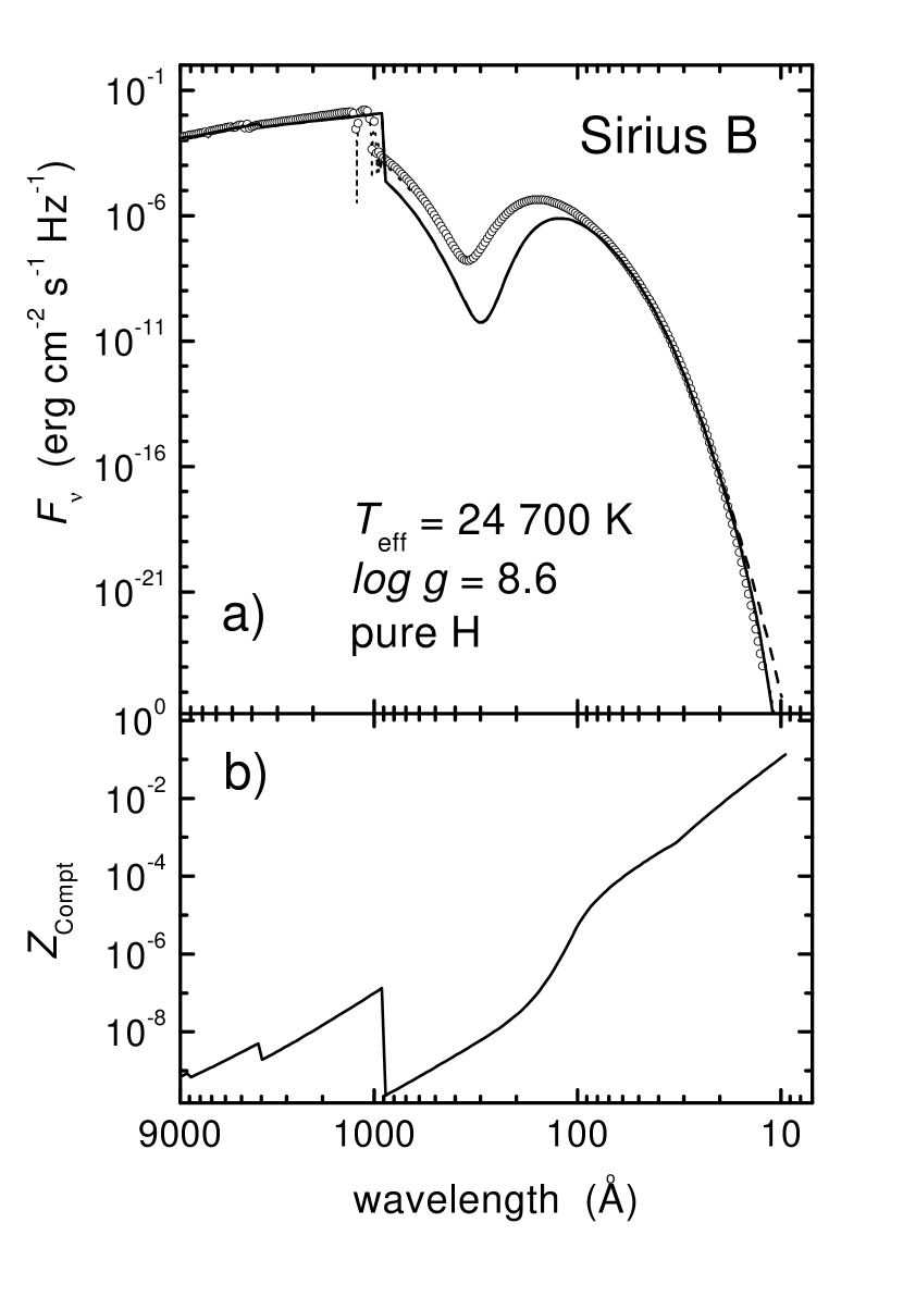
Figure 4: The same as Fig. 2 but here for the DA white dwarf Sirius B LTE model atmosphere. The dotted line lies everywhere under the open circules (except for hydrogen lines).

In the Fig. 5 we present the spectra of the hot DA white dwarfs model atmospheres ($T_{\rm eff}=100\,000$ K, $\log\leavevmode\nobreak\ g=6$ and $8$) with and without Compton scattering. It is obvious that Compton effects are more significant for these hot DA models (especially with low surface gravity) than for Sirius B and HZ 43, but visible effects still do not occur for wavelengths $>50$ Å. Of course, $\log\leavevmode\nobreak\ g=6$ is not a so realistic value for white dwarfs, but we calculate this model to demonstrate the dependence of the Compton effect on the surface gravity.

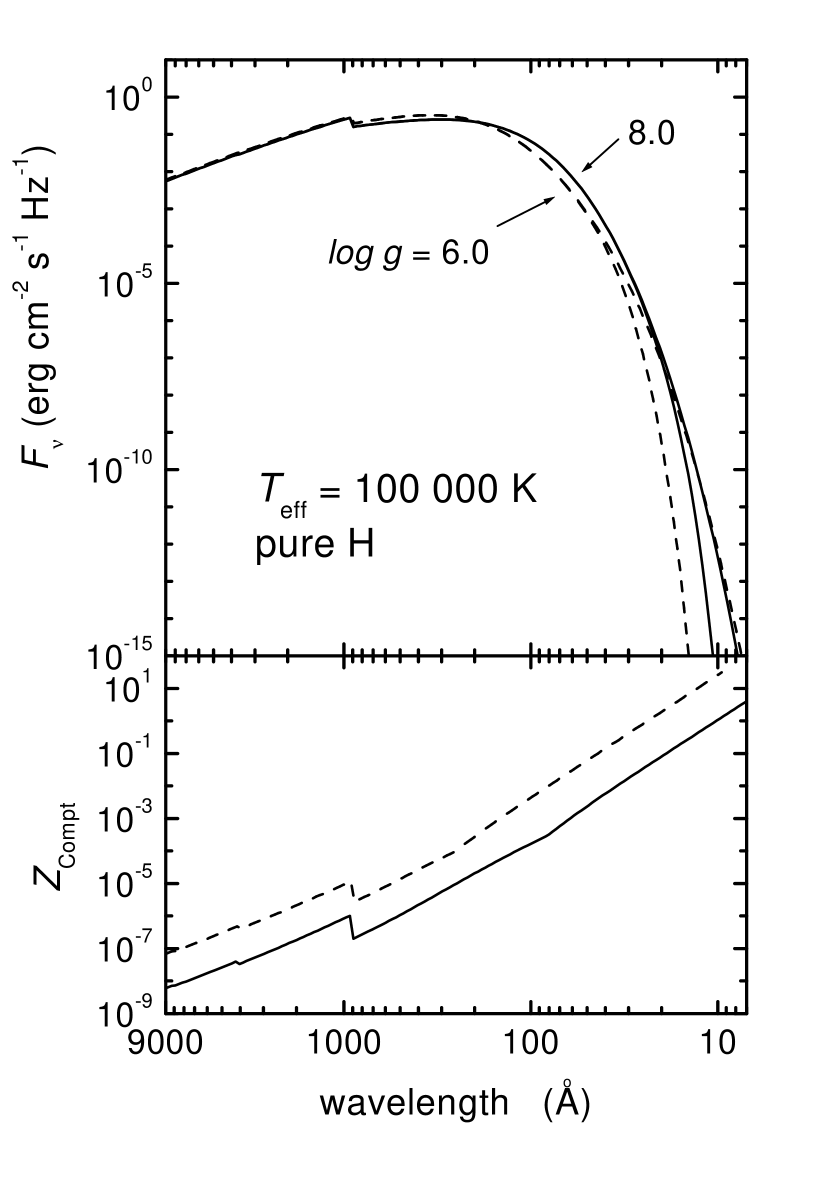
Figure 5: Spectra (a) of the DA white dwarf $T_{\rm eff}=100\,000$ K model atmospheres with and without Compton scattering. Solid lines correspond to model with $\log\leavevmode\nobreak\ g=8.0$, and dashed lines correspond to model with $\log\leavevmode\nobreak\ g=6.0$. Softer high energy tails correspond to models with Compton effect. Run (b) of Comptonisation parameter $Z_{\rm Compt}$ with wavelength.

4 Discussion

The differences we find here between emergent spectra computed using Thomson and Compton scattering are essentially negligible for practical purposes. Such differences are in fact much smaller than the predicted spectral uncertainties resulting from uncertainties in the current knowledge of the fundamental parameters of DA white dwarfs - even the best known examples such as HZ 43 and Sirius B. The spectrum in this Wien tail region is especially sensitive to uncertainties in the effective temperature.

Comparison of the calculations presented here using both Methods 1 and 2 with the earlier work of Madej (1998) do, however, reveal some significant differences. For HZ 43, Fig. 3 of Madej (1998) suggests a large X-ray flux deficit due to Compton scattering of photons to longer wavelengths, with a precipitous decline in emergent flux at $\sim 40$ Å. However, our Figs. 2 and 3 illustrate much smaller effects.

A careful examination of the Madej (1998) computer code performed by one of us (JM) has shown that the earlier code (which used Kompaneets scattering terms) could strongly exaggerate effects of Compton scattering in cases when they were of only marginal significance. This is the case for the X-ray spectrum of HZ 43. The effect was caused by an approximation adopted in the solution of the transfer equation that was quite valid for the study of X-ray burst sources, for which the code was primarily developed, but which became marginally inaccurate for the case of hot DA white dwarf atmospheres. This problem has been solved by the very stable algorithm of the new code (see Method 2), described in Madej & Rózańska (2000).

One should note that the differences between this work and that of Madej (1998) are not related to the numerical approaches adopted for Compton scattering. Both the Kompaneets diffusion approximation (Method 1) and the Compton scattering terms of the integral form (Method 2) satisfactorily describe effects of Compton scattering in X-ray spectra of hot white dwarf stars. The results of the work presented here using both methods supersede those of Madej (1998).

At the higher effective temperatures represented by the $T_{\rm eff}=100\,000$ K models, the emergent spectra for Thomson and Compton scattering begin to diverge at $\sim 50$ Å for the $\log g=6$ model, and the effects are much larger toward shorter wavelengths than for the higher gravity $\log g=8$ case. It is of course questionable as to whether any white dwarfs with pure H atmospheres exist with such high effective temperatures, since in hotter stars radiative levitation tends to enrich the atmosphere with metals. In atmospheres with significant metal abundances the electron scattering opacity is insignificant compared with that due to metals, and Compton redistribution effects are rendered irrelevant.

Our calculations show that even in the hottest pure H atmospheres it is highly unlikely that future X-ray observations will be sufficiently sensitive to discern the Compton redistribution effects. Again, uncertainties in model parameters such as effective temperature and surface gravity, and abundances of He and trace elements, together with uncertainties in parameters entering into the modeling calculations themselves will dominate. Even for models normalised to the same flux at UV wavelengths a 1% error in $T_{\rm eff}$ will induces a 20% flux error at 75Å.

5 Conclusions

New calculations using two independent, rigorous numerical methods confirm that the effects of Compton energy redistribution in photon-electron scattering events are completely negligible for the interpretation of X-ray spectra of DA white dwarfs such as Sirius B and HZ 43. Differences between emergent spectra of Compton and Thomson cases are in fact much smaller than the predicted spectral uncertainties resulting from uncertainties in the current knowledge of the fundamental parameters of stars such as HZ 43. We have found that differences between Compton effects predicted here for HZ 43 and the calculations of Madej (1998) are caused by approximations used in the solution of the transfer equation in the former work; the results presented here supersede the earlier ones. We conclude that current non-LTE model atmosphere spectra of hot DA white dwarfs neglecting Compton scattering can be safely used for the calibration low energy detectors of X-ray observatories for the foreseeable future.