Reionisation scenarios and the temperature of the IGM

Abstract

We examine the temperature structure of the IGM due to the passage of individual ionisation fronts using a radiative transfer (RT) code coupled to a particle-mesh (PM) $N$-body code. Multiple simulations were performed with different spectra of ionising radiation: a power law ($\propto\nu^{-0.5}$), miniquasar, starburst, and a time-varying spectrum that evolves from a starburst spectrum to a power law. The RT is sufficiently resolved in time and space to correctly model both the ionisation state and the temperature across the ionisation front. We find the post-ionisation temperature of the reionised intergalactic medium (IGM) is sensitive to the spectrum of the source of ionising radiation, which may be used to place strong constraints on the nature of the sources of reionisation. Radiative transfer effects also produce large fluctuations in the He $\rm\scriptstyle II$ to H $\rm\scriptstyle I$ number density ratio $\eta$. The spread in values is smaller than measured, except for the time-varying spectrum. For this case, the spread evolves as the spectral nature of the ionising background changes. Large values for $\eta$ are found in partially ionised He $\rm\scriptstyle II$ as the power-law spectrum begins to dominate the starburst, suggesting that the large $\eta$ values measured may be indicating the onset of the He $\rm\scriptstyle II$ reionisation epoch.

1 Introduction

The process by which the Universe was reionised is one of the premier unsolved questions in cosmology. Measurements of the Ly$\alpha$ optical depth of the Intergalactic Medium (IGM) along Quasi-Stellar Object (QSO) lines-of-sight require the IGM to have been reionised by $z\ga 6$ (Becker & et al, 2001), consistent with recent measurements of the Cosmic Microwave Background (CMB) by the Wilkinson Microwave Anisotropy Probe (WMAP), although a higher redshift of $z\sim 11$ is preferred, with a 2-$\sigma$ upper limit of $z\la 17$ (Spergel & et al, 2007). The sources of the reionisation are currently unknown. The most recent estimates of the numbers of high redshift QSOs suggest QSOs are too few to have ionised the H $\rm\scriptstyle I$ prior to $z\approx 4$, without an upturn in the QSO luminosity function at the faint end (Meiksin, 2005). While an adequate supply of ionising photons is likely produced within young, star-forming galaxies, it has yet to be conclusively demonstrated that the ionising photons are able to escape in sufficient numbers to meet the requirements for reionisation (Fernández-Soto et al., 2003; Malkan et al., 2003). Other, more speculative, possibilities include pockets of Population III stars (e.g., in young galaxies or star clusters)(Choudhury & Ferrara, 2006) or miniquasars (Madau et al., 2004).

The post-ionisation IGM temperature may provide a clue to the nature of the reionisation sources. Low density regions retain a memory of the post-ionisation temperature (Meiksin, 1994; Miralda-Escude & Rees, 1994). Evidence for temperatures in excess of the optically thin predictions at high redshifts ($z>3$) is provided by the widths of the low column density Ly$\alpha$ forest absorbers (Meiksin et al., 2001) which are expected to reside in the underdense regions comprising most of the volume of the Universe (Zhang et al., 1998).

In the past few years, several groups have implemented numerical radiative transfer schemes to solve for the reionisation of the IGM (Abel et al., 1999; Gnedin & Abel, 2001; Nakamoto et al., 2001; Razoumov et al., 2002; Ciardi et al., 2003; Iliev et al., 2006; Whalen & Norman, 2006). Most of the modelling of IGM reionisation has focused on the propagation of ionisation fronts (I-fronts), with less emphasis given to the accurate computation of post-ionisation temperatures (Iliev et al., 2006), as the required calculations are much more computationally demanding (Bolton et al., 2004; Bolton & Haehnelt, 2007). Crucial to accurate temperatures is the resolution of the ionisation fronts, particularly for hard spectrum sources like young galaxies or Active Galactic Nuclei (AGN). Early estimates of the post-ionisation IGM temperature were made assuming optically thin gas. Accounting for radiative transfer within the ionisation fronts produces much higher temperatures.

In this paper, we focus on the thermal properties of the post-ionised IGM. We investigate the role played by the spectral shape of the dominant ionising sources on the temperature of the post-ionised IGM, considering both soft sources like galaxies and hard like QSOs. Rather than performing a full reionisation simulation with multiple sources, which is still beyond the current resources of numerical computations, we limit the computations to a single ionisation front sweeping across the box, as would occur prior to the time of the complete overlap of ionisation fronts. Although this approximation will not allow us to compute precise values for the ionisation fractions of hydrogen and helium for comparison with measurements, as these levels will be reset by the subsequent total photoionisation rates after I-fronts overlap, it does permit a quantitative evaluation of the temperature structure after complete reionisation. This is because, once ionised, the temperature is insensitive to the total intensity or shape of the ionising background (Meiksin, 1994; Hui & Gnedin, 1997), which will readjust both due to the overlapping of I-fronts and the evolution of the sources and photoelectric optical depth of the IGM.

The simulations are performed with a radiative transfer code coupled to an $N$-body code to model the evolution of the IGM. In §2 the algorithm and the numerical code are described. The details of the simulation volume and sources are given in §3. Results of the simulations are provided in §4 and discussed in §5.

2 Method

The simulation code, PMRT_mpi, is the merger of a Lagrangian particle-mesh (PM) code (Meiksin et al., 1999), and a grid-based radiative transfer (RT) code which are modularly independent. We perform the RT on the evolving gas density field, as computed by the PM code. Full hydrodynamical simulations have shown that the gas density closely traces the dark matter density down to the Jeans scale ($\sim 100$ kpc) (Cen et al., 1994; Zhang et al., 1998). Statistical comparisons between the resulting Ly$\alpha$ forest properties show good agreement at the 10 per cent level (Meiksin & White, 2001; Viel et al., 2002).

The gas density is taken as a constant fraction ($\Omega_{b}/\Omega_{m}$) of the total density. This is a fair approximation since baryons trace dark matter (Zhang et al., 1998) and in simulations with gas, the gas to dark matter ratio doesn’t vary more than a factor of 30 percent over the over density range $\delta=0.1$ to 1000 (Tittley & Couchman, 2000). The I-fronts propagate much faster than the sound speed, so that the pressure-response of the gas has only a small effect on the reionisation. The PM code evolves the density field assuming all mass is collisionless, interacting only gravitationally.

The density field is determined from the particle distribution by griding the particles on to a mesh. To avoid low-count artefacts in low-density regions while not sacrificing information in dense regions, the density field is separated into two fields, $\rho(\mathop{\bf r\,}\nolimits)=\rho_{lo}(\mathop{\bf r\,}\nolimits)+\rho_{hi}(\mathop{\bf r\,}\nolimits)$, and the low-density field, $\rho_{lo}(\mathop{\bf r\,}\nolimits)$, is convolved with a Gaussian of radius two grid cells. A threshold cell count ($N_{thresh}=5$ for these simulations) discriminates $\rho_{lo}(\mathop{\bf r\,}\nolimits)$ from $\rho_{hi}(\mathop{\bf r\,}\nolimits)$. In dense regions, $\rho_{lo}(\mathop{\bf r\,}\nolimits)=N_{thresh}$ and $\rho_{hi}(\mathop{\bf r\,}\nolimits)=\rho(\mathop{\bf r\,}\nolimits)-N_{thresh}$, while in low-density regions, $\rho_{lo}(\mathop{\bf r\,}\nolimits)=\rho(\mathop{\bf r\,}\nolimits)$. The smoothed field is then $\rho^{\prime}(\mathop{\bf r\,}\nolimits)=\rho_{lo}(\mathop{\bf r\,}\nolimits)\otimes g(\mathop{\bf r\,}\nolimits)+\rho_{hi}(\mathop{\bf r\,}\nolimits)$ where $g$ is the Gaussian smoothing kernel.

2.1 Radiative transfer

The RT code uses a probabilistic method which is based on the photon-conserving algorithm of Abel et al. (1999), extended to include helium by Bolton et al. (2004) who applied the RT algorithm to a density field frozen in the comoving frame. For convenience, we provide details of the RT code here.

The rates of change of the ionisation-state populations due to ionisations and recombinations are given by:

$$\dot{n}_{\rm H\hskip 1.0pt\scriptscriptstyle I} = n_{e}n_{\rm H\hskip 1.0pt\scriptscriptstyle II}\alpha_{\rm H\hskip 1.0pt\scriptscriptstyle II}-n_{\rm H\hskip 1.0pt\scriptscriptstyle I}\Gamma_{\rm H\hskip 1.0pt\scriptscriptstyle I}$$ (1)

$$\dot{n}_{\rm H\hskip 1.0pt\scriptscriptstyle II} = -\dot{n}_{\rm H\hskip 1.0pt\scriptscriptstyle I}$$

$$\dot{n}_{\rm He\hskip 1.0pt\scriptscriptstyle I} = n_{e}n_{\rm He\hskip 1.0pt\scriptscriptstyle II}\alpha_{\rm He\hskip 1.0pt\scriptscriptstyle II}-n_{\rm He\hskip 1.0pt\scriptscriptstyle I}\Gamma_{\rm He\hskip 1.0pt\scriptscriptstyle I}$$

$$\dot{n}_{\rm He\hskip 1.0pt\scriptscriptstyle II} = -\dot{n}_{\rm He\hskip 1.0pt\scriptscriptstyle I}-\dot{n}_{\rm He\hskip 1.0pt\scriptscriptstyle III}$$

$$\dot{n}_{\rm He\hskip 1.0pt\scriptscriptstyle III} = n_{\rm He\hskip 1.0pt\scriptscriptstyle II}\Gamma_{\rm He\hskip 1.0pt\scriptscriptstyle II}-n_{e}n_{\rm He\hskip 1.0pt\scriptscriptstyle III}\alpha_{\rm He\hskip 1.0pt\scriptscriptstyle III}$$

where $\alpha_{i}$ is the recombination coefficient from species $i$ and $\Gamma_{i}$ is the photoionsation rate. Number-density changes, $\dot{n}_{i}$, due to cosmological evolution are accounted for by carrying only the ionisation fractions ($f_{\rm H\hskip 1.0pt\scriptscriptstyle I}=n_{\rm H\hskip 1.0pt\scriptscriptstyle I}/n_{\rm H}$ and similar for helium fraction $f_{\rm He\hskip 1.0pt\scriptscriptstyle I}$, $f_{\rm He\hskip 1.0pt\scriptscriptstyle II}$, and $f_{\rm He\hskip 1.0pt\scriptscriptstyle III}$) between PM iterations.

Table 1: Recombination ($\alpha_{i}$ [$\mathop{\rm m\,}\nolimits^{3}\mathop{\rm s\,}\nolimits^{-1}$]) and recombination cooling ($\beta_{i}$ [$\mathop{\rm J\,}\nolimits\mathop{\rm m\,}\nolimits^{3}\mathop{\rm s\,}\nolimits^{-1}$]) coefficients.

$\alpha_{\rm H\hskip 1.0pt\scriptscriptstyle II}$	$2.065\times 10^{-17}T^{-{\mbox{\scriptsize${}^{{1}\!}/_{\!{2}}$}}}\left(6.414-\frac{1}{2}\ln\,T+8.68\times 10^{-3}T^{\mbox{\scriptsize${}^{{1}\!}/_{\!{3}}$}}\right)$
$\alpha_{\rm He\hskip 1.0pt\scriptscriptstyle II}$	$3.294\times 10^{-17}\left\{\left(\frac{T}{15.54}\right)^{\mbox{\scriptsize${}^{{1}\!}/_{\!{2}}$}}\left[1+\left(\frac{T}{15.54}\right)^{\mbox{\scriptsize${}^{{1}\!}/_{\!{2}}$}}\right]^{0.309}\left[1+\left(\frac{T}{3.676\times 10^{7}}\right)^{\mbox{\scriptsize${}^{{1}\!}/_{\!{2}}$}}\right]^{1.691}\right\}^{-1}+1.9\times 10^{-9}\left(1+0.3e^{\frac{-9.4\times 10^{4}}{T}}\right)e^{\frac{-4.7\times 10^{5}}{T}}T^{-\mbox{\scriptsize${}^{{3}\!}/_{\!{2}}$}}$
$\alpha_{\rm He\hskip 1.0pt\scriptscriptstyle III}$	$8.260\times 10^{-17}T^{-{\mbox{\scriptsize${}^{{1}\!}/_{\!{2}}$}}}\left(7.107-\frac{1}{2}\ln\,T+5.47\times 10^{-3}T^{\mbox{\scriptsize${}^{{1}\!}/_{\!{3}}$}}\right)$
$\beta_{\rm H\hskip 1.0pt\scriptscriptstyle II}$	$2.851\times 10^{-40}T^{{\mbox{\scriptsize${}^{{1}\!}/_{\!{2}}$}}}\left(5.914-\frac{1}{2}\ln\,T+0.01184T^{{\mbox{\scriptsize${}^{{1}\!}/_{\!{3}}$}}}\right)$
$\beta_{\rm He\hskip 1.0pt\scriptscriptstyle II}$	$1.55\times 10^{-39}T^{0.3647}+1.24\times 10^{-26}\left(1+0.3e^{\frac{-9.4\times 10^{4}}{T}}\right)e^{\frac{-4.7\times 10^{5}}{T}}T^{-\mbox{\scriptsize${}^{{3}\!}/_{\!{2}}$}}$
$\beta_{\rm He\hskip 1.0pt\scriptscriptstyle III}$	$1.140\times 10^{-39}T^{\mbox{\scriptsize${}^{{1}\!}/_{\!{2}}$}}\left(6.607-\frac{1}{2}\ln\,T+7.459\times 10^{-3}T^{\mbox{\scriptsize${}^{{1}\!}/_{\!{3}}$}}\right)$

The forms for the recombination coefficients $\alpha_{\rm H\hskip 1.0pt\scriptscriptstyle II}(T)$ and $\alpha_{\rm He\hskip 1.0pt\scriptscriptstyle III}(T)$ are derived from the generalised hydrogenic case A form given in Seaton (1959). For $\alpha_{\rm He\hskip 1.0pt\scriptscriptstyle II}(T)$, the radiative term is from Verner & Ferland (1996) while the dielectronic term is adopted from Aldrovandi & Pequignot (1973). The recombination coefficients are provided in Table LABEL:table.RecombCoef.

Table 2: Ionisation cross-section parameters used in Eq. 6.

	$\sigma_{T}[\mathop{\rm m\,}\nolimits^{2}]$	$\nu_{T}$ [Hz]	$\beta$	$\mathop{\rm s\,}\nolimits$
$\sigma_{\rm H\hskip 1.0pt\scriptscriptstyle I}$	$6.30\times 10^{-22}$	$3.282\times 10^{15}$	1.34	2.99
$\sigma_{\rm He\hskip 1.0pt\scriptscriptstyle I}$	$7.83\times 10^{-22}$	$5.933\times 10^{15}$	1.66	2.05
$\sigma_{\rm He\hskip 1.0pt\scriptscriptstyle II}$	$1.58\times 10^{-22}$	$1.313\times 10^{16}$	1.34	2.99

The photoionisation rate per particle, $\Gamma$, for each species is dependent on the local mean intensity of radiation, $J_{\nu}$, and the ionisation cross section, $\sigma$, for the species by

$$\Gamma=4\pi\int_{\nu_{T}}^{\infty}\frac{J_{\nu}}{h\nu}\sigma_{\nu}d\nu$$ (2)

where $\nu_{T}$ is the threshold frequency for ionisation, which differs for each species. In the plane wave approximation used here, the local mean intensity is simply the radiation field incident on the volume attenuated by the cumulative optical depth,

$$4\pi J_{\nu}=\frac{L_{\nu}}{4\pi R_{0}^{2}}e^{-\tau_{\nu}}$$ (3)

where $L_{\nu}$ is the luminosity of the source per frequency, $R_{0}$ is the distance of the source from the volume, and $\tau_{\nu}$ is the cumulative optical depth which, at distance R from the source, is:

$$\tau_{\nu}(R)=\sigma_{\rm H\hskip 1.0pt\scriptscriptstyle I}N_{\rm H\hskip 1.0pt\scriptscriptstyle I}+\sigma_{\rm He\hskip 1.0pt\scriptscriptstyle I}N_{\rm He\hskip 1.0pt\scriptscriptstyle I}+\sigma_{\rm He\hskip 1.0pt\scriptscriptstyle II}N_{\rm He\hskip 1.0pt\scriptscriptstyle II}$$ (4)

where the cumulative column depth from the edge of the box to $R$ is

$$N_{i}(R)=\int_{R_{0}}^{R}n_{i}(r)dr.$$ (5)

The ionisation cross sections are approximated using the form given in Osterbrock (1989),

$$\sigma(\nu)=\sigma_{T}\left[\beta\left(\frac{\nu}{\nu_{T}}\right)^{-s}+(1-\beta)\left(\frac{\nu}{\nu_{T}}\right)^{-s-1}\right].$$ (6)

The parameters for the various species are listed in Table LABEL:table.CrossSection. The reionisation is further restricted by imposing a check on the position of the light front to ensure gas is not ionised too early. Neglecting this effect can lead to an over-estimate of the temperature (Madau et al., 1997).

The equations governing the thermal state of the gas are used in their entropic form. The entropy is parametrized by the function

$$S\equiv\frac{P}{\rho^{\gamma}},$$ (7)

where $P$ is the pressure, $\rho$ is the gas density, and $\gamma=5/3$ is the adiabatic index for a monatomic gas. It follows from Eq. 7 that

$$\dot{S}=(\gamma-1)\rho^{-\gamma}(G-L),$$ (8)

where $G$ and $L$ are the thermal gain and loss functions per volume, and

$$T=\frac{\mu m_{u}}{k}S\rho^{\gamma-1}$$ (9)

where $\mu$ is the mean molecular weight of the gas, $m_{u}$ is an atomic mass unit, and $k$ is the Boltzmann constant.

Heating is provided by the excess energy above the ionisation threshold $h\nu_{T}$ of the ionising photons. For a single species of density $n$,

$$G=4\pi n\int_{\nu_{T}}^{\infty}\frac{J_{\nu}\sigma_{\nu}}{\nu}(\nu-\nu_{T})d\nu.$$ (10)

Since all species contribute, the total heating rate is

$$G=G_{\rm H\hskip 1.0pt\scriptscriptstyle I}+G_{\rm He\hskip 1.0pt\scriptscriptstyle I}+G_{\rm He\hskip 1.0pt\scriptscriptstyle II}.$$ (11)

Cooling is provided by recombinations, collisional excitation of the excited levels in neutral hydrogen, and inverse Compton scattering off cosmic microwave background (CMB) photons. As for heating, all species contribute to cooling, giving the total cooling rate

$$L=L_{\rm H\hskip 1.0pt\scriptscriptstyle II}+L_{\rm He\hskip 1.0pt\scriptscriptstyle II}+L_{\rm He\hskip 1.0pt\scriptscriptstyle III}+L_{eH}+L_{C}.$$ (12)

For a single species, recombinations radiate the electron energy $\sim kT$ as photons at the rate $L_{i}=n_{e}n_{i}\beta_{i}(T)$. From H $\rm\scriptstyle II$ and He $\rm\scriptstyle III$, the recombination cooling coefficients $\beta_{i}(T)$ are, as $\alpha_{i}(T)$, from Seaton (1959). For the He $\rm\scriptstyle II$ radiative term we use the expression in Black (1981) while we combine the approximation $\beta_{\rm He\hskip 1.0pt\scriptscriptstyle II}=3\mathop{\rm ryd\,}\nolimits\alpha_{\rm He\hskip 1.0pt\scriptscriptstyle II}$ (Gould & Thakur, 1970) with the second $\alpha_{\rm He\hskip 1.0pt\scriptscriptstyle II}$ term listed in Table LABEL:table.RecombCoef (Aldrovandi & Pequignot, 1973) for the dielectronic component. The total recombination cooling coefficients are provided in Table LABEL:table.RecombCoef.

For the cooling rate from collisional excitation of H $\rm\scriptstyle I$ we adopt the approximation of Spitzer (1978):

$$L_{eH}=7.3\times 10^{-32}\mathop{\rm J\,}\nolimits\mathop{\rm m\,}\nolimits^{3}\mathop{\rm s\,}\nolimits^{-1}n_{e}n_{\rm H\hskip 1.0pt\scriptscriptstyle I}e^{-118400/T}.$$ (13)

We note that for the temperatures relevant here, cooling losses due to collisional ionisation of hydrogen and collisional excitation and ionisation losses from helium are negligible.

Finally, Compton scattering off CMB photons cools the gas at the rate (Peebles, 1968)

$$L_{C}=\frac{4\sigma_{T}ak}{m_{e}c}n_{e}T^{4}_{CMB}(z)\left[T-T_{CMB}(z)\right],$$ (14)

where $\sigma_{T}$ is the Thomson cross section, $a$ is the radiation density constant, $m_{e}$ is the electron mass, $c$ is the speed of light, and $T_{CMB}$ is the temperature of the microwave background.

In the current implementation, the simulations do not solve for the overlapping of ionisation fronts. Rather, they describe the passage of the first ionisation front across a neutral region. Reionisation will also be affected by the hydrodynamical response of the gas, which is not included here. For low to moderately overdense systems, this has only a moderate effect on the statistical properties of the resulting absorption systems (Meiksin & White, 2001). The hydrodynamical effects are more important for reionisation in denser structures like minihaloes, which can be optically thick at the Lyman edge. Ionisation heating results in an overpressure that drives the gas out of the minihaloes, reducing their densities and making them less effective at slowing the ionisation fronts. Estimates based on the photon consumption rate suggest the role of these systems in slowing the fronts is small (Ciardi et al., 2006).

Another simplification is the absence of diffuse radiation. Radiative recombinations produce a diffuse radiation field throughout the ionised region. Besides the recombination rate, the intensity depends on the amount of clumping of the gas. Estimates range from a boost in the ionisation rate by an additional 10–40 per cent. (Meiksin & Madau, 1993; Haardt & Madau, 1996). After the gas has been ionised, the diffuse field may be accounted for by rescaling the overall radiation level, as the intensity of the radiation field has a negligible effect on the post-ionisation gas temperature. Radiative recombinations will also contribute to the reionisation process itself. The contribution, however, is generally negligible for both hydrogen and helium reionisation (Shapiro & Giroux, 1987; Miralda-Escude & Ostriker, 1990; Meiksin & Madau, 1993; Madau & Meiksin, 1994). An exception is in dense regions in a scenario in which the He $\rm\scriptstyle III$ I-front precedes the H $\rm\scriptstyle II$ I-front. In this case, assuming all photons produced by helium recombinations to the ground state of He $\rm\scriptstyle II$ are locally absorbed by neutral hydrogen atoms, the time to ionise the H $\rm\scriptstyle I$ is

$$t_{\rm He-H} \approx \frac{n_{\rm H}}{5n^{2}_{\rm He}\alpha_{1}^{\rm He}}$$

$$\approx 7.7\times 10^{20}\,{\rm s}\left(\frac{\Omega_{b}h^{2}}{0.020}\right)^{-1}\frac{T_{4}^{0.5}}{1+\delta}(1+z)^{-3},$$

where $\alpha_{1}^{\rm He}$ is the radiative recombination rate to the ground state of He $\rm\scriptstyle II$, $T_{4}$ is the gas temperature in units of $10^{4}$ K, and $\delta$ is the local fractional overdensity. An allowance has also been made for 1.5 additional secondary electrons produced per photoionisation (Shull, 1979). Compared with a Hubble time of $t_{\rm Hub}\approx 14\,{\rm Gyr}(1+z)^{-3/2}$, the ionisation time goes as

$$\frac{t_{\rm He-H}}{t_{\rm Hub}}\approx 640T_{4}^{0.5}\frac{1}{(1+z)^{3/2}(1+\delta)}.$$ (16)

For the range of source turn-on redshifts considered ($8<z<20$), except in very overdense regions, this ratio will be large and hydrogen will remain largely neutral in the interval between helium and hydrogen ionisation. The effect on the temperature will therefore be small, except for very overdense regions. After reionisation, the post-ionisation temperature will be accurately computed even in the highly overdense regions since the temperature is set by the balance between ionisation heating and radiative cooling with no memory of the reionisation history retained (Meiksin, 1994).

Heating by x-rays is automatically included, but not the effect of secondary electrons. The secondary electrons have a negligible effect on the post-ionisation temperature of the gas (Madau et al., 1997). Ahead of the I-front, however, the heating rates will be overestimated by a factor of 2–5, depending on optical depth to the ionising photons (which determines their mean energies) (Shull & van Steenberg, 1985). While the tendency to approach thermal equilibrium reduces the impact of the secondaries on the final temperature, the gas temperature ahead of the I-front is somewhat reduced when the effect of the secondaries is included, as discussed in the next section. Because of the excessive computational expense involved in including the effect of secondaries, we neglect their role on the pre-ionised gas temperatures, but note the effect of secondaries must be included for applications for which the pre-ionised gas temperatures are relevant, as for instance the 21cm signature of the gas at high redshifts (Madau et al., 1997).

None of the above simplifications affects our findings presented in this paper, which concentrates on the post-ionisation thermodynamic properties of the IGM as it relates to the Ly$\alpha$ forest.

2.2 Implementation

To solve the RT equations, we use the probabilistic formulation described in Abel et al. (1999), as extended to multiple species by Bolton et al. (2004). In the probabilistic formulation, the ionisation rate per unit volume due to an incident photon flux per frequency interval, $\mathop{\mathcal{F\,}\,}\nolimits_{\nu}$, is given by

$$n\Gamma=\frac{1}{dr}\int_{\nu_{0}}^{\infty}\mathop{\mathcal{F\,}\,}\nolimits_{\nu}\sigma_{\nu}ndrd\nu.$$ (17)

is approximated as

$$n\Gamma=\frac{1}{dr}\int_{\nu_{0}}^{\infty}\mathop{\mathcal{F\,}\,}\nolimits_{\nu}\left(1-e^{-\tau_{\nu}^{\rm cell}}\right)d\nu$$ (18)

where $\tau_{\nu}^{\rm cell}=\sigma_{\nu}ndr$ is the optical depth of a single cell of width $dr$. This formulation conserves photons and does not lead to excessive ionisations through cells for which $\tau_{\nu}^{\rm cell}>1$. For multiple species, the probability of absorption is spread among the various species and the rate of ionisation must be known for each species. Bolton et al. (2004) describes the split for absorption by H $\rm\scriptstyle I$, He $\rm\scriptstyle I$, and He $\rm\scriptstyle II$. Using their shorthand $p^{i}=e^{-\tau_{\nu}^{i}}$ and $q^{i}=1-e^{-\tau_{\nu}^{i}}$ where the $\tau_{\nu}^{i}$’s are within the cell (as opposed to cumulative), the probabilities of absorption by each species are

$$P_{abs}^{\rm H\hskip 1.0pt\scriptscriptstyle I} = q^{\rm H\hskip 1.0pt\scriptscriptstyle I}p^{\rm He\hskip 1.0pt\scriptscriptstyle I}p^{\rm He\hskip 1.0pt\scriptscriptstyle II}\left(1-e^{-\tau_{\nu}^{\rm cell}}\right)/D$$ (19)

$$P_{abs}^{\rm He\hskip 1.0pt\scriptscriptstyle I} = q^{\rm He\hskip 1.0pt\scriptscriptstyle I}p^{\rm H\hskip 1.0pt\scriptscriptstyle I}p^{\rm He\hskip 1.0pt\scriptscriptstyle II}\left(1-e^{-\tau_{\nu}^{\rm cell}}\right)/D$$ (20)

$$P_{abs}^{\rm He\hskip 1.0pt\scriptscriptstyle II} = q^{\rm He\hskip 1.0pt\scriptscriptstyle II}p^{\rm H\hskip 1.0pt\scriptscriptstyle I}p^{\rm He\hskip 1.0pt\scriptscriptstyle I}\left(1-e^{-\tau_{\nu}^{\rm cell}}\right)/D$$ (21)

with $D=q^{\rm H\hskip 1.0pt\scriptscriptstyle I}p^{\rm He\hskip 1.0pt\scriptscriptstyle I}p^{\rm He\hskip 1.0pt\scriptscriptstyle II}+q^{\rm He\hskip 1.0pt\scriptscriptstyle I}p^{\rm H\hskip 1.0pt\scriptscriptstyle I}p^{\rm He\hskip 1.0pt\scriptscriptstyle II}+q^{\rm He\hskip 1.0pt\scriptscriptstyle II}p^{\rm H\hskip 1.0pt\scriptscriptstyle I}p^{\rm He\hskip 1.0pt\scriptscriptstyle I}$ and $\tau_{\nu}^{\rm cell}=\tau_{\nu}^{\rm H\hskip 1.0pt\scriptscriptstyle I}+\tau_{\nu}^{\rm He\hskip 1.0pt\scriptscriptstyle I}+\tau_{\nu}^{\rm He\hskip 1.0pt\scriptscriptstyle II}$. Equation 17 with $\sigma_{\nu}ndr$ replaced by the $P_{abs}^{i}$’s above is the form implemented in PMRT_mpi. We recast Eq. 10 for each species in a similar manner, to prevent excessive heating.

Both the PM and RT modules were coded in C and parallelised using a message passing interface (MPI) (the PM component previously so (see Meiksin et al., 1999)). MPI is suited to work on distributed memory systems, but works equally well on shared memory systems, albeit not with optimal memory use. The RT module consumes most of the processing time. In the RT module, each LOS is processed by a single computer processor element (PE). In general the time spent by each process on a LOS scales linearly with the resolution along the LOS. In regions of high optical depth, refinements are generated which split the cell into low-optical-depth sections. The number of refinements is a factor in the PE load for a LOS. Load imbalance is possible because the time to process a LOS varies for each LOS, depending on the amount of structure. Load imbalance is alleviated by dynamic (first-come-first-serve) allocation of LOSs to processes. The master node performs the allocation and, consequently, has a significantly lower mean load. The load imbalance with the master node can be reduced by either 1) having one physical processor unit execute both the master and a slave process or 2) using many processor units, so that instead of one-of-few being underused, one-of-many is underused and less time is spent in a non-load-balanced state.

In addition to accurate modelling of the ionisation front, special attention is given to computing accurate post-photoionisation temperatures. This requires sufficient resolution in time and space to correctly model both the ionisation structure of the ionisation front and the temperature across it. This is particularly important when modelling reionisation by sources with hard photons like QSOs. The time step for the radiative transfer is computed, independent of the PM time step, from the cooling, ionisation, recombination, and density-change time scales. The minimum of these time scales is multiplied by a factor of 0.2, found through convergence tests using a uniform medium containing He $\rm\scriptstyle III$ and H $\rm\scriptstyle II$ fronts. Convergence is considered established if the maximum error in the temperature along the LOS (compared with a fiducial run using a factor of 0.1) is less than half a per cent. High spatial resolution at the front is guaranteed by the use of refinements. Any cell in a line of sight (LOS) which is optically thick at the Lyman edge ($\tau>1$) is split into a sufficient number of slices such that $\tau\leq 1$ in each. Convergence tests were similarly used to establish this criterion by comparing with a fiducial run with $\tau\leq 0.05$ per slice. Refinements are normally only generated at the ionisation front.

Integration over frequency of the ionisation (Eq. 2) and heating (Eq. 10) functions is performed using Gauss-Legendre quadrature over the intervals $\nu_{\rm H\hskip 1.0pt\scriptscriptstyle I}$ to $\nu_{\rm He\hskip 1.0pt\scriptscriptstyle I}$ and $\nu_{\rm He\hskip 1.0pt\scriptscriptstyle I}$ to $\nu_{\rm He\hskip 1.0pt\scriptscriptstyle II}$ and Gauss-Laguerre quadrature for the interval $\nu_{\rm He\hskip 1.0pt\scriptscriptstyle II}$ to $\infty$ where $\nu_{i}$ is the ionisation threshold for species $i$. The integration parameters for each of these intervals was tailored to each of the input spectra using convergence tests similar to those described in the previous paragraph.

Of course, the effort required to get the temperatures correct comes at the expense of computer cycles. More than 20000 PE hours were required for the simulations presented here. PMRT_mpi was run in parallel on 8 or 16 PEs drawn from a dedicated cluster of IBM OpenPower 720s or a local cluster of Linux boxes of mixed type.

Validation of the code was accomplished by the use of problems with known solutions and comparison with results produced by an independent code. The analytic solution to the position of a hydrogen ionisation front in a gas of uniform density irradiated by a monochromatic source with photon energy $h\nu=13.6\mathop{\rm eV\,}\nolimits$ (producing no heating) is easily derivable (Iliev et al., 2006, for example). We simulated the passage of an I-front through a gas with $n_{H}=10^{-3}\mathop{\rm cm\,}\nolimits^{-3}$ and $T=10^{4}\mathop{\rm K\,}\nolimits$ ionised by a source producing photons at a rate of $5\times 10^{48}\mathop{\rm s\,}\nolimits^{-1}$ (Test 1 of Iliev et al. (2006)). Over a period of 500 Myr (a few times the recombination time scale), the error in the position of the front was never more than 6 per cent. There is no analytical solution for the gas temperature if irradiated by a non-monochromatic source. However, other simulations exist to which we could compare. One of us (AM) has a radiative transfer code which implements an altogether different method with more physics than we included in PMRT_mpi (Madau et al., 1997). For an $\alpha=0.5$ power-law spectrum ionising a uniform IGM at the mean baryon density, this code (with the effect of secondary electrons switched off) produces post-ionisation gas temperatures of about 18,000 K to 20,000 K at $z=7$. Including the effect of secondary electrons was found to reduce the post-ionisation temperature by about 200 K while the temperature in the gas ahead of the I-front, where helium ionisation releases large numbers of electrons, was reduced by about 1000 K. Our PMRT_mpi code produces post-ionisation gas temperatures of 16,000 K to 23,000 K at this epoch. PMRT_mpi generates the correct ionisation structure and temperatures that agree with both expectations from observations and the result of an independent code. We are confident that given the physics included, the PMRT_mpi code is producing correct results.

3 Simulations

We use PMRT_mpi to simulate the passage of an ionisation front produced by sources with a variety of characteristic spectra. Each I-front computed may be considered to result from a single source with the adopted spectrum, or a group of several neighbouring sources with individual I-fronts that have already overlapped, producing a single advancing I-front through the IGM. Because we treat each line-of-sight separately, the resulting temperature distributions may also be considered as produced by distinct sources, and the resulting temperature statistics an ensemble average over the IGM.

In the following, we describe the sources of ionising radiation (§3.1), estimate the expected characteristic scales of their ionisation fronts at the reionisation epoch (§3.2), describe the volume of space simulated (§3.3) and demonstrate that the results have converged with resolution and are not dominated by cosmic variance (§3.4).

3.1 Sources

Figure 1: Source spectra. The ionisation thresholds for H $\rm\scriptstyle I$, He $\rm\scriptstyle I$, and He $\rm\scriptstyle II$ are indicated.

The source spectra (Fig. 1) were selected to emulate candidate reionisation sources. For the power law, the luminosity is given by $L(\nu)\propto\nu^{-\alpha}$ where $\alpha=0.5$, which corresponds to a hard quasar/QSO/AGN spectrum. The miniquasar spectrum of Madau et al. (2004) is given by $L(x)\propto x^{\mbox{\scriptsize${}^{{1}\!}/_{\!{4}}$}}+8x^{-1}$, $1\leq x\leq 20$; $P(x)\propto 8x^{-1}$, $x\geq 20$ where $x\equiv\nu/\nu_{0}$. The starburst spectrum was produced by PÉGASE (Fioc & Rocca-Volmerange, 1997) for a galaxy 30 Myr after a burst of Pop III (zero metallicity) star formation. The starburst spectrum has an effective spectral index of $\alpha_{\rm eff}=7.4$ just above the Lyman edge. The hybrid model begins with a starburst spectrum, and between $z=5$ and $z=4$ evolves into an $\alpha=0.5$ power law, mimicking a radiation field in which a QSO source dominates.

The order of propagation of the H $\rm\scriptstyle II$ and He $\rm\scriptstyle III$ ionisation fronts is different for the different sources. For a time-invariant spectrum, the He $\rm\scriptstyle III$ I-front precedes the H $\rm\scriptstyle II$ I-front if the spectrum is hard enough, specifically if $\alpha_{\rm eff}<1.8$. The condition is met for both the power-law and miniquasar spectra and, indeed, the He $\rm\scriptstyle II$ was ionised prior to H $\rm\scriptstyle I$ in those simulations. The starburst spectrum certainly fails the condition as it has negligible intensity above $\nu_{\rm He\hskip 1.0pt\scriptscriptstyle II}$. The hybrid spectrum, in which a spectrum dominated by star bursts evolves into one dominated by a power law, leads to the H $\rm\scriptstyle II$ I-front preceding that of He $\rm\scriptstyle III$.

To ensure comparable results, all spectra were normalised to produce an incident hydrogen ionising flux of $1.5\times 10^{7}(1+z)^{2}\mathop{\rm s\,}\nolimits^{-1}\mathop{\rm m\,}\nolimits^{-2}$. This corresponds to a typical flux level driving an ionisation front, as detailed in §3.2. For example, it corresponds to a $L[\nu_{\rm H\hskip 1.0pt\scriptscriptstyle I}]=1.5\times 10^{21}\mathop{\rm W\,}\nolimits\mathop{\rm Hz\,}\nolimits^{-1}$ QSO source with $\alpha=0.5$ at a comoving distance of $5\mathop{\rm Mpc\,}\nolimits$. The flux is adequate to ionise the full simulation volume by $z=3$. We fix the incident flux level to a common level to ensure that differences in the post-reionisation temperature are due to the differences in the incident spectra rather than the time scale for reionisation. We also explore the effect of source turn-on redshift by performing, for each source, simulations with the source turning on at redshifts of $z_{\rm on}=8$, 12, and 20. These were selected to cover the range of redshifts limited by the WMAP and QSO observations. Because of the common incident flux normalisation, these do not correspond to different reionisation scenarios in which the reionisation of the Universe completes at different epochs, as the reionisation histories are nearly identical for $z<8$. It is simply a device that allows us to ensure the results at late times are insensitive to the assumed turn-on redshift of the sources.

The ionising radiation is projected as parallel rays normal to the surface of the simulation volume. This configuration has the computational advantage of allowing all radiative calculations for a given ray to be done in a single column, independent of neighbouring columns. Since no information about the thermal state of the gas is carried with the particles as they move from one cell to another, each column can be interpreted as an individual line of sight which is independent of any other line of sight. We select 256 lines of sight arranged in a plane to assist in visually interpreting the passage of the front while providing enough lines of sight to deal with cosmic variance. The radiation field takes the plane-wave approximation and is not geometrically diluted by $r^{-2}$. A limited number of simulations performed with the radiation field geometrically diluted produced results similar to those without the dilution factor.

Table 3: Identifiers for the various models used in this paper.

	$z_{\rm on}$
Model	8	12	20
Power Law	PL08	PL12	PL20
Miniquasar	MQ08	MQ12	MQ20
Starburst	SB08	SB12	SB20
Hybrid	HY08	HY12	HY20

For brevity, the labels listed in Table LABEL:table.identifiers will be used henceforth to identify the various simulations with their combination of model spectrum and source turn-on redshift.

3.2 Characteristic sizes of ionised regions

A key effect for which radiative transfer is required is the modification of the source spectrum incident on a region by intervening gas, including shadowing by dense knots. The amount of modification depends on the amount and nature of the intervening gas. In this section, we estimate the typical distances expected between a source and the I-front it produces, and show that our simulations match the distances for a wide range of plausible sources. This is important, because the no-overlap approximation we make is only valid provided the I-fronts do not extend further than the characteristic size of an I-front at the time of complete reionisation, when the porosity of the ionised gas in the IGM crosses unity.

At the time of complete reionisation, the mean space density of the sources is the inverse of the characteristic volume of the ionised gas bubbles just before their complete percolation. For any given characteristic luminosity per source, the source space density may be estimated from the total emissivity of all the sources just prior to complete reionisation. We adopt an estimate for the emissivity based on the constraints imposed by the measured IGM Ly$\alpha$ optical depth up to $z\approx 6$ in a $\Lambda$CDM cosmology (Meiksin & White, 2003, 2004; Meiksin, 2005). At $z=6$, the rate of H $\rm\scriptstyle I$ ionising photons per comoving volume was found to be $\dot{n}_{S}\approx 4\times 10^{50}\alpha_{S}^{-1}h{\rm s^{-1}\,Mpc^{-3}}$(Meiksin, 2005), where $\alpha_{S}$ is the spectral index of the ionising sources at the H $\rm\scriptstyle I$ Lyman edge and $h$ is defined by the Hubble parameter ($H_{0}=100h\mathop{\rm km\,}\nolimits\mathop{\rm s\,}\nolimits^{-1}\mathop{\rm Mpc\,}\nolimits^{-1}$, where $H_{0}$ is the present day value of the Hubble parameter). For a source producing ionising photons at the rate $\dot{N}_{\gamma}$, the corresponding volume of ionised gas at the time of overlap is then $V_{I}\approx\dot{N}_{\gamma}/\dot{n}_{S}$. The characteristic comoving size of an I-front at $z=6$ is then (for $h=0.71$),

$$R_{I}\approx\left(\frac{3}{4\pi}\frac{\dot{N}_{\gamma}}{\dot{n}_{S}}\right)^{1/3}\approx 9\alpha_{S}^{1/3}\left(\frac{\dot{N}_{\gamma}}{10^{54}\,{\rm s^{-1}}}\right)^{1/3}\,{\rm Mpc}.$$ (22)

This scale agrees with estimates made by others. Wyithe & Loeb (2004) determined at overlap the ionised regions are constrained to have scales of 5 to 50 $h^{-1}$ Mpc comoving. Similar scales have been inferred using semi-analytical reionisation approaches (Furlanetto & Oh, 2005; Furlanetto et al., 2006; Cohn & Chang, 2007).

In the following sections, we estimate the characteristic I-front size at the time of percolation for Lyman-break galaxies, low luminosity AGN, and a few other plausible sources.

3.2.1 Lyman-break galaxies

Lyman-break galaxies discovered at $z>6$ have been suggested as principal sources of the reionising photons, depending on the uncertain escape fraction of ionising radiation from the galaxies, the nature of the dominant population of stars in the galaxies, and the clumping factor of the IGM (Bunker et al., 2004; Stiavelli et al., 2004; Yan & Windhorst, 2004). The sources have characteristic UV (1500 A) luminosities of $L_{\nu}\approx 10^{28}-10^{29}\,{\rm erg\,s^{-1}\,Hz^{-1}}$ (Steidel et al., 1999; Bunker et al., 2006). The corresponding rate of ionising photon production depends on the conversion rate between ionising photons and UV light. Using the values for Population III, Population II and Population I (solar abundance) stars (e.g. Stiavelli et al., 2004), we obtain $\dot{N}_{\gamma}=(4.8,\,1.0,\,0.17)\times 10^{55}\rm s^{-1}$, respectively. Allowing for an escape fraction $f_{\rm esc}$, Eq. 22 gives for the characteristic comoving I-front radius at the time of overlap $R_{I}\approx 15(f_{\rm esc}/0.1)^{1/3}\,{\rm Mpc}$ for $\alpha_{S}\approx 2-7.4$ (Meiksin, 2005). The uncertainty in the ionising photon conversion rate and escape fraction corresponds to an additional factor of uncertainty of about two in the size. Addressing the size of the ionised bubbles in which QSOs reside prior to turn-on, Alvarez & Abel (2007) show that galaxies ionised regions on the order of tens of comoving Mpc shortly before overlap.

It is possible the IGM was reionised by even rarer, more massive and more luminous systems, such as massive post-starburst galaxies (Panagia et al., 2005). Allowing for Population III stars and a high escape fraction, typical I-fronts at the time of overlap could approach comoving radii of $\sim 30-50$ Mpc.

3.2.2 Active Galactic Nuclei

The number counts of luminous QSOs fall short of the amount required to reionise the IGM (Yan & Windhorst, 2004; Meiksin, 2005). Low luminosity AGN, however, are plausible sources of non-stellar ionising radiation (Ricotti & Ostriker, 2004). A population of galaxies harbouring $10^{6.5}{\rm M_{\odot}}$ black holes shining at their Eddington luminosities would require a space density of $n_{g}\sim 2\times 10^{-4}{\rm Mpc^{-3}}$ to reionise the IGM by $z=6$ (Meiksin, 2005). The corresponding characteristic comoving I-front radius at the reionisation epoch is then $R_{I}\approx n_{g}^{-1/3}\approx 17$ Mpc, comparable to that expected for Lyman-break galaxies.

It is likely that the sources that ionised He $\rm\scriptstyle II$ to He $\rm\scriptstyle III$ were QSOs, as few other objects produce an adequate supply of sufficiently hard photons. If the QSOs were low luminosity QSOs, as above, then the above estimate for the H $\rm\scriptstyle II$ fronts would apply to the He $\rm\scriptstyle III$ ionising fronts as well. If the rarer luminous QSOs dominated the reionisation of He $\rm\scriptstyle II$, the characteristic I-fronts at the time of overlap would be even larger. For a comoving space density at $3<z<5$ of $10^{-7}-10^{-6}\,{\rm Mpc^{-3}}$ (Meiksin, 2005), the characteristic comoving sizes would be $100-200\,{\rm Mpc}$.

3.2.3 Other sources

It is possible that more common structures ionised the IGM, such as collapsed systems smaller than Lyman-break galaxies which merged into larger systems. In the simulations of Gnedin (2000), reionisation is dominated by systems with total stellar masses exceeding $3\times 10^{8}\,M_{\odot}$. As only a few such systems are responsible for ionising the gas in a $4h^{-1}$ Mpc comoving volume, the characteristic I-front size at overlap is a few comoving Mpc. Our models are just marginally applicable to such sources, but more relevant to the rarer larger I-fronts that would occur prior to overlap than the smaller ionised regions.

In the miniquasar model of Kuhlen & Madau (2005), an individual source does not ionise hydrogen much beyond a comoving distance of 20 kpc. In this case, the characteristic I-fronts are much smaller than those we model. Our miniquasar source spectrum corresponds to luminosities much larger than those considered by Kuhlen & Madau (2005). Nevertheless, we adopt the miniquasar model as a physically motivated alternative hard spectral shape. As we show later, the results are nearly indistinguishable from the pure power-law case.

A more exotic source of ionising radiation is some form of decaying particle. Various hypotheses have been suggested. Our results are not relevant to a scenario in which such particles were responsible for the reionisation of the IGM, as the sources are completely localised and ubiquitous.

3.3 Simulation volume

All simulations were performed in a $(25h^{-1}\mathop{\rm Mpc\,}\nolimits)^{3}$ comoving volume. This is large enough to include the typical pre-overlap I-front for the models discussed in §3.2. A $\Lambda$CDM model was assumed (Spergel et al., 2003), with parameters: $h=0.71$, $\Omega_{b}h^{2}=0.022$, $\Omega_{m}=0.268$, $\Omega_{v}=0.732$, where $\Omega_{b}$, $\Omega_{m}$, and $\Omega_{v}$ have their usual meanings as the contributions to $\Omega$ from the gas, all matter, and the vacuum energy, respectively. For the hydrogen fraction by mass, $Y=0.235$.

The initial density perturbations were created by displacing a uniform grid using the Zel’dovich approximation. The initial power spectrum of the density fields was a COBE-normalised power law with index $n=0.97$. The same initial conditions were used for all simulations, except for the convergence and cosmic variance tests. Since there is no feedback from the RT to the PM code, all the runs have identical gas densities. The simulations were evolved to a redshift of 3.

3.4 Cosmic variance, convergence

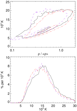
Figure 2: Convergence with resolution of the $N$-body code and the effect of cosmic variance. The top panel illustrates the $\rho-T$ distribution for the ionised gas for two $N_{p}=256^{3}$, $N_{g}=256$ realisations with the same power law model (black/solid and red/dash-dot) and a $N_{p}=512^{3}$, $N_{g}=512$ realisation (purple/dashed). The contours are at $dP/d\log\left(\rho/\langle\rho\rangle\right)/dT=3.6\times 10^{-5}\mathop{\rm K\,}\nolimits^{-1}$ and $3.6\times 10^{-4}\mathop{\rm K\,}\nolimits^{-1}$. The bottom panel shows the mass-weighted temperature distributions for the ionised gas for the same models.

The results are subject to cosmic variance and bias from the resolution of the $N$-body code and the RT grid, but not substantially. In this section we describe two extra simulations which ascertain the effects of cosmic variance and a change in the resolution parameters by comparing these with the PL08 run which they most closely match. We use the $\rho-T$ and temperature distributions (Fig. 2 top and bottom panels) to illustrate the effects. The extra simulations also show that the lack of advection in the simulations is not a source of significant error.

There are two parameters that control the spatial resolution of the simulation: the number of particles in the PM simulation, $N_{p}$, and the mesh size of the gas density grid, $N_{g}$. To estimate the variation due simply to cosmic variance, a simulation was run with a different realisation of the initial density fluctuations at the same resolution as the main body of runs ($N_{p}=256^{3}$, $N_{g}=256$). In Fig. 2, the difference between the solid (black) and dot-dashed lines (red) indicates the cosmic variance. A simulation with 8 times the mass resolution ($N_{p}=512^{3}$) and twice the RT mesh resolution ($N_{g}=512$) produced a qualitatively equivalent distribution (Fig. 2, dashed line), bracketed by the two lower resolution realisations.

The current code does not advect thermodynamic quantities. Hence if a dense halo has a high velocity, the gas in the halo is not properly modelled. The error from the lack of advection is not easy to quantify, but it is not believed to be large. The error is more prominent when cells are smaller since moving gas is more likely to cross a smaller cell. The comparison of the $256^{3}$ runs to the higher-resolution $512^{3}$ run (Fig. 2) demonstrates little variation.

4 Simulation results

The simulations provide information for two epochs of interest: the period during which the gas is being ionised and the post-ionisation epoch. Our primary focus in this paper is the post-ionisation temperature of the gas, but future telescopes such as the Low Frequency Array (LOFAR), the Mileura Widefield Array (MWA), and eventually the Square Kilometre Array (SKA), will be able to probe the epoch of ionisation itself via the red shifted 21cm line of neutral hydrogen (see Furlanetto et al., 2006, for a review). The reionisation epoch will be the topic of a future paper.

In this section, we focus on the thermal state of the gas as established by the passage of an individual ionisation front. The reionisation process involves the overlap of such fronts. The ionisation fractions of the gas after the reionisation epoch will be constantly reset as the gas sees ionising photons from an increasing number of sources, both because of the time needed for photons to reach the gas and as new sources turn on (while older ones die). These effects are not accounted for by our single I-front models. The temperature of the gas, however, is nearly insensitive to the continual resetting of the level and shape of the ionising photon background (Meiksin, 1994; Hui & Gnedin, 1997). It is instead determined by the reionisation process itself and the subsequent evolution of the physical state of the IGM. We here explore the evolution of IGM temperature as computed in our simulations. A principal goal is to determine if the temperature of the ionised IGM is dependent on the nature of the ionising source. We find that it is, and in §4.3 we quantify and discuss the magnitude of this effect and some of its consequences for the ionisation structure of the IGM.

The simulation results also permit us to explore a few other issues related to the reionisation of the IGM. Clumping of the gas will generally impede the propagation of ionisation fronts. We evaluate the importance of this effect in §4.2. Because of the inclusion of helium ionisation in our simulations, we are able to examine the ratio of He $\rm\scriptstyle II$ and He $\rm\scriptstyle III$ to H $\rm\scriptstyle I$ in the ionised IGM prior to the epoch of complete He $\rm\scriptstyle II$ reionisation. We discuss these results in §4.5.

But first, to justify the effort put into the implementation of RT in our code, we make a comparison with the optically thin approximation in §4.1.

4.1 Comparison with the optically thin approximation

Neglecting RT can underestimate temperatures by a factor of a few (Abel & Haehnelt, 1999; Bolton et al., 2004; Bolton & Haehnelt, 2007). The importance of including radiative transfer effects during reionisation to obtain accurate temperatures is best illustrated by comparing against a simulation using the optically thin approximation (OTA). Simply put, the OTA means all points not near a source receive the same average radiation field. The approximation works fairly well because any gas dense enough to self-shield is also dense enough to reach thermal balance. So the post-ionisation temperature is essentially insensitive to the details of reionisation. The approximation fails, however, to properly treat low density gas, because the time to reach thermal equilibrium in low density gas exceeds the Hubble time at high redshifts. As a consequence, the low density gas retains a memory of the reionisation details. This is particularly important when low density gas is shielded from the oncoming I-front by dense structures because of their role in hardening the spectrum of the radiation field.

Figure 3: Effects of optically thin approximation. The top panels illustrate the $\rho-T$ distribution without (left) and using (right) the optically thin approximation. The lower panels show the modification to the volume-weighted (left) and mass-weighted (right) temperature distributions produced without (solid) and with (dot-dashed) the approximation. The volume-weighted distribution is affected more because most of the volume of the Universe contains underdense regions, which retain a memory of the reionisation process.

To compare our results with those using the OTA, we performed a simulation in which the cumulative optical depth to any point was set to zero, mimicking the OTA. The $\rho-T$ and temperature distributions for the PL08 model with and without the approximation are illustrated in Fig. 3. Overall the distributions are similar. Since different regions are exposed to different spectra without the OTA, there is more spread than when the OTA is used. The hardening of the spectrum due to selective absorption of low-energy photons heats the gas, particularly in the less dense regions. A high density spur of decreasing temperature with increasing density is produced in both simulations, resulting from the establishment of thermal balance between photoionisation heating and atomic cooling (Meiksin, 1994).

4.2 Clumping

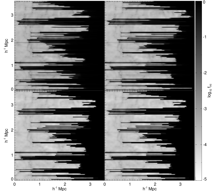
Figure 4: The H $\rm\scriptstyle I$ fraction at $z=6$. From top-left to bottom-right the panels correspond to PL20, MQ20, SB20, and HY20. (The hard source has not yet turned on in the hybrid model, so the simulation at this point is identical to the starburst run.) The ionising flux is incident from the left. Distances are in proper units.

It has long been recognized that clumping of the IGM gas may substantially slow the propagation of I-fronts due to the increased rate of radiative recombinations (Shapiro & Giroux, 1987; Meiksin & Madau, 1993; Madau & Meiksin, 1994). Estimates of the importance of clumping have varied, but recently tend toward only a moderate slowdown of the I-fronts (Sokasian et al., 2003; Meiksin, 2005; Ciardi et al., 2006) with the resistance increasing with time as clumping increases (Iliev et al., 2005). In our simulations, the slowing of the I-fronts in individual lines of sight leads to shadows in the ionisation maps, as shown in Figure 4.

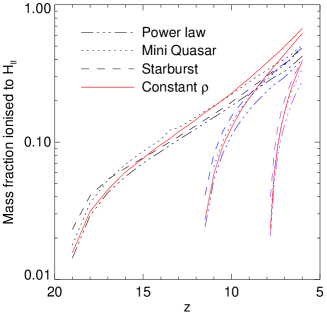
Figure 5: Fraction of the simulation volume reionised for three models, compared with the case for a uniform density IGM at the mean density. The hybrid model follows the same history as the starburst model prior to $z=6$. A simple model in which a uniform density gas ($\rho=\Omega_{g}\rho_{c}[1+z]^{3}$) is ionised by a constant flux of ionising photons is plotted as the solid line. There are three separate redshifts at which the ionising flux is turned on. All the models initially ionise the gas faster than the uniform density case as the I-front sweeps into underdense regions. Clumping eventually slows down the growth of the H $\rm\scriptstyle II$ filling factor by an amount depending on the spectral shape.

We have estimated the role clumping may play in delaying reionisation by comparing the growth of the H $\rm\scriptstyle II$ filling factor in the simulations with that predicted for a uniform IGM at the mean baryon density up to $z=6$, at which point overlapping I-fronts would complete the reionisation. Introducing structure into the IGM actually results in a moderate increase in the rate at which the filling factor of ionised gas grows in the early stages, as shown in Fig. 5. This is because most of the volume of the Universe is underdense. Once half of the volume is reionised, the filling factor converges to the uniform density prediction, with a small slowdown depending on the spectral shape of the source. The evolution of the mass-weighted fraction of ionised hydrogen follows a similar trend including the more rapid rise than the uniform density case at early times. By $z=6$, however, the fraction grows substantially less rapidly, with 50 per cent to a factor of two less mass ionised than for the uniform density prediction. The slower growth for the mass-weighted case vs the volume filling factor is expected since it takes longer for the I-front to penetrate the densest regions which contain proportionally more mass.

It is possible the amount by which the I-front slows down is underestimated because of the deficit of small dense structures like Lyman Limit Systems in $N$-body simulations (Gardner et al., 1997; Meiksin & White, 2004). A definitive result may need to await hydrodynamical simulations that reproduce the statistics of Lyman Limit Systems and denser intergalactic structures.

4.3 Temperature

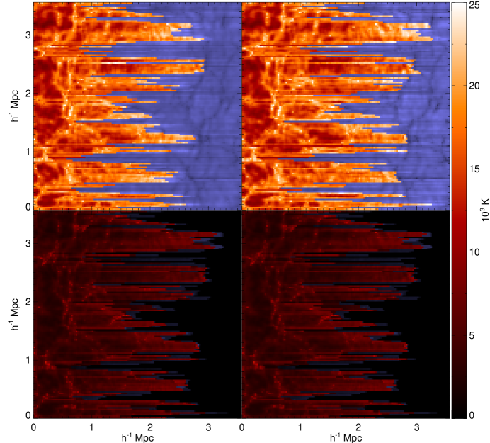
Figure 6: The temperature at $z=6$. From top-left to bottom-right the panels correspond to PL20, MQ20, SB20, and HY20. (The hard source has not yet turned on in the hybrid model, so the simulation at this point is identical to the starburst run.) The ionising flux is incident from the left. Only regions for which $f_{\rm HI}<0.1$ are shown. The remaining gas (masked as blue) would be ionised by other sources.

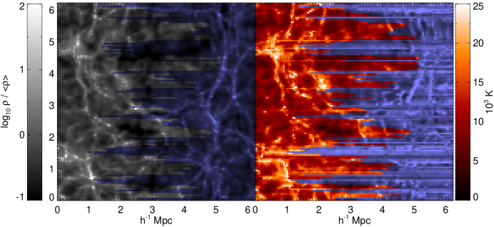
Figure 7: Density distribution (left) and temperature map at $z=3$. The temperature map is from PL20. Only regions for which the gas is ionised prior to $z=6$ are shown, the remaining regions are masked as blue.

Figure 6 is a map of the temperature distribution at a redshift of $z=6$. Figure 7 shows a similar map for the power-law model at $z=3$. In both maps, only regions in which the H $\rm\scriptstyle I$ was ionised ($f_{\rm HI}<0.1$) at $z=6$ are shown. (The remaining gas would have been ionised by a different ionisation front or fronts by this time.) We immediately see a variety of effects that will be explored quantitatively later. First, the gas temperature in the miniquasar model is virtually identical to that of the simple $\alpha=0.5$ power law. Second, the starburst model produces the coolest ionised gas. (At this stage, the hybrid and pure starburst models are identical.) Third, the highest temperatures are typically found just behind the H $\rm\scriptstyle II$ I-front. Fourth, a “streaking” effect is apparent. The gas temperature downstream of a dense clump of gas is enhanced compared with the surrounding gas as a result of delayed ionisation. The enhancement persists until $z=3$. Finally, when compared with the gas density, all the models produce gas temperature structure that traces the large-scale gas structure, as illustrated in Fig. 7. The relation, however, is not one of simple proportionality, as we will see below. For instance, because the most recently ionised gas tends to be hotter at a given density, the temperature tends to increase towards the right (because the I-front passes from left to right), as shown in Fig. 6.

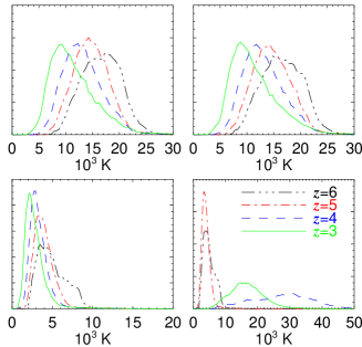
Figure 8: The volume-weighted temperature distribution at $z=6$, 5, 4 and 3 for the gas ionised before $z=6$ only. From top-left to bottom-right the panels correspond to the power-law, miniquasar, starburst, and hybrid model. The colours/line type distinguish the redshifts, with $z=6$ black/dash-dot-dot-dot, $z=5$ red/dash-dot, $z=4$ blue/dashed, and $z=3$ green/solid. Note the change in the temperature scale for the various models.

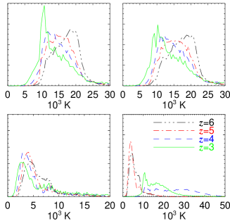
Figure 9: The mass-weighted temperature distribution at $z=6$, 5, 4 and 3 for the gas ionised before $z=6$ only. From top-left to bottom-right the panels correspond to the power-law, miniquasar, starburst, and hybrid model. The colours/line type distinguish the redshift, with $z=6$ black/dash-dot-dot-dot, $z=5$ red/dash-dot, $z=4$ blue/dashed, and $z=3$ green/solid. Note the change in the temperature scale for the various models.

The gas temperatures distinguish the various models at all redshifts. The temperature distributions of the gas ionised by $z=6$, both volume-weighted (Fig. 8) and mass-weighted (Fig. 9), show clear differences for the different model spectra. At $z=3$, for the power-law and miniquasar models, the temperatures span 8 to $28\times 10^{3}\mathop{\rm K\,}\nolimits$ (90 per cent of the gas mass with 5 per cent below the range and 5 per cent above) with a mass-weighted mean of $15\times 10^{3}\mathop{\rm K\,}\nolimits$. The hybrid model has a hotter tail in its distribution, ranging from $\sim 10$ to $31\times 10^{3}\mathop{\rm K\,}\nolimits$ with a mass-weighted mean of $17\times 10^{3}\mathop{\rm K\,}\nolimits$. Gas two to three times cooler is produced by the starburst model. For this model, the temperatures at $z=3$ range from 2000 to 17000 K with the mass-weighted mean at $9000\mathop{\rm K\,}\nolimits$. The distributions are, however, highly skewed with mass-weighted modes at $11000\mathop{\rm K\,}\nolimits$ for the power-law, miniquasar, and hybrid spectra and $3000\mathop{\rm K\,}\nolimits$ for the starburst spectrum.

There are few direct determinations of the IGM gas temperature. The measured Doppler parameters on their own provide only an upper limit since the lines may be velocity broadened (e.g. due to microturbulence). If metal lines are present, however, the thermal and kinematic contributions are separable. By simultaneously fitting C $\rm\scriptstyle IV$ and Si $\rm\scriptstyle IV$ absorbers, Rauch et al. (1996) found average temperatures of $\simeq 38000\mathop{\rm K\,}\nolimits$ for systems with $\log_{10}n_{\rm H\hskip 1.0pt\scriptscriptstyle I}>14$. Only the hybrid model is able to achieve temperatures of $T\simeq 40000\mathop{\rm K\,}\nolimits$ (Figures 8 and 9).

We have tested that the redshift at which the source turns on is not a significant factor. Save for a slight shift to higher temperatures for the $z_{\rm on}=8$ models, the curves are nearly identical. This is because the incident ionising flux has been normalised to a common value for all the cases so that by $z~{}\lower 2.15277pt\hbox{$\buildrel<\over{\sim}$}~{}8$ the reionisation proceeds in a nearly identical manner. Changing the epoch of reionisation would change the temperature in the low density gas at later times. This effect is not explored here.

Figure 10: The $\rho-T$ distribution at $z=3$ for the gas ionised by $z=6$ only. From top-left to bottom-right the panels correspond to PL20, MQ20, SB20, and HY20. The contour intervals are spaced by a factor of $\sqrt{1}0$.

As we showed above, the use of full radiative transfer instead of an optically thin approximation not only further heats the gas, but it spreads the $\rho-T$ distribution away from a tight power law (Fig. 3). The spread in temperatures is greatest for gas with $\rho/\bar{\rho}<1$. The spectrum of the ionising radiation is modified by preferential absorption of the lower frequency photons as they pass through the gas. The modification hardens any spectrum, but is most influential to spectra that already have a hard component. Hence, the spread should be largest for harder spectra. Figure 10, which maps the $\rho-T$ distribution at $z=3$ for the ionised gas for PL20, MQ20, SB20, and HY20, confirms the larger spread in the harder spectra. Also confirmed is the similarity of the state of the gas in the models with the power-law and miniquasar spectra.

Table 4: Fits to the polytropic relation, $T=T_{0}(\rho/\bar{\rho})^{\gamma-1}$ of the gas for which $f_{\rm H\hskip 1.0pt\scriptscriptstyle I}<0.1$ by $z=6$. The errors are to the fits and not indicative of the distribution in the $\rho-T$ plane.

		$z$
		6	5	4	3
	$T_{0}[\mathop{\rm K\,}\nolimits]$	$17900\pm 100$	$16900\pm 150$	$15400\pm 140$	$14600\pm 200$
PL20	$\gamma$	$1.29\pm 0.01$	$1.40\pm 0.01$	$1.52\pm 0.01$	$1.58\pm 0.01$
	$T_{0}[\mathop{\rm K\,}\nolimits]$	$17900\pm 120$	$16950\pm 170$	$15500\pm 150$	$14500\pm 160$
MQ20	$\gamma$	$1.34\pm 0.01$	$1.44\pm 0.01$	$1.52\pm 0.01$	$1.57\pm 0.01$
	$T_{0}[\mathop{\rm K\,}\nolimits]$	$4200\pm 130$	$4070\pm 50$	$3720\pm 20$	$3515\pm 11$
SB20	$\gamma$	$1.44\pm 0.03$	$1.43\pm 0.01$	$1.47\pm 0.01$	$1.553\pm 0.002$
	$T_{0}[\mathop{\rm K\,}\nolimits]$	$4200\pm 110$	$4040\pm 50$	$29250\pm 250$	$18600\pm 100$
HY20	$\gamma$	$1.42\pm 0.03$	$1.42\pm 0.01$	$-0.0363\pm 0.009$	$1.134\pm 0.005$

Pseudo-hydrodynamical models of the IGM usually adopt a polytropic equation of state for the gas. We fit a polytropic relation, $T=T_{0}(\rho/\bar{\rho})^{\gamma-1}$, to the $\rho-T$ distributions at $z=6$, 5, 4 and 3. The results are shown in Table LABEL:table.PolyFits. Note that the errors are for the coefficients and not an indication of the spread of the $\rho-T$ distribution, which is not particularly well-described as a single polytropic dependence. For comparison, for the OTA run, for which local heating is balanced by local cooling, we find $T_{0}=13780\pm 40$ and $\gamma=1.527\pm 0.003$ at $z=3$, with less spread than found when radiative transfer is incorporated. Together, these very different simulations imply a local balance between heating and cooling still dominates the setting of the polytropic index.

Generally $\gamma=1$ is assumed to be the theoretical lower limit, corresponding to isothermality. Most of the fits indeed show $\gamma>1$. The exception is the value of $\gamma$ for the hybrid model. Soon after the QSO starts ionising He $\rm\scriptstyle II$, lower values of $\gamma$ occur, including $\gamma<0$ at $z=4$. This arises because of the poor representation a polytrope gives of the wide spread in temperatures. Any applications restricting to $\gamma>1$ may therefore be excluding a description of the thermal behaviour of the IGM during the He $\rm\scriptstyle II$ reionisation epoch. At the other extreme, for all models the index is lower than the adiabatic index, $\gamma_{\rm ad}=5/3$, reflecting the influence of radiative cooling in high-density regions.

The polytropic fits resulting from the simulations may be compared with those of Schaye et al. (2000) to Keck HIRES spectra. These authors find $T_{0}\approx 2.2\pm 0.2\times 10^{4}$ K and $\gamma\approx 1.0\pm 0.1$ at $z\approx 3$, values most consistent with the late He $\rm\scriptstyle II$ reionisation hybrid model.

4.4 Ionisation rates

Figure 11: Distribution functions for the ionisation rates at $z=6$. The distributions from the various species are distinguished as indicated. Only rates from regions with ionised hydrogen ($f_{\rm HeII}<0.1$) are shown. From top to bottom, the panels correspond to the power-law, miniquasar, and starburst models. (The hybrid model is identical to the starburst model at this epoch.) The only contribution to the starburst distribution comes from hydrogen. Note the different $\Gamma$ range for the starburst model. Also note that the distributions for the individual species are normalised independently for clarity. All the distributions show extensive tails toward low values resulting from the absorption of photoionising photons by the IGM.

The varying optical depth to ionising photons results in fluctuations in the ionising background. The ionisation background is parametrized by the ionisation rate, $\Gamma$, which is the number of photoionisations per atom per unit time. A long tail towards low ionisation rates is found, as shown in Fig. 11. The sharp cut-off at the high end corresponds to low optical depth to the source leading to negligible filtering of the source spectrum. Filtering decreases the ionising photon flux, lowering $\Gamma$.

A tail in the $\Gamma$-distribution is similarly found in the simulations of Maselli & Ferrara (2005), although without the sharp cut-off at the high end. They model a uniform source distribution filtered through the IGM, accounting for the radiative transfer of the ionising photons using a Monte Carlo algorithm. The absence of the sharp upper cut-off in the simulations of Maselli & Ferrara (2005) is consistent with the discreteness effects of their Monte Carlo radiative transfer approach. In the presence of a population of randomly distributed local ionisation sources, Meiksin & White (2003) show that the sharp cut-off would be replaced by a power-law tail varying as $\Gamma_{\rm HI}^{-2.5}$.

4.5 Helium

The presence of helium alters the temperature of the IGM after reionisation by an amount that depends on the reionisation scenario. The epoch of helium reionisation (ionisation of He $\rm\scriptstyle II$ to He $\rm\scriptstyle III$) is still unknown. Measurements of the He $\rm\scriptstyle II$ Ly$\alpha$ optical depth suggests it occurred at $z~{}\lower 2.15277pt\hbox{$\buildrel<\over{\sim}$}~{}3$ (Zheng et al., 2004; Reimers et al., 2005), which is consistent with the expected epoch of He $\rm\scriptstyle II$ reionisation by QSO sources with soft spectra (Meiksin, 2005). Measurements of the Ly$\alpha$-forest Doppler parameter, $b$, permit an estimate of the IGM temperature; Theuns et al. (2002) and Ricotti et al. (2000) claim a temperature jump of about a factor of two to three at $z\ga 3$. During the reionisation process, and prior to its completion, large fluctuations in the He $\rm\scriptstyle II$ to H $\rm\scriptstyle I$ absorption signatures may be expected, as the He $\rm\scriptstyle II$-ionising metagalactic UV background will show large spatial variations.

We examine the predictions for these fluctuations from our simulations prior to the completion of He $\rm\scriptstyle II$ reionisation, by which time the He $\rm\scriptstyle III$ I-fronts have completely overlapped.

4.5.1 Thermal effects of helium

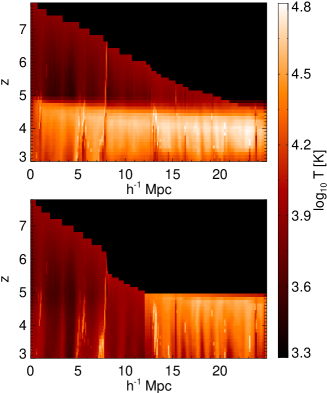
Figure 12: The importance of helium in the hybrid model. Illustrated is the evolution of the temperature of a single line of sight in a HY08 simulation with (top) and without (bottom) helium. The transition between starburst and power-law spectrum occurs between $z=5$ and 4.

The highest temperatures are produced by the hybrid model. The high temperatures are directly attributable to the presence of helium. In the hybrid model, the irradiating spectrum undergoes a transition from a starburst to a power-law spectrum between $z=5$ and 4. As a consequence, the hydrogen I-front precedes the helium I-front. Since the temperature of ionised gas cannot be raised significantly by changing the radiation field, no matter how hard the spectrum (barring extreme cases like a pure x-ray spectrum), without helium the harder power-law spectrum has no effect on the temperature of the gas previously ionised by the starburst spectrum. Gas that has not yet been ionised is heated to higher temperatures than that ionised by the starburst spectrum since more energy, $h(\nu-\nu_{0})$, is liberated per ionisation. In Fig. 12, bottom panel, the differential heating in a hybrid model without helium ($Y=0$) is illustrated. The gas ionised prior to the transition to the power-law spectrum remains unaffected by the transition. The gas previously unionised is ionised and heated to higher temperatures. With helium (top panel of Fig. 12) the transition of the spectrum heats all the gas along the line of sight. This is not surprising since the ionisation of helium introduces additional heating. What is notable is that the gas is heated to higher temperatures than for the case of a power-law spectrum ionising a completely neutral medium ($\sim 30000\mathop{\rm K\,}\nolimits$ versus $\sim 16000\mathop{\rm K\,}\nolimits$, see Fig. 8).

A He $\rm\scriptstyle III$ I-front passing through H $\rm\scriptstyle II$-dominated gas leads to a larger jump in temperature than a H $\rm\scriptstyle II$ front passing through He $\rm\scriptstyle III$-dominated gas. (Note that in both cases, the final state is fully ionised.) The temperature-entropy relation, Eq. 9, accounts for the differential temperature jumps. In the case of the He $\rm\scriptstyle II$-He $\rm\scriptstyle III$ transition in a H $\rm\scriptstyle II$-dominated gas, the mean molecular weight $\mu$ is reduced by only 7 per cent, leaving any gain in entropy to translate into a gain in temperature. In the alternate case of the H $\rm\scriptstyle I$-H $\rm\scriptstyle II$ transition in a gas where He $\rm\scriptstyle III$ is the dominate helium species, $\mu$ drops by 45 per cent, almost halving the gain in entropy. There is still a net gain in temperature, but it is only about 10 per cent.

The shallow $\rho-T$ profile in the hybrid model results from hotter low-density gas compared with the other models (Fig. 10, lower-right panel). The high temperatures following the recent He $\rm\scriptstyle II$ reionisation are retained in the low-density gas due to the long time for thermal equilibrium to be established in underdense gas (Meiksin, 1994).

4.5.2 Correction to the H $\rm\scriptstyle I$ abundances at $z<6$

Prior to overlap of the H $\rm\scriptstyle II$ I-fronts at $z\sim 6$, the ionisation state of hydrogen is properly modelled by a single source, as we have in our simulation. Equivalently, a single source is sufficient for modelling the helium fractions prior to overlap of the He $\rm\scriptstyle II$ I-fronts at $z\sim 3$. However, at $z\la 6$, a single source is insufficient to fix the hydrogen fractions, since once the Universe is reionised a given region becomes exposed to a large number of ionising sources. In particular, low-density regions once shadowed by Lyman-limit systems along the line of sight to the source driving an advancing I-front would be swept over by other I-fronts after the reionisation epoch.

In order to compare the helium ionisation fractions with the hydrogen, we need to remove the effect of the Lyman-edge shadows on the H $\rm\scriptstyle I$ from the simulation data. We do so by correcting the H $\rm\scriptstyle I$ abundances by setting $\Gamma_{\rm H\hskip 1.0pt\scriptscriptstyle I}$ to a uniform value at any given redshift and solving Eq. 1 for $n_{\rm H\hskip 1.0pt\scriptscriptstyle I}$ in the static case. Estimates of the expected distribution of $\Gamma_{\rm H\hskip 1.0pt\scriptscriptstyle I}$ after the reionisation epoch suggest it is narrowly peaked, especially for $z<4$ (Meiksin & White, 2003). We set $\Gamma_{\rm H\hskip 1.0pt\scriptscriptstyle I}$ to the mean value for the unshadowed gas at the given redshift. A negligible change to the temperatures will be generated by an increased ionisation rate after other sources are revealed, so that the local temperature produced during the reionisation phase will still apply and so sets the value of the radiative recombination coefficient $\alpha_{\rm H\hskip 1.0pt\scriptscriptstyle II}$ in Eq. 1.

The solution to $n_{\rm H\hskip 1.0pt\scriptscriptstyle I}$ is still not entirely correct, since the dense Lyman-limit systems should contain self-shielded regions within which the correction eliminates. The filling factor of the missing self-shielded regions in the corrected version, however, is much less than that of the shadowed low-density regions. We therefore applied the correction to all the H $\rm\scriptstyle I$ data at $z<6$.

4.5.3 Comparison of He $\rm\scriptstyle II$ vs H $\rm\scriptstyle I$ absorption prior to complete helium reionisation

By having two ionisation states, both at higher energies than that of H $\rm\scriptstyle I$, helium provides a means of obtaining information about the abundance of high-energy photons. The ratio of the hydrogen and helium column densities is a function of the spectral shape of the ionising radiation. Coinciding H $\rm\scriptstyle I$ and He $\rm\scriptstyle II$ absorption features in QSO spectra have been compared by Zheng et al. (2004) and Reimers et al. (2005), who find large fluctuations in the ratio of He $\rm\scriptstyle II$ to H $\rm\scriptstyle I$ column densities at $z~{}\lower 2.15277pt\hbox{$\buildrel<\over{\sim}$}~{}3$. The presence of fluctuations places constraints on helium reionisation models. Gleser et al. (2005) find the patchiness requires short QSO lifetimes ($<10\mathop{\rm Myr\,}\nolimits$) in models which attribute the patchiness to the discreteness of the QSO spatial distribution. Bolton et al. (2006) have argued for a model in which the relative number of rare He $\rm\scriptstyle II$-ionising QSOs compared with abundant He $\rm\scriptstyle I$-ionising star-forming galaxies sets the fluctuation distribution.

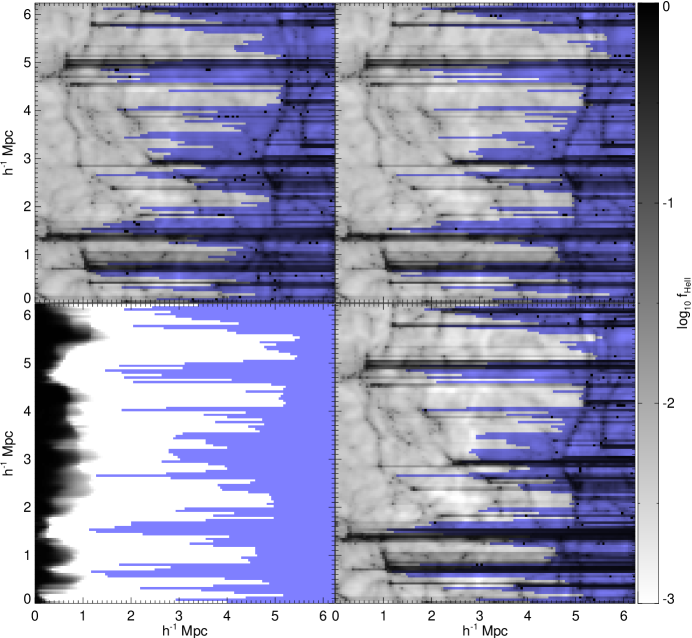
Figure 13: The He $\rm\scriptstyle II$ fraction at $z=3$. From top-left to bottom-right the panels correspond to PL20, MQ20, SB20, and HY20. The regions in which hydrogen is not ionised by $z=6$ are shaded blue.

We confine our estimates to the amount of fluctuations expected behind He $\rm\scriptstyle III$ I-fronts prior to their complete overlap, i.e., before the epoch of helium reionisation has completed. We base the analysis on the simulation results at $z=3$ (Fig. 13), which is when observations suggest He $\rm\scriptstyle II$ reionisation was nearing completion. Local sources of H $\rm\scriptstyle I$-ionising photons could introduce further fluctuations than those we find. Our simulations thus only set a lower limit to the level of fluctuations expected, arising principally from shadowing and attendant fluctuations in the He $\rm\scriptstyle II$ ionisation rate, during the final stages of He $\rm\scriptstyle II$ reionisation.

The hardness index $\eta\equiv n_{\rm He\hskip 1.0pt\scriptscriptstyle II}/n_{\rm H\hskip 1.0pt\scriptscriptstyle I}$ is a sensitive probe to the shape of the ionising background. Ionisation fraction fluctuations affect the spread in $\eta$ values while the mean value is set by the mean spectral hardness. Here we concentrate on the relative spread of the fluctuations in $\eta$, as this is independent of the shape of the spectrum. We do refer to definite values for $\eta$ from our simulations rather than arbitrarily rescaling them, but the physical effects we shall describe are not specific to any specific value $\eta$.

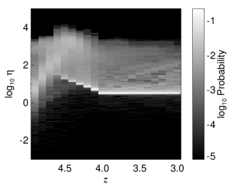
Figure 14: The evolution of the distribution of $\eta=n_{\rm He\hskip 1.0pt\scriptscriptstyle II}/n_{\rm H\hskip 1.0pt\scriptscriptstyle I}$ in the hybrid model HY20, for regions in which hydrogen was reionised by $z=6$. Although the values of $\eta$ would be shifted by a change in the spectral shape of the ionising radiation background, the relative spread is invariant. The source spectrum makes a transition from a starburst spectrum to a power law between $z=5$ and $z=4$. Because of the lack of He $\rm\scriptstyle II$-ionising photons, so that helium is not ionised to He $\rm\scriptstyle III$  the distribution of $\eta$ is much wider at $z>5$ (not shown).

The ionisation states of hydrogen and helium are expected to be linearly correlated, but dependent on the hardness of the local radiation field. This follows from radiative equilibrium, for which the rate equations for hydrogen and helium are derivable by setting $\dot{n}_{i}=0$ in Eq. 1:

$$n_{\rm H\hskip 1.0pt\scriptscriptstyle I}\Gamma_{\rm H\hskip 1.0pt\scriptscriptstyle I} = n_{e}n_{\rm H\hskip 1.0pt\scriptscriptstyle II}\alpha_{\rm H\hskip 1.0pt\scriptscriptstyle II}$$ (23)

$$n_{\rm He\hskip 1.0pt\scriptscriptstyle II}\Gamma_{\rm He\hskip 1.0pt\scriptscriptstyle II} = n_{e}n_{\rm He\hskip 1.0pt\scriptscriptstyle III}\alpha_{\rm He\hskip 1.0pt\scriptscriptstyle III}.$$

For the highly ionised gas in the simulations, $f_{\rm H\hskip 1.0pt\scriptscriptstyle I}\Gamma_{\rm H\hskip 1.0pt\scriptscriptstyle I}\simeq n_{e}\alpha_{\rm H\hskip 1.0pt\scriptscriptstyle II}$ and $f_{\rm He\hskip 1.0pt\scriptscriptstyle II}\Gamma_{\rm He\hskip 1.0pt\scriptscriptstyle II}\simeq n_{e}\alpha_{\rm He\hskip 1.0pt\scriptscriptstyle III}$, giving

$$\frac{f_{\rm He\hskip 1.0pt\scriptscriptstyle II}}{f_{\rm H\hskip 1.0pt\scriptscriptstyle I}}\simeq\frac{\alpha_{\rm He\hskip 1.0pt\scriptscriptstyle III}}{\alpha_{\rm H\hskip 1.0pt\scriptscriptstyle II}}\frac{\Gamma_{\rm H\hskip 1.0pt\scriptscriptstyle I}}{\Gamma_{\rm He\hskip 1.0pt\scriptscriptstyle II}}.$$ (24)

The ratio of $f_{\rm He\hskip 1.0pt\scriptscriptstyle II}$ to $f_{\rm H\hskip 1.0pt\scriptscriptstyle I}$ is related to $\eta$ through $\eta=(n_{\rm He}/n_{\rm H})(f_{\rm He\hskip 1.0pt\scriptscriptstyle II}/f_{\rm H\hskip 1.0pt\scriptscriptstyle I})$, where $n_{\rm He}/n_{\rm H}\approx 1/13$ ($Y=0.235$) is the number ratio of helium to hydrogen atoms. Since He $\rm\scriptstyle II$ is a hydrogen-like species, the recombination coefficients scale similarly with temperature. Over the range 10,000 K to 20,000 K, $\alpha_{\rm He\hskip 1.0pt\scriptscriptstyle III}\simeq 5.3\alpha_{\rm H\hskip 1.0pt\scriptscriptstyle II}$. Similarly, the photoionisation rates also scale but in a more complicated manner dependent on the spectrum (Eq. 2). The cross sections for H $\rm\scriptstyle I$ and He $\rm\scriptstyle II$ can be approximated by using Eq. 6 with $\beta$ and $s$ the same for hydrogen-like species, $\sigma_{\rm He\hskip 1.0pt\scriptscriptstyle II}=\sigma_{\rm H\hskip 1.0pt\scriptscriptstyle I}/4$, and $\nu_{\rm He\hskip 1.0pt\scriptscriptstyle II}=4\nu_{\rm H\hskip 1.0pt\scriptscriptstyle I}$ (Table LABEL:table.CrossSection). Taking the radiation field to have the form $J_{\nu}\propto\nu^{-\alpha}$, the integral in Eq. 2 gives for the ratio of photoionisation rates $\Gamma_{\rm H\hskip 1.0pt\scriptscriptstyle I}/\Gamma_{\rm He\hskip 1.0pt\scriptscriptstyle II}=2^{2\alpha+2}$. Combining this result with Eq. 24 and $\alpha_{\rm He\hskip 1.0pt\scriptscriptstyle III}\simeq 5.3\alpha_{\rm H\hskip 1.0pt\scriptscriptstyle II}$ gives $\eta\simeq 5.3/13\times 2^{2\alpha+2}$.

The values of $\eta$ found in the simulations fluctuate about this estimate. For PL20, for example, the volume-averaged $\hbox{$<$}\eta\hbox{$>$}_{vol}=11$ at $z=3$. However, the distribution is highly skewed; the mode and 68 percentile range is $3.3^{+3.5}_{-0.1}$. The derived relation predicts $\eta\simeq 3.2$ for $\alpha=0.5$, in good agreement with the mode. For MQ20, $\hbox{$<$}\eta\hbox{$>$}_{vol}=14$ and, like PL20, the distribution is highly skewed with the mode $3.8^{+4.0}_{-0.1}$. The $\eta$ distribution is insensitive to redshift for the power-law and miniquasar models. In the case of the hybrid model, the evolution of the $\eta$ distribution is complex after the power-law source turns on. For HY20, the evolution of the $\eta$ distribution is illustrated in Fig. 14. As the He $\rm\scriptstyle III$ I-front sweeps through the volume, $\eta$ surges to $>1000$. At the same time, the competing effect of the hardening spectrum drives the most probable $\eta$ values down. After the source spectrum has completed the transition to a power law, the most probably $\eta$ value settles at the expected value of $\eta\simeq 3.2$ while the shadowed regions provide a high-$\eta$ tail.

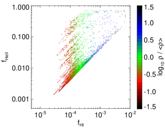
Figure 15: He $\rm\scriptstyle II$ versus H $\rm\scriptstyle I$ fractions showing dependency on density at $z=3$ for model PL20, but with a uniform H $\rm\scriptstyle I$ photoionisation rate (see text). The MQ20 and HY20 results are qualitatively similar while those for SB20 are uncorrelated owing to the paucity of helium-ionising photons. Only regions for which $f_{\rm HI}<0.1$ by $z=6$ are shown.

The fluctuations that produce the high-end tail of the $\eta$ distribution at $z=3$ arise from the attenuation of the source radiation field at the He $\rm\scriptstyle II$ ionisation threshold. Recall that we have corrected the data to remove $f_{\rm H\hskip 1.0pt\scriptscriptstyle I}$ fluctuations, hence softer (larger values of $\alpha$) local ionising fields are generated by attenuation. Variations in the local density have only a small role as they modify the local gas temperature which varies the approximation $\alpha_{\rm He\hskip 1.0pt\scriptscriptstyle III}\simeq 5.3\alpha_{\rm H\hskip 1.0pt\scriptscriptstyle II}$. Figure 15 illustrates the interplay of effects. The bulk of the gas resides along the $f_{\rm He\hskip 1.0pt\scriptscriptstyle II}/f_{\rm H\hskip 1.0pt\scriptscriptstyle I}\simeq 5.3\times 2^{2\alpha+2}$ locus in the $f_{\rm He\hskip 1.0pt\scriptscriptstyle II}-f_{\rm H\hskip 1.0pt\scriptscriptstyle I}$ plane. Attenuation leads to shadows with larger $f_{\rm He\hskip 1.0pt\scriptscriptstyle II}$ fractions, creating parallel loci of constant $f_{\rm He\hskip 1.0pt\scriptscriptstyle II}/f_{\rm H\hskip 1.0pt\scriptscriptstyle I}$. The local overdensity sets the value of $f_{\rm H\hskip 1.0pt\scriptscriptstyle I}$, as we have set $\Gamma_{\rm H\hskip 1.0pt\scriptscriptstyle I}$ to a constant value. Because of the correction to $n_{\rm H\hskip 1.0pt\scriptscriptstyle I}$, the effects of self-shielding are not seen in the $\eta$ distribution. Self-shielding would harden the spectrum, generating $\eta$ values below the bulk of the gas. This effect is seen in the uncorrected simulation data in the few regions in which it occurs.

The magnitude of $\eta$ is sensitive to the input source spectra. For instance, choosing $\alpha=2$ instead of 0.5 for the power-law spectrum would increase $\eta$ by a factor of 8 for the power-law model to values of $\eta\approx 300$. Boosting the ratio of the contribution of the galaxy to the QSO spectrum in the hybrid model would achieve a similar effect. The relative spread in the fluctuations of $\eta$, however, is independent of any overall shift in the amplitude or shape of the ionising background for regions in which both hydrogen and helium are ionised. The spread may be a useful diagnostic of the ionisation state of the IGM prior to complete He $\rm\scriptstyle II$ reionisation. Large fluctuations are found for $\eta$ (or, equivalently, in $f_{\rm HeII}/f_{\rm HI}$). At $z=3$, $\eta$ is mostly constant, but there is small fraction with a large range ($\sim 2$ dex). The extent of the range results both from the inhomogeneities in the radiation field and a wide spread in gas temperatures due to radiative transfer, particularly in the low density gas which gives rise to most of the He $\rm\scriptstyle II$ features. The spread is smaller than found by Zheng et al. (2004), who report a range of at least 2.5 dex in $\eta$ at $z\lesssim 3$. This may indicate the presence of local H $\rm\scriptstyle I$-ionising sources.

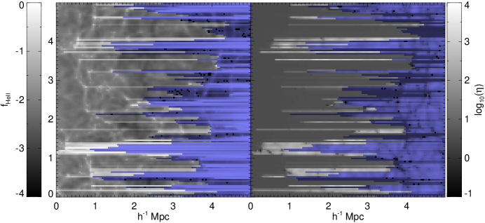
Figure 16: Comparison of the He $\rm\scriptstyle II$ ionisation fraction (left panel) and the ratio of He $\rm\scriptstyle II$ to H $\rm\scriptstyle I$ number densities $\eta=n_{\rm He\hskip 1.0pt\scriptscriptstyle II}/n_{\rm H\hskip 1.0pt\scriptscriptstyle I}$ (right panel), for the hybrid model HY20 at $z=4$. (Regions for which hydrogen is not ionised by $z=6$ are masked as blue.) A wide range in $\eta$ is found. The largest values ($\eta>1000$) correspond to regions where He $\rm\scriptstyle II$ is still incompletely reionised, with $f_{\rm He\hskip 1.0pt\scriptscriptstyle II}~{}\lower 2.15277pt\hbox{$\buildrel<\over{\sim}$}~{}1$. The H $\rm\scriptstyle I$ fractions have been corrected to a uniform photoionisation rate (see text).

Zheng et al. (2004) and Reimers et al. (2005) report some regions with $\eta>1000$, suggesting these may be regions for which He $\rm\scriptstyle II$ is still not ionised to He $\rm\scriptstyle III$. Figure 16 is a map of $\eta$ for the hybrid model HY20 at $z=4$ compared with a map of the $f_{\rm He\hskip 1.0pt\scriptscriptstyle II}$ fraction. Large $\eta$ values are found to correspond to regions of high He $\rm\scriptstyle II$ fractions. The evolution of the $\eta$ distribution for the hybrid model HY20 is illustrated in Fig. 14. At $z~{}\lower 2.15277pt\hbox{$\buildrel>\over{\sim}$}~{}4$, when the power-law source is just taking over from the starburst in magnitude, high excursions are found for $\eta$, with values reaching up to 3000. These high $\eta$ regions are associated with incomplete He $\rm\scriptstyle II$ reionisation, where $f_{\rm He\hskip 1.0pt\scriptscriptstyle II}\lesssim 1$. Lowering the redshift at which the power-law source overtakes the starburst would lower the redshift at which these high excursions occur to $z\lesssim 3$. These results suggest that Reimers et al. (2005) may have detected the He $\rm\scriptstyle II$ reionisation epoch.

In their simulations, Maselli & Ferrara (2005) find a higher value of $\eta\sim 250$, but a smaller spread of only a factor of two to three, not including the low values of $\eta$ associated with self-shielding. As discussed earlier, our single I-front simulations produce an over-abundance of shielded H $\rm\scriptstyle I$ gas at $z<6$, which we have eliminated by correcting the $n_{\rm H\hskip 1.0pt\scriptscriptstyle I}$ values to a uniform H $\rm\scriptstyle I$ photoionisation rate. Their higher value of $\eta$ results partially from the soft spectrum adopted from Haardt & Madau (1996) for QSOs with a $\alpha=1.5$ source spectrum.

Table 5: Fits to the relation $f_{\rm H\hskip 1.0pt\scriptscriptstyle I}=\alpha(\rho/\bar{\rho})^{\beta}$ for the gas for which $f_{\rm H\hskip 1.0pt\scriptscriptstyle I}<0.1$ by $z=6$. The errors are to the fits and not indicative of the distribution in the $\rho-f_{\rm H\hskip 1.0pt\scriptscriptstyle I}$ plane.

	PL20		MQ20		HY20
$z$	$\alpha$ $[\times 10^{-4}]$	$\beta$	$\alpha$ $[\times 10^{-4}]$	$\beta$	$\alpha$ $[\times 10^{-4}]$	$\beta$
6	$5.093\pm 0.003$	$0.847\pm 0.001$	$3.674\pm 0.001$	$0.8044\pm 0.006$	$2.014\pm 0.002$	$0.803\pm 0.002$
5	$3.770\pm 0.002$	$0.756\pm 0.001$	$2.784\pm 0.001$	$0.721\pm 0.001$	$1.680\pm 0.001$	$0.726\pm 0.001$
4	$2.800\pm 0.002$	$0.661\pm 0.001$	$2.083\pm 0.001$	$0.643\pm 0.001$	$1.8587\pm 0.001$	$1.066\pm 0.001$
3	$2.283\pm 0.001$	$0.6226\pm 0.0005$	$1.7239\pm 0.0004$	$0.6096\pm 0.0003$	$2.022\pm 0.002$	$0.904\pm 0.001$

Table 6: Fits to the relation $f_{\rm He\hskip 1.0pt\scriptscriptstyle II}=\alpha(\rho/\bar{\rho})^{\beta}$ for the gas for which $f_{\rm H\hskip 1.0pt\scriptscriptstyle I}<0.1$ by $z=6$. The errors are to the fits and not indicative of the distribution in the $\rho-f_{\rm H\hskip 1.0pt\scriptscriptstyle I}$ plane. Note there is negligible He $\rm\scriptstyle II$ in the HY20 run prior to $z=5$.

	PL20		MQ20		HY20
$z$	$\alpha$ $[\times 10^{-2}]$	$\beta$	$\alpha$ $[\times 10^{-2}]$	$\beta$	$\alpha$ $[\times 10^{-2}]$	$\beta$
6	$1.959\pm 0.002$	$0.775\pm 0.001$	$1.717\pm 0.002$	$0.7508\pm 0.0009$
5	$1.531\pm 0.001$	$0.695\pm 0.001$	$1.3621\pm 0.0009$	$0.6910\pm 0.0009$
4	$1.1989\pm 0.0006$	$0.6464\pm 0.0007$	$1.0514\pm 0.0004$	$0.6380\pm 0.0005$	$0.8657\pm 0.0008$	$0.978\pm 0.001$
3	$1.0107\pm 0.0005$	$0.6175\pm 0.0006$	$0.8897\pm 0.0003$	$0.6171\pm 0.0005$	$0.9295\pm 0.0008$	$0.847\pm 0.001$

We parametrize the $f_{\rm HI}$ by the gas density, $f_{\rm H\hskip 1.0pt\scriptscriptstyle I}=\alpha(\rho/\bar{\rho})^{\beta}$, and similarly for $f_{\rm HeII}$. The best fit values are provided in Tables LABEL:table.FractionFits_fH1 and LABEL:table.FractionFits_fHe2. Cosmic variance leads to errors in $\alpha$ of about 10 per cent and $\beta$ of about 2 per cent. Although the values of $\alpha$ may be readjusted by changing the magnitude of the ionisation radiation background, the values of $\beta$ are invariant for a given source spectrum. The close agreement between the values of $\beta$ for $f_{\rm H\hskip 1.0pt\scriptscriptstyle I}$ and $f_{\rm He\hskip 1.0pt\scriptscriptstyle II}$ for the respective models reflects the near linear dependence between the H $\rm\scriptstyle I$ and He $\rm\scriptstyle II$ ionisation fractions, with a weak residual dependence on density (cf Fig. 15).

The power-law dependence of ionisation fraction on density is expected if the shape of the local ionising spectrum is constant and the density and temperature are related through a power law. The equilibrium rate equation for hydrogen is $n_{\rm H\hskip 1.0pt\scriptscriptstyle I}\Gamma_{\rm H\hskip 1.0pt\scriptscriptstyle I}=n_{e}n_{\rm H\hskip 1.0pt\scriptscriptstyle II}\alpha_{\rm H\hskip 1.0pt\scriptscriptstyle II}$. Assuming almost complete ionisation, the ionisation fraction is,

$$f_{\rm H\hskip 1.0pt\scriptscriptstyle I}\simeq\frac{n_{e}\alpha_{\rm H\hskip 1.0pt\scriptscriptstyle II}}{\Gamma_{\rm H\hskip 1.0pt\scriptscriptstyle I}}.$$ (25)

We recall that the photoionisation rate, $\Gamma_{\rm H\hskip 1.0pt\scriptscriptstyle I}$, is a function of the shape of the local ionising spectrum. Assuming it is constant and that ionisation is almost complete, the neutral fraction follows $f_{\rm H\hskip 1.0pt\scriptscriptstyle I}\propto\rho\alpha_{\rm H\hskip 1.0pt\scriptscriptstyle II}$. Over the temperature range of interest, the recombination rate responds to the temperature as $\alpha_{\rm H\hskip 1.0pt\scriptscriptstyle II}\propto T^{-0.69}$. If the density and temperature are related polytropically, $T\propto\rho^{\gamma-1}$, then $f_{\rm H\hskip 1.0pt\scriptscriptstyle I}\propto\rho^{1-0.69(\gamma-1)}$. From our power-law fits in Table LABEL:table.FractionFits_fH1, the inferred values for $\gamma$ at $z=3$ are $1.547\pm 0.001$, $1.566\pm 0.001$, and $1.139\pm 0.001$ for PL20, MQ20, and HY20 respectively. For He $\rm\scriptstyle II$  the inferred values at $z=3$ are $\gamma=1.554\pm 0.001$, $1.555\pm 0.001$, and $1.222\pm 0.001$ PL20, MQ20, and HY20 respectively. The values of $\gamma$ are nearly identical to those found by directly fitting the $\rho-T$ relation in §4.3.

5 Discussion and Conclusions

We have coupled a radiative transfer code based on a probabilistic photon transmission algorithm to a Particle-Mesh $N$-body code in order to study the sensitivity of the post-ionisation temperature of the Intergalactic Medium on source spectrum. We performed multiple simulations with different spectra of ionising radiation: a power-law ($\propto\nu^{-0.5}$), miniquasar, starburst, and a time-varying hybrid spectrum that evolves from a starburst spectrum to a power law.

The power-law and miniquasar spectra produce almost identical temperature distributions, owing to their similar shapes. A greater difference of temperatures is found between the remaining models. The mass-weighted mean gas temperatures at $z=3$ are 9000 K for the starburst source, 15000 K for the power-law and miniquasar source, and 17000 K for the hybrid models. A larger difference is found between the power-law/miniquasar and hybrid model temperatures from the polytropic fits to temperature and density. A fit to the polytropic relation, $T=T_{0}(\rho/\bar{\rho})^{\gamma-1}$, gives $T_{0}=14600\pm 200$, $14500\pm 160$, $3515\pm 11$, $18600\pm 100$ and $\gamma=1.58\pm 0.01$, $1.57\pm 0.01$, $1.553\pm 0.002$, $1.134\pm 0.005$ for the power-law, miniquasar, starburst and hybrid models, respectively, at $z=3$. The errors are formal fit errors. The highest temperatures are found in the hybrid model at the end of the transition from starburst to power-law spectra ($z\approx 4$), at which time the temperatures span values up to $40,000\mathop{\rm K\,}\nolimits$, as required by measurements of C $\rm\scriptstyle IV$ and Si $\rm\scriptstyle IV$ absorption systems in the Ly$\alpha$ forest (Rauch et al., 1996).

The He $\rm\scriptstyle III$ I-front passing through H $\rm\scriptstyle II$-dominated gas leads to a larger jump in temperature than the H $\rm\scriptstyle II$ I-front passing through He $\rm\scriptstyle III$-dominated gas. Indeed, in the simulations with the power-law spectrum the temperature increase is only about 10 per cent when a trailing H $\rm\scriptstyle II$ I-front passes through gas in which helium is fully ionised. The difference is explained by the decrease in the mean molecular weight when H $\rm\scriptstyle I$ is ionised. Hence, a significant temperature change will not be produced around a hard source by the passage of a H $\rm\scriptstyle II$ I-front, in contrast to a soft source or a region in which hydrogen was fully ionised prior to helium.

The post-ionisation temperature of the IGM may be used as a key observable for identifying the nature of the sources of reionisation. While moderate to high overdensity gas establishes an equilibrium temperature in which photoionisation heating balances atomic radiative cooling processes, the equilibrium time scale exceeds a Hubble time in lower density regions, those that give rise to optically thin Ly$\alpha$ absorption systems. In contrast to optically thin reionisation models, we find a broad fanning out of the temperature-density relation for underdense regions, with temperatures exceeding $3\times 10^{4}$ K for the hybrid model with late He $\rm\scriptstyle II$ reionisation. This may help substantially in reconciling the much larger Doppler parameters measured, which have a median value of about $30\,{\rm km\,s^{-1}}$ for the optically thin Ly$\alpha$ systems at $z\approx 3$, with those predicted by simulations without radiative transfer (Meiksin et al., 2001). Even allowing for bulk motions to contribute as much as half to the line widths (in quadrature), the large measured median Doppler parameters require a gas temperature of $2.8\times 10^{4}$ K. The hybrid model comes closest to meeting this requirement. Ultimately, incorporating hydrodynamics is necessary for definitive predictions of the detailed post-ionisation state of the IGM and a precise determination of the resulting statistical properties of the Ly$\alpha$ forest.

We do not address the effect of the epoch of reionisation on the evolution of the gas temperature. Much earlier reionisation redshifts for the entire IGM will result in much cooler temperatures, primarily due to intense Compton cooling at high redshift. The effect of the reionisation epoch on the subsequent IGM temperature has been explored by Ikeuchi & Ostriker (1986), Giroux & Shapiro (1996), and Theuns et al. (2002) without radiative transfer. A degeneracy exists between the epoch of reionisation and the nature of the sources on the temperature of the IGM. If the epoch of reionisation were determined through some other means, as for instance its detection in the radio by LOFAR or the MWA, the subsequent temperature of the IGM, particularly as revealed by the widths of optically thin Ly$\alpha$ forest absorbers, could then be used to determine the nature of the sources.

Hardening of the spectrum due to passage through structures with high H $\rm\scriptstyle I$ column densities produces fluctuations in the $f_{\rm He\hskip 1.0pt\scriptscriptstyle II}/f_{\rm H\hskip 1.0pt\scriptscriptstyle I}$ ratio in the shadowed regions behind He $\rm\scriptstyle III$ I-fronts prior to complete He $\rm\scriptstyle II$ reionisation. A spread is indeed found in the data at $z~{}\lower 2.15277pt\hbox{$\buildrel<\over{\sim}$}~{}3$ (Zheng et al., 2004; Reimers et al., 2005). The observed spread of about 2.5 dex, however, exceeds that found in our simulations at $z=3$ by about a factor of three. In particular, values of $\eta>1000$ are reported by Zheng et al. (2004) and Reimers et al. (2005). It may be that local sources are required to reproduce the wider range of observed values. Alternatively, at $z~{}\lower 2.15277pt\hbox{$\buildrel>\over{\sim}$}~{}4$ values up to $\eta\approx 3000$ are found for the hybrid model, when the power-law source begins to dominate over the starburst producing partially ionised He $\rm\scriptstyle II$. Lowering the redshift at which the power-law spectrum dominates over the starburst, thus delaying the He $\rm\scriptstyle II$ reionisation epoch, would lower the redshift at which large fluctuations in $\eta$ are produced. It may be that Reimers et al. (2005) have detected the epoch of He $\rm\scriptstyle II$ reionisation.

Not explored in detail by this paper is the pre-ionisation state of the gas which is relevant to future $21\mathop{\rm cm\,}\nolimits$ detections. To correctly model the gas will require the incorporation of the production of secondary electrons and the diffuse radiation field. The production of the secondary electrons further cools the gas due both to overcoming the ionisation potential and to radiative losses from the consequent enhancement of Ly$\alpha$ collisional excitation (Shull, 1979). A copious number of Ly$\alpha$ photons could be produced in any region where helium is ionised prior to hydrogen. The photons may have important implications for the detection of the 21cm signature of the IGM, as they can decouple the spin temperature from the CMB (Madau et al., 1997). The Ly$\alpha$ photons will also be an additional source of pre-heating through recoils, although the amount is likely to be small before the scattering reaches equilibrium (Meiksin, 2006). We are currently including both hydrodynamics and the extra radiative physics in more refined models. The addition of hydrodynamics will also eliminate any limitations owing to the absence of advection.

References

- Abel & Haehnelt (1999) Abel T., Haehnelt M. G., 1999, ApJ, 520, L13, arXiv:astro-ph/9903102
- Abel et al. (1999) Abel T., Norman M. L., Madau P., 1999, ApJ, 523, 66
- Aldrovandi & Pequignot (1973) Aldrovandi S. M. V., Pequignot D., 1973, A&Ap, 25, 137
- Alvarez & Abel (2007) Alvarez M. A., Abel T., 2007, ArXiv Astrophysics e-prints, astro-ph/0703740
- Becker & et al (2001) Becker R. H., et al 2001, AJ, 122, 2850
- Black (1981) Black J. H., 1981, MNRAS, 197, 553
- Bolton et al. (2004) Bolton J., Meiksin A., White M., 2004, MNRAS, 348, L43
- Bolton & Haehnelt (2007) Bolton J. S., Haehnelt M. G., 2007, MNRAS, 374, 493, astro-ph/0607331
- Bolton et al. (2006) Bolton J. S., Haehnelt M. G., Viel M., Carswell R. F., 2006, MNRAS, 366, 1378
- Bunker et al. (2006) Bunker A., Stanway E., Ellis R., McMahon R., Eyles L., Lacy M., 2006, NewAR, 50, 94, astro-ph/0508271
- Bunker et al. (2004) Bunker A. J., Stanway E. R., Ellis R. S., McMahon R. G., 2004, MNRAS, 355, 374, astro-ph/0403223
- Cen et al. (1994) Cen R., Miralda-Escude J., Ostriker J. P., Rauch M., 1994, ApJ, 437, L9
- Choudhury & Ferrara (2006) Choudhury T. R., Ferrara A., 2006, MNRAS, 371, L55, astro-ph/0603617
- Ciardi et al. (2006) Ciardi B., Scannapieco E., Stoehr F., Ferrara A., Iliev I. T., Shapiro P. R., 2006, MNRAS, 366, 689
- Ciardi et al. (2003) Ciardi B., Stoehr F., White S. D. M., 2003, MNRAS, 343, 1101
- Cohn & Chang (2007) Cohn J. D., Chang T.-C., 2007, MNRAS, 374, 72, arXiv:astro-ph/0603438
- Fernández-Soto et al. (2003) Fernández-Soto A., Lanzetta K. M., Chen H.-W., 2003, MNRAS, 342, 1215
- Fioc & Rocca-Volmerange (1997) Fioc M., Rocca-Volmerange B., 1997, A&Ap, 326, 950
- Furlanetto et al. (2006) Furlanetto S. R., McQuinn M., Hernquist L., 2006, MNRAS, 365, 115, arXiv:astro-ph/0507524
- Furlanetto & Oh (2005) Furlanetto S. R., Oh S. P., 2005, MNRAS, 363, 1031, arXiv:astro-ph/0505065
- Furlanetto et al. (2006) Furlanetto S. R., Oh S. P., Briggs F. H., 2006, Physics Reports, 433, 181, arXiv:astro-ph/0608032
- Gardner et al. (1997) Gardner J. P., Katz N., Hernquist L., Weinberg D. H., 1997, ApJ, 484, 31
- Giroux & Shapiro (1996) Giroux M. L., Shapiro P. R., 1996, ApJS, 102, 191
- Gleser et al. (2005) Gleser L., Nusser A., Benson A. J., Ohno H., Sugiyama N., 2005, MNRAS, 361, 1399, arXiv:astro-ph/0412113
- Gnedin (2000) Gnedin N. Y., 2000, ApJ, 535, 530, astro-ph/9909383
- Gnedin & Abel (2001) Gnedin N. Y., Abel T., 2001, New Astronomy, 6, 437
- Gould & Thakur (1970) Gould R. J., Thakur R. K., 1970, Annals of Physics, 61, 351
- Haardt & Madau (1996) Haardt F., Madau P., 1996, ApJ, 461, 20
- Hui & Gnedin (1997) Hui L., Gnedin N. Y., 1997, MNRAS, 292, 27, astro-ph/9612232
- Ikeuchi & Ostriker (1986) Ikeuchi S., Ostriker J. P., 1986, ApJ, 301, 522
- Iliev et al. (2006) Iliev I. T., Ciardi B., Alvarez M. A., Maselli A., Ferrara A., Gnedin N. Y., Mellema G., Nakamoto T., Norman M. L., Razoumov A. O., Rijkhorst E.-J., Ritzerveld J., Shapiro P. R., Susa H., Umemura M., Whalen D. J., 2006, ArXiv Astrophysics e-prints, astro-ph/0603199
- Iliev et al. (2006) Iliev I. T., Mellema G., Pen U.-L., Merz H., Shapiro P. R., Alvarez M. A., 2006, MNRAS, 369, 1625
- Iliev et al. (2005) Iliev I. T., Scannapieco E., Shapiro P. R., 2005, ApJ, 624, 491
- Kuhlen & Madau (2005) Kuhlen M., Madau P., 2005, MNRAS, 363, 1069, astro-ph/0506712
- Madau & Meiksin (1994) Madau P., Meiksin A., 1994, ApJ, 433, L53
- Madau et al. (1997) Madau P., Meiksin A., Rees M. J., 1997, ApJ, 475, 429
- Madau et al. (2004) Madau P., Rees M. J., Volonteri M., Haardt F., Oh S. P., 2004, ApJ, 604, 484
- Malkan et al. (2003) Malkan M., Webb W., Konopacky Q., 2003, ApJ, 598, 878
- Maselli & Ferrara (2005) Maselli A., Ferrara A., 2005, MNRAS, 364, 1429
- Meiksin (1994) Meiksin A., 1994, ApJ, 431, 109
- Meiksin (2005) Meiksin A., 2005, MNRAS, 356, 596
- Meiksin (2006) Meiksin A., 2006, MNRAS, 370, 2025
- Meiksin et al. (2001) Meiksin A., Bryan G., Machacek M., 2001, MNRAS, 327, 296
- Meiksin & Madau (1993) Meiksin A., Madau P., 1993, ApJ, 412, 34
- Meiksin & White (2001) Meiksin A., White M., 2001, MNRAS, 324, 141
- Meiksin & White (2003) Meiksin A., White M., 2003, MNRAS, 342, 1205
- Meiksin & White (2004) Meiksin A., White M., 2004, MNRAS, 350, 1107
- Meiksin et al. (1999) Meiksin A., White M., Peacock J. A., 1999, MNRAS, 304, 851
- Miralda-Escude & Ostriker (1990) Miralda-Escude J., Ostriker J. P., 1990, ApJ, 350, 1
- Miralda-Escude & Rees (1994) Miralda-Escude J., Rees M. J., 1994, MNRAS, 266, 343
- Nakamoto et al. (2001) Nakamoto T., Umemura M., Susa H., 2001, MNRAS, 321, 593
- Osterbrock (1989) Osterbrock D. E., 1989, Astrophysics of Gaseous Nebulae and Active Galactic Nuclei. University Science Books, Sausalito, CA
- Panagia et al. (2005) Panagia N., Fall S. M., Mobasher B., Dickinson M., Ferguson H. C., Giavalisco M., Stern D., Wiklind T., 2005, ApJ, 633, L1, astro-ph/0509605
- Peebles (1968) Peebles P. J. E., 1968, ApJ, 153, 1
- Rauch et al. (1996) Rauch M., Sargent W. L. W., Womble D. S., Barlow T. A., 1996, ApJ, 467, L5+, arXiv:astro-ph/9606041
- Razoumov et al. (2002) Razoumov A. O., Norman M. L., Abel T., Scott D., 2002, ApJ, 572, 695
- Reimers et al. (2005) Reimers D., Fechner C., Hagen H.-J., Jakobsen P., Tytler D., Kirkman D., 2005, A&Ap, 442, 63
- Ricotti et al. (2000) Ricotti M., Gnedin N. Y., Shull J. M., 2000, ApJ, 534, 41, arXiv:astro-ph/9906413
- Ricotti & Ostriker (2004) Ricotti M., Ostriker J. P., 2004, MNRAS, 352, 547, arXiv:astro-ph/0311003
- Schaye et al. (2000) Schaye J., Theuns T., Rauch M., Efstathiou G., Sargent W. L. W., 2000, MNRAS, 318, 817
- Seaton (1959) Seaton M. J., 1959, MNRAS, 119, 81
- Shapiro & Giroux (1987) Shapiro P. R., Giroux M. L., 1987, ApJ, 321, L107
- Shull (1979) Shull J. M., 1979, ApJ, 234, 761
- Shull & van Steenberg (1985) Shull J. M., van Steenberg M. E., 1985, ApJ, 298, 268
- Sokasian et al. (2003) Sokasian A., Abel T., Hernquist L., Springel V., 2003, MNRAS, 344, 607
- Spergel & et al (2007) Spergel D. N., et al 2007, ApJ, in press, astro-ph/0603449
- Spergel et al. (2003) Spergel D. N., Verde L., Peiris H. V., Komatsu E., Nolta M. R., Bennett C. L., Halpern M., Hinshaw G., Jarosik N., Kogut A., Limon M., Meyer S. S., Page L., Tucker G. S., Weiland J. L., Wollack E., Wright E. L., 2003, ApJS, 148, 175
- Spitzer (1978) Spitzer L., 1978, Physical Processes in the Interstellar Medium. John Wiley, New York
- Steidel et al. (1999) Steidel C. C., Adelberger K. L., Giavalisco M., Dickinson M., Pettini M., 1999, ApJ, 519, 1, astro-ph/9811399
- Stiavelli et al. (2004) Stiavelli M., Fall S. M., Panagia N., 2004, ApJ, 610, L1, astro-ph/0405219
- Theuns et al. (2002) Theuns T., Schaye J., Zaroubi S., Kim T.-S., Tzanavaris P., Carswell B., 2002, ApJ, 567, L103
- Tittley & Couchman (2000) Tittley E. R., Couchman H. M. P., 2000, MNRAS, 315, 834, arXiv:astro-ph/9911460
- Verner & Ferland (1996) Verner D. A., Ferland G. J., 1996, ApJS, 103, 467
- Viel et al. (2002) Viel M., Matarrese S., Mo H. J., Theuns T., Haehnelt M. G., 2002, MNRAS, 336, 685, astro-ph/0203418
- Whalen & Norman (2006) Whalen D., Norman M. L., 2006, ApJS, 162, 281
- Wyithe & Loeb (2004) Wyithe J. S. B., Loeb A., 2004, Nature, 432, 194
- Yan & Windhorst (2004) Yan H., Windhorst R. A., 2004, ApJ, 600, L1, astro-ph/0312572
- Zhang et al. (1998) Zhang Y., Meiksin A., Anninos P., Norman M. L., 1998, ApJ, 495, 63
- Zheng et al. (2004) Zheng W., Kriss G. A., Deharveng J.-M., Dixon W. V., Kruk J. W., Shull J. M., Giroux M. L., Morton D. C., Williger G. M., Friedman S. D., Moos H. W., 2004, ApJ, 605, 631