The Clustering of Luminous Red Galaxies in the Sloan Digital Sky Survey Imaging Data

Abstract

We present the 3D real space clustering power spectrum of a sample of $\sim 600,000$ luminous red galaxies (LRGs) measured by the Sloan Digital Sky Survey (SDSS), using photometric redshifts. These galaxies are old, elliptical systems with strong $4000$ Å  breaks, and have accurate photometric redshifts with an average error of $\Delta z=0.03$. This sample of galaxies ranges from redshift $z=0.2$ to $0.6$ over $3,528\,{\rm deg}^{2}$ of the sky, probing a volume of $1.5h^{-3}{\rm Gpc}^{3}$, making it the largest volume ever used for galaxy clustering measurements. We measure the angular clustering power spectrum in eight redshift slices and use well-calibrated redshift distributions to combine these into a high precision 3D real space power spectrum from $k=0.005h{\rm Mpc}^{-1}$ to $k=1h{\rm Mpc}^{-1}$. We detect power on gigaparsec scales, beyond the turnover in the matter power spectrum, at a $\sim 2\sigma$ significance for $k<0.01h{\rm Mpc}^{-1}$, increasing to $5.5\sigma$ for $k<0.02h{\rm Mpc}^{-1}$. This detection of power is on scales significantly larger than those accessible to current spectroscopic redshift surveys. We also find evidence for baryonic oscillations, both in the power spectrum, as well as in fits to the baryon density, at a $2.5\sigma$ confidence level. The large volume and resulting small statistical errors on the power spectrum allow us to constrain both the amplitude and scale dependence of the galaxy bias in cosmological fits. The statistical power of these data to constrain cosmology is $\sim 1.7$ times better than previous clustering analyses. Varying the matter density and baryon fraction, we find $\Omega_{M}=0.30\pm 0.03$, and $\Omega_{b}/\Omega_{M}=0.18\pm 0.04$, for a fixed Hubble constant of $70\,{\rm km/s/Mpc}$ and a scale-invariant spectrum of initial perturbations. The detection of baryonic oscillations also allows us to measure the comoving distance to $z=0.5$; we find a best fit distance of $1.73\pm 0.12{\rm Gpc}$, corresponding to a $6.5\%$ error on the distance. These results demonstrate the ability to make precise clustering measurements with photometric surveys.

1 Introduction

The three dimensional distribution of galaxies has long been recognized as a powerful cosmological probe (Peebles, 1973; Hauser & Peebles, 1973; Groth & Peebles, 1977; Tegmark, 1997b; Tegmark et al., 1998; Goldberg & Strauss, 1998; Hu et al., 1998; Wang et al., 1999; Hu et al., 1999; Eisenstein et al., 1999). On large scales, we expect galaxy density to have a simple relationship to the underlying matter density; therefore, the clustering of galaxies is related to the clustering of the underlying matter. The two point correlation function of matter (or its Fourier transform, the power spectrum) is a sensitive probe of both the initial conditions of the Universe and its subsequent evolution. Indeed, if the matter density is well described by a Gaussian random field, then the power spectrum encodes all the information present in the field. It is therefore not surprising that a large fraction of the effort in observational cosmology has been devoted to measuring the spatial distribution of galaxies, culminating in recent results from the Two-Degree Field Galaxy Redshift Survey (2dFGRS, Cole et al., 2005) and the Sloan Digital Sky Survey (SDSS, Tegmark et al., 2004).

The spatial distribution of galaxies is also a standard ruler for cosmography. The expansion rate of the Universe as a function of redshift is a sensitive probe of its energy content, and in particular, can be used to constrain the properties of the “dark energy” responsible for the recent acceleration in the expansion (see eg. Hu, 2005; Eisenstein, 2005). One approach to measure the expansion rate is to observe the apparent size of a standard ruler (and therefore, the angular diameter distance) at different redshifts to constrain the scale factor as a function of time. The power spectrum of the galaxy distribution has two features useful as standard rulers. At $k\sim 0.01h\rm{Mpc}^{-1}$, the power spectrum turns over from a $k^{1}$ slope (for a scale invariant spectrum of initial fluctuations), to a $k^{-3}$ spectrum, caused by modes that entered the horizon during radiation domination and were therefore suppressed. The precise position of this turnover is determined by the size of the horizon at matter-radiation equality, and corresponds to a physical scale determined by the matter $(\Omega_{M}h^{2})$ and radiation densities $(\Omega_{R}h^{2})$. The other distinguishing feature is oscillations in the power spectrum caused by acoustic waves in the baryon-photon plasma before hydrogen recombination at $z\sim 1000$ (Peebles & Yu, 1970; Sunyaev & Zeldovich, 1980; Bond & Efstathiou, 1984; Holtzman, 1989; Eisenstein & Hu, 1998; Meiksin et al., 1999). The physics of these oscillations are analogous to those of the cosmic microwave background, although their amplitude is suppressed because only $\sim 1/6$ of the matter in the Universe is composed of baryons. The scale of this feature, again determined by the matter and radiation densities, is set by the sound horizon at hydrogen recombination. This feature was first observed in early 2005 both in the SDSS Luminous Red Galaxy sample (Eisenstein et al., 2005b; Hütsi, 2006) and the 2dFGRS data (Cole et al., 2005). Measuring the apparent size of both of these features at different redshifts opens up the possibility of directly measuring the angular diameter distance as a function of redshift (Eisenstein et al., 1998; Seo & Eisenstein, 2003; Linder, 2003; Matsubara & Szalay, 2003; Blake & Glazebrook, 2003; Hu & Haiman, 2003; Matsubara, 2004; Seo & Eisenstein, 2005; White, 2005; Blake & Bridle, 2005; Blake et al., 2006; Dolney et al., 2006).

Traditionally, measurements of galaxy clustering rely on spectroscopic redshifts to estimate distances to galaxies. Even with modern CCDs and high throughput multi-fiber spectrographs, acquiring them is an expensive, time-consuming process compared with just imaging the sky. For instance, the SDSS spends about one-fifth of the time imaging the sky, and the rest on spectroscopy. Furthermore, the ultimate accuracy of distance estimates from spectroscopy is limited by peculiar velocities of $\sim 1000{\rm km/s}$, a significant mismatch with the intrinsic spectroscopic accuracy of $\sim 10{\rm km/s}$.

Large multi-band imaging surveys allow for the possibility of replacing spectroscopic with photometric redshifts. The advantage is relative efficiency of imaging over spectroscopy. Given a constant amount of telescope time, one can image both wider areas and deeper volumes than would be possible with spectroscopy, allowing one to probe both larger scales and larger volumes. Furthermore, the accuracy of photometric distance estimates (Padmanabhan et al., 2005a), $c\Delta z\sim 10,000{\rm km/s}$ is more closely matched (although still not optimal) to the intrinisic uncertainties in the distance-redshift relations.

One aim of this paper is to demonstrate the practicality of such an approach by applying it to real data. We start with the five band imaging of the SDSS, and photometrically select a sample of luminous red galaxies; these galaxies have a strong 4000 Å  break in their spectral energy distributions, making uniform selection and accurate photometric redshifts possible. We then measure the angular clustering power spectrum as a function of redshift, and “stack” these individual 2D power spectra to obtain an estimate of the 3D clustering power spectrum. Using the photometric survey allows us to probe both larger scales and higher redshifts than is possible with the SDSS spectroscopic samples.

We pay special attention to the systematics unique to photometric surveys, and develop techniques to test for these. Stellar contamination, variations in star-galaxy separation with seeing, uncertainties in Galactic extinction, and variations in the photometric calibration all can masquerade as large scale structure, making it essential to understand the extent of their contamination. Furthermore, stacking the angular power spectra to measure the 3D clustering of galaxies requires testing our understanding of the photometric redshifts and their errors.

The paper is organized as follows : Sec. 2 describes the construction of the sample; Sec. 3 then discusses the measurement of the angular power spectrum and the associated checks for systematics. These angular power spectra are then stacked to estimate the 3D power spectrum (Sec. 4), and preliminary cosmological parameters are estimated in Sec. 5. We conclude in Sec. 6. Wherever not explicitly mentioned, we assume a flat $\Lambda$CDM cosmology with $\Omega_{M}=0.3$, $\Omega_{b}=0.05$, $h=0.7$, a scale invariant primordial power spectrum, and $\sigma_{8}=0.9$.

2 The Sample

2.1 The Data

The Sloan Digital Sky Survey (York et al., 2000) is an ongoing effort to image approximately $\pi$ steradians of the sky, and obtain spectra of approximately one million of the detected objects (Strauss et al., 2002; Eisenstein et al., 2001). The imaging is carried out by drift-scanning the sky in photometric conditions (Hogg et al., 2001), using a 2.5m telescope (Gunn et al., 2006) in five bands ($ugriz$) (Fukugita et al., 1996; Smith et al., 2002) using a specially designed wide-field camera (Gunn et al., 1998). Using these data, objects are targeted for spectroscopy (Richards et al., 2002; Blanton et al., 2003) and are observed with a 640-fiber spectrograph on the same telescope. All of these data are processed by completely automated pipelines that detect and measure photometric properties of objects, and astrometrically calibrate the data (Lupton et al., 2001; Pier et al., 2003; Ivezić et al., 2004). The first phase of the SDSS is complete and has produced five major data releases (Stoughton et al., 2002; Abazajian et al., 2003, 2004, 2005; Adelman-McCarthy et al., 2006). This paper uses all data observed through Fall 2003 (corresponding approximately to SDSS Data Release 3), reduced as described by Finkbeiner et al. (2004).

2.2 Photometric Calibration

Measurements of large scale structure with a photometric survey require uniform photometric calibrations over the entire survey region. Traditional methods of calibrating imaging data involve comparisons with secondary “standard” stars. The precision of such methods is limited by transformations between different photometric systems, and there is no control over the relative photometry over the entire survey region. The approach we adopt with these data is to use repeat observations of stars to constrain the photometric calibration of SDSS “runs”, analogous to CMB map-making techniques (see eg. Tegmark, 1997a). Since all observations are made with the same telescope, there are none of the uncertainties associated with using auxiliary data. Also, using overlaps allows one to control the relative calibration over connected regions of survey. The only uncertainty is the overall zeropoint of the survey, which we match to published SDSS calibrations. The above method has been briefly described by Finkbeiner et al. (2004) and Blanton et al. (2005), and will be explained in detail in a future publication.

2.3 Defining Luminous Red Galaxies

Tracers of the large scale structure of the Universe must satisfy a number of criteria. They must probe a large cosmological volume to overcome sample variance, and have a high number density so shot noise is sub-dominant on the scales of interest. Furthermore, it must be possible to uniformly select these galaxies over the entire volume of interest. Finally, if spectroscopic redshifts are unavailable, they should have well characterized photometric redshifts (and errors), and redshift distributions.

The usefulness of LRGs as a cosmological probe has long been appreciated (Gladders & Yee, 2000; Eisenstein et al., 2001). These are typically the most luminous galaxies in the Universe, and therefore probe cosmologically interesting volumes. In addition, these galaxies are generically old stellar systems with uniform spectral energy distributions (SEDs) characterized principally by a strong discontinuity at 4000 Å(Fig. 1). This combination of a uniform SED and a strong 4000 Å break make LRGs an ideal candidate for photometric redshift algorithms, with redshift accuracies of $\sigma_{z}\sim 0.03$ (Padmanabhan et al., 2005a). LRGs have been used for a number of studies (Hirata et al., 2004; Eisenstein et al., 2005a; Zehavi et al., 2005; Padmanabhan et al., 2005b), most notably for the detection of the baryonic acoustic peak in the galaxy autocorrelation function (Eisenstein et al., 2005b)

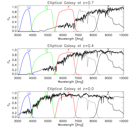
Figure 1: A model spectrum of an elliptical galaxy, taken from Bruzual & Charlot (2003), shown at three redshifts. The model assumes a single burst of star formation 11 Gyr ago and solar metallicity; the effect of evolution is not shown for simplicity. Also overplotted are the response functions (including atmospheric absorption) for the five SDSS filters. The break in the spectrum at 4000 Å, and its migration through the SDSS filters is clearly seen.

The photometric selection criteria we adopt were discussed in detail by Padmanabhan et al. (2005a) and are summarized below. We start with a model spectrum of an early type galaxy from the stellar population synthesis models of Bruzual & Charlot (2003) (Fig. 1). This particular spectrum is derived from a single burst of star formation 11 Gyr ago (implying a redshift of formation, $z_{form}\sim 2.6$), evolved to the present, and is typical of LRG spectra. In particular, the 4000 Å break is very prominent. To motivate our selection criteria, we passively evolve this spectrum in redshift (taking the evolution of the strength of the 4000 Å break into account), and project it through the SDSS filters; the resulting colour track in $g-r-i$ space as a function of redshift is shown in Fig. 2. The bend in the track around $z\sim 0.4$, as the 4000 Å break redshifts from the $g$ to $r$ band, naturally suggests two selection criteria – a low redshift sample (Cut I), nominally from $z\sim 0.2-0.4$, and a high redshift sample (Cut II), from $z\sim 0.4-0.6$. We define the two colours (Eisenstein et al., 2001, and private commun.)

$$c_{\perp}\equiv(r-i)-(g-r)/4-0.18\,\,\,,$$ (1)

$$d_{\perp}\equiv(r-i)-(g-r)/8\approx r-i\,\,\,.$$ (2)

We now make the following colour selections,

$${\rm Cut\,\,I:} \mid c_{\perp}\mid<0.2\,\,\,;$$ (3)

$${\rm Cut\,\,II:} d_{\perp}>0.55\,\,\,,$$ (4)

$$g-r>1.4\,\,\,,$$ (5)

as shown in Fig. 2. The final cut, $g-r>1.4$, isolates our sample from the stellar locus. In addition to these selection criteria, we eliminate all galaxies with $g-r>3$ and $r-i>1.5$; these constraints eliminate no real galaxies, but are effective at removing stars with unusual colours.

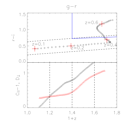
Figure 2: The top panel shows simulated $g-r$ and $r-i$ colours of an early-type galaxy as a function of redshift. The spectrum used to generate the track is the same as in Fig. 1, but evolved in redshift. Also shown are the colour cuts for Cut I (dashed, black) and Cut II galaxies (solid, blue). The lower panel shows the colours $c_{||}$ (diamonds, black) and $d_{\perp}$ (triangles, red), as a function of redshift. Also shown are fiducial redshift boundaries for Cut I (0.2 – 0.4) and Cut II (0.4 – 0.6). Note that the range in $g-r$ is identical to the range in $1+z$.

Unfortunately, as emphasized in Eisenstein et al. (2001), these simple colour cuts are not sufficient to select LRGs due to an accidental degeneracy in the SDSS filters that causes all galaxies, irrespective of type, to lie very close to the low redshift early type locus. We therefore follow the discussion there and impose a cut in absolute magnitude. We implement this by defining a colour as a proxy for redshift and then translating the absolute magnitude cut into a colour-apparent magnitude cut. We see from Fig. 2 that $d_{\perp}$ correlates strongly with redshift and is appropriate to use for Cut II. For Cut I, we define,

$$c_{||}=0.7(g-r)+1.2(r-i-0.18)\,\,\,,$$ (6)

which is approximately parallel to the low redshift locus. Given these, we further impose

$${\rm Cut\,\,I:} r_{Petro}<13.6+c_{||}/0.3\,\,\,,$$ (7)

$$r_{Petro}<19.7\,\,\,;$$

$${\rm Cut\,\,II:} i<18.3+2d_{\perp}\,\,\,,$$ (8)

$$i<20\,\,\,.$$

Note we use the $r$ band Petrosian magnitude ($r_{Petro}$) for consistency with the SDSS LRG target selection. We note that Cut I is identical (except for the magnitude cuts in Eqs. 7) to the SDSS LRG Cut I, while Cut II was chosen to yield a population consistent with Cut I (see below). This was intentionally done to maximize the overlap between any sample selected using these cuts, and the SDSS LRG spectroscopic sample. The switch to the $i$ band for Cut II also requires explanation. As is clear from Fig.1, the 4000 Å break is redshifting through the $r$ band throughout the fiducial redshift range of Cut II. This implies that the K-corrections to the $r$ band are very sensitive to redshift; the $i$ band K-corrections are much less sensitive to redshift allowing for a more robust selection.

Finally, we augment the star-galaxy separation from SDSS with the following cuts designed to minimize stellar contamination,

$${\rm Cut\,\,I:} r_{PSF}-r>0.3\,\,,$$

$${\rm Cut\,\,II:} i_{PSF}-i>0.2(21-i)\,\,,$$ (9)

$$r_{deV}>0.2\,\,,$$

where $(r,i)_{PSF}$ are the SDSS PSF magnitudes, while $r_{deV}$ is the deVaucouleurs radius of the galaxy in arcseconds.

2.4 Angular and Redshift Distributions

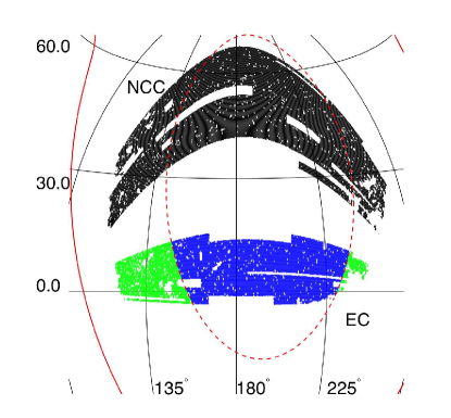
Figure 3: The angular selection function of the LRGs with the “Northern Celestial Cap” (black) and the “Equatorial Cap” (blue) shown. The lightly shaded (green) region of the Equatorial cap ($b<45^{\circ}$, shown as a dashed line) is excluded because of possible stellar contamination. The gaps in the selection function are due to missing data and exclusion around bright stars. Also shown is the Galactic equator (solid line).

Applying the above selection criteria to the $\sim$ 5500 degrees of photometric SDSS imaging considered in this paper yields a catalog of approximately 900,000 galaxies. We pixelize these galaxies as a number overdensity, $\delta_{g}=\delta n/\bar{n}$, onto a HEALPix pixelization (Górski et al., 1999) of the sphere, with 3,145,728 pixels (HEALPix resolution 9). We exclude regions where the extinction in the $r$-band (Schlegel et al., 1998) exceeds 0.2 magnitudes, as well as masking regions around stars in the Tycho astrometric catalog (Høg et al., 2000). We also exclude data from the three southern SDSS stripes due to difficulties in photometrically calibrating them relative to the rest of the data, due to the lack of any overlap. The resulting angular selection function is shown in Fig. 3. The angular coverage naturally divides into two regions, which we refer to as the “Northern Celestial Cap” (NCC) and the “Equatorial Cap” (EC), based on their positions on the celestial sphere. As discussed below, we additionally excise regions in the EC with $b<45^{\circ}$ due to possible stellar contamination. The final angular selection function covers a solid angle of 2,384 square degrees (181,766 resolution 9 HEALPix pixels) in the NCC, and 1,144 square degrees (87,263 resolution 9 HEALPix pixels) in the EC.

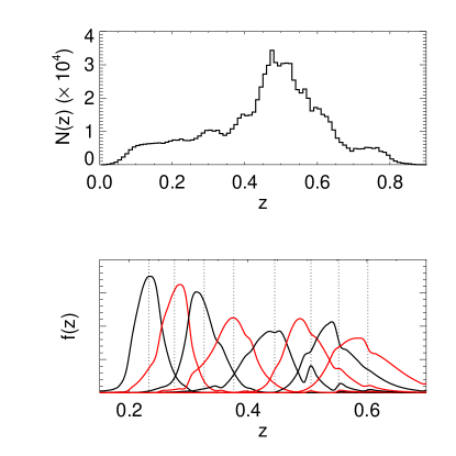
Figure 4: (Top) The photometric redshift distribution of the LRG sample. (Bottom) The deconvolved selection functions for photometric redshift slices with $\Delta z=0.05$ from $z=0.2$ to $z=0.6$. The dotted lines are the mean redshifts of each of the slices.

The calibration and accuracy of photometric redshift algorithms for this sample have been discussed in detail by Padmanabhan et al. (2005a). We compute photometric redshifts for all the galaxies in the sample using the simple template fitting algorithm described there; these redshifts have calibrated errors of $\sigma_{z}\sim 0.025$ at $z\sim 0.2$ that increase to $\sigma_{z}\sim 0.05$ at $z\sim 0.6$. The resulting photometric redshift distribution is in Fig. 4. The sample is divided into 8 photometric redshift slices of thickness $\Delta z=0.05$ ($z00$ through $z07$), and the underlying redshift distributions for each slice are estimated using the deconvolution algorithm presented in the above reference. These redshift distributions are plotted in Fig. 4, while properties of the different slices are summarized in Table 2.4.

Label	$z_{mid}$	$z_{mean}$	$N_{gal}$	$N_{gal}$	$b_{g}$
			(NCC)	(EC)
z00	0.225	0.233	16983	7942	1.74$\pm$ 0.05
z01	0.275	0.276	20377	9283	1.52$\pm$ 0.06
z02	0.325	0.326	21759	10768	1.67$\pm$ 0.07
z03	0.375	0.376	28345	12706	1.94$\pm$ 0.06
z04	0.425	0.445	41527	18767	1.75$\pm$ 0.06
z05	0.475	0.506	71131	33000	1.73$\pm$ 0.04
z06	0.525	0.552	65324	30281	1.80$\pm$ 0.04
z07	0.575	0.602	46185	20504	1.85$\pm$ 0.05

Table 1: Descriptions of the 8 $\Delta z=0.05$ redshift slices; $z_{mid}$ is the midpoint of the redshift interval, while $z_{mean}$ is the mean redshift of the slice. Also listed are the number of galaxies ($N_{gal}$) for the “Northern Celestial Cap” (NCC), and the “Equatorial Cap” (EC), and the linear bias of each redshift slice, $b_{g}$.

2.5 Sample Systematics

There are a number of systematic effects in photometric samples that contaminate clustering - stellar contamination, angular and radial modulation of the selection due to seeing variations, extinction, and errors in our modelling of the galaxy population. Fig. 5 plots the areal LRG density as a function of Galactic latitude; one would expect any leakage in the star-galaxy separation to increase at lower latitudes where the stellar density is higher. We see no increase for the NCC, but observe an increase for $b<45^{\circ}$ for the EC. This is further borne out by Fig. 6, where we plot the LRG density versus the density of stars with SDSS PSF magnitudes $18.0<r_{PSF}<19.5$, where the magnitude limits were chosen so that the SDSS star-galaxy separation is essentially perfect. Although the precise signature of such contamination on the clustering signal is unclear, we choose to be conservative and exclude regions below $b=45^{\circ}$ (Figs. 5 and  6); this reduces the area of the EC by 25%.

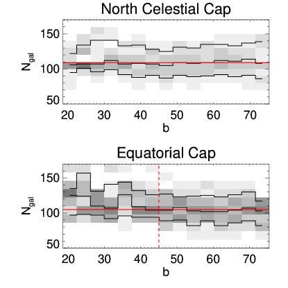
Figure 5: The average number of LRGs per resolution 6 HEALPix pixel (approximately $1\,{\rm deg}^{2}$ in area) as a function of Galactic latitude, for the two disjoint caps. The contours are 16%, 50% and 84%. There is some evidence for stellar contamination (see text for more details) at low Galactic latitudes in the Equatorial Cap; excising the region $b<45^{\circ}$ removes the problematic regions.

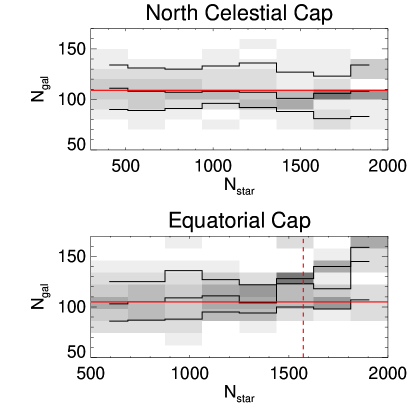
Figure 6: The same as Fig. 5 except now as a function of stellar density. The stellar density is estimated analogous to the galaxy density, selecting stars with PSF fluxes $r_{PSF}$ between 18.0 and 19.5. The vertical line shows the position of the $b<45^{\circ}$ cut in the Equatorial Cap.

To understand the nature of this contamination, we consider the subset of galaxies for which SDSS has measured spectra. We find that 118,053 (13.1%) galaxies in the photometric sample have measured spectra. Of these, 662 (0.56%) are unambiguously classified as stars (475 objects) or quasars (187 objects). The quasars are at low ($0.1<z<0.25$) redshifts, while the stars are almost entirely K and M stars, and are preferentially at lower Galactic latitudes, consistent with the above. Inspecting the imaging data shows that these are either late-type stars blended with other stars (approximately $2/3$), late-type stars blended with background galaxies (approximately $1/3$), and a smattering of star-artefact blends. Note that this explains the dependence with Galactic latitude and stellar density; one would naively expect the number of star-star blends to scale as the square of the stellar density, while the star-galaxy and star-artefact blends should roughly scale as the stellar density. We emphasize that the levels of contamination obtained this way are approximate, since the spectroscopic survey has a brighter apparent luminosity limit than our photometric catalog, and the contamination could increase with decreasing luminosity.

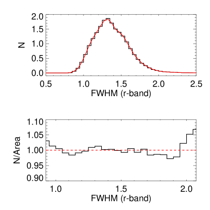
Figure 7: (top) The histogram is the (normalized) distribution of galaxies as a function of the PSF FWHM (measured in arcseconds) in the $r$ band. The (red) curve is the fraction of the total survey area with the same PSF FWHM. The agreement between them suggests that the galaxy selection algorithm is unaffected by seeing. (bottom) The galaxy surface density as a function of seeing. The two distributions are identical at the $2\%$ level except at the edges where the relevant survey area is negligible.

To test for the possible modulation of the LRG selection due to angular variations in seeing and extinction, we consider the areal density of LRGs observed as a function of seeing (as measured by the FWHM of the $r$-band PSF) and extinction (Schlegel et al., 1998). These distributions are plotted in Figs. 7 and  8. We find that the density is constant to $\sim 2\%$ over most of the range of seeing and extinction in the survey. We do observe deviations at the very edges of the distributions, but the total area with these extremes in seeing and extinction is negligible (as seen in the top panels of the figures), and therefore, do not affect clustering measurements.

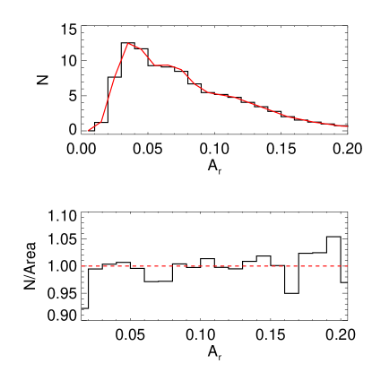
Figure 8: Analogous to Fig. 7 except with extinction in the $r$-band from Schlegel et al. (1998). We truncate at $A_{r}=0.2$ corresponding to the cut in the angular selection function.

Finally, to test sample uniformity as a function of redshift, we consider the luminosity distribution as a function of redshift. A constant luminosity distribution over the redshift range would suggest that we were selecting comparable populations of galaxies. A complication is that we must use photometric redshifts to compute absolute magnitudes; biases in the photometric redshifts could alter the inferred luminosity distributions. We estimate the magnitude of such biases from Table 2.4. At low redshifts, the photometric redshifts are essentially unbiased, whereas at high redshifts, the photometric redshifts underestimate the true redshift by about $\Delta z=0.025$, which translates into an overestimation of the magnitude by about $\Delta M=0.1-0.15$ magnitudes.

The observed conditional luminosity distribution as a function of redshift is in Fig. 9. The median luminosity is constant to approximately $\Delta M=0.1$ over the redshift range of interest, with a width of $\sim 0.7$ magnitudes (compared with a potential bias of $0.15$ magnitudes above). The distribution has two distinguishing features, a glitch at $z\sim 0.4$ and increasing luminosities at higher redshifts. The glitch at $z\sim 0.4$ corresponds to the transition between Cut I and Cut II at the point where colour tracks bend sharply in Fig. 2, and highlights a difficulty in uniformly selecting galaxies in that region. The increase in luminosities at $\sim z=0.55$ is due to the magnitude limits imposed in Cut II. Except for these two features, we conclude that our selection criteria yield an approximately uniform galaxy population from $z=0.2$ to $z=0.55$.

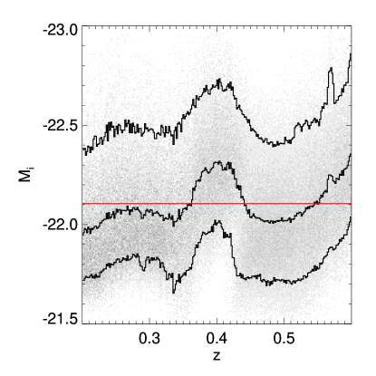
Figure 9: The conditional $i-$band magnitude distribution as a function of redshift. The absolute magnitude is computed assuming the photometric redshift. The contours show the 16%, 50%, and 84% levels, while the horizontal (red) line is the median magnitude for the entire sample. The glitch at $z\sim 0.4$ corresponds to the transition between Cut I and Cut II LRGs, while the increase at $z\sim 0.55$ is due to the magnitude limit in Cut II.

3 The Angular Power Spectrum

3.1 Projections on the sky

We relate the projected angular power spectrum to the underlying three dimensional power spectrum; our derivation follows the discussion in Huterer et al. (2001) (see also Tegmark et al., 2002, and references therein). We describe the galaxy distribution by an isotropic 3D density field, $\delta_{g,3D}$, and its power spectrum $P(k)$ defined by,

$$\langle\delta_{g,3D}({\bf k})\delta_{g,3D}^{*}({\bf k}^{\prime})\rangle=(2\pi)^{3}\delta^{3}({\bf k}-{\bf k}^{\prime})P_{g}(k)\,\,.$$ (10)

Projecting this density field on the sky along $\hat{\bf n}$, we obtain,

$$\delta_{g}(\hat{\bf n})=\frac{1}{\int\,dy\,\phi(y)}\int\,dy\,\phi(y)\delta_{g,3D}(y,y\hat{\bf n})\,\,,$$ (11)

where $y$ is the comoving distance, and $\phi(y)$ is the radial selection function. For now, we ignore the effect of peculiar velocities, and therefore do not distinguish between real and redshift space quantities. Fourier transforming the 3D density field and making use of the identity,

$$e^{-i{\bf k}\cdot\hat{\bf n}y}=\sum_{l=0}^{\infty}(2l+1)i^{l}j_{l}(ky)P_{l}(\hat{\bf k}\cdot\hat{\bf n})\,\,,$$ (12)

we obtain,

$$\delta_{g}(\hat{\bf n})=\int\,dy\,f(y)\int\frac{d^{3}k}{(2\pi)^{3}}\delta_{g,3D}(y,{\bf k})$$

$$\times\sum_{l=0}^{\infty}i^{l}(2l+1)j_{l}(ky)P_{l}(\hat{\bf n}\cdot\hat{\bf k})\,\,,$$ (13)

where $j_{l}(x)$ and $P_{l}(x)$ are the $l^{\rm th}$ order spherical Bessel functions and Legendre polynomials respectively. We define the weighting function, $f(y)$ by

$$f(y)\equiv\frac{\phi(y)}{\int\,dy\,\phi(y)}\,\,.$$ (14)

Since the density field is isotropic, we expand it in Legendre polynomials to obtain,

$$\delta_{g,l}=i^{l}\int dy\,f(y)\int\frac{d^{3}k}{(2\pi)^{3}}\delta_{g,3D}(y,{\bf k})j_{l}(ky)\,\,.$$ (15)

Figure 10: The theoretical angular power spectra for each of the redshift slices in Fig. 4. The heavy and light solid lines show nonlinear and linear auto power spectra, while the dashed lines show the cross power spectra with the adjacent slice at higher redshift. The dotted lines show the effect of redshift space distortions on both the auto and cross power spectra, assuming $\beta=0.3$. The panel $z04$ also shows the cross correlation power with $z06$ and $z07$.

In order to proceed, we assume that the selection function is narrow in redshift, allowing us to ignore the evolution of the density field. The above equation can then be written as

$$\delta_{g,l}=i^{l}\int\frac{d^{3}k}{(2\pi)^{3}}\delta_{g,3D}({\bf k})W_{l}(k)\,\,,$$ (16)

where we implicitly assume that the density field is at the median redshift of the selection function. The window function, $W_{l}(k)$, describes the mapping of $k$ to $l$ and is given by,

$$W_{l}(k)=\int dy\,f(y)j_{l}(ky)\,\,.$$ (17)

It is now straightforward to compute the angular power spectrum,

$$C_{l}\equiv\langle\delta_{g,l}\delta_{g,l}^{*}\rangle=4\pi\int\frac{dk}{k}\Delta^{2}(k)W_{l}^{2}(k)\,\,,$$ (18)

where $\Delta^{2}(k)$ is the variance per logarithmic wavenumber,

$$\Delta^{2}(k)\equiv\frac{1}{(2\pi)^{3}}4\pi k^{3}P(k)\,\,.$$ (19)

Similarly, the cross correlation between two selection functions, $\phi_{1}$ and $\phi_{2}$, is give by

$$C^{12}_{l}=4\pi\int\frac{dk}{k}\Delta^{2}(k)W_{l,1}(k)W_{l,2}(k)\,\,.$$ (20)

We have not distinguished between the galaxy and matter power spectrum above. On large scales, we simply assume

$$P_{g}(k)=b_{g}^{2}P(k)\,\,,$$ (21)

where $P_{g}(k)$ and $P(k)$ are the galaxy and matter power spectra respectively, and $b_{g}$ is the linear galaxy bias. This is a good approximation on large scales (Scherrer & Weinberg, 1998), but breaks down on smaller scales; we defer a discussion of its regime of validity, as well as the nonlinear evolution of the power spectrum to a later section.

Fig. 10 shows the predicted angular power spectra for the eight redshift distributions in Fig. 4 assuming our fiducial cosmology; also shown are the cross-correlation power spectra for adjacent slices. We assume $b_{g}=1$, and use the halofit prescription (Smith et al., 2003) to evolve the matter power spectrum into the nonlinear regime. The increase in the amplitude of the power spectrum on large scales (low $L$) with decreasing redshift is due to the linear growth of structure, while the increase in power on small scales (large $L$) is from the nonlinear collapse of structures. The “knee” in the power spectrum between $L\sim 10-30$ corresponds to the turnover in the 3D power spectrum $P(k)$, where the shape changes from $P(k)\sim k$ to $P(k)\sim k^{-3}$ (in the linear regime). This scale corresponds to the horizon at matter-radiation equality and is constant in comoving coordinates. However, with increasing radial distances to the redshift slices, the apparent angular size decreases with redshift, and we see the “knee” shift from low $L$ (large angular scales) at low redshifts to high $L$ (small angular scales) at high redshifts. This illustrates the potential use of the power spectrum as a standard ruler for cosmography; given the size of the horizon at matter-radiation equality (independent of dark energy), one can probe the evolution of the universe during the dark energy dominated phase. A second such standard ruler is the baryonic oscillations in the matter power spectrum visible at $L\sim 100$. However, its amplitude is suppressed in the individual angular power spectra by the smoothing due to the thickness of the redshift slices.

Finally, we note that the cross-correlation between adjacent slices is non-negligible. This is easily understood by considering Fig. 4, where we note that there is considerable overlap between adjacent slices. Furthermore, this overlap increases with increasing redshift due to larger photometric redshift errors; this too is reflected in the cross-correlations. Going to more widely separated slices reduces the cross-correlation due to smaller overlaps. Note that the level of correlation seen in Fig. 10 is only true on large scales; on smaller scales, uncorrelated Poisson noise (since the galaxy samples are disjoint) erases these correlations.

3.1.1 Redshift Space Distortions

The above discussion ignored the effect of peculiar velocities on the observed clustering power spectrum. For broad redshift selection functions, the projection on to the sphere erases redshift space distortions; however, as the selection function becomes narrow, they become more important. We calculate their effect below, following the formalism of Fisher et al. (1994).

We start with Eq. 11,

$$1+\delta_{g}(\hat{\bf n})=\int\,dy\,f(s)[1+\delta_{g,3D}(y,y\hat{\bf n})]\,\,,$$ (22)

where we have now written the weighting function as a function of redshift distance, $s=y+{\mathbf{v}}\cdot\hat{\bf n}$, and we have left the monopole contribution to the projected galaxy density explicit. Assuming the peculiar velocities are small compared with the thickness of the redshift slice, we Taylor expand the weight function to linear order,

$$f(s)\approx f(y)+\frac{df}{dy}({\mathbf{v}}(y\hat{\bf n})\cdot\hat{\bf n})\,\,.$$ (23)

Substituting this expression into Eq. 22, we note that at linear order, redshift space distortions only imprint fluctuations on the monopole component of the galaxy density. This allows us to separate the 2D galaxy density into two terms, $\delta_{g}=\delta_{g}^{0}+\delta_{g}^{r}$, where $\delta_{g}^{0}$ is the term discussed above, while $\delta_{g}^{r}$ are the redshift space distortions. Fourier transforming the velocity field, we find that,

$$\delta_{g}^{r}(\hat{\bf n})=\int\,dy\,\frac{df}{dy}\int\frac{d^{3}k}{(2\pi)^{3}}{\mathbf{v}}({\bf k})\cdot\hat{\bf n}e^{-i{\bf k}\cdot\hat{\bf n}y}\,\,.$$ (24)

The linearized continuity equation allows us to relate the velocity and density perturbations,

$${\mathbf{v}}({\bf k})=-i\beta\delta_{g}({\bf k})\frac{{\bf k}}{k^{2}}\,\,,$$ (25)

where $\beta$ is the redshift distortion parameter given approximately by $\beta\approx\Omega_{m}^{0.6}/b_{g}$. Substituting Eq. 25 into Eq. 24 and taking the Legendre transform, we can rewrite this equation in the form of Eq. 16 where the window function now has an additional component given by,

$$W^{r}_{l}(k)=\frac{\beta}{k}\int\,dy\,\frac{df}{dy}j_{l}^{\prime}(ky)\,\,,$$ (26)

where $j_{l}^{\prime}$ is the derivative of the spherical Bessel function with respect to its argument. By a repeated application of the recurrence relation $lj_{l-1}-(l+1)j_{l+1}=(2l+1)j_{l}^{\prime}$, and integrating by parts,

$$W^{r}_{l}(k)=\beta\int\,dy\,f(y)\left[\frac{(2l^{2}+2l-1)}{(2l+3)(2l-1)}j_{l}(ky)\right.$$

$$\left.-\frac{l(l-1)}{(2l-1)(2l+1)}j_{l-2}(ky)-\frac{(l+1)(l+2)}{(2l+1)(2l+3)}j_{l+2}(ky)\right]\,\,.$$ (27)

It is interesting to note that this result could have been equivalently derived by starting from the Kaiser (1987) enhancement of the 3D power spectrum due to redshift space distortions, $P_{g}({\bf k})\rightarrow P_{g}({\bf k})[1+\beta({\bf k}\cdot\hat{\bf n})]$, and integrating along the line of sight as in Sec. 3.1; the $l\pm 2$ spherical Bessel functions result from the coupling of the ${\bf k}\cdot\hat{\bf n}$ angular dependence to the Legendre polynomials. Also interesting is the $l\gg 0$ limit of the above equation; for $l$ sufficiently large, $\int dy\,f(y)j_{l}(y)\approx\int dy\,f(y)j_{l\pm 2}(y)$, and $W^{r}(k)$ vanishes. Physically, this corresponds to the radial velocity perturbations being erased by the projection on to the sky.

Fig. 10 shows the effects of redshift space distortions on the angular power spectra for the eight redshift slices we are considering. Note that they contribute significantly only on the largest scales ($l<\sim 30$), justifying our use of linear theory.

3.2 Power Spectrum Estimation

The theory behind optimal power spectrum estimation is now well established, and so we limit ourselves to details specific to this discussion, and refer the reader to the numerous references on the subject (Tegmark et al., 1998; Seljak, 1998; Padmanabhan et al., 2001, and references therein).

We start by parametrizing the power spectrum with twenty step functions in $l$, $\tilde{C}^{i}_{l}$,

$$C_{l}=\sum_{i}p_{i}\tilde{C}^{i}_{l}\,\,,$$ (28)

where the $p_{i}$ are the parameters that determine the power spectrum. We form quadratic combinations of the data,

$$q_{i}=\frac{1}{2}{\mathbf{x}}^{T}{\mathbf{C}}_{i}{\mathbf{C}}^{-1}{\mathbf{C}}_{i}{\mathbf{x}}\,\,,$$ (29)

where ${\mathbf{x}}$ is a vector of pixelized galaxy overdensities, ${\mathbf{C}}$ is the covariance matrix of the data, and ${\mathbf{C}}_{i}$ is the derivative of the covariance matrix with respect to $p_{i}$. The covariance matrix requires a prior power spectrum to account for cosmic variance; we estimate the prior by computing an estimate of the power spectrum with a flat prior and then iterating once. We also construct the Fisher matrix,

$$F_{ij}=\frac{1}{2}{\rm tr}\left[{\mathbf{C}}_{i}{\mathbf{C}}^{-1}{\mathbf{C}}_{j}{\mathbf{C}}^{-1}\right]\,\,.$$ (30)

The power spectrum can then be estimated, $\hat{\mathbf{p}}={\mathbf{F}}^{-1}{\mathbf{q}}$, with covariance matrix ${\mathbf{F}}^{-1}$.

A final note on implementation - the dimension of the data covariance matrix is given by the number of pixels in the data. This quickly makes any direct implementation of this algorithm impractical. We therefore use the algorithm outlined by Padmanabhan et al. (2003), modified for a spherical geometry as in Hirata et al. (2004).

3.3 Simulations

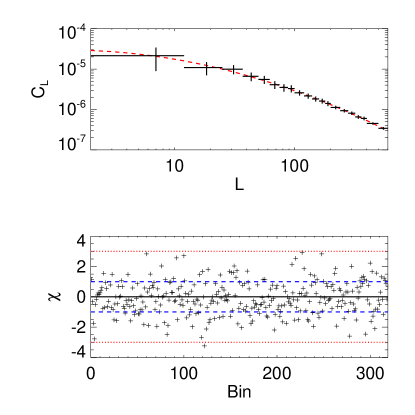
Figure 11: (top) The average recovered power spectrum from 100 simulated realizations. The dashed (red) line is the input power spectrum. The error bars are the errors per realization, and are not the error on the mean. Note that we have suppressed the input power spectrum by a constant factor relative to the expected power to avoid getting $\delta>1$; the galaxy number density was boosted by the same factor to reduce the shot noise.(bottom) $\chi$ comparing the errors on the power spectrum derived from the Fisher matrix versus those obtained from the run to run variance of the simulations for each of the eight redshift slices and the two angular caps. Assuming the density field is Gaussian, the error on the power spectrum errors ($\sigma$) is $\sigma/\sqrt{2N}$, where $N$ is the number of the simulations. Also shown are the $1\sigma$ and $3\sigma$ lines.

Before applying the above algorithm to the LRG catalog, we apply it to simulated data. In addition to testing the accuracy of our power spectrum code, we would also like to understand the correlations between the NCC and the EC, allowing us to combine separate power spectrum measurements.

In order to do so, we use the prior power spectra for each redshift slice to simulate a Gaussian random field over the entire sphere. We then Poisson distribute galaxies with probability $(1+\delta)/2$ over the survey region, trimmed with the angular selection function. One technical complication (Padmanabhan et al., 2001) is that the measured amplitude of the power spectrum results in a number of points with $|\delta|>1$, making simple Poisson sampling impossible. To avoid this, we suppress the power spectrum by a constant factor, and boost the number density of galaxies by the same factor to ensure that the shot noise is similarly suppressed. We generate 100 such simulations for the eight redshift slices and both angular caps separately, matching the observed numbers of galaxies in each case; although the different redshift bins are uncorrelated, the angular caps are based on correlated density fields. This allows us to estimate the covariance between power spectrum measurements made for the different caps. Our goal here is not to realistically simulate galaxy formation, but to test our pipelines, and the resulting measurements and errors; Gaussian simulations are sufficient for this purpose.

The results from one set of 100 simulations are shown in the top panel of Fig. 11; the recovered power spectrum agrees well with the input power spectrum. The bottom panel of the same plot compares the errors as measured by the inverse of the Fisher matrix with those obtained from the run to run variance of the simulations. Assuming Gaussianity, these errors should themselves have a relative error given by $\Delta\sigma/\sigma=1/\sqrt{2N}$ where $N=100$ is the number of the simulations. As evident from the figure, the run to run variance agrees (within the expected errors) with the errors from the Fisher matrix.

3.4 The Angular Power Spectrum

Figure 12: The measured angular power spectrum for the 8 redshift bins. The crosses show the power spectrum (and measured errors) of Cap I and Cap II combined, while the diamonds and stars are the measured power spectra of Cap 1 and Cap II separately. The solid lines are the predicted nonlinear power spectra for our fiducial cosmological model, while the dotted line shows the linear prediction. The dashed line is the nonlinear power spectrum for a model with negligible baryonic content. The vertical line marks the nominal nonlinear scale given by $k=0.1h\rm{Mpc}^{-1}$.

Fig. 12 shows the measured angular power spectrum for the eight redshift slices, with the two angular caps being measured separately. The difficulty with processing the two angular caps simultaneously is that errors in photometric calibration masquerade as large scale power. While it is possible to control these systematics in regions with overlaps in the data, the two angular caps are disconnected; therefore, any relative calibration between the two caps must be indirect (eg. considering data taken on the same night, and assuming that the calibration is constant through the night). Unfortunately, the expected power on these scales is also small ($\Delta^{2}\sim 10^{-3}$), and so we choose to be conservative and measure the angular power spectrum for the caps separately. We combine these using the simulations of the previous section to correctly take the covariances between the two caps into account. In order to avoid mixing power between different angular scales, we simply use constant weights proportional to the area (0.67 and 0.33 for the NCC and EC respectively); these are approximately the same weights that one would have obtained by inverse variance weighting. The final results are in Fig. 12.

3.5 Bias and $\beta$

Figure 13: Bias as function of redshift, as estimated for the eight redshift slices, marginalizing over redshift space distortions. Note that the fourth slice, with its anomalous bias, corresponds in redshift to the glitch seen in Fig. 9. The dashed line shows the best linear fit to the all eight bias values, while the dotted line excludes the fourth data point. Note that we have ignored the correlations between the different redshift slices for the fit.

An immediate question is whether the power spectra in Fig. 12 are consistent with being derived from a single 3D power spectrum, appropriately normalized to account for bias and the evolution of structure. We start with the linear 3D power spectrum for our fiducial cosmology, and project it to a 2D power spectrum $C_{l,gg}$, using the formalism of Sec. 3.1. We also compute the effect of redshift space distortions, whose normalization we parametrize by $\beta$, along the lines of Sec. 3.1.1, giving us two more power spectra, $C_{l,gv}$ and $C_{l,vv}$. The total power spectrum is,

$$C_{l}=b_{g}^{2}\left(C_{l,gg}+2\beta C_{l,gv}+\beta^{2}C_{l,vv}\right)\,\,,$$ (31)

where $b_{g}$ is the linear bias of the LRGs. The three power spectra represent correlations of the galaxy density with itself ($gg$), the velocity perturbations (the source of linear redshift distortions) with itself ($vv$), and their cross correlation ($gv$). We also note (as emphasized in Sec. 3.1.1) that the redshift distortions only affect the largest scales; therefore, the linear assumption is justified. We can now explore the $\chi^{2}$ likelihood surface as a function of $b$ and $\beta$ for each of the redshift slices. In practice, $\beta$ is not strongly constrained by these data, and so we marginalize over it when estimating the bias.

The best fit models are compared with the data in Fig. 12, while the bias for the eight redshift slices is in Fig. 13. We do not fit to the entire power spectrum, but limit ourselves to scales larger than the nominal nonlinear cutoff at $k=0.1h{\rm Mpc}^{-1}$; the angular scales corresponding to this restriction are marked in Fig. 12. Our starting hypothesis - that the angular power spectra are derived from a single 3D power spectrum - appears to be well motivated. Interestingly, the halofit nonlinear prescription for the matter power spectrum fits the galaxy power spectrum data down to small scales as well. The minimum $\chi^{2}$ value is 81.6 for 62 degrees of freedom, corresponding to a probability of $4.8\%$.

Fig. 13 shows that the bias increases with increasing redshift, as one would expect for an old population of galaxies that formed early in the first (and therefore most biased) overdensities. A notable exception to this trend appears to be redshift slice $z03$; however, this redshift slice corresponds to the region of the glitch in the luminosity-redshift distribution plotted in Fig. 9. If the median luminosity in this redshift slice is higher than the other slices, one would expect a higher linear bias, consistent with what is observed.

Figure 14: $\chi^{2}$ as a function of the dimensionless growth factor, $f=\beta b\sim\Omega_{m}^{0.6}$, marginalizing over bias, for all eight redshift slices combined. The dashed lines mark the $1-$ and $2-\sigma$ intervals, while the shaded region corresponds to the value of $\Omega_{m}^{0.6}$ between $z=0.2$ and $z=0.6$, assuming a present day value of $0.3$. The $\chi^{2}$ value of 81.6, for 62 degrees of freedom has a probability of $4.8\%$. Note that we have ignored the correlations between the different redshift slices.

In order to constrain $\beta$, we start from the definition that $\beta\equiv f(\Omega_{M},\Omega_{\Lambda})/b$, where $f\sim\Omega_{m}(z)^{0.6}$ is the dimensionless growth factor at redshift $z$. Assuming that the error on $f$ is larger than the variation of $\Omega_{m}$ with redshift, we approximate $f$ as a constant over the depth of the survey. We can then attempt to constrain $f$ by combining all eight redshift slices; note that for simplicity, we ignore the correlations between the slices and treat them as independant. The results are in Fig. 14. We start by noting that the width of the $\chi^{2}$ distribution is significantly larger than the variation in $f$ with redshift, justifying our starting assumption. This is a direct, albeit crude, measure of $\Omega_{m}(z\sim 0.5)\approx 0.97\pm 0.53$, consistent with our fiducial model of $\Omega_{m}(z=0.5)=0.59$.

3.6 Redshift correlations

An important test of systematics is the cross correlation between different redshift slices. For well separated slices, the cosmological correlation goes to zero on all but the largest scales; the detection of a correlation would imply the presence of systematic spatial fluctuations caused by eg. stellar contamination, photometric calibration errors, incorrect extinction corrections etc. On the other hand, the cosmological cross correlation is nonzero for adjacent slices due to overlaps in the redshift distribution, but is completely determined theoretically by the observed auto-correlation power spectra and the input redshift distributions. These cross correlations therefore test the accuracy of the estimated redshift distributions, and in particular, the wings of these distributions where they overlap.

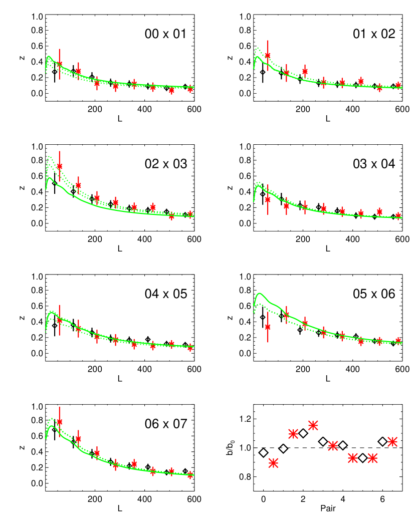
Figure 15: The Fisher z-transform of the correlation coefficient between adjacent redshift slices. The diamonds and stars are the results for the NCC and EC respectively; the errors are $2\sigma$ errors. Note that the window function is only approximately corrected; nearby bins are therefore correlated. The solid curve is the prediction for the cross correlation with the bias of both the slices fixed to the autocorrelation value, while the dotted lines show the fits allowing a variable bias. The plot in the lower right corner shows the best fit bias compared to the prediction from the autocorrelation.

For computational convenience, we estimate the cross correlations with a simple pseudo-$C_{l}$ estimator,

$$\hat{C}^{12}_{l}=\frac{1}{2l+1}\sum_{m=-l}^{l}a_{1,lm}a_{2,lm}^{*}\,\,,$$ (32)

where $a_{1,2,lm}$ are the spherical tranforms of the galaxy density. The pseudo-$C_{l}$ power spectrum is the true power spectrum convolved with the angular mask of the survey; it is therefore convenient to work with the cross correlation coefficient,

$$r^{12}_{l}\equiv\frac{\hat{C}^{12}_{l}}{\sqrt{\hat{C}^{11}_{l}\hat{C}^{22}_{l}}}=\frac{M\star C^{12}_{l}}{\sqrt{(M\star C^{11}_{l})(M\star C^{22}_{l})}}\,\,,$$ (33)

where $M\star$ represents convolutions by the angular mask. The advantage of the cross correlation is that on scales smaller than the angular mask, the effect of the angular mask approximately cancels, allowing for easy comparison with theory. It is useful to apply Fisher’s $z$-transform (Kendall & Stuart, 1977; Press et al., 1992)

$$z=\frac{1}{2}\log\left(\frac{1+r}{1-r}\right)\,\,,$$ (34)

which is well described (for $l\mbox{${}^{>}_{\sim}$}50$) by a Gaussian with mean,

$$\langle z\rangle=\frac{1}{2}\log\left(\frac{1+r_{true}}{1-r_{true}}\right)+\frac{r_{true}}{2(N-1)}\,\,,$$ (35)

and standard deviation,

$$\sigma(z)\approx\frac{1}{\sqrt{N-3}}\,\,,$$ (36)

where $N\approx(2l+1)f_{sky}$ is the number of independent modes, and $r_{true}$ is the predicted cross correlation coefficient.

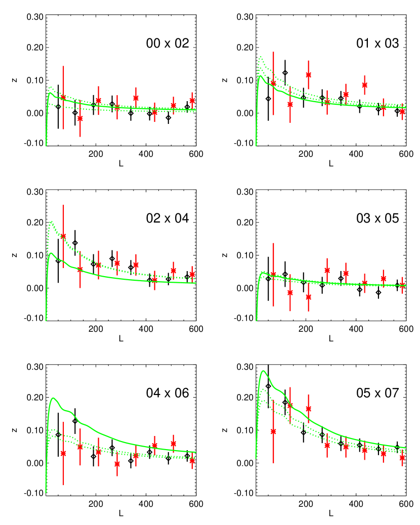
Figure 16: The same as Fig. 15 but for redshift slices separated by one redshift bin. The overlaps at low redshifts are negligible, but increase at higher redshift.

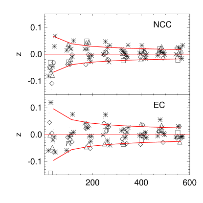
Figure 17: The Fisher z-transform of the correlation coefficient between redshift slices separated by at least two redshift slices. The curves show the $1-$ and $3-\sigma$ contours, given the null hypothesis of no correlations. Note that the window function is only approximately corrected; nearby multipoles are therefore correlated.

Figs. 15,  16,  17 show the measured cross correlations between adjacent and more widely separated slices respectively. The absence of correlations between widely separated slices indicates a lack of small scale systematics common to the different redshift slices. The cross-correlations between adjacent slices broadly agree with the predictions from the auto-correlations, although there are differences at the $\sim 10\%$ level as seen in the plot in the lower right. There are two possibilities for this disagreement. The first is that variations in the galaxy population over a redshift slice could cause the bias in the overlap region to differ from the value averaged over the entire slice. Comparing with Fig. 13, we note that slice to slice bias variations of $\sim 10\%$ are consistent with the data.

Figure 18: The change in the angular power spectrum when the $z02$ redshift distribution is shifted by $\Delta z=0.01$ [dashed], the $z03$ redshift distribution is shifted by $\Delta z=-0.01$ [dot-dashed], and $z02$ and $z03$ are shifted by $0.005$ and $-0.005$ respectively [solid]. The ratios of the angular auto power spectra are approximately 1 ($\pm 0.05$), while the ratios of the cross correlations are approximately 1.2.

A second possibility is errors in the redshift distributions. To quantify this, we model possible redshift errors by a shift in the median redshift. An example of this is shown in Fig. 18 for the $z02$ and $z03$ slices. The figure demonstrates that shifting the median by 10% of the slice width can account for the discrepancies in the cross-correlation power spectrum. Furthermore, note that the corrections to the auto-power spectra are $\sim 5\%$, and is principally a multiplicative factor that is degenerate with the bias. Finally, the above discussion also demonstrates that the cross-correlation spectra are able to constrain errors in the median redshift at the percent level.

3.7 Calibration Errors

The final systematic effect we consider is photometric calibration errors. Fluctuations in the photometric calibration will select slightly different populations of galaxies over the entire survey region, imprinting the pattern of photometric zeropoint errors on the derived density fluctuations. One expects calibration errors to result in striping perpendicular to the drift scan direction (approximately RA). These would have a characteristic scale of $\sim 0.22^{\circ}$ (the width of a camera column), corresponding to a multipole $l\sim 800$, corresponding to smaller scales than those considered in this paper. The situation is further improved by the fact that the SDSS drift-scan “strips” are often broken up into several pieces with different photometric zeropoints, further reducing the coherence length. Thus, on the angular scales used in this paper, one expects calibration errors to have an approximately white noise power spectrum.

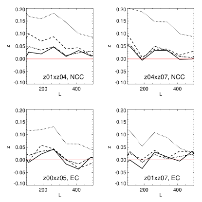
Figure 19: The effect of calibration errors on the cross-correlation power spectrum of non-adjacent redshift slices for a single simulation. The solid line shows the observed cross correlation (as the Fisher $z$-transform), while the dotted, dashed and dot-dashed lines show the effects of 5%, 2%, and 1% calibration errors.

A useful diagnostic of photometric calibration errors is the cross-correlation between redshift slices with negligible physical overlap; calibration errors will be common between both slices. Estimating the induced cross-correlation requires simulations to propagate the calibration errors through the selection criteria and photometric redshift estimation. We simulate this by perturbing the magnitude zeropoint of each camera column and filter separately; the resulting catalogs are then input into the LRG selection and photometric redshift pipelines.

Fig. 19 shows example cross-correlations for one of these simulations. The lack of an observed cross-correlation argues for photometric calibration errors $<2\%$, consistent with other astrophysical tests of the calibration (D. P. Finkbeiner, private communication). The effect of such errors on the autocorrelation measurements is subdominant to the statistical errors. Note that the survey scanning strategy makes the large scale power spectrum relatively insensitive to $\sim 1\%$ calibration errors, the expected calibration accuracy of the SDSS.

4 The 3D Power Spectrum

Although the above power spectra are a perfectly good representation of the cosmological information contained in these data, there are advantages to compressing these eight 2D power spectra into a single 3D power spectrum. The first is aesthetic; given a cosmological model, the 3D power spectrum can be directly compared to theory, in contrast to the 2D power spectra which involve convolutions by kernels determined by the redshift distributions of the galaxies (that contain no cosmological information by themselves). Furthermore, the 3D power spectrum directly shows the scales probed, and allows one to test (in a model independant manner) for features like baryonic oscillations. Finally, the 2D power spectrum requires computing the convolution kernels, making it expensive to use in cosmological parameter estimations. We however emphasize that this is (as shown below) simply a linear repackaging of the data.

4.1 Theory

Inverting a 2D power spectrum to recover the 3D power spectrum has been discussed by Seljak (1998) and Eisenstein & Zaldarriaga (2001). An important detail where the two methods differ is in how they regularize the inversion. Since the 2D spectrum is the result of a convolution of the 3D power spectrum, it is generally not possible to reconstruct the 3D power spectrum exactly given the 2D spectrum, and one must regularize the inversion. In practice, this limitation is not severe, since one would normally estimate the power spectrum in a finite number of bands; these regularize the inversion if the band width approximately corresponds to the width of the convolution kernel. This is the solution that Seljak (1998) presents. Eisenstein & Zaldarriaga (2001) consider bands that have sub-kernel width, and regularize the inversion by conditioning singular modes in an SVD decomposition. These modes are, however, given a large error, and so contain no information. We adopt the regularization scheme of Seljak (1998).

We start by writing the 3D power spectrum, $\Delta^{2}(k)$ as,

$$\Delta^{2}(k)=\delta(k)\Delta^{2}_{0}(k)\,\,,$$ (37)

where $\delta(k)$ is the sum of step functions whose amplitudes are to be determined, while $\Delta^{2}_{0}(k)$ is a fiducial power spectrum that describes the shape of the power spectrum within a bin. If we now describe both the 2D power spectrum, $C_{l}$, and and the 3D power spectrum $\delta(k)$, as vectors of bandpowers, Eq. 18 can be rewritten as a matrix equation,

$$\vec{C}_{l}={\bf W}\vec{\delta}\,\,,$$ (38)

where ${\bf W}$ is the discretized convolution kernel. The solution, by singular value decomposition or normal equations (see Press et al., 1992, 15.4), is

$${\bf C}_{\delta}^{-1}={\bf W}^{t}{\bf C}_{cl}^{-1}{\bf W}\,\,$$

$$\vec{\delta}={\bf C}_{\delta}{\bf W}^{t}{\bf C}_{cl}^{-1}\vec{C}_{l}\,\,,$$ (39)

where ${\bf C}_{cl}$ and ${\bf C}_{\delta}$ are the covariance matrices of $C_{l}$ and $\delta(k)$ respectively.

The above discussion glossed over a number of subtleties. The first is extending this formalism for $N$ 2D power spectra. If we assume that these 2D power spectra are derived from the same 3D power spectrum, one just expands $\vec{C}_{l}$ and ${\bf C}_{cl}$ to contain all the power spectra. However, in general, the 3D power spectra that corresponds to each of the 2D power spectra could differ both in their bias and nonlinear evolution. For the latter, we divide $\delta(k)$ into two sets of bands, linear bands with $k<k_{nl}$, and nonlinear bands with $k\geq k_{nl}$. We then assume that the linear bands are common to all $N$ 2D power spectra, but that there are $N$ copies of the nonlinear bands that correspond to each of the $N$ power spectra. In what follows, we assume that $k_{nl}=0.1h{\rm Mpc}^{-1}$.

Accounting for differences in bias over the different redshift slices (as seen in Fig. 13) is more involved. Naively adding $N$ bias parameters to Eq. 38 destroys the linearity of the system. One might simply use the best fit values in Fig. 13, but the fiducial model used might not correspond to the best fit model. We therefore use an iterative scheme and minimize the $L^{2}$ norm of

$$\frac{\vec{C}_{l}}{\vec{b}}-{\bf W}\vec{\delta}\,\,,$$ (40)

where $\vec{b}$ is a vector of the biases (squared); these biases are then held constant and the inversion is performed as above.

The next subtlety involves the choice of $\beta$ in order to compute the redshift space distortions. As Fig. 14 shows, these data only weakly constrain $\beta$, and therefore we choose to use the linear theory prediction for $\beta$ (more precisely for $f=b\beta$), since the redshift space distortions only affect the largest (and therefore most linear) scales.

Finally, correctly combining the different redshift slices requires knowing the covariance between the slices. However, the power spectrum estimation in Sec. 3.4 treats each slice independently and does not return the covariance between the different slices. In order to estimate the magnitude of this effect, we start by observing that the covariance between redshift slices $1$ and $2$ for multipole $l$, $C(l_{1},l_{2})$ is

$$C(l_{1},l_{2})\sim 2[C^{12}_{l}]^{2}$$ (41)

where $C^{12}_{l}$ is the angular cross power spectrum. Using the fact that the above relation is exact for full sky surveys, we substitute this into Eq. 39, and use the results with and without these redshift correlations to scale the errors we obtain from the inversion. We discuss the validity of these approximations below.

4.2 Results

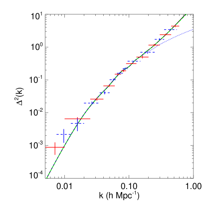
Figure 20: The 3D power spectrum obtained by inverting the 8 2D power spectra, normalized to the $z=0.2$ power spectrum on linear scales ($k<k_{nl}$), and uses the $z=0.2$ bands for the nonlinear bands. The solid and dashed lines represent binnings B1 and B2 respectively, and the two power spectra are consistent. Note that these binnings are not independent, and must not be combined for fitting. Also shown are the nonlinear power spectrum using the halofit nonlinear prescription [solid, black], the linear power spectrum [dotted, blue], and our suggested nonlinear prescription (see below) assuming $Q=10.5$ [dashed, green] for our fiducial cosmology.

The result of stacking the eight 2D power spectra to obtain a single 3D power spectrum is shown in Fig. 20. Note that the inversion process yields eight 3D power spectra that differ on scales $k>k_{nl}=0.1h{\rm Mpc}^{-1}$; Fig. 20 shows the power spectrum for $z=0.2-0.25$ slice which covers the largest dynamical range in wavenumber. Also note that the normalization of the power spectrum is arbitrary; we normalize it to the amplitude of the power spectrum at $z\sim 0.2$ in the figure. Fig. 20 shows two different binnings (hereafter B1 and B2) of the power spectrum interleaved with one another; the consistency of the estimated power spectra demonstrates an insensitivity to the choice of binning.

Table 2: The 3D real space power spectrum (for bins B1). The bands are step functions defined by $k_{min}<k<k_{max}$, the fiducial power spectrum by $\Delta^{2}_{0}$, and the estimated power spectrum and errors by $\delta$ and $\sigma_{\delta}$. Note that the full covariance matrix must be used for any detailed fitting to these data, since different data points are anti-correlated.

Table 3: Same as Table 2.4 except for bins B2.

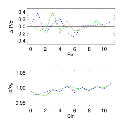
Figure 21: (Top) The change in the the recovered power spectrum relative to the error, after marginalizing over a constant multiplicative bias, for different cosmologies/ prior power spectrum shapes. (Bottom) The ratio of the errors relative to the fiducial case for the same set of cosmologies/ prior power spectra.

A second assumption necessary for the inversion is the choice of a cosmology to convert redshifts to distances. In principle, the consistency between the different slices is a sensitive test of the cosmological model; however, the errors in these data are much larger than this effect. In order to test this, we redo the inversion with 3 different cosmological models, and compare the results in Fig. 21 after marginalizing over the bias. Note that the changes in the power spectrum are significantly smaller than the associated errors, while the errors in the power spectrum remain virtually unchanged. Fig. 21 also demonstrates that the inversion process does not depend on the particular shape of the prior power spectrum.

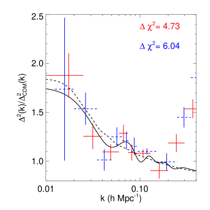
Figure 22: The ratio of the measured power spectrum to the linear CDM power spectrum for our fiducial cosmology (without baryons). As above, the solid and dashed lines represent binnings B1 and B2 respectively. Also shown is the same ratio for the nonlinear prescription, and the “no-wiggle” fit to the power spectrum. The difference in $\chi^{2}$ between these two models is shown for the two binnings. Also note the baryonic suppression of power on large scales, and the rise in power due to nonlinear evolution on small scales

Three important features of this power spectrum are:

• Real space power spectrum : Since the individual angular power spectra make no use of radial information, the 3D power spectrum we obtain is a real space power spectrum on small scales, avoiding the complications of nonlinear redshift space distortions. Note that on length scales much larger than the redshift slice thickness, redshift space distortions cannot be neglected; however, the linear approximation discussed in Sec. 3.1.1 will be valid on these scales.

• Large Scale Power: Fig. 20 shows evidence for power on very large ($k<0.02h{\rm Mpc}^{-1}$) scales. Marginalizing over bands on smaller scales, the significance of the detection on scales $k<0.01h{\rm Mpc}^{-1}$ is $\sim 2\sigma$, increasing to $5.5\sigma$ for $k<0.02h{\rm Mpc}^{-1}$. Note that these scales start to probe the power spectrum at the turnover scale set by matter-radiation equality.

• Baryonic Oscillations: Fig. 22 shows the 3D power spectrum divided by a fiducial linear CDM power spectrum with zero baryonic content. The baryonic suppression of power on large scales, and the rise of power due to nonlinear evolution is clearly seen. We also see evidence for baryonic oscillations on small scales for both binnings, although we note that the power spectrum estimates are anti-correlated, making a visual goodness-of-fit difficult to estimate.

  To estimate the significance of these oscillations, we compare the best fit model obtained in the next section, with a version of the same power spectrum that has the baryonic oscillations edited out (Eisenstein & Hu, 1998). The difference in $\chi^{2}$ for these two models suggests a detection confidence of $\sim 2.5\sigma$ or $\sim 95\%$, assuming approximately Gaussian errors. A similar result is obtained in the next section from cosmological parameter fits to the baryon density.

5 Cosmological Parameters

We defer a complete multi-parameter estimation of cosmological parameters to a later paper, but discuss basic constraints below. We consider a $\Lambda$CDM cosmological model, varying the matter density $\Omega_{M}$ and the baryonic fraction $\Omega_{b}/\Omega_{M}$ and fixing all other parameters to our fiducial choices.

The principal complication to using the galaxy power spectrum for cosmological parameter estimation is understanding the mapping from the linear matter power spectrum to the nonlinear galaxy power spectrum, both due to the nonlinear evolution of structure and scale-dependent bias. We use the fitting formula proposed by Cole et al. (2005),

$$\frac{\Delta^{2}(k)}{\Delta^{2}_{lin}(k)}=b^{2}\frac{1+Qk^{2}}{1+Ak}\,\,,$$ (42)

where $A=1.4$ is appropriate for a real-space power spectrum, and $b$ and $Q$ are two “bias” parameters that we add to the cosmological parameters we estimate. Comparing this parametrization to a red galaxy sample from the Millenium simulations (Springel et al., 2005), shows that this parametrization correctly describes the effects of scale dependent bias and nonlinear evolution up to wavenumbers $k\sim 0.5h{\rm Mpc}^{-1}$ (Volker Springel, private communication). We fit the data to $k=0.3h{\rm Mpc}^{-1}$.

Figure 23: Measurements of $\Omega_{M}$ (upper) and $Q$ (lower) for each of the eight 3D power spectra. The solid lines use binning B1, while the displaced dashed lines use binning B2. Note that $\Omega_{M}$ is insensitive to the redshift slice used, while $Q$ depends sensitively on the particular choice of slice.

A second complication is that the inversion procedure of the previous section only combines wavenumbers $<0.1h{\rm Mpc}^{-1}$; fitting the data beyond this requires choosing one of the eight redshift slices. In order to decide which slice to use, we estimate $\chi^{2}$ on grids varying $\Omega_{M}$, $Q$, and $b$ for each of the eight 3D power spectra. We fix the baryonic density to $\Omega_{b}=0.05$, although allowing it to vary does not change the results.

The best fit values for $\Omega_{M}$ and $Q$ (marginalizing over the other parameters), for each of the eight redshift slices are shown in Fig. 23. We note that $\Omega_{M}$ and its error is insensitive to the choice of redshift slice, although $Q$ depends on the particular redshift slice used. This is due to the fact that $\Omega_{M}$ is constrained by the location of the turnover in the power spectrum, and the shape of the power spectrum in the linear regime, while $Q$ depends on the power spectrum beyond $0.1h{\rm Mpc}^{-1}$. In what follows, we use the redshift slice corresponding to photometric redshifts between 0.45 and 0.50, as it corresponds to the median redshift of the full sample. However, we emphasize that all results below, except for the “nuisance” bias parameters, are insensitive to this particular choice.

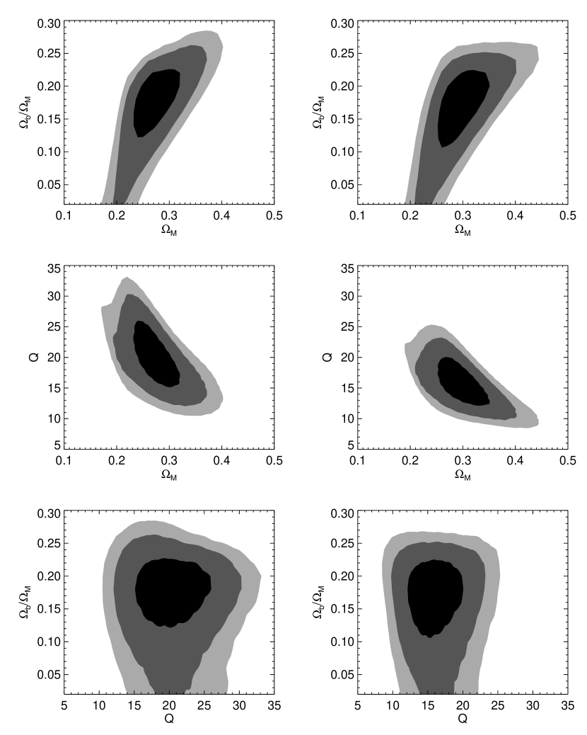
Figure 24: Joint 2D likelihood distributions for $\Omega_{M}$, $Q$ and $\Omega_{b}/\Omega_{m}$, fixing $h=0.7$ and $n=1$, and marginalizing over the galaxy bias. The contours show $\Delta\chi^{2}=2.3,6.17$ and $9.21$. The left column panels use binning B1, while the right column panels use B2. We truncate fitting at $k=0.3h{\rm Mpc}^{-1}$ (using the midpoint of the bins). Note that the two binnings are consistent with each other, with the B2 binning providing slightly tighter constraints.

Fig. 24 shows 2D projections of the $(\Omega_{M},\Omega_{b}/\Omega_{M},Q)$ parameter likelihood space; the multiplicative bias $b$ is marginalized over. The minimum $\chi^{2}$ values are $5.99$ and $6.94$ (bins B1 and B2, respectively), for $5$ and $6$ degrees of freedom, consistent with a reduced $\chi^{2}$ of 1 per degree of freedom. Bins B1 and B2 give consistent values for the cosmological parameters; B2 constrains all parameters (especially $Q$) better than B1 because of the extra binning and the larger $k$ range probed. We note that $Q$ is correlated with $\Omega_{M}$, since both $\Omega_{M}h$ and $Q$ determine the broad shape of the power spectrum. An important consequence of this degeneracy is that an accurate estimation of $\Omega_{M}$ and its error requires varying $Q$; fixing or restricting $Q$ will result in a biased $\Omega_{M}$ and an underestimation of its errors.

Figure 25: The likelihood distributions for $\Omega_{M}$, $Q$ and $\Omega_{b}/\Omega_{M}$. The solid line uses binning B1, while the dashed line uses B2. As in Fig. 24, we truncate at $k=0.3h{\rm Mpc}^{-1}$. Also shown are the best fit values and $1\sigma$ errors for bins B1 (top) and B2 (bottom).

Fig. 25 shows the 1D likelihoods for $(\Omega_{M},\Omega_{b}/\Omega_{M},Q)$, marginalizing over all other parameters; the binnings are again seen to be consistent. The likelihood for $\Omega_{b}/\Omega_{M}$ also allows to estimate the significance of the detection of baryonic features in the power spectrum. The difference in $\chi^{2}$ between the best fit model and the zero-baryon case is $5.75$ and $6.4$ for bins B1 and B2 respectively, suggesting a $2.5\sigma$ detection consistent with the model independent estimates made in the previous section. The significance of this result is similar to the results from the 2dFGRS (Cole et al., 2005), but is weaker than the detection in the spectroscopic LRG sample (Eisenstein et al., 2005b).

Summarizing these results, we have

• For bins B1 :

  $$\Omega_{M}=0.27\pm 0.03$$

  $$\Omega_{b}/\Omega_{M}=0.18\pm 0.03$$

  $$Q=20.3\pm 3.6$$ (43)

• For bins B2 :

  $$\Omega_{M}=0.30\pm 0.03$$

  $$\Omega_{b}/\Omega_{M}=0.18\pm 0.04$$

  $$Q=15.6\pm 2.6$$ (44)

In light of the recent WMAP results (Spergel et al., 2006), it is interesting to understand how the above reults change if we deviate from a scale-invariant primordial spectrum. Minimizing $\chi^{2}$ over $\Omega_{M}$, $\Omega_{b}/\Omega_{M}$, and $Q$ assuming $n=0.95$, we find that (for bins B2),

$$\Omega_{M}=0.31\pm 0.03$$

$$\Omega_{b}/\Omega_{M}=0.16\pm 0.04$$

$$Q=16.3\pm 2.8\,\,.$$ (45)

Reducing $n$ (while keeping $\sigma_{8}$ fixed) boosts the power on large scales, but suppresses it on small scales. This results in a better fit on large scales, and a worse fit on small scales. To compensate for this, the best fit value of $\Omega_{b}/\Omega_{M}$ decreases (reducing Silk damping) while $Q$ increases, boosting the power back up on small scales, while leaving the large scale power spectrum unchanged. The minimum $\chi^{2}$ is marginally worse ($7.24$) than the scale invariant case. Note however that all the parameters are within the 1-$\sigma$ errors of those obtained assuming scale invariance.

5.1 Distance to $z=0.5$

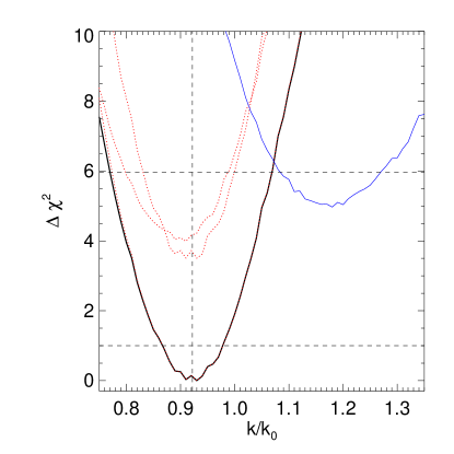
Figure 26: The solid line shows the likelihood of the ratio of the fiducial distance to $z=0.5$ to the observed distance $k/k_{0}$, marginalizing over $Q$ and the galaxy bias, but fixing $\Omega_{b}h^{2}=0.0223$, $\Omega_{M}h^{2}=0.127$ and $Q=15.6$. The dotted lines show slices through the 2D likelihood distribution of $Q$ and $k/k_{0}$ at $Q=16.5$, $19.5$ and $22.5$ (from left to right). Note that the $Q$ and $k/k_{0}$ are approximately orthogonal directions; varying the nonlinear correction doesn’t change the distance scale. The best fit value of $0.92\pm 0.06$ is shown by the dashed lines. The thin solid line shows the $k/k_{0}$ likelihood for a negligible baryonic fraction; the distance constraint degrades to a $10\%$ measurement.

A potential application of the galaxy power spectrum is as a standard ruler. The two features of interest, the turnover and the baryon oscillations are determined by the physical baryon and matter densities - $\Omega_{b}h^{2}$ and $\Omega_{M}h^{2}$. Both of these are precisely determined by the peak structure of the CMB power spectrum. Therefore, in order to understand the sensitivity of the current measurements as standard rulers, we fix $\Omega_{b}h^{2}=0.0223$ and $\Omega_{M}h^{2}=0.127$, and vary $Q$ and the comoving distance. In general, one would need to vary the comoving distance to each of the 8 redshift slices and recompute the power spectrum. However, given the S/N of the baryonic oscillations and turnover in these data, we simply translate the 3D power spectrum in $k$ with reference to our fiducial cosmology at the median redshift of the slice $k_{0}$. The likelihood is in Fig. 26; these data can constrain the distance to $z=0.5$ to $6\%$. Note that this is for a fixed value of $\Omega_{M}h^{2}$. Assuming a $10\%$ uncertainty in $\Omega_{M}h^{2}$ from current CMB measurements results in a $\sim 2.5\%$ uncertainty in the sound horizon, increasing the distance error to $6.5\%$. This must be compared to the $5\%$ measurement of the distance to $z\sim 0.35$ measured by the spectroscopic LRG sample.

Equally interesting is that $Q$ and $k/k_{0}$ are orthogonal; the distance measurement does not change for different values of the nonlinear correction. This highlights an important property of baryon oscillations as a distance measurement - it is relatively insensitive to the nonlinearity corrections that affect the galaxy power spectrum.

We would also like to understand the fraction of the distance constraint from baryonic oscillations as opposed to the power spectrum shape. Fig. 26 also shows the likelihood for a model with a negligible baryonic fraction; the distance accuracy degrades to $10\%$, suggesting that most of the constraint comes from the oscillations.

6 Discussion

6.1 Principal Results

We have measured the 3D clustering power spectrum of luminous red galaxies using the SDSS photometric survey. The principal results of this analysis are summarized below.

• Photometric redshifts: This analysis demonstrates the feasibility of using multi-band imaging surveys with well calibrated photometric redshifts as a probe of the large scale structure of the Universe. Accurate photometric redshifts are critical to being able to narrow the range of physical scales that correspond to the clustering on a particular angular scale, and thereby estimate the 3D power spectrum.

• Largest cosmological volume: Using photometric redshifts allowed us to construct a uniform sample of galaxies between redshifts $z=0.2$ to $0.6$. This probes a cosmological volume of $\sim 1.5h^{-3}{\rm Gpc}^{3}$, making this the largest cosmological volume ever used for a galaxy clustering measurement. The large volume allows us to measure power on very large scales, yielding a $\sim 2\sigma$ detection of power for $k<0.01h{\rm Mpc}$, increasing in significance to $\sim 5.5\sigma$ for $k<0.02h{\rm Mpc}$.

• Real Space Power Spectrum: This power spectrum is intrinsically a real space power spectrum, and is unaffected by redshift space distortions on scales $k>0.01h{\rm Mpc}^{-1}$. This obviates any need to model redshift space distortions in the quasi-linear regime, allowing for a more direct comparison to theoretical predictions.

• Baryonic Oscillations: The 3D power spectrum shows evidence for baryonic oscillations at the $\sim 2.5\sigma$ confidence level, both in the shape of the 3D power spectrum, as well as fits of the baryonic density. We emphasize that this is only possible in the stacked 3D power spectrum, and therefore relies on accurate photometric redshift distributions.

• Cosmological Parameters: The large volume and small statistical errors of these data constrain both the normalization and scale dependence of the galaxy bias. Using a functional form for the scale dependence of the bias motivated by N-body simulations, we fit for the matter density and baryonic fraction jointly, and obtain $\Omega_{M}=0.30\pm 0.03$ and $\Omega_{b}/\Omega_{M}=0.18\pm 0.03$.

6.2 Using these results

For cosmological parameter analyses, we recommend directly using the 3D power spectra (binning B2), fitting both the galaxy bias ($b$) and its scale-dependence ($Q$) to $k=0.3h{\rm Mpc}^{-1}$. Electronic versions of all the power spectra, and covariance matrices used in this paper will be made publically available. In addition, a simple FORTRAN subroutine that returns $\chi^{2}$ given an input power spectrum will also be made public.

6.3 Comparison with other results

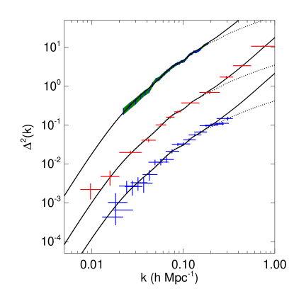
Figure 27: Comparison between power spectra from the SDSS MAIN spectroscopic survey (bottom), 2dFGRS $P(k)$ (top), and the photometric SDSS LRGs (binning B2) from this work (middle). The normalizations are arbitrary, and have been simply chosen to separate the three power spectra. Adjacent LRG $P(k)$ errors are anticorrelated, while the 2dFGRS errors are strongly correlated. The dotted line shows the linear power spectrum for our fiducial cosmology, whereas the solid line is the halofit presciption for the nonlinear power spectrum. Note that the LRG power spectrum fits the nonlinear power spectrum to $k\sim 1h{\rm Mpc}^{-1}$.

Fig. 27 compares the LRG power spectrum (B2 binning), with the power spectrum obtained from the SDSS MAIN spectroscopic survey (Tegmark et al., 2004) and the 2dFGRS (Cole et al., 2005); these three samples will be referred to as LRG, MAIN, and 2dF throughout this section. The solid and dotted lines show our nonlinear and linear fiducial power spectrum. Note that the normalization is arbitrary, and that we have not attempted to deconvolve the 2dF window function.

The two principal differences between these surveys and the data presented here is the volume probed, and the density of objects. As both the MAIN and 2dF are at low redshifts (median $z\sim 0.1$),  the volume probed is $<0.05h^{-3}{\rm Gpc}^{3}$, whereas our sample probes $1.5h^{-3}{\rm Gpc}^{3}$ (at a median redshift of $z\sim 0.5$) allowing us to measure the largest scales with smaller statistical errors, even with crude redshift estimates. This is clearly evident from Fig. 27, where the LRG power spectrum extends to smaller $k$ than either of the other two power spectra.

On small scales, we again emphasize that the LRG power spectrum is naturally a real space power spectrum, and is unaffected by redshift space distortions. By contrast, the 2dF $P(k)$ is in redshift space, and the MAIN $P(k)$ which involves attempting to correct for linear redshift space distortions. Note that the SDSS $P(k)$ falls below the nonlinear power spectrum at $k\sim 0.3h{\rm Mpc}^{-1}$, in line with the simulation results of Tegmark et al. (2004) that motivated the discarding of $k>0.2h{\rm Mpc}^{-1}$ data from the cosmological parameter analysis. This is a manifestation of nonlinear redshift distortions, which are particularly important given recent results that suggest that redshift distortions go nonlinear on larger scales than previously anticipated (Slosar et al., 2006).

Survey	$\Omega_{M}$
SDSS MAIN	$0.297\,(+0.0219,-0.0196)$
2dFGRS	$0.271\,(+0.021,-0.0187)$
SDSS LRG (B1)	$0.260\,(+0.0111,-0.0102)$
SDSS LRG (B2)	$0.286\,(+0.0119,-0.0111)$

Table 4: The best fit values for $\Omega_{M}$ assuming $\Omega_{b}h^{2}=0.024$, $h=0.72$ and a scale invariant initial perturbation spectrum. We use the best fit nonlinear prescription suggested by the respective authors to fit the power spectrum to $k=0.2h{\rm Mpc}^{-1}$. The numbers in parentheses are the upper and lower $1-\sigma$ errors.

Each of the three power spectra are consistent with the overall shape of the fiducial power spectrum, suggesting that they are consistent with each other. In order to make this precise and to compare statistical power, we fit for $\Omega_{M}$ and the galaxy bias assuming $\Omega_{b}h^{2}=0.024$, $h=0.72$ and a scale invariant initial perturbation spectrum. To ensure a fair comparison, we fit all power spectra to $k=0.2h{\rm Mpc}^{-1}$ using the best fit prescription for nonlinearity suggested by the authors. The results are summarized in Table 4; we find that all three power spectra yield consistent values for $\Omega_{M}$. The LRG power spectrum, however, reduces the error by a factor of $\sim 1.75$ compared with previous results.

On the other hand, the SDSS LRG spectroscopic sample is similar to this sample. The effective spectroscopic LRG volume is $0.75h^{-3}{\rm Gpc}^{3}$ at a median redshift of $z\sim 0.35$. However, the spectroscopic LRGs are sparser, with shot noise responsible for approximately half the statistical error on all scales. One can compare the S/N of the two samples as follows - since we are only using auto-correlations of the redshift slices and are ignoring correlations between different redshift slices, we are losing a factor $\sim 7$ in the number of modes (most of the remaining cosmological information is contained in adjacent redshift slices). We however gain a factor $\sim 2$ from the increased volume, and another factor $\sim 2$ from the higher spatial density of objects, suggesting that the SDSS spectroscopic LRG sample would be a factor of $\sim 2$ greater in S/N than the photometric sample. This is borne out by the fact that the spectroscopic sample detects baryonic oscillations with $\Delta\chi^{2}=11.7$, while the photometric sample has $\Delta\chi^{2}=6.04$, about a factor of $2$ smaller. Note that this analysis breaks down both on the largest scales (where the photometric survey has more leverage because of the greater volume), and on scales smaller than the redshift errors (where the spectroscopic sample resolves more modes). In principle, one could gain further by using the cross correlations between different redshift slices. However, as seen in Fig. 18, this is very sensitive to errors in the tails of the redshift distribution.

We can also compare our cosmological results with those obtained from the third year CMB temperature and polarization measurements from the WMAP satellite (Spergel et al., 2006). The WMAP error on $\Omega_{M}$ is dominated by the error on the Hubble constant; they obtain $\Omega_{M}=0.26^{+0.01}_{-0.03}$, compared with our estimate of $\Omega_{M}=0.30\pm 0.03$. They also obtain $\Omega_{b}/\Omega_{M}=0.17$, compared with $\Omega_{b}/\Omega_{M}=0.18\pm 0.04$. Note that WMAP favours a primordial scalar spectral index of $n\sim 0.94$; using this instead of scale invariance reduces our estimate of $\Omega_{b}/\Omega_{M}$ to $0.16\pm 0.04$, while increasing $\Omega_{M}=0.31\pm 0.03$. We also emphasize that the errors are not directly comparable, since our analysis uses stricter priors. It is, however, important and encouraging to note that we obtain consistent results with a completely independent dataset.

6.4 Future Directions

We conclude with a discussion of the future prospects for photometric surveys. As of this writing, the SDSS has imaged twice the area used in this paper, potentially reducing the errors by a factor of $\sqrt{2}$. In addition, there are a number of imaging surveys planned for the near and distant future, the Pan-STARRS and LSST being two notable examples. Both of these surveys will ultimately cover about three times the final SDSS area to a much greater depth, further increasing the volume probed.

Baryonic oscillations are also now emerging as an important tool to constrain the properties of dark energy. The tradeoff between photometric and spectroscopic approaches to their measurement is simple - photometric surveys require wide field ($>10,000{\rm deg}^{2}$) multi-band imaging surveys, whereas spectroscopic surveys require large multi-object spectrographs. Both of these approaches are being actively developed, and the prudent approach would be to pursue both, using the results from one to inform the other. It is worth emphasizing that wide-field imaging surveys are an essential prerequisite for the other approaches (with very different systematic errors) to understanding dark energy, namely supernovae and weak lensing, suggesting a synergy between these techniques.

Given the efforts underway to plan the next generation of surveys, it is timely to compare the precision of the distance measurement we obtain with the fitting formulae of Blake et al. (2006). Substituting our survey parameters into their photometric fitting formula, assuming a median redshift of $z\sim 0.5$ and a photometric redshift error $\sigma_{z}\sim 100h^{-1}{\rm Mpc}$ (corresponding to the redshift error at $z\sim 0.5$), we estimate a distance error of $7\%$ as compared with the actual $6\%$ error obtained. Note that Blake et al. (2006) only use the oscillation to determine the distance, whereas we use the entire power spectrum.

We can now estimate the potential sensitivity of the next generation of surveys. Assuming a straw-man survey of $20,000{\rm deg}^{2}$ with a median redshift of $z\sim 0.8$, and photometric redshift errors of $\sim 50h^{-1}{\rm Mpc}$, we find a factor of $\sim 5$ improvement in the distance measurement, yielding a $\sim 1\%$ measurement, the current benchmark for dark energy surveys. Note that this is a conservative estimate, since the photometric redshift accuracies assumed have already been achieved with the SDSS.

In order to do so, there are a number of challenges that must be overcome, in addition to the brute force observational effort required. The first is technical - this work relied heavily on having accurate, well calibrated photometric redshifts. Demonstrating that this is possible at higher redshifts, and calibrating the redshift errors is essential. The second challenge is theoretical - in order to optimally use galaxy clustering for cosmology, we will now need to understand the connections between the physics of galaxy formation and the observed clustering of galaxies. The hope is that the interplay between the two would result in a more complete cosmological model.

We thank Lloyd Knox, Eric Linder, Yeong Loh, Taka Matsubara, David Weinberg and Martin White for useful discussions. We also thank the 2SLAQ collaboration for measuring the spectroscopic redshifts used to calibrate the photometric redshift algorithm.

Funding for the SDSS and SDSS-II has been provided by the Alfred P. Sloan Foundation, the Participating Institutions, the National Science Foundation, the U.S. Department of Energy, the National Aeronautics and Space Administration, the Japanese Monbukagakusho, the Max Planck Society, and the Higher Education Funding Council for England. The SDSS Web Site is http://www.sdss.org/.

The SDSS is managed by the Astrophysical Research Consortium for the Participating Institutions. The Participating Institutions are the American Museum of Natural History, Astrophysical Institute Potsdam, University of Basel, Cambridge University, Case Western Reserve University, University of Chicago, Drexel University, Fermilab, the Institute for Advanced Study, the Japan Participation Group, Johns Hopkins University, the Joint Institute for Nuclear Astrophysics, the Kavli Institute for Particle Astrophysics and Cosmology, the Korean Scientist Group, the Chinese Academy of Sciences (LAMOST), Los Alamos National Laboratory, the Max-Planck-Institute for Astronomy (MPIA), the Max-Planck-Institute for Astrophysics (MPA), New Mexico State University, Ohio State University, University of Pittsburgh, University of Portsmouth, Princeton University, the United States Naval Observatory, and the University of Washington.

The 2SLAQ Redshift Survey was made possible through the dedicated efforts of the staff at the Anglo-Australian Observatory, both in creating the 2dF instrument and supporting it on the telescope.

References

- Abazajian et al. (2005) Abazajian K. et al., 2005, AJ, 129, 1755
- Abazajian et al. (2004) Abazajian K. et al., 2004, AJ, 128, 502
- Abazajian et al. (2003) Abazajian K. et al., 2003, AJ, 126, 2081
- Adelman-McCarthy et al. (2006) Adelman-McCarthy J. K. et al., 2006, ApJS, 162, 38
- Blake & Bridle (2005) Blake C., Bridle S., 2005, MNRAS, 363, 1329
- Blake & Glazebrook (2003) Blake C., Glazebrook K., 2003, ApJ, 594, 665
- Blake et al. (2006) Blake C., Parkinson D., Bassett B., Glazebrook K., Kunz M., Nichol R. C., 2006, MNRAS, 365, 255
- Blanton et al. (2003) Blanton M. R., Lin H., Lupton R. H., Maley F. M., Young N., Zehavi I., Loveday J., 2003, AJ, 125, 2276
- Blanton et al. (2005) Blanton M. R. et al., 2005, AJ, 129, 2562
- Bond & Efstathiou (1984) Bond J. R., Efstathiou G., 1984, ApJ, 285, L45
- Bruzual & Charlot (2003) Bruzual G., Charlot S., 2003, MNRAS, 344, 1000
- Cole et al. (2005) Cole S. et al., 2005, MNRAS, 362, 505
- Dolney et al. (2006) Dolney D., Jain B., Takada M., 2006, MNRAS, 366, 884
- Eisenstein (2005) Eisenstein D. J., 2005, New Astronomy Review, 49, 360
- Eisenstein et al. (2001) Eisenstein D. J. et al., 2001, AJ, 122, 2267
- Eisenstein et al. (2005a) Eisenstein D. J., Blanton M., Zehavi I., Bahcall N., Brinkmann J., Loveday J., Meiksin A., Schneider D., 2005a, ApJ, 619, 178
- Eisenstein & Hu (1998) Eisenstein D. J., Hu W., 1998, ApJ, 496, 605
- Eisenstein et al. (1998) Eisenstein D. J., Hu W., Tegmark M., 1998, ApJ, 504, L57
- Eisenstein et al. (1999) Eisenstein D. J., Hu W., Tegmark M., 1999, ApJ, 518, 2
- Eisenstein & Zaldarriaga (2001) Eisenstein D. J., Zaldarriaga M., 2001, ApJ, 546, 2
- Eisenstein et al. (2005b) Eisenstein D. J. et al., 2005b, ApJ, 633, 560
- Finkbeiner et al. (2004) Finkbeiner D. P. et al., 2004, AJ, 128, 2577
- Fisher et al. (1994) Fisher K. B., Scharf C. A., Lahav O., 1994, MNRAS, 266, 219
- Fukugita et al. (1996) Fukugita M., Ichikawa T., Gunn J. E., Doi M., Shimasaku K., Schneider D. P., 1996, AJ, 111, 1748
- Gladders & Yee (2000) Gladders M. D., Yee H. K. C., 2000, AJ, 120, 2148
- Goldberg & Strauss (1998) Goldberg D. M., Strauss M. A., 1998, ApJ, 495, 29
- Górski et al. (1999) Górski K. M., Hivon E., Wandelt B. D., 1999, in Evolution of Large Scale Structure : From Recombination to Garching, p. 37
- Groth & Peebles (1977) Groth E. J., Peebles P. J. E., 1977, ApJ, 217, 385
- Gunn et al. (1998) Gunn J. E. et al., 1998, AJ, 116, 3040
- Gunn et al. (2006) Gunn J. E. et al., 2006, AJ, 131, 2332
- Hauser & Peebles (1973) Hauser M. G., Peebles P. J. E., 1973, ApJ, 185, 757
- Hirata et al. (2004) Hirata C. M., Padmanabhan N., Seljak U., Schlegel D., Brinkmann J., 2004, Phys. Rev. D, 70, 103501
- Høg et al. (2000) Høg E. et al., 2000, A&A, 355, L27
- Hogg et al. (2001) Hogg D. W., Finkbeiner D. P., Schlegel D. J., Gunn J. E., 2001, AJ, 122, 2129
- Holtzman (1989) Holtzman J. A., 1989, ApJS, 71, 1
- Hu (2005) Hu W., 2005, in Wolff S. C., Lauer T. R., ed, ASP Conf. Ser. 339: Observing Dark Energy, p. 215
- Hu et al. (1998) Hu W., Eisenstein D. J., Tegmark M., 1998, Physical Review Letters, 80, 5255
- Hu et al. (1999) Hu W., Eisenstein D. J., Tegmark M., White M., 1999, Phys. Rev. D, 59, 023512
- Hu & Haiman (2003) Hu W., Haiman Z., 2003, Phys. Rev. D, 68, 063004
- Huterer et al. (2001) Huterer D., Knox L., Nichol R. C., 2001, ApJ, 555, 547
- Hütsi (2006) Hütsi G., 2006, A&A, 449, 891
- Ivezić et al. (2004) Ivezić Ž. et al., 2004, Astronomische Nachrichten, 325, 583
- Kaiser (1987) Kaiser N., 1987, MNRAS, 227, 1
- Kendall & Stuart (1977) Kendall M., Stuart A., 1977, The advanced theory of statistics. Vol.1: Distribution theory. London: Griffin, 1977, 4th ed.
- Linder (2003) Linder E. V., 2003, Phys. Rev. D, 68, 083504
- Lupton et al. (2001) Lupton R. H., Gunn J. E., Ivezić Z., Knapp G. R., Kent S., Yasuda N., 2001, in ASP Conf. Ser. 238: Astronomical Data Analysis Software and Systems X, p. 269
- Matsubara (2004) Matsubara T., 2004, ApJ, 615, 573
- Matsubara & Szalay (2003) Matsubara T., Szalay A. S., 2003, Physical Review Letters, 90, 021302
- Meiksin et al. (1999) Meiksin A., White M., Peacock J. A., 1999, MNRAS, 304, 851
- Padmanabhan et al. (2005a) Padmanabhan N. et al., 2005a, MNRAS, 359, 237
- Padmanabhan et al. (2005b) Padmanabhan N., Hirata C. M., Seljak U., Schlegel D. J., Brinkmann J., Schneider D. P., 2005b, Phys. Rev. D, 72, 043525
- Padmanabhan et al. (2003) Padmanabhan N., Seljak U., Pen U. L., 2003, New Astronomy, 8, 581
- Padmanabhan et al. (2001) Padmanabhan N., Tegmark M., Hamilton A. J. S., 2001, ApJ, 550, 52
- Peebles (1973) Peebles P. J. E., 1973, ApJ, 185, 413
- Peebles & Yu (1970) Peebles P. J. E., Yu J. T., 1970, ApJ, 162, 815
- Pier et al. (2003) Pier J. R., Munn J. A., Hindsley R. B., Hennessy G. S., Kent S. M., Lupton R. H., Ivezić Ž., 2003, AJ, 125, 1559
- Press et al. (1992) Press W. H., Teukolsky S. A., Vetterling W. T., Flannery B. P., 1992, Numerical recipes in FORTRAN. The art of scientific computing. Cambridge University Press, 1992, 2nd ed.
- Richards et al. (2002) Richards G. T. et al., 2002, AJ, 123, 2945
- Scherrer & Weinberg (1998) Scherrer R. J., Weinberg D. H., 1998, ApJ, 504, 607
- Schlegel et al. (1998) Schlegel D. J., Finkbeiner D. P., Davis M., 1998, ApJ, 500, 525
- Seljak (1998) Seljak U., 1998, ApJ, 506, 64
- Seo & Eisenstein (2003) Seo H., Eisenstein D. J., 2003, ApJ, 598, 720
- Seo & Eisenstein (2005) Seo H.-J., Eisenstein D. J., 2005, ApJ, 633, 575
- Slosar et al. (2006) Slosar A., Seljak U., Tasitsiomi A., 2006, MNRAS, 366, 1455
- Smith et al. (2002) Smith J. A. et al., 2002, AJ, 123, 2121
- Smith et al. (2003) Smith R. E. et al., 2003, MNRAS, 341, 1311
- Spergel et al. (2006) Spergel D. N. et al., 2006, ApJ submitted (astro-ph/0603449)
- Springel et al. (2005) Springel V. et al., 2005, Nature, 435, 629
- Stoughton et al. (2002) Stoughton C., Lupton R. H., Bernardi M., Blanton M. R., et al , 2002, AJ, 123, 485
- Strauss et al. (2002) Strauss M. A. et al., 2002, AJ, 124, 1810
- Sunyaev & Zeldovich (1980) Sunyaev R. A., Zeldovich I. B., 1980, ARA&A, 18, 537
- Tegmark (1997a) Tegmark M., 1997a, ApJ, 480, L87
- Tegmark (1997b) Tegmark M., 1997b, Physical Review Letters, 79, 3806
- Tegmark et al. (2004) Tegmark M. et al., 2004, ApJ, 606, 702
- Tegmark et al. (2002) Tegmark M. et al., 2002, ApJ, 571, 191
- Tegmark et al. (1998) Tegmark M., Hamilton A. J. S., Strauss M. A., Vogeley M. S., Szalay A. S., 1998, ApJ, 499, 555
- Wang et al. (1999) Wang Y., Spergel D. N., Strauss M. A., 1999, ApJ, 510, 20
- White (2005) White M., 2005, Astroparticle Physics, 24, 334
- York et al. (2000) York D. G. et al., 2000, AJ, 120, 1579
- Zehavi et al. (2005) Zehavi I. et al., 2005, ApJ, 621, 22