Physical viscosity in smoothed particle hydrodynamics simulations of galaxy clusters

Abstract

Most hydrodynamical simulations of galaxy cluster formation carried out to date have tried to model the cosmic gas as an ideal, inviscid fluid, where only a small amount of (unwanted) numerical viscosity is present, arising from practical limitations of the numerical method employed, and with a strength that depends on numerical resolution. However, the physical viscosity of the gas in hot galaxy clusters may in fact not be negligible, suggesting that a self-consistent treatment that accounts for the internal gas friction would be more appropriate. To allow such simulations using the smoothed particle hydrodynamics (SPH) method, we derive a novel SPH formulation of the Navier-Stokes and general heat transfer equations and implement them in the GADGET-2 code. We include both shear and bulk viscosity stress tensors, as well as saturation criteria that limit viscous stress transport where appropriate. Our scheme integrates consistently into the entropy and energy conserving formulation of SPH employed by the code. Using a number of simple hydrodynamical test problems, e.g. the flow of a viscous fluid through a pipe, we demonstrate the validity of our implementation. Adopting Braginskii parameterization for the shear viscosity of hot gaseous plasmas, we then study the influence of viscosity on the interplay between AGN–inflated bubbles and the surrounding intracluster medium (ICM). We find that certain bubble properties like morphology, maximum clustercentric radius reached, or survival time depend quite sensitively on the assumed level of viscosity. Interestingly, the sound waves launched into the ICM by the bubble injection are damped by physical viscosity, establishing a non-local heating process. However, we find that the associated heating is rather weak due to the overall small energy content of the sound waves. Finally, we carry out cosmological simulations of galaxy cluster formation with a viscous intracluster medium. We find that the presence of physical viscosity induces new modes of entropy generation, including a significant production of entropy in filamentary regions perpendicular to the direction of the clusters encounter. Viscosity also modifies the dynamics of mergers and the motion of substructures through the cluster atmosphere. Substructures are generally more efficiently stripped of their gas, leading to prominent long gaseous tails behind infalling massive halos.

1 Introduction

Studies of the intracluster medium (ICM) provide unique information about the complex interplay of the physical processes that determine the fate of baryons in galaxy groups and clusters. In recent years, remarkable observational progress has in fact unveiled a completely revised picture of the intracluster medium (ICM) where a plethora of non-gravitational physical processes are responsible for key observational phenomena. Indeed, the list of recent discoveries in the field of ICM physics is quite long, and includes cold fronts, long X-ray tails in the wake of late type galaxies passing through the hot cluster environment, or the presence of radio halos and ghosts associated with past AGN activity. Theoretical studies of these phenomena increasingly rely on direct numerical simulations, which are in principle capable of accurately computing the non-linear interplay of all these processes and their consequences for the thermodynamics of the ICM. A prerequisite is that the simulations are capable of representing all the physics relevant for the system, which represents a significant ongoing challenge.

A particularly important question in cluster physics concerns the observed absence of strong cooling flows onto the massive elliptical galaxies at the centres of the potential wells of groups and clusters of galaxies (e.g. Peterson et al., 2001, 2003; Tamura et al., 2001; Balogh et al., 2001; Edge, 2001; Edge et al., 2002; Böhringer et al., 2002). There is now growing observational evidence for the relevance of AGN heating in these objects (e.g. McNamara et al., 2000; Sanders & Fabian, 2002; Mazzotta et al., 2002; McNamara et al., 2005; Fabian et al., 2006), supporting the widespread theoretical notion that the central AGN is providing enough energy to offset the radiative cooling losses. However, it is still not understood in detail how this energy is coupled into the ICM. X-ray observations with the XMM-Newton and Chandra telescopes (e.g. Blanton et al., 2001; Bîrzan et al., 2004; Nulsen et al., 2005) have revealed that in many cooling-flow clusters there are so called X-ray cavities which interact with the surrounding intracluster gas. It is believed that these bubbles are inflated by the powerful AGN jets that are generated by an accreting central black hole. The expanding bubbles heat the ICM by mechanical work, and by the buoyant uplifting of cool gas from the central regions and subsequent mixing with the hotter atmosphere at larger radii. At the same time, the bubbles trigger sound waves that travel through the cluster, and they may excite global oscillations modes of the ICM in the cluster potential. It has been suggested that viscous damping of these sound waves may provide an important non-local heating source for the ICM (e.g. Fabian et al., 2003). A significant cluster viscosity may in principle exist, but its strength should depend critically on the magnetic field strength and the field topology.

Radio observations (e.g. Owen et al., 2000; Clarke et al., 2005; Dunn et al., 2005) have clearly shown that the X-ray cavities are filled with relativistic gas, and probably have inherited some of the magnetic fields transported by the AGN jet. While the structure of the magnetic fields filling the bubbles is not well known yet, it has by now been firmly established that galaxy clusters are permeated by magnetic fields (for reviews see Carilli & Taylor, 2002; Govoni & Feretti, 2004). Faraday rotation measurements (Clarke et al., 2001; Clarke, 2004; Eilek & Owen, 2002; Vogt & Enßlin, 2003, 2005) have found that the magnetic fields in clusters appear to be random, with an rms strength of order of $1-10\,\mu{\rm G}$, and with a coherence length of $1-20\,{\rm kpc}$. Assuming a fully ionized plasma (Spitzer, 1962), this implies a very high magnetic Prandtl number for the ICM of order of $\sim 10^{29}$, suggesting that magneto-hydrodynamic (MHD) turbulence is probably relevant. On the other hand, the inferred typical Reynolds numbers for the intracluster gas are quite small, $\lower 3.22916pt\hbox{$\sim$}\hbox to0.0pt{\hss\raise 1.1625pt\hbox{$<$}}100$, indicating that the gas viscosity might be quite important. Moreover, the coherence length-scale of the magnetic fields is comparable to the ion mean free path, as well as to the typical size of galaxies and of AGN–driven bubbles that could drive turbulence in the ICM. In fact, there have been some observational studies that found evidence for the presence of turbulence in clusters (Schuecker et al., 2004; Rebusco et al., 2005), suggesting that the injection scale of the turbulence would be of order $\sim 10-100\,{\rm kpc}$.

All these observational pieces of information do not yet combine to a definitive picture of the magnetic and viscous properties of the ICM, and the theoretical understanding is also not yet mature (for a recent review see Schekochihin & Cowley, 2005). It is clear, however, that an approximation of the ICM as an ideal, inviscid gas – as usually made in most hydrodynamical simulations of galaxy cluster formation – may be a poor approximation for hot clusters with non-negligible (and perhaps chaotically tangled) magnetic fields. It is therefore the aim of this work to explore the potential imprints of gas viscosity on galaxy cluster properties in a fully self-consistent way, using cosmological simulations of cluster growth from $\Lambda$CDM initial conditions. As a prerequisite for such simulations, we develop a numerical scheme capable of accurately solving the Navier-Stokes equations in SPH, which we use instead of the commonly employed much simpler Euler equation. We will assume a simple parameterization of the shear and bulk viscosity tensors, without explicitly dealing with the MHD equations. For this purpose, we adopt Braginskii parameterization (Braginskii, 1958, 1965) of the shear viscosity, together with a phenomenological suppression factor to mimic the influence of the magnetic fields. The bulk viscosity coefficient is kept constant if included.

In order to test our new hydrodynamical scheme, we apply it to a number of simple test problems with known analytic solutions. These tests yield robust results in agreement with the expectations. We then carry out simulations of galaxy clusters where we include different physics, with or without physical viscosity. These simulations include models with non-radiative hydrodynamics, and models with radiative cooling, star formation and supernovae (SNe) feedback, allowing us to obtain an overview about the interplay of gas dynamics and viscous dissipation in different environments, and the consequences viscosity has for the structure of clusters. We also try to identify potential observational signatures for internal friction processes.

In an additional set of simulations, we analyze the impact of gas viscosity on the AGN–driven bubble heating process. Previous analytic work (e.g. Kaiser et al., 2005) and numerical Eulerian simulations (e.g. Ruszkowski et al., 2004; Reynolds et al., 2005) have suggested that internal friction has a significant impact on bubble properties, stabilizing them against hydrodynamical instabilities that would otherwise readily disrupt them. We explore this issue in some detail with our simulation methodology, in particular studying bubble morphologies, maximum clustercentric distance, and survival times, as a function of the assumed level of shear viscosity. In this context we also examine the total energy in the sound waves triggered by the bubbles. We find that this is rather small, something that could in part be caused by deficiencies in our models, as we discuss later on.

The outline of this paper is as follows. In Section 2, we review the fundamental physical laws of viscous fluids, focusing in particular on astrophysical plasmas and a discussion of the role of magnetic fields. The detailed description of our numerical implementation of physical viscosity in SPH is given in Section 3, while we illustrate the validity of our numerical scheme with a number of basic hydrodynamical test problems in Section 4. In Section 5, we analyze the heating effects caused by AGN–driven bubbles rising through viscous intracluster gas, while in Section 6, we discuss internal friction during merging episodes and its impact on substructure motion in cosmological simulations of galaxy cluster formation. Finally, we summarize and discuss our results in Section 7.

2 Theoretical considerations

In the following discussion, we concentrate on viscous gases in the astrophysical context of galaxy and galaxy cluster formation. We briefly review the basic physical equations governing the hydrodynamics of the relevant class of ‘real’ (as opposed to ideal) fluids, and the constraints that exist for some of the free parameters that describe their properties. This includes a discussion of internal friction processes in the collisional regime and their relevance for astrophysical plasmas. In particular, we examine viscous effects in intracluster gas, assuming that it is fully ionized and that it consists of a primordial mixture of hydrogen and helium. We also describe the differences and difficulties that arise when magnetic fields are present in clusters.

2.1 Navier-Stokes equation

To describe real fluids, two of the fundamental equations of hydrodynamics that hold for ideal gases, namely Euler’s equation and the energy conservation law, need to be revised. The continuity equation remains in its familiar form, i.e.

$$\frac{\partial\rho}{\partial t}+\frac{\partial(\rho v_{k})}{\partial x_{k}}\,=\,0$$ (1)

expresses mass conservation as usual, where $\rho$ is the gas density, $v_{k}$ denotes the local velocity vector of the fluid, and the summation convention has been employed.

When there is relative motion between different parts of a real fluid, internal friction forces lead to an additional transfer of momentum that is absent in an ideal gas, and which in general will act to reduce velocity differences. The friction forces modify the momentum flux density tensor, which becomes

$$\Pi_{ik}\,=\,p\delta_{ik}+\rho v_{i}v_{k}-\sigma_{ik}\,.$$ (2)

In this equation, $p$ is the gas pressure and $\sigma_{ik}$ represents the viscous stress tensor, which to first approximation can be assumed to be a linear function of the first spatial derivatives of the velocity field. It can be shown (Landau & Lifshitz, 1987) that the most general tensor of rank two satisfying the requested criterion is given by

$$\sigma_{ik}\,=\,\eta\bigg{(}\frac{\partial v_{i}}{\partial x_{k}}+\frac{\partial v_{k}}{\partial x_{i}}-\frac{2}{3}\delta_{ik}\frac{\partial v_{l}}{\partial x_{l}}\bigg{)}+\zeta\delta_{ik}\frac{\partial v_{l}}{\partial x_{l}}\,,$$ (3)

where $\eta$ is called the coefficient of shear viscosity, and $\zeta$ represents the bulk viscosity coefficient. Bulk viscosity becomes important when the fluid is rapidly compressed or expanded on a timescale shorter than the relaxation time of the fluid, in which case considerable energy can be dissipated. The coefficients of viscosity can be functions both of gas pressure and temperature, but not of gas velocity, because of the criterion imposed above on the viscous stress tensor.

The generalized form of Euler’s equation describing the motion of viscous fluids can be written as

$$\rho\bigg{(}\frac{\partial v_{i}}{\partial t}+v_{k}\frac{\partial v_{i}}{\partial x_{k}}\bigg{)}=-\frac{\partial p}{\partial x_{i}}-\rho\frac{\partial\Phi}{\partial x_{i}}+{}$$

$${}+\frac{\partial}{\partial x_{k}}\bigg{[}\eta\bigg{(}\frac{\partial v_{i}}{\partial x_{k}}+\frac{\partial v_{k}}{\partial x_{i}}-\frac{2}{3}\delta_{ik}\frac{\partial v_{l}}{\partial x_{l}}\bigg{)}\bigg{]}+{}$$

$${}+\frac{\partial}{\partial x_{i}}\bigg{(}\zeta\frac{\partial v_{l}}{\partial x_{l}}\bigg{)}\,,$$ (4)

where $\Phi$ is the gravitational potential. When the coefficients of shear and bulk viscosity are assumed to be constant, equation (2.1) is called Navier-Stokes equation.

2.2 General heat transfer equation

Unlike ideal gases which are isentropic outside of shock waves, entropy conservation does not hold for viscous fluids. In the latter case, the energy conservation law needs to be augmented with additional terms which depend on the viscous stress tensor and on the temperature gradient (Landau & Lifshitz, 1987). This results in

$$\frac{\partial}{\partial t}\left(\frac{1}{2}\rho v^{2}+\rho\epsilon\right)\,=\,-{{\mn@boldsymbol{\nabla}}}\left[\rho{\mn@boldsymbol{v}}\left(\frac{1}{2}v^{2}+w\right)-{\mn@boldsymbol{v}}{\mn@boldsymbol{\sigma}}-\kappa\,{{\mn@boldsymbol{\nabla}}}T\right],$$ (5)

where $w$ is the heat function given by $w=\epsilon+p/\rho$, and $\kappa$ is the coefficient of thermal conduction. Using the continuity equation and the Navier-Stokes equation, the energy conservation law can be rewritten as

$$\rho T\frac{{\rm d}S}{{\rm d}t}\,=\,{{\mn@boldsymbol{\nabla}}}(\kappa\,{{\mn@boldsymbol{\nabla}}}T)+\frac{1}{2}\eta\,\sigma_{\alpha\beta}\sigma_{\alpha\beta}+\zeta({{\mn@boldsymbol{\nabla}}}\,v)^{2}\,,$$ (6)

which is called the general heat transfer equation. Here $\sigma_{\alpha\beta}$ denotes the shear part of the viscous stress tensor, or ‘rate-of-strain tensor’. This equation expresses how much entropy is generated by the internal friction of the gas and by the heat conducted into the considered volume element. From the general heat transfer equation it is evident that the coefficients of viscosity and thermal conduction need to be positive, given that the entropy of the gas can only increase, as imposed by the second law of thermodynamics. In the following, we will not consider thermal conduction any further, which has recently been discussed in independent studies that analyzed its impact on cluster cooling flows (e.g. Narayan & Medvedev, 2001; Jubelgas et al., 2004; Dolag et al., 2004).

2.3 The viscous transport coefficients in astrophysical plasmas

2.3.1 Kinetic theory approach

In the kinetic theory of neutral gases, the viscosity coefficients are kinetic coefficients of the Boltzmann transport equation, and can be estimated by solving this equation under the assumption that the characteristic length-scale of the problem under consideration is much larger than the mean free path $l$ of particles, which is the so-called collisional regime. From this approach it follows (Landau & Lifshitz, 1981) that the shear viscosity coefficient can be expressed as

$$\eta\sim m\,\bar{v}\,n\,l\sim\frac{\sqrt{m\,T}}{\sigma}\,,$$ (7)

where $\bar{v}\sim\sqrt{T/m}$ is the mean gas velocity, $n$ is the gas number density, and $\sigma\sim 1/(n\,l)$ is the collisional cross-section. Equation (7) implies that at a given gas temperature the shear viscosity coefficient does not depend on gas pressure. When the Boltzmann transport equation is solved for the bulk viscosity coefficient, one then obtains that $\zeta$ vanishes for the case of a monoatomic non-relativistic gas.

If magnetic fields are absent in a collisional plasma, the main transfer of momentum due to internal friction comes from the motion of ions. Hence, it is sufficient to consider only collisions between ions, neglecting the ones occurring with electrons, in order to estimate the amount of shear viscosity. The cross-section in the limit of small angle scattering in the unmagnetized Coulomb field is given by,

$$\sigma_{c}\,=\,\frac{4\pi(Ze^{2})^{2}}{\mu^{2}|{\mn@boldsymbol{v}_{e}}-{\mn@boldsymbol{v}_{i}}|^{4}}\ln\Lambda\,,$$ (8)

where $\mu$ is the reduced mass of electrons and ions, and $\ln\Lambda$ is the Coulomb logarithm, which can be approximatively taken to be 37.8 for intracluster gas (Sarazin, 1988). Under the assumption that electrons have much higher velocity than the ions, it follows that $\mu({\mn@boldsymbol{v}_{e}}-{\mn@boldsymbol{v}_{i}})^{2}\sim T_{e}$, for the “e–e” and “e–i” collisions, giving an expression for the mean free path of electrons in the form

$$\lambda_{e}\sim\frac{T_{e}^{2}}{4\pi e^{4}\,n_{e}\,\ln\Lambda}\,.$$ (9)

Similarly, the ion mean free path reads

$$\lambda_{i}\sim\frac{T_{i}^{2}}{4\pi(Ze)^{4}\,n_{i}\,\ln\Lambda}\,.$$ (10)

Thus, based on the simple derivation of the shear viscosity in the framework of the kinetic theory (eqn. 7) and using the expression for the mean free path of ions, one obtains an estimate of the shear viscosity in the case of a fully ionized, unmagnetized plasma (Landau & Lifshitz, 1981), viz.

$$\eta\sim\frac{m_{i}^{1/2}\,T_{i}^{5/2}}{(Ze)^{4}\,\ln\Lambda}\,.$$ (11)

The exact magnitude of the shear viscosity coefficient is given by (e.g. Braginskii, 1958, 1965),

$$\eta\,=\,0.406\frac{m_{i}^{1/2}\,(k_{B}\,T_{i})^{5/2}}{(Ze)^{4}\,\ln\Lambda}\,,$$ (12)

while the bulk viscosity coefficient remains zero.

2.3.2 Saturation of the viscous stress tensor

When the length scale on which the velocity is changing becomes similar or smaller than the mean free path of ions, an unphysical situation would occur if the momentum transfer due to viscous forces propagates faster than the information on changes of the pressure forces, i.e. faster then the mean sound speed of ions (Frank et al., 1985; Sarazin, 1988). Thus, internal friction forces need to saturate at the relevant length scales to a strength of order of the pressure forces. More specifically, let us define a characteristic length-scale $l_{v}$ such that the shear viscous force obeys

$$F_{\rm visc}\sim\eta\frac{\sigma}{l_{v}}\sim\eta\frac{v_{i}}{l_{v}^{2}}\sim\eta\frac{c_{s}}{l_{v}^{2}}\,,$$ (13)

where $v_{i}$ is the mean velocity of ions, and $c_{s}$ is the sound speed of the ions. The criterion for viscosity saturation can be expressed as

$$\frac{c_{s}}{l_{v}^{2}}<\frac{c_{s}}{\lambda_{i}^{2}}\,,$$ (14)

implying that if $l_{v}<\lambda_{i}$, the viscous stress tensor has to saturate to a value of the order of $c_{s}/\lambda_{i}$.

2.3.3 Magnetized plasmas

In the presence of magnetic fields, the viscous transport coefficients will depend on the quantity $\omega\,\tau$, where $\omega$ is the cyclotron frequency of the considered species (electrons or ions) and $\tau$ is the collisional time. The transport coefficients along the field lines will have the same form as in the case of an unmagnetized plasma, because the charged particles can move freely along the magnetic field lines and can cover distances of order of their mean free path. On the other hand, in the case of strong magnetic fields, with $\omega\tau\gg 1$, the transport coefficients will be suppressed in the perpendicular direction to the field lines, and this suppression will be of order of $\omega\tau$ or $(\omega\tau)^{2}$ for different viscosity terms. If the temperatures of electrons and ions are similar, as expected for intracluster plasmas, the viscosity will be dominated by ions, even in the presence of strong magnetic fields.

It is worth pointing out that unlike to the case of an unmagnetized plasma, where internal friction of a compressible fluid is determined by two scalar transport coefficients, the viscous transport coefficient becomes a tensor of rank four when there is a non-vanishing magnetic field. Thus, given the symmetry of the viscous transport tensor, there will in general be seven independent viscosity coefficients, five related to the shear, and two to the bulk flows. Therefore, the treatment of viscous flows in magnetized plasmas becomes extremely difficult, and includes the possibility that compressional motions provide additional viscous heating. In fact, a plasma compression in the direction perpendicular to the magnetic field (assuming that the field lines are ordered locally) will produce an excess of transverse pressure, and thus will give rise to a viscous stress with unsuppressed transport coefficient, which is known as gyrorelaxational heating. Potentially, this heating mechanism could operate in the case of AGN–driven bubbles that buoyantly rise in the ICM, pushing the intracluster gas in front of them, as is seen in a number of numerical simulations (e.g. Churazov et al., 2001; Quilis et al., 2001; Hoeft & Brüggen, 2004; Dalla Vecchia et al., 2004; Reynolds et al., 2005; Sijacki & Springel, 2006) and also indicated by recent X–ray observations (e.g. Bîrzan et al., 2004; McNamara et al., 2005; Nulsen et al., 2005; Fabian et al., 2006). However, so far it has only been possible to poorly constrain the topology of magnetic field lines in clusters with observations, while theoretical models offer a broad range of possible magnetic field configurations. It will still take some time before fully radiative MHD simulations of galaxy clusters can overcome their present limitations and provide clearer theoretical predictions. Hence, it is presently difficult to put robust constraints on the magnetic field topology in clusters, its evolution over cosmic time, and its dependence on the dynamical state of a cluster, even though some interesting predictions can be made based on non-radiative MHD simulations (e.g. Dolag et al., 2002). In our numerical modelling of gas viscosity we therefore parameterize the role of magnetic fields by introducing a suppression parameter $f$ in front of the Braginskii viscosity. We will assume $f$ to be constant in time and to be independent of cluster mass.

The discussion above is valid under the assumption that the plasma is in a quasi steady state, where the mean values of relevant quantities change sufficiently slowly in time and space, thus that collisions can establish a Maxwellian distribution on the time scale $\tau$. Otherwise, field fluctuations can significantly change the magnitude of the suppression of the transport coefficients in the direction perpendicular to the field lines.

3 Numerical implementation

We use the parallel TreeSPH-code GADGET-2 (Springel, 2005; Springel et al., 2001) in this study, in its entropy conserving formulation (Springel & Hernquist, 2002). In addition to gravitational and non-radiative hydrodynamical processes, the code includes a treatment of radiative cooling for a primordial mixture of hydrogen and helium, and heating by a spatially uniform, time-dependent UV background (Katz et al., 1996). Star formation and associated supernovae feedback processes can also be tracked by the code, using a simple subresolution multiphase model for the ISM (Springel & Hernquist, 2003).

Even though the bulk viscosity is identical to zero for unmagnetized fully-ionized plasmas, there are a number of cases where bulk viscosity may still be important, for example in the presence of magnetic fields where the viscosity tensor contains terms that explicitly depend on the velocity divergence. Also for the sake of completeness, we have therefore implemented a treatment of viscosity in GADGET-2 that accounts both for shear and bulk viscosity. There is a small number of previous studies in the literature that discuss SPH formalisms for internal friction processes (Flebbe et al., 1994; Schäfer et al., 2004). Our new implementation follows a somewhat different and more complete approach, however, and it is consistent with the entropy-conserving formulation of SPH introduced by Springel & Hernquist (2002). In the following, we give a brief summary of the SPH method, and then derive the particular formulation of the discretized Navier-Stokes and general heat transfer equations that we adopted.

One of the central aspects of the SPH method is the idea to represent a given thermodynamic function with an interpolant constructed from the values at a set of disordered points. These fluid particles are usually characterized by their position $r$, mass $m$, and velocity $v$ (Lucy, 1977; Gingold & Monaghan, 1977; Monaghan & Lattanzio, 1985). The computation of an interpolant is based on a kernel function, which is often adopted as a simple spline kernel (Monaghan & Lattanzio, 1985),

$$W(r,h)=\frac{8}{\pi h^{3}}\left\{\begin{array}[]{ll}1-6\left(\frac{r}{h}\right)^{2}+6\left(\frac{r}{h}\right)^{3},&0\leq\frac{r}{h}\leq\frac{1}{2},\\ 2\left(1-\frac{r}{h}\right)^{3},&\frac{1}{2}<\frac{r}{h}\leq 1,\\ 0,&\frac{r}{h}>1.\end{array}\right.$$ (15)

where $h$ is the smoothing length. The interpolant $\tilde{Q}({\mn@boldsymbol{r}})$ of a thermodynamic quantity can then be constructed from the values $Q_{i}$ of the particle set as

$$\tilde{Q}_{i}=\sum_{j=1}^{N}Q_{j}\frac{m_{j}}{\rho_{j}}W_{ij}(h_{i})\,,$$ (16)

where the sum is evaluated over all particles, $W_{ij}(h_{i})$ is an abbreviation for $W(|{\mn@boldsymbol{r}}_{i}-{\mn@boldsymbol{r}}_{j}|,h_{i})$, and $h_{i}$ is the adaptive smoothing length of particle $i$. A derivative of the interpolant can now be obtained straightforwardly by applying the ${\mn@boldsymbol{\nabla}}$-operator to the kernel function itself, viz.

$${\mn@boldsymbol{\nabla}}_{i}\tilde{Q}_{i}=\sum_{j=1}^{N}Q_{j}\frac{m_{j}}{\rho_{j}}{\mn@boldsymbol{\nabla}}_{i}W_{ij}(h_{i}).$$ (17)

We use this property of the SPH formalism to derive the viscous accelerations exerted on gas particles. The SPH discretization of the viscous stress tensor can be readily constructed based on standard expressions for velocity gradients and velocity divergence (Monaghan, 1992). Specifically, the derivative of the $\alpha$-component of particle $i$’s velocity with respect to $x_{\beta}$ (where $\alpha$ and $\beta$ range from 0 to 2) can be written as

$$\frac{\partial v_{\alpha}}{\partial x_{\beta}}\bigg{|}_{i}\,=\,\frac{1}{\rho_{i}}\sum_{j=1}^{N}m_{j}({\mn@boldsymbol{v}_{j}}-{\mn@boldsymbol{v}_{i}})\big{|}_{\alpha}\,\big{(}{\mn@boldsymbol{\nabla}}_{i}W_{ij}(h_{i})\big{)}\big{|}_{\beta}\,.$$ (18)

Hence, the velocity divergence can be simply constructed as

$${{\mn@boldsymbol{\nabla}}\cdot}{\mn@boldsymbol{v}}_{i}\equiv\frac{\partial v_{\alpha}}{\partial x_{\alpha}}\bigg{|}_{i}=\frac{1}{\rho_{i}}\sum_{j=1}^{N}m_{j}({\mn@boldsymbol{v}_{j}}-{\mn@boldsymbol{v}_{i}})\big{|}_{\alpha}\,\big{(}{\mn@boldsymbol{\nabla}}_{i}W_{ij}(h_{i})\big{)}\big{|}_{\alpha}\,,$$ (19)

where the summation notation for repeated Greek indexes was adopted. Therefore, based on equations (3), (18) and (19), the SPH formulation of the viscous stress tensor reads

$$\sigma_{\alpha\beta}\bigg{|}_{i}=\eta\bigg{(}\frac{\partial v_{\alpha}}{\partial x_{\beta}}\bigg{|}_{i}+\frac{\partial v_{\beta}}{\partial x_{\alpha}}\bigg{|}_{i}-\frac{2}{3}\delta_{\alpha\beta}\frac{\partial v_{\gamma}}{\partial x_{\gamma}}\bigg{|}_{i}\,\bigg{)}\,+{}$$

$${}+\,\zeta\,\delta_{\alpha\beta}\frac{\partial v_{\gamma}}{\partial x_{\gamma}}\bigg{|}_{i}\,.$$ (20)

Considering equation (2.1) and using the notation introduced in equation (17), the following expression for the acceleration of gas particles due to the shear forces can be readily derived

$$\frac{{\rm d}{\mn@boldsymbol{v}}}{{\rm d}t}\bigg{|}_{i,\rm shear}\!=\,\sum_{j=1}^{N}m_{j}\,\bigg{[}\frac{\eta_{i}{\mn@boldsymbol{\sigma}}_{i}}{\rho_{i}^{2}}\,{\mn@boldsymbol{\nabla}}_{i}W_{ij}(h_{i})\,+{}$$

$${}+\,\frac{\eta_{j}{\mn@boldsymbol{\sigma}}_{j}}{\rho_{j}^{2}}\,{\mn@boldsymbol{\nabla}}_{i}W_{ij}(h_{j})\bigg{]}\,,$$ (21)

where the product of $\eta$ and ${\mn@boldsymbol{\sigma}}$ gives the shear part of the viscous stress tensor, or in the other words, ${\mn@boldsymbol{\sigma}}_{i}$ is now the rate-of-strain tensor of particle $i$. The previous equation can be written in an explicit component form as follows

$$\frac{{\rm d}v_{\alpha}}{{\rm d}t}\bigg{|}_{i,\rm shear}\!=\,\sum_{j=1}^{N}m_{j}\,\bigg{[}\frac{\eta_{i}{\sigma}_{\alpha\beta}|_{i}}{\rho_{i}^{2}}\,\big{(}{\mn@boldsymbol{\nabla}}_{i}W_{ij}(h_{i})\big{)}\big{|}_{\beta}\,+{}$$

$${}+\,\frac{\eta_{j}{\sigma}_{\alpha\beta}|_{j}}{\rho_{j}^{2}}\,\big{(}{\mn@boldsymbol{\nabla}}_{i}W_{ij}(h_{j})\big{)}\big{|}_{\beta}\bigg{]}\,.$$ (22)

We note that this equation conserves linear momentum, but does not manifestly conserve the total angular momentum. A non-conservation of angular momentum can arise due to the fact that even though the force is clearly antisymmetric, the viscous stress tensor can induce torques, and thus the force between two particles is not necessarily central any more. Note that this is a consequence of the tensor nature of the viscous stresses, and not an artificial feature of our numerical scheme. In order to circumvent this apparent inconsistency, one could introduce an additional intrinsic property for every gas particle, namely a spin variable, that would store how much torque has been exerted on it and would itself be a source of shear between two particles which would try to keep this spin close to zero. However, the non-conservation of angular momentum due to viscous forces in our formulation is basically negligible, as has already been discussed in detail in Riffert et al. (1995). Comparing the discretized form of the SPH equations to the continuum limit shows that the angular momentum is conserved to an accuracy of order ${\cal O}(h^{2})$, which is comparable to the error made in the usual SPH kernel estimates of other fluid quantities, like the density. In an analogous manner to equation (3), the acceleration caused by forces due to bulk viscosity can be estimated as

$$\frac{{\rm d}{\mn@boldsymbol{v}}}{{\rm d}t}\bigg{|}_{i,\rm bulk}\!=\,\sum_{j=1}^{N}m_{j}\,\bigg{[}\frac{\zeta_{i}\,{\mn@boldsymbol{\nabla}}\cdot{\mn@boldsymbol{v}}_{i}}{\rho_{i}^{2}}\,{\mn@boldsymbol{\nabla}}_{i}W_{ij}(h_{i})\,+{}$$

$${}+\,\frac{\zeta_{j}\,{\mn@boldsymbol{\nabla}}\cdot{\mn@boldsymbol{v}}_{j}}{\rho_{j}^{2}}\,{\mn@boldsymbol{\nabla}}_{i}W_{ij}(h_{j})\bigg{]}\,.$$ (23)

We employ the specific entropy of an SPH particle as independent thermodynamic variable. Instead of using the conventional thermodynamic entropy directly, it is however more convenient to replace the entropy $S$ with an entropic function $A$, related to the entropy by

$$\frac{{\rm d}A(S)}{{\rm d}t}\,=\,\frac{\gamma-1}{\rho^{\gamma-1}}\,T\,\frac{{\rm d}S}{{\rm d}t}\,,$$ (24)

where $\gamma$ is the adiabatic gas index. Therefore, from the general heat transfer equation it follows that the increase of the entropic function due to internal friction forces is given by

$$\frac{{\rm d}A_{i}}{{\rm d}t}\bigg{|}_{\rm shear} = \,\frac{1}{2}\,\frac{\gamma-1}{\rho_{i}^{\gamma-1}}\,\frac{\eta_{i}}{\rho_{i}}\,\sigma_{i}^{2}$$ (25)

$$\frac{{\rm d}A_{i}}{{\rm d}t}\bigg{|}_{{\rm bulk}\enskip} = \,\frac{\gamma-1}{\rho_{i}^{\gamma-1}}\,\frac{\zeta_{i}}{\rho_{i}}\,({{\mn@boldsymbol{\nabla}}\cdot}{\mn@boldsymbol{v}}_{i})^{2}.$$ (26)

Clearly, this formulation shows that the entropic function can only increase due the action of internal friction forces if the shear and bulk viscosity coefficients are positive, as desired.

We have implemented different parameterizations of the viscosity coefficients in the simulation code. Besides a model with constant viscosity, we realized a model for cosmological applications where the shear viscosity is parameterized with equation (12), modified with an additional prefactor that controls in a simple way the possible shear viscosity suppression due to the presence of magnetic fields, as discussed in Section 2.3.3. We follow the literature and vary this prefactor in the range of $0.1$ to $1.0$. We have also introduced an additional time-step criterion in the code in order to protect against situations where the Courant timestep may not be small enough to guarantee accurate integration of large viscous stresses. We have adopted the maximum allowed time-step as

$${\rm d}t_{\rm max}\leq{\rm d}t_{\rm visc}\quad{\rm with}\quad{\rm d}t_{\rm visc}=\alpha\frac{A}{|\dot{A}_{\rm visc}|}\,,$$ (27)

where $\dot{A}_{\rm visc}$ represents the rate of increase of the entropic function due to shear and bulk viscous forces, and $\alpha$ is a dimensionless time-step parameter that controls the integration accuracy.

Finally, we estimate the characteristic length-scale $l_{v}$ in the code. Following the arguments expressed in equations (13) and (14), we adopt a saturation of the relevant viscous stress tensor components to a value given by $\sim c_{s}/\lambda_{i}$, provided $l_{v}$ is found to be smaller than the ion mean free path.

At the end of this Section, we briefly discuss the differences that exist between the functional forms of the physical and the artificial viscosity, bearing in mind their conceptual differences. As discussed in detail in Springel (2005), the GADGET-2 code computes the acceleration due to the artificial viscosity as follows

$$\frac{{\rm d}{\mn@boldsymbol{v}}_{i}}{{\rm d}t}\bigg{|}_{visc}=-\sum_{j=1}^{N}m_{j}\,\Pi_{ij}{\mn@boldsymbol{\nabla}}_{i}\overline{W}_{ij}\,,$$ (28)

where $\overline{W}_{ij}$ represents the arithmetic mean of $W_{ij}(h_{i})$ and $W_{ij}(h_{j})$. The entropy increase due to the action of artificial viscous forces is given by

$$\frac{{\rm d}A_{i}}{{\rm d}t}=\frac{1}{2}\frac{\gamma-1}{\rho_{i}^{\gamma-1}}\sum_{j=1}^{N}m_{j}\,\Pi_{ij}\,{\mn@boldsymbol{v}}_{ij}\cdot{\mn@boldsymbol{\nabla}}_{i}\overline{W}_{ij}\,,$$ (29)

with ${\mn@boldsymbol{v}}_{ij}\equiv{\mn@boldsymbol{v}}_{i}-{\mn@boldsymbol{v}}_{j}$, and $\Pi_{ij}$ is defined in a slightly different form (Monaghan, 1997) compared to the one that is usually adopted in many SPH codes (Monaghan & Gingold, 1983), namely

$$\Pi_{ij}=-\frac{\alpha}{2}\frac{(c_{i}+c_{j}-3w_{ij})\,w_{ij}}{\rho_{ij}}\,,$$ (30)

if the particles are approaching each other, otherwise $\Pi_{ij}$ is set to zero. Here $\alpha$ is a parameter that regulates the strength of the artificial viscosity, $c_{i}$ and $c_{j}$ are the sound speeds of particles $i$ and $j$, respectively, and $w_{ij}={\mn@boldsymbol{v}}_{ij}\cdot{\mn@boldsymbol{r}}_{ij}/|{\mn@boldsymbol{r}}_{ij}|$. In addition, following the arguments explained in Balsara (1995) and Steinmetz (1996), the strength of the artificial viscosity is reduced in the presence of local shear in order to avoid spurious angular momentum transport. Comparing the equations for acceleration and entropy generation due to artificial viscous forces with the analogous expressions for the case of physical viscosity, it can be seen that the dependences on gas velocity and temperature are quite different. In particular, the Braginskii-parameterization of the shear viscosity coefficient has a much stronger dependence on gas temperature than the artificial viscosity, meaning that the relative importance of the physical viscosity is expected to be be different for objects of different virial temperature. It should also be stressed that the artificial viscosity becomes relevant only when particles are approaching each other, while that is not the case for the physical viscosity. Furthermore, given that the artificial viscosity is suppressed in the presence of significant local shear, the artificial viscosity cannot mimic the behavior of physical shear viscosity, as we explicitly confirmed with a number of test problems that will be discussed in the next Section.

4 Illustrative test problems

The purpose of this section is to test the validity and applicability of our new viscosity implementation. To this end, we consider simple hydrodynamical problems with known analytic solutions for real (viscous) fluids. We will first discuss the motion of an incompressible fluid under the action of shear forces in two different situations that illustrate the typical behaviour of viscous fluids. At the end of this section, we then compare the behaviour of shock tube tests when physical shear and bulk viscosity are used to capture shocks instead of the standard artificial viscosity.

We begin our investigation with the problem of a flow between two moving planes with a finite separation $h$. While there always exists a flow solution for every particular initial condition, it is interesting to note that it is not guaranteed that the solution will be steady and stable for a different internal viscosity value. In fact, for the case of an ideal fluid the flow is actually always unstable, because any small perturbation in the flow will typically not be damped in this case but rather grow in time. However, stability of the flow can be recovered if the fluid has a sufficiently small Reynolds number, given by

$${\cal R}\,=\,\frac{\rho ul}{\eta}\,=\,\frac{ul}{\nu}\,,$$ (31)

where $u$ is the characteristic velocity of the problem, $l$ is its characteristic length-scale, and $\nu\,=\,\eta/\rho$ is the kinematic viscosity. It follows that in order to ensure a laminar flow in the ‘pipe’ between the two planes, the mean velocity times the diameter of the pipe should be of the order of the kinematic viscosity. This condition is satisfied in our numerical tests.

4.1 Flow between two sheets with a constant relative velocity

As a first test we simulate the elementary hydrodynamical problem of the motion of a viscous, incompressible fluid between two infinite parallel planes spaced a distance $h$ apart. The space between the planes is uniformly filled with a fluid of constant pressure, having a fixed amount of shear viscosity and bulk viscosity equal to zero. The planes move with a constant relative velocity with respect to each other (along the $x$-axis, for definiteness), while the fluid is initially at rest. We expect that after a brief time interval a stationary solution should be established, with a laminar flow where all relevant quantities depend only on the position $y$ along the axis orthogonal to the planes. Solving the Navier-Stokes equation for this problem yields that the $x$-component of the gas velocity should be a linear function of $y$, with a slope and zero point such that the boundary conditions at the planes are matched, i.e. here the fluid velocity will be equal to the velocity of the planes themselves. If the boundary conditions are given by $v_{x}(0)=u_{1}$ and $v_{x}(h)=u_{2}$, then the gas velocity is simply

$$v_{x}(y)=\frac{u_{2}-u_{1}}{h}y+u_{1}\,.$$ (32)

The only non-zero component of the viscous shear stress tensor is a linear function of the velocity gradient along the $y$-axis, namely

$$\sigma_{xy}=\eta\frac{\partial v_{x}}{\partial y}=\eta\frac{u_{2}-u_{1}}{h}\,.$$ (33)

Note also that it is directly proportional to the shear viscosity coefficient, allowing us to validate whether the level of viscosity acting in our numerical simulations actually matches the one we intended to put in.

   

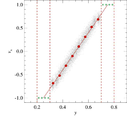
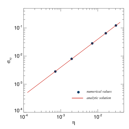
Figure 1: The panel on the left shows the stationary-state velocity profile of a viscous flow in between two infinite planes that move relative to each other. The small grey dots represent individual gas particles in the simulation (only every 25th particle has been plotted for clarity). The big red dots are mean $v_{x}$-values evaluated in equally sized $y$-bins. The green diamond symbols show particles that belong to the two thin layers used to impose the boundary conditions, while the continuous solid line is the analytic solution. This run has been performed assuming a shear viscosity coefficient of $\eta\sim 0.002$ in internal code units. The mean value of the viscous stress tensor, $\sigma_{xy}$, as a function of the shear viscosity coefficient for a number of similar runs is illustrated in the right panel. In each case, the mean value of $\sigma_{xy}$ has been estimated once the flow has reached a stationary state and is plotted with a filled circle. The continuous line gives the analytic expectation.

In order to simulate this hydrodynamical problem we have set up initial conditions using a three-dimensional periodic grid with equally spaced gas particles, all of equal mass and pressure, and being initially at rest. The aspect ratio of the box was shorter in the $y$-direction. The motion of the two planes was imposed by treating the particles in two thin sheets adjacent to the planes as ’boundary particles’, giving them the velocity of the corresponding plane, and preventing them from feeling hydrodynamical forces, i.e. they always keep moving with their initial velocity.

When the simulation is started, the $x$-component of the gas velocity develops a linear dependence on $y$ under the action of the shear viscosity, and soon the flow becomes stationary. The time needed to reach the stationarity depends on the amount of shear viscosity. The more viscous the medium, the sooner the flow reaches the steady state. Note that the same behaviour cannot be obtained with the standard artificial viscosity. Also, the presence of some amount of artificial viscosity besides the given shear viscosity perturbs the linear dependence of the velocity on the $y$-coordinate.

In the left panel of Fig. 1, we show the $x$-component of the gas velocity as a function of $y$ when the flow has reached stationarity. The grey little dots represent individual gas particles, while the red big dots denote the mean $v_{x}$ evaluated in equally sized $y$-bins. The solid line is the analytic solution, while the diamonds denote particles that are part of the boundary layers of the finite dimension of $0.1$, one moving with a velocity $v_{x}=-1$, the other with $v_{x}=1$. It can be seen that the numerical result is reproducing the analytic solution with good accuracy. Note that the gas velocity near the planes cannot reach the theoretically expected value, because it is here fixed to the value prescribed for the two boundary layers. A finite width of these layers is necessary to impose the boundary conditions in a numerically robust way, but by using a larger particle number, the thickness of this region could be made arbitrarily small, if desired. In the right panel of Fig. 1, we show the mean value of the $xy$-component of the viscous stress tensor as a function of the shear viscosity coefficient adopted in a specific run. The numerical values for the stress tensor have been evaluated once the flow has reached a stationary state. The filled circles give the mean value of $\sigma_{xy}$ for the different runs, while the solid line is the analytic fit. It can be seen that the analytic solution is recovered with high accuracy for a significant range of shear viscosities.

4.2 Flow between two planes with a constant gravitational acceleration

Another elementary hydrodynamic problem involves the viscous flow of a fluid between two planes under the action of a constant gravitational acceleration. This problem is equivalent to the classic example of a flow with a constant pressure gradient (Landau & Lifshitz, 1987). The initial situation is quite similar to the previous problem, but this time the planes do not move with respect to each other. However, there is a constant gravitational acceleration acting along the $x$-axis. Again, we consider an incompressible fluid, so that for symmetry reasons all quantities depend only on $y$ if a stationary laminar flow develops. The velocity is expected to exhibit a characteristic quadratic dependence on $y$, of the form

$$v_{x}(y)=-\frac{\rho}{2\eta}\frac{{\rm d}\Phi}{{\rm d}x}y^{2}+c_{1}y+c_{2}\,,$$ (34)

where $\rho$ is the gas density, $\Phi$ is the gravitational potential, and $c_{1}$ and $c_{2}$ are two constants defined by the boundary conditions. Again, the only non-trivial component of the viscous shear tensor is $\sigma_{xy}$, and it is related to the velocity field in the same way as in equation (33).

The initial conditions for a numerical model of this problem were set up as before, except that a constant gravitational acceleration along the $x$-axis was imposed. All particles were initially at rest, and the particles of the two boundary layers were made to ignore the gravitational field so that their positions stayed fixed. In Fig. 2, we show a measurement of the velocity of the gas particles once the flow reached a stationary state. The grey little dots are individual particles in the simulated region between the planes, while the green diamond symbols represent particles of the boundary layers. The solid line gives the analytic solution, while the big red dot shows the average velocity of gas particles for $y=0.5$. The central part of the flow matches the characteristic quadratic form of the analytic solution accurately, with a maximum gas velocity corresponding closely to the analytic solution, even though the simulated gas velocity near the planes is a bit lower than the analytic expectation. Again, the latter effect is to be expected due to the finite width of the boundary layers, which also influences the properties of the flow in their immediate vicinity.

We note that the magnitude of the velocity scatter of individual particles around the mean profile depends on the strength of the adopted gas pressure relative to the viscous forces. Even for parameter choices where this scatter becomes large, the mean velocity field tracks the analytic solution well in all cases we examined, indicating that our implemented scheme is quite robust.

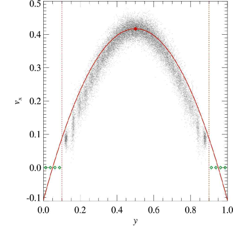
Figure 2: Velocity profile for the viscous flow between two fixed planes in a field of constant gravitational acceleration. The little grey dots are the individual particles from the simulation output (only every 25th particle has been plotted for clarity). The analytic solution with its characteristic quadratic velocity dependence on the $y$ coordinate is shown with a red solid line. The big red dot marks the mean velocity of gas particles for $y=0.5$, while the green diamond symbols represent the particles that belong to the layers of particles used to impose the boundary conditions.

4.3 Shock tube tests

In this section, we examine whether our new implementation of physical viscosity can also be used to capture shocks, and how this fares with respect to results obtained with the standard artificial viscosity. For this purpose, we performed a number of shock tube simulations which have been setup following the standard approach outlined in Sod (1978). We considered both mild shocks with a Mach number of order 1.5, and also stronger shocks up to a Mach number of 10. These tests allow us to constrain the amount of physical shear and/or bulk viscosity needed to capture the shocks accurately, and hence to assess if and how much artificial viscosity is still required in simulations of viscous gases.

Our initial conditions consist of a three-dimensional periodic box that is elongated in the $x$-direction, with a total length $L$. The box is filled with gas particles of equal mass arranged on a grid. The left half of the box ($x<L/2$) has a higher initial pressure with respect to the right half ($x>L/2$), such that shocks of different strength can be driven into the right side, depending on the initial pressure ratio. The adopted adiabatic index is $\gamma=1.4$. All gas particles are initially at rest, and we have evolved the simulations until a final time of $t=3.5$.

Before we discuss the results it should be noted that there is an important conceptual difference between simulations with our new implementation of internal friction and simulations that use the artificial SPH viscosity. In the former case we consider real gases which have different hydrodynamical properties in the region of shocks (where the velocity field has strong gradients) than ideal fluids for which the analytic solutions of shock tubes refer to. In order to properly treat real fluids in shocks, one in principle needs to invoke the kinetic theory of gases, because the mean free path of particles is of the order of the shock width. This is beyond the scope of this work. However, the analytic solutions for ideal gases outside the shock region provide a very good approximation because the viscous forces there are negligible, as we will explicitly confirm below.

In Fig. 3, we show the profile of gas density, velocity, entropy and pressure in a shock tube calculation where the gas particles experience a shock of strength ${\cal M}=1.48$. The simulation results are represented by blue circles, the dotted lines denote the initial conditions, and the continuous red lines give the analytic solution, obtained by solving the hydrodynamical equations of an ideal gas with imposed Rankine-Hugoniot conditions (e.g. Courant & Friedrichs, 1976; Rasio & Shapiro, 1991). The three different columns give results for the standard artificial viscosity with $\alpha=0.7$ (left panel), physical shear viscosity with $\eta=0.04$ (middle panel), and physical bulk viscosity of $\zeta=0.03$ (right panel). The only difference between these three runs lies in the gas viscosity, all the other code parameters and the initial conditions were kept exactly identical in order to facilitate a clear comparison. Fig. 3 shows that the numerical model for physical viscosity is capable of capturing the shock, and it results in quite accurate estimates of the post-shock quantities. This holds both for shear and bulk viscosity. Compared to the case with an artificial viscosity, there is more velocity noise in the postshock region, however. Also, the shock front itself is sharper when an artificial viscosity is used, and the analytic solution for the rarefaction wave is recovered more accurately in the transition region to the constant density sections of the flow. In general, the physical viscosity solutions appear more smoothed in the transition regions between the different parts of the flow.

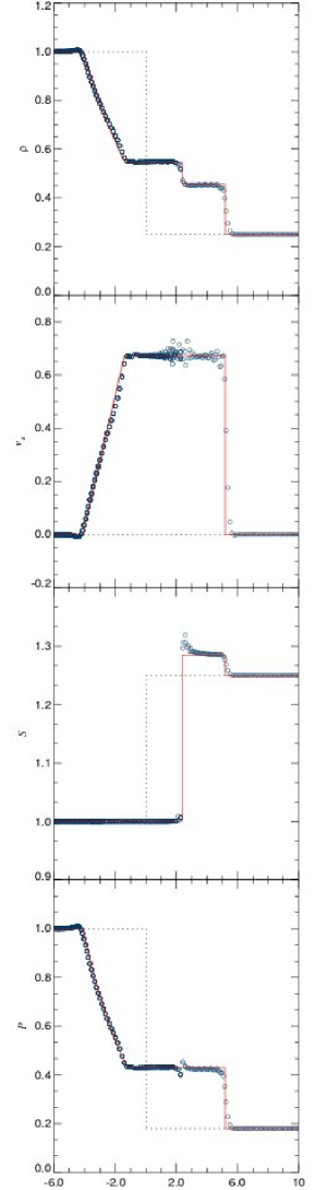
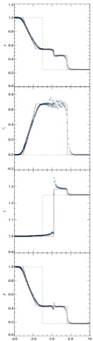
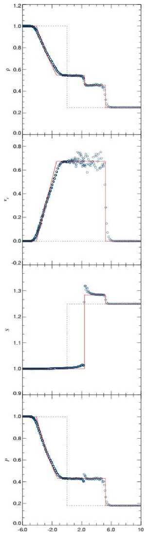
Figure 3: Hydrodynamical properties along a shock tube simulation with a shock of Mach number ${\cal M}=1.48$, at time $t=3.5$. The initial conditions are drawn with doted lines, the analytic solutions are shown with continuous red lines, and the symbols give the SPH result. The three vertical columns refer to a run carried out with the standard artificial viscosity (left column), to one with physical shear viscosity instead (middle column), or to one with physical bulk viscosity (right column). From top to bottom, the individual rows show the profiles of density, velocity, entropy, and pressure, respectively.

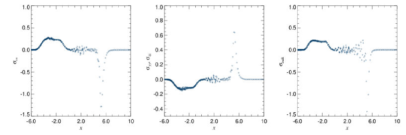
Figure 4: Viscous stress tensor profile in the case of a ${\cal M}=1.48$ shock tube simulation. The first two panels refer to the physical shear viscosity, showing diagonal components of the stress tensor, while in the right panel the bulk stress tensor is plotted. In the middle panel, the dots give only results for $\sigma_{yy}$, because the $\sigma_{yy}$ and $\sigma_{zz}$ components of the shear tensor show a practically identical dependence on the $x$-coordinate, given the symmetry of the problem.

In Fig. 4, we examine the viscous stress tensor of gas particles in this problem. The first two panels show the diagonal components of the shear stress tensor, while the last panel gives the bulk viscosity tensor. The viscous stress tensor is different from zero only in the region between the head of the rarefaction wave and the shock wave, implying that the viscous forces are important in that region and are negligible elsewhere. The $\sigma_{yy}$ and $\sigma_{zz}$ components of the shear tensor behave almost identically because of the symmetry of the problem, and thus in the middle panel of Fig. 4 the dots are for $\sigma_{yy}$ only. It can be noted that $\sigma_{xx}$, $\sigma_{yy}$ and $\sigma_{zz}$ have sign and magnitude such that their sum is zero to high accuracy, as it should be given that the shear tensor is traceless. Also, the off-diagonal components of the shear stress tensor are negligible, as expected. The bulk stress tensor shows very similar features as the $\sigma_{xx}$ component of the shear tensor, due to the fact that the dominant term in both cases is $\partial v_{x}/\partial x$. However, $\sigma_{\rm bulk}$ shows more scatter for $x\in[3,5]$ because the noise in the remaining velocity derivatives in the corresponding simulation is larger. In our simulations with with larger Mach numbers, we obtained qualitatively very similar results as the ones presented in Fig. 4.

The above analysis has shown that both shear and bulk physical viscosity are in principle capable of capturing shocks, provided the viscosity coefficients are sufficiently large. This means that in simulations of low Reynolds number one can probably avoid the use of any additional artificial viscosity. In general however, it seems clear that an artificial viscosity is still needed even when physical viscosity is modelled. This is simply because the strength of the physical viscosity can be quite low, and can vary locally with the flow if a physical parameterization like that of Braginskii is used. Without artificial viscosity, shocks would then not be captured accurately in a narrow shock front, and particle interpenetration would not be properly avoided. Instead, strong fluid instabilities could develop in the shock region, growing to such large enough size that the residual physical viscosity can damp them out. In the rest of our study, we will therefore invoke when necessary an additional artificial viscosity in the standard way when we model physical viscosity in astrophysically interesting situations. This guarantees that shocks are always captured equally well as in standard SPH.

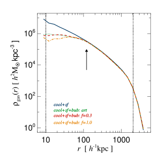
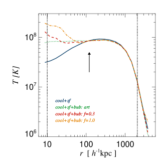
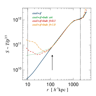
Figure 5: Radial gas profiles of a $10^{15}\,h^{-1}{\rm M_{\odot}}$ isolated halo at time $t=0.15\,t_{\rm Hubble}$. We show the gas density (left panel), mass-weighted temperature (middle panel), and gas entropy (right panel), and compare runs with cooling and star formation only (blue solid lines) with runs having additional AGN heating as well. The green dotted lines are for simulations with standard artificial viscosity. The red dashed lines give results when the Braginskii parameterization of the shear viscosity is “switched on”, with a suppression factor of $0.3$. For comparison, the orange dot-dashed lines show the results when no suppression factor is used for the shear viscosity.

5 AGN–driven bubbles in a viscous intracluster medium

In this section, we study the interaction of AGN-induced bubbles with a viscous intracluster medium. This represents an extension of the study of Sijacki & Springel (2006), and we refer to this paper for a detailed description of the models, and the simulation setup, while we here give just a brief overview.

We consider models of isolated galaxy clusters under a range of different physical processes. The initial setup consists of a static NFW dark mater halo (Navarro et al., 1996, 1997), and a gas component which is initially in hydrostatic equilibrium. The adopted initial gas density profile closely follows the dark mater profile, except for a slightly softened core. A certain level of rotation has been included as well, described by a spin parameter of $\lambda=0.05$. AGN heating has been simulated with a phenomenological approach in the form of centrally concentrated hot bubbles that are injected into the ICM in regular time intervals. The basic parameters of the AGN feedback scenario are the bubble radius, distance from the cluster centre, duty cycle and bubble energy content. These parameters have been constrained by recent cluster observations and also by the basic empirical laws of black hole accretion physics.

We used $10^{6}$ gas particles to construct initial conditions for a massive isolated galaxy cluster of mass $10^{15}\,h^{-1}{\rm M_{\odot}}$, with a spatial resolution in the gravitational field equal to $6.5\,h^{-1}{\rm kpc}$. Starting from these identical initial conditions, we carried out different runs, characterized as follows: (1) radiative cooling and star formation together with standard artificial viscosity; (2) cooling, star formation, and AGN-bubble heating with artificial viscosity; (3) cooling, star formation, AGN-bubble heating, and physical shear viscosity, based on the Braginskii parameterization and with a suppression factor that we varied in the range of $0.3$ to $1.0$. The radius of the bubbles was chosen as $30\,h^{-1}{\rm kpc}$, and they were injected into the ICM every $10^{8}\,{\rm yrs}$ along a fixed spatial axis, with an energy content equal to $2.5\times 10^{60}\,{\rm ergs}$ per bubble.

5.1 Radial heating efficiency and profiles

In Fig. 5, we show radial profiles of our massive galaxy cluster after a simulated time of $0.15\,t_{\rm Hubble}$. Gas density is plotted in the left panel, mass-weighted temperature in the central panel, and gas entropy in the right panel. A number of interesting features can be noticed from the gas profiles. First, regardless of the assumed gas viscosity, the bubble heating prevents the creation of a strong cooling flow, and gas is heated efficiently in the inner regions. Moreover, the spatial extent of the central region in which AGN feedback alters the gas profiles does not depend on the level of gas viscosity - in all the runs, bubbles influence the ICM out to $\sim 150\,h^{-1}{\rm kpc}$. This scale is indicated with a vertical arrow on the panels. Thus, the radial extent of bubble heating is determined by other factors, like for example by the initial entropy excess of bubbles with respect to the surrounding gas, by the injection mechanism, or by the equation of state of the gas filling the bubbles. Second, it can be seen that an increase of the gas viscosity produces a systematically stronger heating in the innermost $\sim 50\,h^{-1}{\rm kpc}$, and this trend is also present at subsequent simulation output times until $0.25\,t_{\rm Hubble}$ where we stopped the simulations. The heating is most prominent in the case of unsuppressed Braginskii viscosity (orange dot-dashed lines), where an entropy inversion occurs, and the temperature of the gas keeps increasing until the very centre. Such a temperature profile is not favoured by observational findings, suggesting that if the intracluster gas viscosity is indeed so high than the bubble energy content has to be substantially lower, or the energy transport from the bubbles into the ICM has to be somehow inhibited, possibly by magnetic fields.

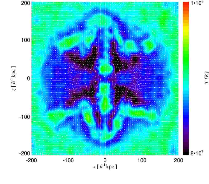
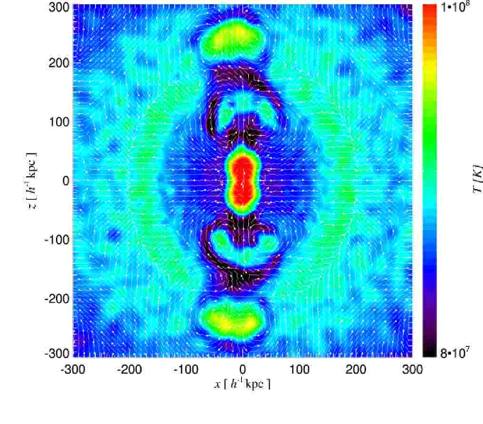
Figure 6: Mass-weighted temperature maps of a $10^{15}\,h^{-1}{\rm M_{\odot}}$ isolated halo, subject to AGN bubble feedback. The velocity field of the gas is over-plotted with white arrows. The maps show how the morphology, survival time and maximum distance reached of AGN–driven bubbles depend strongly on the amount of physical viscosity assumed: in the upper panel, the Braginskii shear viscosity has been suppressed by a factor 0.3, while in the lower panel, the simulation has been evolved with the full Branginskii viscosity.

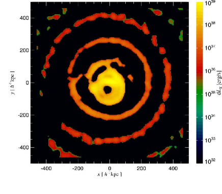
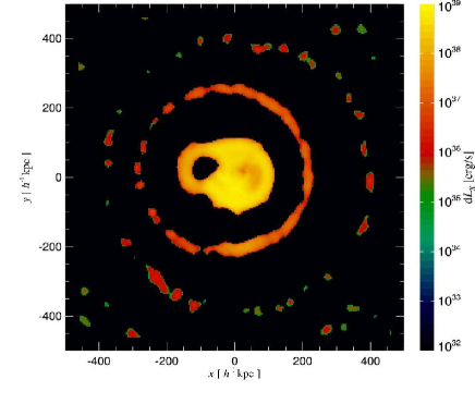
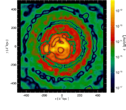
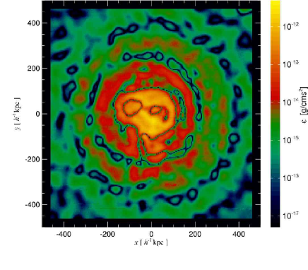
Figure 7: The upper panels show unsharp-masked X–ray emissivity maps of a $10^{15}\,h^{-1}{\rm M_{\odot}}$ isolated cluster with AGN bubble feedback. On the left, a case with lower viscosity is shown (suppression factor $f=0.3$), while on the right, a case with the maximum value of the shear viscosity is displayed (suppression factor $f=1.0$). The sound waves generated by the bubbles in the ICM are clearly more efficiently dissipated when the ICM has a higher viscosity. The panels on the bottom illustrate the projected energy density in sound waves for the same cases, estimated as explained in the text. On these maps, both compressed and rarefied regions are visible, containing a significant amount of acoustic energy density. Nevertheless, the total energy of the sound waves is not substantial in our models, and amounts to only a small fraction of the thermal energy of an injected bubble.

Another interesting feature of bubble heating in a viscous ICM can be noticed when the bubble morphologies and the radial heating efficiency are examined in more detail. In Fig. 6, we show mass-weighted temperature maps of the central cluster regions, for the case of Braginskii viscosity with suppression factor of $0.3$ (upper panel) and for unsuppressed Braginskii shear viscosity (lower panel). The velocity flow pattern is indicated with white arrows on these maps. Even though the radial extent of the bubble heating is similar for different magnitudes of internal friction, the morphologies of evolved bubbles, their maximum clustercentric distance reached and their survival times vary. When the gas viscosity is as high as the full Braginskii value, the bubbles rise up to $\sim 300\,h^{-1}{\rm kpc}$ in the cluster atmosphere without being disrupted, and traces of two up to three past bubble episodes can be detected, indicating that the bubbles survive at least as long as $\sim 2\times 10^{8}\,{\rm yrs}$. However, when the gas viscosity is lowered (upper panel of Fig. 6) bubbles typically start to disintegrate at $\sim 150\,h^{-1}{\rm kpc}$ and multiple bubble events can typically not be identified.

This suggests that a relatively high amount of gas viscosity may be needed to explain the recent observations of the Perseus cluster (e.g. Fabian et al., 2006), where several bubble occurrences have been detected. However, an alternative explanation could be that the bubbles are stabilized against fluid instabilities by magnetic fields at their interface with the ICM instead of by viscosity. A relativistic particle component (cosmic rays) filling the bubble will also change the dynamical picture. Nevertheless, it is interesting that the observed morphology of bubbles can in principle constrain the level of ICM viscosity, an aspect that we plan to explore further in a future study.

In the velocity fields shown in Fig. 6, it can be seen that the flow of the gas in the wake of the bubbles is approximately laminar, while at the bubble edges the velocity field shows a significant curl component. This perturbed motion is not only present for the most recently injected bubbles, but also for the bubbles that are already $\sim 2\times 10^{8}\,{\rm yrs}$ old, albeit with a smaller magnitude. In the case of the full Braginskii viscosity the magnitude of the velocity perturbations induced by the bubbles is of the order of $\lower 3.22916pt\hbox{$\sim$}\hbox to0.0pt{\hss\raise 1.1625pt\hbox{$<$}}\,100\,{\rm km\,s^{-1}}$ for the recent bubbles, while it decreases to $\lower 3.22916pt\hbox{$\sim$}\hbox to0.0pt{\hss\raise 1.1625pt\hbox{$<$}}\,20\,{\rm km\,s^{-1}}$ for the older ones.

5.2 Sound waves dissipation

We also examined how the occurrence of sound waves produced by the bubbles and the associated non-local heating is influenced by different amounts of ICM viscosity. In Fig. 7, we show unsharp-masked images of the X–ray emissivity, produced by subtracting a map smoothed on a $50\,h^{-1}{\rm kpc}$ scale from the original luminosity map. It is clear that for higher gas viscosity (right panel, unsuppressed Braginskii value) the damping of sound waves in the central region is stronger than for a simulation with lower viscosity (left panel: $0.3$ of Braginskii viscosity). Nevertheless, the radial profiles of the gas entropy show that only in the inner $\sim 50\,h^{-1}{\rm kpc}$ a more efficient heating of the ICM can be observed when the viscosity is increased. This suggests that the energy content of the sound waves produced by the bubbles is not very large and probably not capable of providing significant heating at larger radii.

Simulation	$N_{\rm HR}$	$N_{\rm gas}$	$m_{\rm DM}$ [$\,h^{-1}{\rm M}_{\odot}\,$]	$m_{\rm gas}$ [$\,h^{-1}{\rm M}_{\odot}\,$]	$z_{\rm ini}$	$z_{\rm fin}$	$\epsilon$ [$\,h^{-1}{\rm kpc}\,$]
g1/g8	$4937886$	$4937886$	$1.13\times 10^{9}$	$0.17\times 10^{9}$	$60$	$0$	$5.0$

Table 1: Numerical parameters of the cosmological galaxy cluster simulations used in this study. The values listed from the second to the fifth column refer to the number and to the mass of high resolution dark matter particles and of gas particles. Note that the actual values of $N_{\rm gas}$ and $m_{\rm gas}$ may vary in time due to star formation, if present. The last three columns give the initial and final redshifts of the runs, and the gravitational softening length $\epsilon$.

In order to put more stringent constraints on the influence of the sound waves, we have estimated their energy content by evaluating (Landau & Lifshitz, 1987)

$$\int E_{s}\,{\rm d}V\,=\,\int\rho_{0}v^{2}\,{\rm d}V\,=\,\int\frac{{\rho^{\prime}}^{2}}{\rho_{0}}c_{s}^{2}\,{\rm d}V,$$ (35)

where $E_{s}$ is the sound energy density, $\rho_{0}$ is the unperturbed gas density, $v$ is the fluid velocity, $\rho^{\prime}$ is the change in gas density due to the sound waves, and $c_{s}$ is the sound speed. Strictly speaking, this equation is valid only for travelling plane waves, but it should still provide us with a reliable order of magnitude estimate of the sound waves energy in our geometrically more complex case. We computed projected energy density maps (see lower panels of Fig. 7) by taking the smoothed density field for $\rho_{0}$, while we estimated $\rho^{\prime}$ as the difference between the actual density field and the smoothed one. Both compressed regions (which correspond to the rings in the upper panels) and rarefied regions store a considerable amount of energy. However, it should be noted that the sound wave energy in the rarefaction regions is overestimated when computed in this way, because the bubbles themselves contribute to it, being underdense with respect to the background and having similar dimension to the smoothing scale. Nevertheless, when the total sound wave energy is estimated in this way we obtain $\sim 5\times 10^{59}\,{\rm ergs}$, which is only a small fraction of the initially injected bubble energy. As pointed out by Churazov et al. (2002), a number of the same order of magnitude is obtained if as a crude estimate of the sound wave energy one considers the sound waves generated by the motion of a solid sphere through a medium of a given density $\rho$ (Landau & Lifshitz, 1987).

Based on these findings, the viscous damping of sound waves provides only an insignificant contribution in coupling the AGN-injected energy into the ICM. Note that in these models of isolated halos we have deliberately included physical shear viscosity only. Thus, our estimate for the damping of sound waves is not affected by any residual artificial viscosity. A caveat, however, is that our simulations do not self-consistently model the initial phase of bubble injection, where the AGN-jet deposits its energy and inflates the bubble. It is conceivable that the associated processes produce energetically more important sound waves and weak shocks, which could then increase the importance of viscous damping of sound waves compared to the result found here.

6 Cosmological simulations of viscous galaxy clusters

In this section we discuss the effects of internal friction on clusters of galaxies formed in fully self-consistent cosmological simulations. We have carried out a variety of runs that follow different physical processes, including non–radiative hydrodynamical simulations, described in detail in Section 6.1, and runs with radiative gas cooling, star formation and feedback processes, which are discussed in Section 6.2. For all these simulations, we carried out matching pairs of runs without physical viscosity and with physical shear viscosity (using the Braginskii parameterization with a suppression factor of 0.3), in order to be able to clearly identify differences due to the viscous dissipation processes.

For our simulations, we selected two massive galaxy clusters that have been extracted from a cosmological $\Lambda$CDM model with a boxsize of $479h^{-1}{\rm Mpc}$ (Yoshida et al., 2001; Jenkins et al., 2001), and were prepared by Dolag (2004) for resimulation at higher resolution using the Zoomed Initial Condition technique (Tormen et al., 1997). In Tables 1 and 2, we summarize the basic parameters of the simulations and the main physical properties of the galaxy clusters. The cosmological parameters of the simulations correspond to a concordance $\Lambda$CDM model with $\Omega_{m}=0.3$, $\Omega_{b}=0.04$, $\sigma_{8}=0.9$, and $H_{0}=70\,{\rm km\,s}^{-1}{\rm Mpc}^{-1}$ at the present epoch.

Cluster	$R_{\rm 200}$	$M_{\rm 200}$	$T_{\rm mw}$	$L_{\rm X}$
	[$\,h^{-1}{\rm kpc}\,$]	[$\,h^{-1}{\rm M}_{\odot}\,$]	[K]	[$\,\rm ergs^{-1}\,$]
g1_csf	$2857$	$1.63\times 10^{15}$	$7.3\times 10^{7}$	$1.0\times 10^{45}$
g1_csfv	$2832$	$1.58\times 10^{15}$	$8.1\times 10^{7}$	$1.0\times 10^{45}$
g8_ad	$3306$	$2.52\times 10^{15}$	$9.7\times 10^{7}$	$1.1\times 10^{46}$
g8_adv	$3276$	$2.45\times 10^{15}$	$1.1\times 10^{8}$	$4.5\times 10^{45}$

Table 2: Physical properties of our sample of simulated galaxy clusters at $z=0$ and at $200\rho_{c}$. For two different galaxy clusters, labelled in the first column, and for the different runs, cluster radius, total mass, mass–weighted gas temperature and X–ray luminosity are listed, respectively. Subscripts in the first column denote runs including different physics, namely cooling and star formation for the g1 cluster, and non–radiative gas hydrodynamics for the g8 cluster, in both cases also with Braginskii shear viscosity with suppression factor of 0.3.

6.1 Non–radiative simulations

In Fig. 8, we show projected gas density maps at different redshifts for our non-radiative cluster simulations. It is evident that already at early times, at around $z\sim 5$, the gas distribution in the presence of shear viscosity (panels on the right) starts to deviate substantially from the corresponding simulation without internal friction (panels on the left). Also, the amount of gas that is bound to dark matter subhalos is reduced, and there appears to be more diffuse gas in the outskirts of massive objects. Furthermore, small structures that are falling into the most massive halo at each epoch (located in the centre of the panels), lose their gas content more quickly due to the shear forces, and feature prominent tails that extend up to several hundred kiloparsec. These general features are present at all epochs from $z\sim 5$ to $z=0$. At low redshifts, however, the central parts of the main halo appear quite similar, although the central density is somewhat reduced in the simulation with physical viscosity, while there appears to be more diffuse gas with a smaller number of prominent gas concentrations in the outskirts. These trends can be readily understood as a consequence of viscous dissipation, which increases the stripping of gas and helps to expel gas from shallow dark matter potential wells in the infall regions of larger structures.

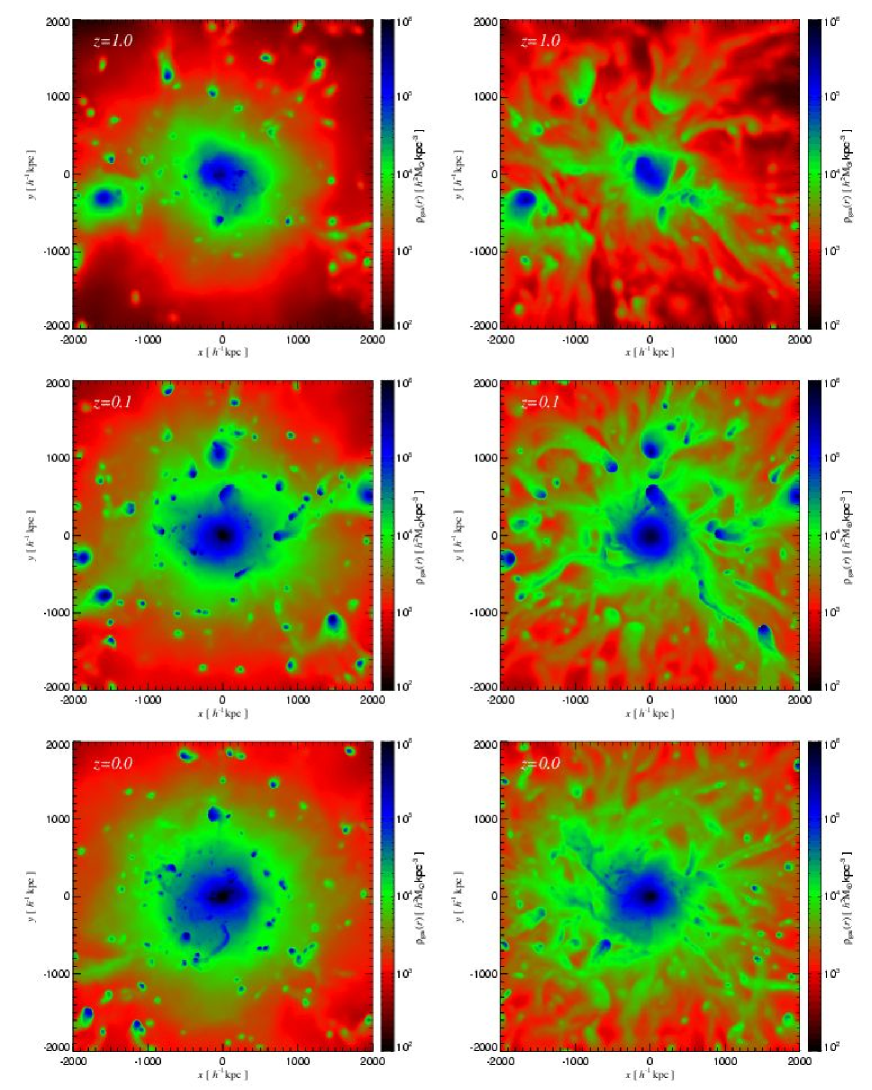
Figure 8: Projected gas density maps of the g8 galaxy cluster simulation at redshifts $z=1.0$, $z=0.1$ and $z=0.0$, as indicated in the upper-left corner of the panels. The panels in the left column show the gas density distribution in the case of a non–radiative run, while the panels in the right column give the gas density distribution when Braginskii shear viscosity is “switched-on”, using a suppression factor of 0.3. It is evident from these panels that the presence of a modest amount of shear viscosity has a significant impact on the gas distribution, removing more gas from infalling structures when they enter the massive halo, and producing pronounced gaseous tails behind them.

A more quantitative analysis of how viscosity affects the thermodynamics of clusters is obtained by studying the radial profiles of gas density, mass-weighed temperature, and entropy. In Fig. 9, we compare these profiles at two different epochs, $z=1$ and $z=0$. The solid blue line refers to the non-radiative run, while the dotted green line gives the result when physical shear viscosity is included. The effects of viscosity increase systematically with time, and manifest themselves in a reduction of the gas density throughout the cluster. The suppression is particularly strong in the very centre, where it reaches almost an order of magnitude at $z=0$. At early times, the temperature is mainly boosted in the outer regions of the cluster, while for $z<0.5$, also the central gas temperature starts to be significantly increased. As a consequence, the entropy profile shows two different features: At early times, the central rise of entropy is caused by a lower gas density, while at late times, the entropy is even more enhanced in the inner regions, out to a radius of $\sim 100\,h^{-1}{\rm kpc}$, because of a lower gas density and an increased temperature. In the outer parts of the halo, the increase of the gas entropy is always a result of the joint action of temperature and density change. We will come back to a discussion of the physical reason for this behaviour in Section 6.2.

As a consequence of the strong modification of the density and temperature structure of the cluster in the viscous case, we also find a significant reduction of the X–ray luminosity. This is reflected in Table 2, which lists some of the basic properties of these clusters. Interestingly, a similar change of the X–ray luminosity is not found in the case of the simulations that also include cooling and star formation, which we will discuss next.

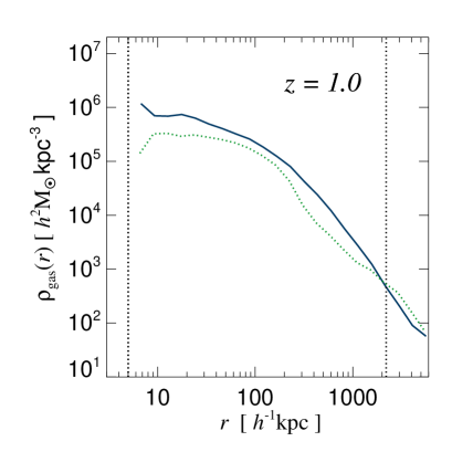
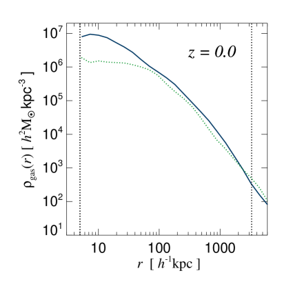
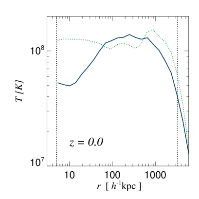
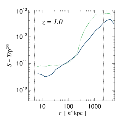
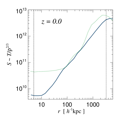
Figure 9: Radial profiles of gas density, mass-weighted temperature, and entropy of the ‘g8’ galaxy cluster simulation. The blue continuous lines are for the non–radiative run, while the dotted green lines are for the run with additional Braginskii shear viscosity with suppression factor of 0.3. The panels in the left column refer to the gas profiles evaluated at $z=1.0$, while the ones in the right column are for $z=0$. The dotted vertical lines denote the gravitational softening length and the virial radius at the given redshift.

6.2 Simulations with cooling and star formation

In Fig. 10, we show the radial gas profiles of basic thermodynamic quantities of our cluster simulations that included radiative cooling and star formation, either without (blue solid line) or with (dotted green line) additional shear viscosity. At high redshifts, the signatures of viscosity are quite similar to the previously considered case where gas cooling was absent. However, the formation of a cooling flow for $z<0.5$ changes the central gas properties dramatically at later times. Even though viscous dissipation is acting in the cluster centre, the gas cooling times become so short there that all the thermal energy gained from internal friction is radiated away promptly. In fact, the gas starts to cool even more in the central regions in the viscous case, as can been seen from the entropy profiles at $z=0$. The gas density is increased in the innermost regions as well.

Apparently, while the viscous heating in the centre is not sufficiently strong to raise the temperature significantly, the mild heating does reduce the star formation rate and therefore the associated non-gravitational heating from supernovae. The net result is an increase in the X–ray luminosity due to the sensitive density- and temperature-dependence of the cooling luminosity. Interestingly, there is still a reduction of the X-ray luminosity in the outskirts of the cluster in the viscous simulation, because the gas density is lowered there, but this is just compensated for by a matching increase in the inner parts. Another important aspect of the viscous heating process is that it makes the temperature profile closer to isothermal, suggesting that the viscosity helps to level the temperature of the cluster on large scales. It is interesting to note that our results on the profiles resemble the findings of self-consistent cosmological simulations of cluster formation with thermal conduction (Jubelgas et al., 2004; Dolag et al., 2004). The transport coefficients of viscosity and heat conductivity have the same temperature dependence, and this fact may contribute to the similarity of the behaviour with respect to the role these transport processes play in shaping the gas properties.

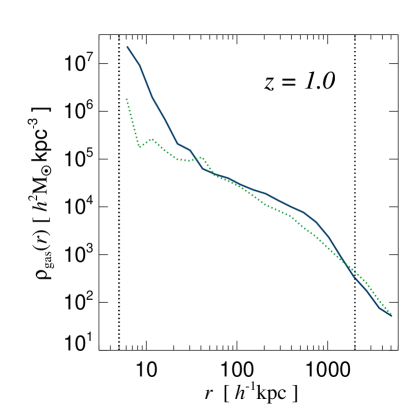
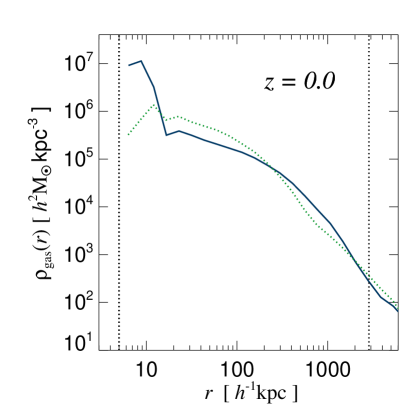
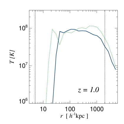
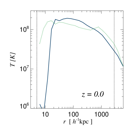
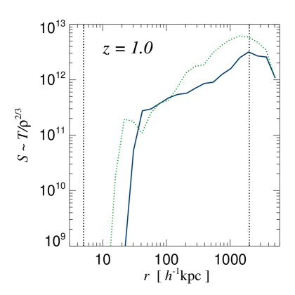
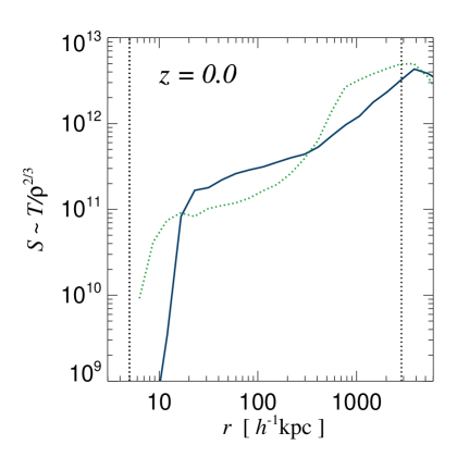
Figure 10: Radial profiles of gas density, mass-weighted temperature, and entropy of the ‘g1’ galaxy cluster simulation. The blue continuous lines are for the run with cooling and star formation, while the dotted green lines are for the run with additional Braginskii shear viscosity with suppression factor of 0.3. The panels in the left column refer to the gas profiles evaluated at $z=1.0$, while the panels in the right column are for $z=0$. The dotted vertical lines indicate the gravitational softening length and the virial radius at the given redshift. It can been seen that the viscous effects are similar to the non–radiative case at high redshifts, while they differ significantly at low $z$ due to the formation of a central cooling flow.

We now turn to a discussion of the radial dependence of viscous dissipation in clusters of galaxies. As can be seen from equation (25), the entropy increase due to shear viscosity involves two factors: one is given by the shear viscosity coefficient, which basically has only a dependence on temperature to the $5/2$ power, and the other is the ratio of the rate-of-strain tensor squared to that of the gas density elevated to the $\gamma$. Thus, viscous entropy injection will be favoured in regions of high temperature, low density and strong velocity gradients. In order to disentangle the relative importance of these different dependencies we show the radial profiles of the shear viscosity coefficient $\eta$, the rate-of-strain tensor squared $\sigma_{\alpha\beta}^{2}$, and of the kinematic viscosity $\nu$ in Fig. 11, at $z=0$.

Let us first consider the non–radiative case, which is shown with solid green lines. At all radii, the gas density is reduced in the presence of shear viscosity, and this modification of the density profile influences the rate of entropy production. Nevertheless, the contribution of the shear coefficient is more important in the outer regions, for $r>100\,h^{-1}{\rm kpc}$, having a maximum at $\sim 1000\,h^{-1}{\rm kpc}$, where also the gas temperature is highest. On the other hand, the rate-of-strain tensor is monotonically increasing from the outskirts towards the centre, and this is also true for its individual components, indicating that the velocity gradients are largest in the inner regions.

The dashed red lines show the results when cooling and star formation are included. The differences that arise in the shear viscosity coefficient compared with the non-radiative case can be simply explained by the different temperature profiles: in the outer regions, for $r>100\,h^{-1}{\rm kpc}$, the ‘g1’ cluster run has lower $\eta$ because its temperature there is smaller due to the fact that this cluster is somewhat less massive than the ‘g8’ galaxy cluster. Instead, the temperature of the ‘g1’ cluster in the innermost regions is larger, because the introduction of radiative cooling increases the central gas temperature, except for the innermost cooling flow region. Also, $\sigma_{\alpha\beta}^{2}$ of the ‘g1’ cluster is higher near the centre due to the motions induced by the prominent cooling flow that has formed in it.

Finally, we study the kinematic viscosity in the last panel of Fig. 11, which is given by the ratio of the shear viscosity coefficient to the gas density. Both for the ‘g1’ and ‘g8’ cluster simulations, the kinematic viscosity coefficient is very similar in the outer regions, and is highest for large radii. In the inner $100\,h^{-1}{\rm kpc}$, the kinematic viscosity of the ‘g1’ cluster is higher, due to the efficient gas cooling. Overplotted with a blue arrow is an upper limit for the kinematic viscosity on a scale of $100\,{\rm kpc}$ estimated for the Coma galaxy cluster by Schuecker et al. (2004). The kinematic viscosity of the ‘g8’ galaxy cluster, which is slightly more massive then the Coma cluster, is in agreement with this observational constraint, suggesting that a suppression factor as large as 0.3 is not ruled out observationally. On the other hand, the kinematic viscosity of the ‘g1’ cluster, with the same suppression factor, is only marginally in agreement with the observational upper limit. However, this comparison needs to be taken with a grain of salt: The intrinsic amount of shear viscosity is certainly overestimated in our simulations, because they suffer from strong central cooling flows which are not observed in real galaxy clusters.

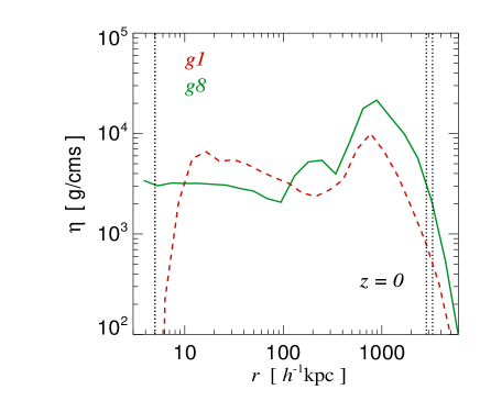
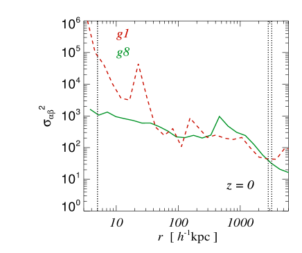
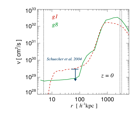
Figure 11: From top to bottom, radial profiles of the mass-weighted shear viscosity coefficient, of the rate-of-strain tensor squared, and of the kinematic viscosity coefficient in the ‘g1’ and ‘g8’ galaxy cluster simulations, respectively. The red dashed line is for the g1 simulation with cooling, star formation and shear viscosity, while the continuous green line represents the non-radiative g8 simulation with the same amount of shear viscosity. The dotted vertical lines indicate the gravitational softening and the virial radius at $z=0$, respectively. In the bottom panel, the observational upper limit for the Coma galaxy cluster (Schuecker et al., 2004) at a scale of $100\,{\rm kpc}$ is shown with a blue arrow.

6.3 Viscous dissipation during merger events

The radial profiles of gas temperature and entropy discussed above indicate that the gas is heated very efficiently in cluster outskirts by viscous dissipation during accretion and merger events. In this section, we study this phenomenon in more detail. In particular, we analyze the spatial distribution of entropy production just before and during a merger episode. To this end we compare projected density maps, which give us an indication on the exact position and extent of the merging clumps, to entropy maps, which tell us where the heating takes place. In Fig. 12, we show an example of these maps for the ‘g1’ galaxy cluster. The upper panels refer to the run with cooling and star formation only, and the lower panels show the run where shear viscosity was included as well. The panels for the runs with different physics are not at the same redshift because the shear forces influence the dynamics of structure formation sufficiently strongly that timing offsets in the merging histories occur. We tried however to select snapshots with similar merging configuration at comparable cosmic epochs so that the visible differences arise primarily because of the introduction of the shear viscosity. We note that we analyzed a number of different merger configurations at multiple redshifts, also considering the non–radiative simulations. We find that the features visible in Fig. 12 are ubiquitous; viscous dissipation of shear motions not only considerably boosts the gas entropy, but also generates this entropy in special spatial regions which have no counterparts in the simulations that only include an artificial viscosity. The relevant regions are located perpendicular to the direction of a halo encounter, and appear as entropy-bright bridges. These regions of enhanced entropy, which are never found in the runs without shear viscosity, are responsible for heating the clusters outskirts, already at early times.

We have also constructed maps of the viscous entropy increase, based on equation (25). All the filamentary high entropy regions are corresponding to the ones shown in Fig. 12, demonstrating that they are caused by $\eta\,\sigma_{\alpha\beta}^{2}/\rho^{\gamma}$. The dominant factor appears to be $\eta/\rho^{\gamma}$, while the spatial distribution of $\sigma_{\alpha\beta}^{2}$ is preferentially confined to the regions characterized by relatively high overdensities.

Finally, in order to better understand the gas dynamics in these high entropy regions, we computed the velocity flow field during the merger event, and show it overlaid on the X–ray emissivity map in Fig. 13. It can be seen that there are two galaxy clusters approaching each other, one located in the centre of the figure and the other one being above it, at $(x,y)\sim(0,1000)\,h^{-1}{\rm kpc}$. The high entropy bridge is lying between the merging clusters, roughly perpendicular to their direction of motion. Considering the velocity flow pattern, it can be noticed that there are two velocity streams: one starting from the lower right corner, and the other from the upper right one. The velocity currents meet in the central region where the merger will occur. Therefore, the gas is not flowing along the high entropy bridge, but rather perpendicular to it. This shows that the material of the high entropy bridge is not funneled towards the centre from the cluster outskirts but rather that it is heated in situ by significant viscous dissipation, creating the entropy bridges between the merging structures.

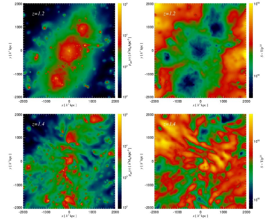
Figure 12: Projected maps of gas density and entropy for the g1 galaxy cluster simulation, at an instant just before a merger event. The upper panels are for the run with cooling and star formation, while the lower panels, at somewhat different redshift, are for the run with additional shear viscosity. It can be seen that the entropy of the gas is considerably boosted by internal friction processes (note the different scales of the entropy maps), and in addition it appears that much of this entropy is generated in different regions which have a filamentary kind of structure.

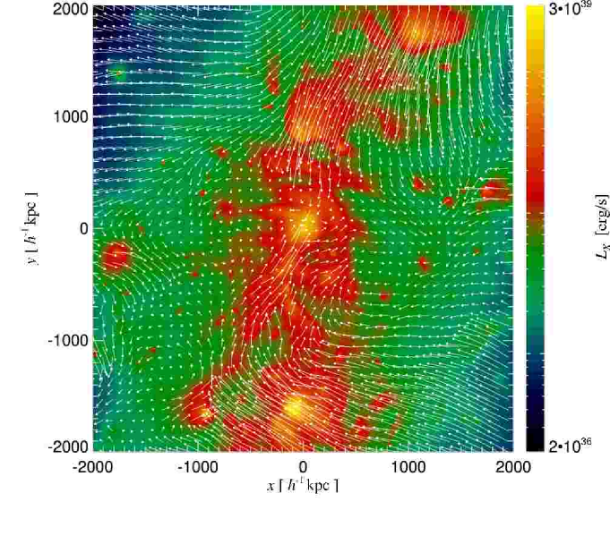
Figure 13: Projected X–ray emissivity map of the g1 galaxy cluster, simulated with physical viscosity. The map corresponds to the lower panel of Fig. 12, but here the velocity field is overplotted with white arrows. The flow field suggests that the bright entropy bridges are generated in situ due to viscous dissipation.

7 Discussion and Conclusions

In this study, we discussed a new implementation of viscous fluids in the parallel TreeSPH code GADGET-2, in the framework of a self-consistent entropy and energy conserving formulation of SPH. We presented a discretized form of the Navier-Stokes and general heat transfer equations, considering both shear and bulk internal friction forces, subject to a saturation criterion in order to avoid unphysically large viscous forces. The shear and bulk viscosity coefficients have either been modeled as being constant, or are parameterized in the case of shear viscosity with Braginskii’s equation, modified with a suppression factor to describe in a simple fashion a possible reduction of the effective viscosity due to magnetic fields. Our methodology for physical viscosity in SPH extends previous works (Flebbe et al., 1994; Schäfer et al., 2004) that analyzed viscosity effects in the context of SPH simulations of planet formation.

We have here applied our new method to simulations of the physics of galaxy clusters, and in particular to their growth in cosmological simulations of structure formation. However, our implementation is general and could, for example, also be used in studies of accretion disks around black holes, or for simulations of planet formation.

We have tested our implementation in a number of simple hydrodynamical problems with known analytic solutions. For example, we simulated flows between two planes that move with a constant relative velocity, or that are fixed and embedded in a constant gravitational field. The stationary solutions we obtained were in good agreement with the analytic expectations and demonstrated the robustness of our scheme. We also performed shock tube tests where we investigated the ability of physical shear and bulk viscosity to capture shocks, instead of using the artificial viscosity normally invoked in SPH codes to this end. We found that for fluids with sufficiently high physical viscosity, shocks can be captured accurately without an artificial viscosity. However, since in practical applications the physical viscosity is often comparatively low, an additional artificial viscosity is still indicated in most cases. In particular, for our applications in cosmological simulations where we invoked Braginskii parameterization for the shear viscosity, we are dealing with an effective viscosity which is a strong function of gas temperature. If an artificial viscosity was omitted, simulations would suffer from particle interpenetration at low temperatures.

We have applied our new numerical scheme to study the influence of viscosity on clusters of galaxies. We first considered the physics of hot, buoyant bubbles in the ICM, which are injected by an AGN. In a previous study (Sijacki & Springel, 2006) we have already studied this type of feedback in some detail, but we were here interested in the specific question to what extent the introduction of a certain amount of shear viscosity changes the interaction of the bubbles with the surrounding ICM. We found that the AGN bubbles can still heat the intracluster gas efficiently in the viscous case, but depending on the strength of the viscosity, the properties of the ICM in the inner $\sim 150\,h^{-1}{\rm kpc}$ are altered. The viscous dissipation of sound waves generated by the bubbles does not result in a significant non-local heating of the ICM. To confirm this claim, we estimated the energy budget and the spatial extent of the sound waves for different amounts of viscosity. We found, in agreement with a previous estimate of Churazov et al. (2002), that the total energy in sound waves is only a small fraction of the initial bubble energy. However, a caveat lies in the fact that the initial stages of bubble generation by the AGN-jets are not modeled in our simulation. It is conceivable that these early stages provide stronger sound waves with a potentially bigger impact on the ICM.

We also analyzed bubble morphologies, dynamics and survival times as a function of increasing shear viscosity. Similar to previous analytic and numerical works (Kaiser et al., 2005; Reynolds et al., 2005) we find that an increasing gas viscosity stabilizes bubbles against Kelvin-Helmholtz and Rayleigh-Taylor instabilities, delaying their shredding. Thus, bubbles can rise further away from the cluster centre for the same initial specific entropy content. Because we simulated a long time span, we could follow many bubble duty cycles. This allowed us to conclude that the observation of multiple bubble episodes, as is the case in the Perseus cluster (e.g. Fabian et al., 2006), can be used to infer a minimum value for the ICM gas viscosity, otherwise the bubbles could not survive for such a long time. This constraint is however weakened by the possibility that magnetic fields or relativistic particle populations change the dynamics of the bubbles.

Finally, we addressed the role of gas viscosity in the context of cosmological simulations of galaxy cluster formation. Using a set of non–radiative cluster simulations, we showed that already a modest level of shear viscosity (with a suppression factor of $0.3$) has a profound effect on galaxy clusters. The gas density distribution is significantly changed compared to the case where only an artificial viscosity is included, with substructures loosing their baryons more easily, leaving behind a large number of prominent gaseous tails. Only recently XMM-Newton and Chandra observations (Wang et al., 2004; Sun & Vikhlinin, 2005; Sun et al., 2006) have started discovering long (from $60\,{\rm kpc}$ to $88\,{\rm kpc}$) and narrow ($<16\,{\rm kpc}$) X-ray tails behind late type galaxies in hot clusters. Further observational studies could put constraints on the amount of gas viscosity by analyzing the X-ray features of the tails. In principle, this could be directly compared with our numerical simulations when synthetic X-ray emissivity maps are constructed. Another interesting imprint of internal friction processes was found in merger episodes of clusters. The entropy of the gas is not just boosted everywhere by a fixed amount due to the viscous dissipation, but instead the entropy increase occurs in filament-like structures which have no corresponding counterparts in simulations where only artificial viscosity is included.

When the physics of radiative gas cooling is included as well, the effects of internal friction remain similar in the cluster periphery, while in the innermost regions, the radiative cooling timescale becomes so short that the whole energy liberated by internal friction is radiated away. Therefore, in cosmological simulations of cluster formation with radiative cooling, gas viscosity cannot prevent the formation of a central cooling flow. On the other hand, the general tendency of gas viscosity to flatten the temperature profile, and to boost the gas entropy in the outskirts, brings the simulations of galaxy clusters closer to observational results. At least one other physical ingredient is needed to simultaneously solve the over–cooling problem while keeping the benefits of viscous effects. AGN feedback appears to be a promising candidate in this respect, but it remains a complex task to construct a fully self-consistent simulation model that includes all these processes accurately, and with a minimum of assumptions.

References

- Bîrzan et al. (2004) Bîrzan L., Rafferty D. A., McNamara B. R., Wise M. W., Nulsen P. E. J., 2004, ApJ, 607, 800
- Böhringer et al. (2002) Böhringer H., Matsushita K., Churazov E., Ikebe Y., Chen Y., 2002, A&A, 382, 804
- Balogh et al. (2001) Balogh M. L., Pearce F. R., Bower R. G., Kay S. T., 2001, MNRAS, 326, 1228
- Balsara (1995) Balsara D. S., 1995, J. Comp. Phys, 121, 357
- Blanton et al. (2001) Blanton E. L., Sarazin C. L., McNamara B. R., Wise M. W., 2001, ApJ, 558, L15
- Braginskii (1958) Braginskii S. I., 1958, JETP, 33, 459
- Braginskii (1965) Braginskii S. I., 1965, Reviews of Plasma Physics, Vol I, 205
- Carilli & Taylor (2002) Carilli C. L., Taylor G. B., 2002, ARA&A, 40, 319
- Churazov et al. (2001) Churazov E., Brüggen M., Kaiser C. R., Böhringer H., Forman W., 2001, ApJ, 554, 261
- Churazov et al. (2002) Churazov E., Sunyaev R., Forman W., Böhringer H., 2002, MNRAS, 332, 729
- Clarke (2004) Clarke T. E., 2004, Journal of Korean Astronomical Society, 37, 337
- Clarke et al. (2001) Clarke T. E., Kronberg P. P., Böhringer H., 2001, ApJ, 547, L111
- Clarke et al. (2005) Clarke T. E., Sarazin C. L., Blanton E. L., Neumann D. M., Kassim N. E., 2005, ApJ, 625, 748
- Cleary (1998) Cleary P. W., 1998, Applied Mathematical Modeling, 22, 981
- Cleary et al. (2002) Cleary P. W., Ha J., Alguine V., Nguyen T., 2002, Applied Mathematical Modeling, 26, 171
- Courant & Friedrichs (1976) Courant R., Friedrichs K. O., 1976, Supersonic Flow and Shock Waves, Springer-Verlag New York
- Dalla Vecchia et al. (2004) Dalla Vecchia C., Bower R. G., Theuns T., Balogh M. L., Mazzotta P., Frenk C. S., 2004, MNRAS, 355, 995
- Dolag (2004) Dolag K., 2004, in The Riddle of Cooling Flows in Galaxies and Clusters of galaxies
- Dolag et al. (2002) Dolag K., Bartelmann M., Lesch H., 2002, A&A, 387, 383
- Dolag et al. (2004) Dolag K., Jubelgas M., Springel V., Borgani S., Rasia E., 2004, ApJ, 606, L97
- Dunn et al. (2005) Dunn R. J. H., Fabian A. C., Taylor G. B., 2005, MNRAS, 364, 1343
- Edge (2001) Edge A. C., 2001, MNRAS, 328, 762
- Edge et al. (2002) Edge A. C., Wilman R. J., Johnstone R. M., Crawford C. S., Fabian A. C., Allen S. W., 2002, MNRAS, 337, 49
- Eilek & Owen (2002) Eilek J. A., Owen F. N., 2002, ApJ, 567, 202
- Fabian et al. (2003) Fabian A. C., Sanders J. S., Allen S. W., et al., 2003, MNRAS, 344, L43
- Fabian et al. (2006) Fabian A. C., Sanders J. S., Taylor G. B., et al., 2006, MNRAS, 366, 417
- Flebbe et al. (1994) Flebbe O., Muenzel S., Herold H., Riffert H., Ruder H., 1994, ApJ, 431, 754
- Frank et al. (1985) Frank J., King A., Raine D., 1985, Accretion power in Astrophysics, Cambridge University Press, Cambridge
- Gingold & Monaghan (1977) Gingold R. A., Monaghan J. J., 1977, MNRAS, 181, 375
- Govoni & Feretti (2004) Govoni F., Feretti L., 2004, International Journal of Modern Physics D, 13, 1549
- Hoeft & Brüggen (2004) Hoeft M., Brüggen M., 2004, ApJ, 617, 896
- Jenkins et al. (2001) Jenkins A., Frenk C. S., White S. D. M., et al., 2001, MNRAS, 321, 372
- Jubelgas et al. (2004) Jubelgas M., Springel V., Dolag K., 2004, MNRAS, 351, 423
- Kaiser et al. (2005) Kaiser C. R., Pavlovski G., Pope E. C. D., Fangohr H., 2005, MNRAS, 359, 493
- Katz et al. (1996) Katz N., Weinberg D. H., Hernquist L., 1996, ApJS, 105, 19
- Landau & Lifshitz (1981) Landau L. D., Lifshitz E. M., 1981, Physical Kinetics, Course of Theoretical Physics, Volume 10, Elsevier Butterworth-Heinemann, Oxford
- Landau & Lifshitz (1987) Landau L. D., Lifshitz E. M., 1987, Fluid Mechanics, Course of Theoretical Physics, Volume 6, 2nd edition, Elsevier Butterworth-Heinemann, Oxford
- Lucy (1977) Lucy L. B., 1977, AJ, 82, 1013
- Mazzotta et al. (2002) Mazzotta P., Kaastra J. S., Paerels F. B., et al., 2002, ApJ, 567, L37
- McNamara et al. (2005) McNamara B. R., Nulsen P. E. J., Wise M. W., et al., 2005, Nature, 433, 45
- McNamara et al. (2000) McNamara B. R., Wise M., Nulsen P. E. J., et al., 2000, ApJ, 534, L135
- Monaghan (1992) Monaghan J. J., 1992, ARA&A, 30, 543
- Monaghan (1997) Monaghan J. J., 1997, J. Comp. Phys, 136, 298
- Monaghan & Gingold (1983) Monaghan J. J., Gingold R. A., 1983, J. Comp. Phys, 52, 374
- Monaghan & Lattanzio (1985) Monaghan J. J., Lattanzio J. C., 1985, A&A, 149, 135
- Narayan & Medvedev (2001) Narayan R., Medvedev M. V., 2001, ApJ, 562, L129
- Navarro et al. (1996) Navarro J. F., Frenk C. S., White S. D. M., 1996, ApJ, 462, 563
- Navarro et al. (1997) Navarro J. F., Frenk C. S., White S. D. M., 1997, ApJ, 490, 493
- Nulsen et al. (2005) Nulsen P. E. J., Hambrick D. C., McNamara B. R., et al., 2005, ApJ, 625, L9
- Owen et al. (2000) Owen F. N., Eilek J. A., Kassim N. E., 2000, ApJ, 543, 611
- Peterson et al. (2003) Peterson J. R., Kahn S. M., Paerels F. B. S., et al., 2003, ApJ, 590, 207
- Peterson et al. (2001) Peterson J. R., Paerels F. B. S., Kaastra J. S., et al., 2001, A&A, 365, L104
- Quilis et al. (2001) Quilis V., Bower R. G., Balogh M. L., 2001, MNRAS, 328, 1091
- Rasio & Shapiro (1991) Rasio F. A., Shapiro S. L., 1991, ApJ, 377, 559
- Rebusco et al. (2005) Rebusco P., Churazov E., Böhringer H., Forman W., 2005, MNRAS, 359, 1041
- Reynolds et al. (2005) Reynolds C. S., McKernan B., Fabian A. C., Stone J. M., Vernaleo J. C., 2005, MNRAS, 357, 242
- Riffert et al. (1995) Riffert H., Herold H., Flebbe O., Ruder H., 1995, Computer Physics Communications, 89, 1
- Ruszkowski et al. (2004) Ruszkowski M., Brüggen M., Begelman M. C., 2004, ApJ, 615, 675
- Sanders & Fabian (2002) Sanders J. S., Fabian A. C., 2002, MNRAS, 331, 273
- Sarazin (1988) Sarazin C. L., 1988, X-ray Emission from Clusters of Galaxies, Cambridge University Press, Cambridge
- Schäfer et al. (2004) Schäfer C., Speith R., Hipp M., Kley W., 2004, A&A, 418, 325
- Schekochihin & Cowley (2005) Schekochihin A. A., Cowley S. C., 2005, ArXiv Astrophysics e-prints
- Schuecker et al. (2004) Schuecker P., Finoguenov A., Miniati F., Böhringer H., Briel U. G., 2004, A&A, 426, 387
- Sijacki & Springel (2006) Sijacki D., Springel V., 2006, MNRAS, 366, 397
- Sod (1978) Sod A. D., 1978, Journal of Computational Physics, 27, 1-31
- Spitzer (1962) Spitzer L., 1962, Physics of fully ionized gases, Plasma Physics Laboratory, Princeton University, Princeton
- Springel (2005) Springel V., 2005, MNRAS, 364, 1105
- Springel & Hernquist (2002) Springel V., Hernquist L., 2002, MNRAS, 333, 649
- Springel & Hernquist (2003) Springel V., Hernquist L., 2003, MNRAS, 339, 289
- Springel et al. (2001) Springel V., Yoshida N., White S. D. M., 2001, New Astronomy, 6, 79
- Steinmetz (1996) Steinmetz M., 1996, MNRAS, 278, 1005
- Sun et al. (2006) Sun M., Jones C., Forman W., Nulsen P. E. J., Donahue M., Voit G. M., 2006, ApJ, 637, L81
- Sun & Vikhlinin (2005) Sun M., Vikhlinin A., 2005, ApJ, 621, 718
- Tamura et al. (2001) Tamura T., Kaastra J. S., Peterson J. R., et al., 2001, A&A, 365, L87
- Tormen et al. (1997) Tormen G., Bouchet F. R., White S. D. M., 1997, MNRAS, 286, 865
- Vogt & Enßlin (2003) Vogt C., Enßlin T. A., 2003, A&A, 412, 373
- Vogt & Enßlin (2005) Vogt C., Enßlin T. A., 2005, A&A, 434, 67
- Wang et al. (2004) Wang Q. D., Owen F., Ledlow M., 2004, ApJ, 611, 821
- Yoshida et al. (2001) Yoshida N., Sheth R. K., Diaferio A., 2001, MNRAS, 328, 669