Cosmological baryonic and matter densities from 600,000 SDSS Luminous Red Galaxies with photometric redshifts

Abstract

We analyze MegaZ-LRG, a photometric-redshift catalogue of Luminous Red Galaxies (LRGs) based on the imaging data of the Sloan Digital Sky Survey (SDSS) 4th Data Release. MegaZ-LRG, presented in a companion paper, contains $>10^{6}$ photometric redshifts derived with ANNz, an Artificial Neural Network method, constrained by a spectroscopic sub-sample of $\approx 13{,}000$ galaxies obtained by the 2dF-SDSS LRG and Quasar (2SLAQ) survey. The catalogue spans the redshift range $0.4<z<0.7$ with an r.m.s. redshift error $\sigma_{z}\approx 0.03(1+z)$, covering $5{,}914$ deg² to map out a total cosmic volume $2.5\,h^{-3}$ Gpc³. In this study we use the most reliable $600{,}000$ photometric redshifts to measure the large-scale structure using two methods: (1) a spherical harmonic analysis in redshift slices, and (2) a direct re-construction of the spatial clustering pattern using Fourier techniques. We present the first cosmological parameter fits to galaxy angular power spectra from a photometric redshift survey. Combining the redshift slices with appropriate covariances, we determine best-fitting values for the matter density $\Omega_{\rm m}$ and baryon density $\Omega_{\rm b}$ of $\Omega_{\rm m}h=0.195\pm 0.023$ and $\Omega_{\rm b}/\Omega_{\rm m}=0.16\pm 0.036$ (with the Hubble parameter $h=0.75$ and scalar index of primordial fluctuations $n_{\rm scalar}=1$ held fixed). These results are in agreement with and independent of the latest studies of the Cosmic Microwave Background radiation, and their precision is comparable to analyses of contemporary spectroscopic-redshift surveys. We perform an extensive series of tests which conclude that our power spectrum measurements are robust against potential systematic photometric errors in the catalogue. We conclude that photometric-redshift surveys are competitive with spectroscopic surveys for measuring cosmological parameters in the simplest “vanilla” models. Future deep imaging surveys have great potential for further improvement, provided that systematic errors can be controlled.

1 Introduction

The large-scale structure of the Universe is one of the most important probes of cosmology, encoding information about the fundamental parameters of the Universe and the physical processes governing the development of cosmic structure and the formation of galaxies. In particular, the large-scale power spectrum of matter fluctuations depends on a different combination of cosmological parameters to the Cosmic Microwave Background anisotropy spectrum. The combination of these two datasets provided the first compelling evidence for the current standard model of cosmology, in which two-thirds of the present energy density of the Universe is resident in some form of “dark energy” which is driving the acceleration of the cosmic expansion rate (e.g. Efstathiou, Sutherland & Maddox 1990; Ostriker & Steinhardt 1995). This model was spectacularly confirmed by subsequent observations of distant supernovae (e.g. Riess et al. 1998; Perlmutter et al. 1999). Measurements of large-scale structure have continued to constitute an important component of cosmological parameter fits (e.g. Efstathiou et al. 2002; Percival et al. 2002; Spergel et al. 2003; Pope et al. 2004; Tegmark et al. 2004b; Seljak et al. 2005; Sanchez et al. 2006).

The pattern of cosmic structure has been delineated by a series of increasingly impressive galaxy redshift surveys. The current state-of-the-art is represented by the 2-degree Field Galaxy Redshift Survey (2dFGRS; Colless et al. 2001) and the Sloan Digital Sky Survey (SDSS; York et al. 2000), which have provided exquisitely detailed maps of the local ($z\sim 0.1$) Universe (e.g. Percival et al. 2001; Cole et al. 2005; Tegmark et al. 2004a; Eisenstein et al. 2005). At higher redshifts ($z\sim 1$), surveys by the Deep Extragalactic Evolutionary Probe (DEEP2; Davis et al. 2003) and the VIRMOS-VLT Deep Survey (VVDS; Le Fevre et al. 2003) have produced impressive measurements of the clustering pattern over an area of a few square degrees (e.g. Coil et al. 2004; Le Fevre et al. 2005). But despite these efforts, today’s most pressing cosmological problems – such as the investigation of the nature of dark energy, the discrimination between competing models of inflation, and the measurement of neutrino masses – demand the construction of vastly larger spectroscopic surveys of millions of faint galaxies spanning thousands of degrees at high redshift.

The pattern of large-scale structure can also be measured by imaging surveys via its projection on the sky. Although the lack of redshift information weakens the precision with which the clustering functions can be determined, this is partially compensated for by the ease with which large areas of sky can be surveyed. For example, the APM Galaxy Survey, constructed by scanning photographic plates covering several thousand square degrees of the southern galactic cap, was used in the early 1990s to produce the best then-existing measurements of the three-dimensional large-scale clustering pattern (Baugh & Efstathiou 1993).

Moreover, the power of imaging surveys can be greatly enhanced by the use of photometric redshifts, which are estimated from broadband galaxy colours rather than from spectra. These redshift estimates enable the catalogued galaxies to be divided into many quasi-independent radial slices, greatly improving the signal-to-noise ratio of the resulting clustering measurements. The utility of photometric redshifts is now well-established, with many successful techniques being employed. The r.m.s. precision $\sigma_{z}$ with which galaxy redshifts may be determined varies with the method and filter set used, together with the galaxy type, magnitude and redshift, but at best is currently $\sigma_{0}\equiv\sigma_{z}/(1+z)\sim 0.03$ (e.g. COMBO-17; Wolf et al. 2003). Photometric redshifts have already been used to construct volume-limited samples of low-redshift galaxies, and measure their angular clustering properties as a function of luminosity and rest-frame colour (e.g. Budavari et al. 2003).

Certain sub-classes of galaxy provide especially accurate photometric redshifts, in particular Luminous Red Galaxies (LRGs), for which the optical colours change very rapidly with redshift owing to a significant spectral break at 4000Å  (see Eisenstein et al. 2001; Padmanabhan et al. 2005). Moreover, these galaxies inhabit massive dark matter haloes (Zehavi et al. 2005) and are consequently highly efficient (although biased) tracers of the underlying clustering pattern. In this sense, a sub-sample of LRGs should provide the optimal set of tracers of the large-scale structure. Although by constructing such a sub-sample we are excluding a large fraction of the overall galaxy population, this is immaterial (as far as determining cosmological parameters is concerned) provided that the survey is sufficiently deep that the contribution of shot noise to the error in the clustering measurements is negligible.

In this study we perform a clustering analysis on a large sample of $\sim 10^{6}$ Luminous Red Galaxies selected photometrically from the imaging component of the SDSS 4th Data Release (DR4), spanning the redshift range $0.4<z<0.7$. We believe that this investigation is timely for several reasons. Firstly, we aim to demonstrate the feasibility of extracting high-quality large-scale structure measurements from an imaging dataset employing photometric redshifts. Several forthcoming imaging surveys are planning to produce accurate cosmological measurements in this manner – for example, the Kilo-Degree Survey (KIDS), the Dark Energy Survey (DES), and the Panoramic Survey Telescope (PanStarrs) – whereas next-generation spectroscopic surveys still require the development of challenging new instrumentation such as the Wide-Field Multi-Object Spectograph (WFMOS) or the Square Kilometre Array (SKA). The cosmological parameter constraints resulting from future photometric redshift imaging surveys have been simulated by Seo & Eisenstein (2003); Amendola, Quercellini & Giallongo (2004); Dolney, Jain & Takada (2004); Blake & Bridle (2005) and Zhan et al. (2006).

Secondly, the recent detection of baryon acoustic oscillations in the galaxy clustering pattern (Eisenstein et al. 2005; Cole et al. 2005; Huetsi 2006a) has provided a powerful new cosmological probe. The existence of this preferred scale or standard ruler in the galaxy distribution will eventually permit accurate measurements of the properties of dark energy (Blake & Glazebrook 2003, Seo & Eisenstein 2003). Eisenstein et al. (2005) and Huetsi (2006a) identified the preferred acoustic scale in the distribution of LRGs in the SDSS spectroscopic sample, with mean redshift $\overline{z}\sim 0.35$. However, the baryon oscillation scale can in principle be extracted from a photometric-redshift survey, and the completed SDSS imaging survey could produce a significant detection at an interestingly higher effective redshift of $\overline{z}\sim 0.55$ (Blake & Bridle 2005).

Thirdly, this dataset provides a useful test case for the comparison of different methods for measuring the large-scale structure. In this study we consider two techniques: the determination of the (two-dimensional) angular power spectrum in redshift slices via a spherical harmonic analysis (Peebles 1973); and a direct re-construction of the (three-dimensional) spatial power spectrum using a Fourier analysis which only retains large-scale radial components (Seo & Eisenstein 2003). The direct Fourier treatment may be preferable for the detection of features in the power spectrum because it avoids unnecessary binning of data along the line-of-sight (which is equivalent to a convolution or smoothing of the measured power spectrum). However, the direct measurement of the spatial power spectrum requires an assumption of values for the cosmological parameters, thus parameter-fitting becomes a more complex iterative exercise.

Finally, this survey provides an ideal demonstration of the latest techniques for determining photometric redshifts. We use ANNz, an artificial neural network approach (Firth, Lahav & Somerville 2003) which compares very well with other successful photometric redshift methods (see Collister & Lahav 2004). The neural network technique requires a “training set” of spectroscopic redshift measurements for a sub-sample of the photometric catalogue. We use data from the 2dF-SDSS LRG and Quasar (2SLAQ) survey for this purpose (Cannon et al. 2006). The resulting photo-$z$ catalogue of $\sim 10^{6}$ LRGs, which we have named MegaZ-LRG, is described by Collister et al. (2006).

This paper is organized as follows. In Section 2 we describe the construction of the LRG catalogue from publicly-available SDSS data, the definition of the angular selection function, and the determination and validation of the photometric redshifts and error distribution. Section 3 details the measurement of the angular power spectrum in redshift slices using a spherical harmonic analysis, the fitting of cosmological models and the resulting probability contours for the cosmological parameters. Section 4 contains an extensive series of tests for systematic photometric errors in the imaging data that may potentially influence these clustering measurements. Section 5 presents a direct determination of the spatial power spectrum via a Fourier analysis and demonstrates consistency with the angular power spectrum results. We summarize our conclusions in Section 6.

We note that a parallel investigation of a similar dataset was carried out by Padmanabhan et al. (2006) using a different photometric-redshift method and power spectrum estimation procedure. Where our results can be compared, the agreement is good.

2 Data

We analyze galaxy clustering in the MegaZ-LRG database, a photometric-redshift catalogue of Luminous Red Galaxies based on the imaging component of the SDSS 4th Data Release. The construction of this catalogue is described in detail by Collister et al. (2006), and we only provide a brief description here.

2.1 Selection criteria

We selected Luminous Red Galaxies at intermediate redshifts ($0.4<z<0.7$) from the SDSS imaging database using a series of colour and magnitude cuts (Collister et al. 2006). These cuts were designed to match the selection criteria of the 2dF-SDSS LRG and Quasar (2SLAQ) survey (Cannon et al. 2006), a spectroscopic follow-up to the SDSS imaging survey using the 2-degree Field (2dF) spectrograph at the Anglo-Australian Telescope. These 2SLAQ spectroscopic redshifts were used to train and test the photometric redshift code, which we then applied to the entire set of LRGs selected from the SDSS imaging database. A similar procedure was carried out for earlier versions of the SDSS and 2SLAQ databases by Padmanabhan et al. (2005).

The 2SLAQ survey obtained good-quality redshifts for about $13{,}000$ objects in selected fields of the SDSS equatorial stripe (at declination $\delta\approx 0^{\circ}$). Applying the same 2SLAQ selection criteria to the entire SDSS DR4 imaging catalogue returned $\sim 10^{6}$ LRGs. The 2SLAQ survey demonstrated that these selection criteria are $\approx 95\%$ efficient in the identification of intermediate-redshift LRGs. The most significant contaminant, accounting for virtually all of the remaining $\approx 5\%$ of objects, is M-type stars. In the 2SLAQ survey these stars, which have very similar $gri$ colours to the LRGs, are readily excluded using spectra. This is not possible for a photometrically-selected sample, but star-galaxy separation cuts can be used to reduce the stellar fraction further, as described below.

The 2SLAQ selection criteria fluctuated a little at the beginning of the survey. Specifically, the faint limit of the $i$-band magnitude $i_{\rm deV}$, and the minimum value of $d_{\rm perp}$ (a colour variable used to select LRGs), were varied slightly. For the majority of the 2SLAQ survey, the criteria $i_{\rm deV}\leq 19.8$ and $d_{\rm perp}\geq 0.55$ were used. In this paper we analyze a conservative version of the photometric-redshift catalogue in which these limits are strictly enforced, avoiding any extrapolation of the “training set” calibration.

We note that our training sub-sample is extrapolated in sky position. The 2SLAQ targets lie exclusively in the equatorial stripe at declination $\delta\approx 0^{\circ}$, so may not fully trace effects such as dust extinction which depend on sky co-ordinate. However, we find our results to be independent of varying dust extinction, as described in Section 4.

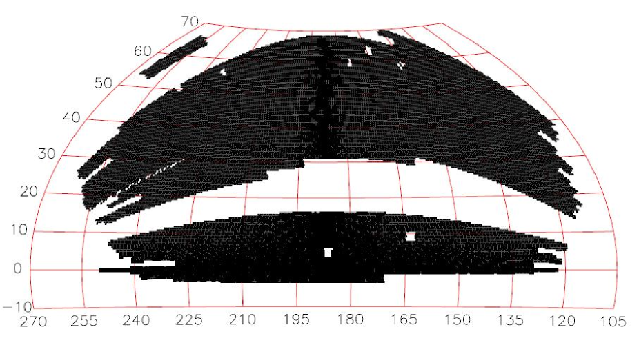
Figure 1: The angular coverage map of the NGP region of the SDSS DR4, which was analyzed in this study. The right ascension and declination values are plotted in degrees and an equal-area Aitoff projection is used. The total area of this survey region is $5{,}914$ deg². The dashed lines indicate constant Galactic latitudes of $45^{\circ}$ (the innermost pair), $30^{\circ}$ and $15^{\circ}$. There are several small gaps within the observed regions due to faults or poor-quality data.

We applied some star-galaxy separation criteria to the resulting catalogue (Collister et al. 2006). Firstly we made cuts based on galaxy angular size and the difference between the “p.s.f.” and model magnitudes. In addition, we trained our photometric-redshift neural network to improve the efficiency of star-galaxy separation. We introduced an additional parameter $\delta_{\rm sg}$ to the network such that $\delta_{\rm sg}=1$ if the training 2SLAQ object is a galaxy and $\delta_{\rm sg}=0$ if the object has been spectroscopically identified as a star. The network then output values of $\delta_{\rm sg}$ for each photometric object. These values form a continuous distribution between 0 and 1 and may be interpreted as a star-galaxy classification probability. Catalogue galaxies with low values of $\delta_{\rm sg}$ were then excluded from the clustering analysis. We chose the cut $\delta_{\rm sg}>0.2$, which reduced the level of stellar contamination to $\sim 1.5\%$ with the loss of only $\sim 0.1\%$ of the genuine galaxies. The final catalogue analyzed in this paper contains $644{,}903$ entries. In Section 4 we consider the effects on the power spectrum of varying the star-galaxy separation procedure.

2.2 Angular selection function

We measured the clustering of galaxies selected from the SDSS 4th Data Release (DR4) in the North Galactic Plane (NGP). We analyzed galaxies in the area bounded by right ascensions $110^{\circ}<\alpha<270^{\circ}$ and declinations $-5^{\circ}<\delta<70^{\circ}$. This area excludes the three SDSS stripes in the South Galactic Plane (stripes 76, 82 and 86) which contribute a small fraction of the surveyed area and which are widely spaced from the rest of the survey region.

We determined the angular selection function within the region $(110^{\circ}<\alpha<270^{\circ},-5^{\circ}<\delta<70^{\circ})$ using the coverage mask provided by the SDSS team (the files atStripeDef.par and tsChunk.dr4.best.par available via the web-page http://www.sdss.org/dr4/coverage). The publicly-available information includes the extent of the observations in each survey stripe and a list of holes due to faults or poor-quality data. This information is given in terms of SDSS “survey co-ordinates” ($\mu$ and $\nu$ for each stripe) which may be converted to right ascension and declination using the relations given on the web-page. This data was used to produce our initial window function by assigning “1” to the surveyed areas and “0” to the unsurveyed areas (Figure 1). The sky area encompassed by this window function is $5{,}914$ deg², mapping out a total cosmic volume $2.5\,h^{-3}$ Gpc³ across the redshift range $0.4<z<0.7$.

There are various effects which may cause the true angular selection function for the survey data to deviate from this binary coverage map (Scranton et al. 2005). These effects include: varying completeness in the overlap regions between survey stripes, dust extinction or seeing variations, incompleteness in the vicinity of very bright stars or galaxies, and systematic effects induced by star-galaxy separation. If left uncorrected, these effects may potentially cause a systematic error in the measured clustering pattern, particularly on large scales. We investigate the importance of these effects in Section 4 using an extensive series of tests. Our conclusion is that, as far as we can tell from these tests, the binary coverage map is an acceptable approximation in the galaxy magnitude range $17.5\leq i_{\rm deV}\leq 19.8$ analyzed in this study.

2.3 Photometric redshifts

We determined photometric redshift estimates for the LRG catalogue using the software package “ANNz” (Collister & Lahav 2004). In brief, artificial neural networks are applied to parameterize the relation between the galaxy redshift and the input information (principally the galaxy photometry, but other data such as the angular radius containing a given fraction of the galaxy flux can be readily included). The neural network is “trained” using a set of galaxies with known spectroscopic redshifts (in this case, a subset of the 2SLAQ database) by minimizing a “cost function” (essentially, the sum of the squared differences between the photometric and spectroscopic redshifts). After each training iteration, the cost function is also evaluated for a separate “validation” set of spectroscopic redshifts (a second subset of the 2SLAQ database) in order to avoid over-fitting to the training set given the presence of noise. The final photometric-redshift performance is objectively assessed by a third subset of the spectroscopic sample called the “evaluation” set. Further details on the ANNz software may be found in Collister & Lahav (2004).

For the input photometry we used the de-reddened $griz$-band “model magnitudes” of the SDSS galaxies, which provide the most robust colour estimates. We excluded the $u$-band photometry owing to concerns over a time-varying red leak in this filter that could potentially introduce systematic errors in the photometric redshifts as a function of galaxy position on the sky. In fact, irrespective of this concern, the $u$-band does not contribute any measurable benefit to the photometric redshift accuracy owing to the relatively low signal-to-noise ratio of the $u$-band photometry.

The resulting photometric redshifts for the conservative version of the catalogue analyzed in this paper, assessed using the spectroscopic evaluation set, possess a standard redshift error

$$\sigma_{z}\equiv\left[\overline{(\delta z)^{2}}-\left(\overline{\delta z}\right)^{2}\right]^{1/2}\approx 0.041$$ (1)

where $\delta z=z_{\rm phot}-z_{\rm spec}$, and do not suffer from any significant bias in the mean difference with respect to the spectroscopic redshifts, $\overline{\delta z}<0.001$ (considering galaxies in the range $0.4<z_{\rm spec}<0.7$, $0.4<z_{\rm phot}<0.7$ and $i_{\rm deV}<19.8$). The performance of our code is hence comparable to the results obtained for a similar sample of galaxies by Padmanabhan et al. (2005). Figure 2 is a scatter plot of photometric and spectroscopic redshifts in the range of interest. The principal systematic effect is that galaxies with $z_{\rm spec}<0.45$ are scattered up in photometric redshift such that there are very few galaxies with $z_{\rm phot}<0.45$. The robustness of the photometric redshifts worsens in the vicinity of $z\approx 0.4$ because the 4000Å  break enters a region of poor sensitivity between the $g$ and the $r$ bands. In addition, galaxies with $z_{\rm spec}>0.65$ are typically scattered down in redshift. Photometric redshift performance improves steadily with brightening magnitudes (and hence decreasing redshifts), reaching $\sigma_{z}\approx 0.02$ for the brightest galaxies. We refer the reader to Collister et al. (2006) for more discussion. We note that the small level of systematic photo-$z$ bias evident in Figure 2 is not a concern because it can be quantified using the spectroscopic redshift data and folded into our survey simulations.

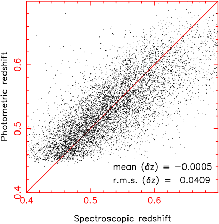
Figure 2: Comparison between the photometric redshift $z_{\rm phot}$ and spectroscopic redshift $z_{\rm spec}$ of galaxies in our evaluation set (for the conservative version of the catalogue analyzed in this paper). The mean and standard deviation of the quantity $\delta z=z_{\rm phot}-z_{\rm spec}$ are indicated.

Figure 3 is a plot of the distribution of spectroscopic redshifts in the evaluation set for galaxies binned in four photometric-redshift slices of width $\Delta z=0.05$ from $z=0.45$ to $z=0.65$. We find that these error distributions are well fitted by Gaussian distributions; the best-fitting values of the mean and standard deviation for the different slices are indicated in the Figure. These Gaussian functions are taken as our model for the redshift distribution of galaxies in each photo-$z$ slice when analyzing the galaxy clustering results. We repeated our cosmological analyses using the raw binned redshift distributions in each slice in place of the Gaussian fits, and found no significant difference in results. The number of galaxies with photometric redshifts outside the range $0.45<z<0.65$ is very small.

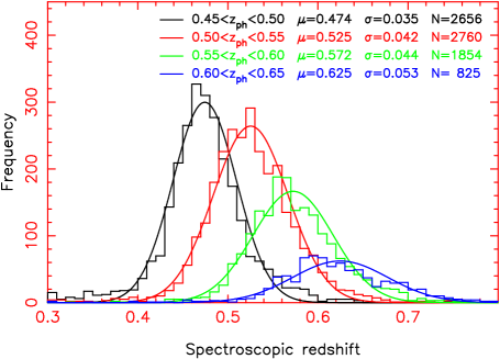
Figure 3: Gaussian fits to the spectroscopic redshift distribution of Luminous Red Galaxies in each of four photometric redshift slices analyzed in this study. The best-fitting Gaussian parameters $\mu$ and $\sigma$ are indicated, where $p(z)\propto\exp{\{-[(z-\mu)^{2}/2\sigma^{2}]\}}$. $N$ is the number of galaxies in the evaluation set used to measure the distribution in each slice.

The photometric redshift performance is sufficiently good that we can observe the clustering visually. Figure 4 plots the 2000 most luminous galaxies in the stripe $135^{\circ}<\alpha<235^{\circ}$, $0^{\circ}<\delta<10^{\circ}$ in each of a series of narrow redshift slices of width $\Delta z=0.03$. The characteristic patterns of large-scale structure may be readily discerned.

3 Measurement of the angular power spectrum

3.1 Method

A distribution of galaxies can be related to its angular power spectrum $C_{\ell}$ in two statistical steps. Firstly, the galaxy density field projected onto the sky, $\sigma(\theta,\phi)$, is expanded in terms of its spherical harmonic coefficients $a_{\ell,m}$:

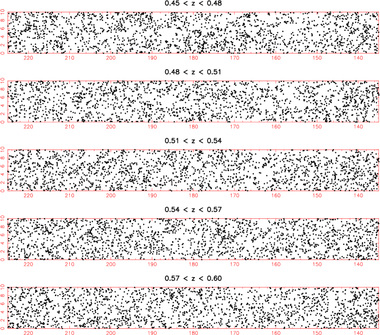
Figure 4: The locations of the 2000 most luminous galaxies in each of a series of photometric redshift slices of width $\Delta z=0.03$ in a narrow survey stripe. The characteristic patterns of large-scale structure may be observed. The axes are right ascension and declination in decimal degrees.

$$\sigma(\theta,\phi)=\sum_{\ell=0}^{\infty}\sum_{m=-\ell}^{\ell}a_{\ell,m}\,Y_{\ell,m}(\theta,\phi)$$ (2)

where $Y_{\ell,m}$ are the usual spherical harmonic functions. Secondly, galaxy positions are generated in a Poisson process as a (possibly biased) realization of this density field. The angular power spectrum $C_{\ell}$ prescribes the expectation values of the spherical harmonic coefficients in the first step of this model. It is defined over many realizations of the density field (indicated by angled brackets) as:

$$<|a_{\ell,m}|^{2}>=C_{\ell}\,.$$ (3)

The measurement of the angular power spectrum from a set of discrete galaxy positions has been discussed by many authors. The available techniques can be crudely divided into two principal approaches. Firstly, the power spectrum can be derived by direct spherical harmonic estimation, in which the harmonic coefficients are calculated by summation over the galaxy angular positions (e.g. Peebles 1973; Scharf et al. 1992; Wright et al. 1994; Wandelt, Hivon & Gorski 2001). Secondly, a maximum likelihood approach can be utilized (similar to those commonly employed for the analysis of CMB temperature and polarization maps). Examples of the application of maximum likelihood methods to galaxy clustering measurements are the papers by Efstathiou & Moody (2001); Huterer, Knox & Nichol (2001) and Tegmark et al. (2002).

We used the technique of spherical harmonic estimation in the present study. We give a brief summary of the method here, referring the reader to Blake, Ferreira & Borrill (2004) for more details. The spherical harmonic coefficients of a density field for a completely observed sky may be estimated by summing over the $N$ galaxy positions $(\theta_{i},\phi_{i})$:

$$A_{\ell,m}=\sum_{i=1}^{N}Y_{\ell,m}^{*}(\theta_{i},\phi_{i})$$ (4)

The estimator for the angular power spectrum is then

$$C_{\ell,m}^{\rm obs}=|A_{\ell,m}|^{2}-N/\Delta\Omega$$ (5)

such that $<C_{\ell,m}^{\rm obs}>=C_{\ell}$. $\Delta\Omega$ is the total survey area, which is $4\pi$ for a complete sky. The discreteness of the distribution causes the correction term “$-N/\Delta\Omega$”. For a given multipole $\ell$ there are $2\ell+1$ different estimators of $C_{\ell}$ corresponding to $m=-\ell,-\ell+1,...,-1,0,1,...,\ell$.

For an incomplete sky, these equations must be corrected for the unsurveyed regions, such that an estimate of $C_{\ell}$ is

$$C_{\ell,m}^{\rm obs}=\frac{|A_{\ell,m}-(N/\Delta\Omega)\,I_{\ell,m}|^{2}}{J_{\ell,m}}-\frac{N}{\Delta\Omega}$$ (6)

(e.g. Peebles 1973 equation 50) where

$$I_{\ell,m}=\int_{\Delta\Omega}Y_{\ell,m}^{*}\,d\Omega$$ (7)

$$J_{\ell,m}=\int_{\Delta\Omega}|Y_{\ell,m}|^{2}\,d\Omega$$ (8)

where the integrals are performed over the survey area $\Delta\Omega$, and are determined in our analysis by numerical integration. For the SDSS area analyzed in this study (Figure 1), $\Delta\Omega/4\pi=0.143$.

We determined the observed angular power spectrum for the $\ell$th multipole, $C_{\ell}^{\rm obs}$, by averaging equation 6 over $m$:

$$C_{\ell}^{\rm obs}=\frac{\sum_{m=-\ell}^{\ell}C_{\ell,m}^{\rm obs}}{2\ell+1}$$ (9)

The partial sky coverage has the effect of convolving the harmonic coefficients such that the measured angular power spectrum at multipole $\ell$ depends on a range of multipoles $\ell^{\prime}$ of the underlying power spectrum:

$$<C_{\ell}^{\rm obs}>=\sum_{\ell^{\prime}}R_{\ell,\ell^{\prime}}\,C_{\ell^{\prime}}$$ (10)

The “mixing matrix” $R_{\ell,\ell^{\prime}}$ may be determined from the angular power spectrum $W_{\ell}$ of the survey window function:

$$R_{\ell,\ell^{\prime}}=\frac{2\ell^{\prime}+1}{4\pi}\sum_{\ell^{\prime\prime}}(2\ell^{\prime\prime}+1)\,W_{\ell^{\prime\prime}}\left(\begin{array}[]{ccc}\ell&\ell^{\prime}&\ell^{\prime\prime}\\ 0&0&0\end{array}\right)^{2}$$ (11)

where the matrix in equation 11 is a Wigner 3-$j$ symbol and

$$W_{\ell}=\frac{\sum_{m=-\ell}^{\ell}|I_{\ell,m}|^{2}}{2\ell+1}$$ (12)

(e.g. Hivon et al. 2002; Deligny et al. 2004). In Figure 5 we plot normalized values of the mixing matrix $R_{\ell,\ell^{\prime}}$ evaluated using equation 11, corresponding to the SDSS DR4 geometry displayed in Figure 1, for multipole $\ell=200$ as a function of $\ell^{\prime}$. The convolution function $R_{200,\ell^{\prime}}$ is sharply peaked, dropping to $10\%$ of its peak value for an offset $\Delta\ell=4$ from the peak. The shape of this function is largely insensitive to the choice of $\ell=200$: to a very good approximation, changing this value of $\ell$ only causes a translation of the function along the $\ell^{\prime}$-axis.

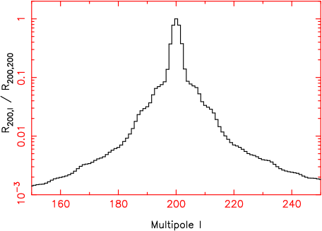
Figure 5: The mixing matrix $R_{\ell,\ell^{\prime}}$ for multipole $\ell=200$ as a function of $\ell^{\prime}$, indicating the range of multipoles correlated by the survey window function effects (see equations 10 and 11 for the definition of $R_{\ell,\ell^{\prime}}$).

We averaged the measured angular power spectra in multipole bands of width $\Delta\ell=10$. It can be seen from the foregoing argument that these bands are approximately statistically independent (correlated at a level below $10\%$) and we neglected the residual correlations. We determined the angular power spectrum up to a maximum multipole $\ell_{\rm max}=500$ (in Section 3.4 we limit the range of multipoles to be fitted by our theoretical model in accordance with the approximate extent of the linear clustering regime).

3.2 Error determination

We compared various different determinations of the statistical error $\sigma(C_{\ell})$ in our measurement of the angular power spectrum. Firstly, the application of Gaussian statistics leads to a simple analytical approximation (e.g. Dodelson 2003 p.342 eq.11.27):

$$\sigma(C_{\ell})=\sqrt{\frac{2}{f_{\rm sky}(2\ell+1)}}\left(C_{\ell}+\frac{1}{N/\Delta\Omega}\right)$$ (13)

where $N/\Delta\Omega$ is the average source density (in units of sr^-1) and $f_{\rm sky}$ denotes the fraction of sky covered by the survey. The structure of this equation can be readily understood in crude terms. The contribution to the error for each value of $m$ consists of a cosmic variance term ($C_{\ell}$) and a shot noise term [$(N/\Delta\Omega)^{-1}$]. The averaging over $m$ reduces the variance by a factor $2\ell+1$. The fraction of sky covered by the survey enters as $\sigma(C_{\ell})\propto 1/\sqrt{f_{\rm sky}}$. (If the observed sky area is halved and just one of these sub-areas is analyzed, we would expect the standard deviation of the measurement to increase by a factor $\sqrt{2}$, under the approximation that the two sub-areas are independent.)

We used equation 13 in our cosmological parameter fitting. We note that the value of $C_{\ell}$ in the equation could correspond to either the measured power or the model power at the multipole in question. In our treatment we used the model angular power spectrum for each combination of parameters to re-derive the statistical error and assess the goodness-of-fit of that set of parameters.

Estimating the measurement error using equation 13 involves at least two approximations:

• The effects of the survey window function are encapsulated in just one quantity $f_{\rm sky}$, thus equation 13 is not likely to be valid for multipoles $\ell$ corresponding to angular scales $\theta\sim 180^{\circ}/\ell$ which are similar to or larger than those defining the structure of the window function (for which edge effects, i.e. the distribution of the survey area, are likely to be important).

• Gaussian statistics are assumed, thus equation 13 is not likely to be valid in the regime of non-linear clustering.

However, it may be hoped that equation 13 is a good approximation for multipoles $\ell$ corresponding to angular scales $\theta$ smaller than the typical structure of the window function ($\theta<2.5^{\circ}$ in our case), but large enough that the corresponding spatial scales lie in the (quasi-)linear regime where Gaussian statistics should apply. This turns out to be the case for our analysis.

In order to test the validity of equation 13, we estimated the error in the angular power spectrum using two additional methods:

• We generated Monte Carlo realizations of galaxy distributions consistent with a model angular power spectrum similar to that measured for the real data, using the same survey window function as plotted in Figure 1. For each realization we calculated the density field $\sigma(\theta,\phi)$ (over a fine grid of pixels) by evaluating equation 2 for a set of spherical harmonic coefficients corresponding to a Gaussian realization of the underlying $C_{\ell}$ spectrum. We then produced a catalogue of discrete galaxies as a Poisson realization of this density field, and measured the angular power spectrum using the same techniques utilized for the real survey data. The scatter of the measured power spectra across these Monte Carlo realizations will include the full effects of the survey window function, unlike equation 13, and this investigation is therefore designed to assess the approximation of using the single quantity $f_{\rm sky}$ to represent these effects.

• Using a “boot-strap” approach, we divided the observed survey area into many $10\times 10$ deg patches (the choice of patch size is a compromise between capturing a sufficient number of large-scale power spectrum modes within a single patch, and ensuring there are enough patches across the sky to permit reasonable statistics). We measured the angular power spectrum of the galaxies within each patch using a flat-sky approximation (i.e., by taking a 2D Fast Fourier transform of the overdensity field $\delta_{x}$ and evaluating the 2D power spectrum $P_{2}(k)\equiv|\delta_{k}|^{2}$. In the small-angle approximation, $C_{\ell}=P_{2}(\ell)$.) The standard deviation of the power spectra across these patches is not sensitive to the global survey window function, but should trace non-Gaussian effects present in the data, thereby assessing the approximation of Gaussianity in equation 13.

In Figure 6 we plot the ratio of the angular power spectrum error measured by these two techniques to the prediction of equation 13. It can be seen that equation 13 is a good approximation for the standard deviation for the scales of interest, and it is used in our analysis. Section 3.3.2 presents an additional test for the Gaussianity of the clustering fluctuations.

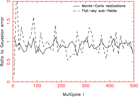
Figure 6: The ratio of the error in the angular power spectrum measurement to the Gaussian prediction of equation 13 determined by two different techniques: firstly by Monte Carlo realizations (the solid line), and secondly by an analysis dividing the survey area into many independent patches (the dashed line). The Gaussian prediction is a good approximation for the scales of interest. The “spikiness” of the dashed line is caused by the poor signal-to-noise ratio of the measurements in the $10\times 10$ deg patches, but the average behaviour is in good agreement with the Gaussian prediction.

3.3 Results

3.3.1 Angular power spectra

We measured the angular power spectrum of the LRGs (using the estimator defined by equations 6 to 9) in four photometric redshift slices of width $\Delta z=0.05$ between $z=0.45$ and $z=0.65$. The results, averaged in multipole bands of width $\Delta\ell=10$, are listed in Table 1, together with the Gaussian errors of equation 13 (divided by $\sqrt{\Delta\ell}$ to account for the binning). For the purposes of this Table the measured power spectra are used to assign the errors with equation 13. When fitting cosmological models to these power spectra in Section 3.4, the model power spectra are used to determine the Gaussian errors. The surface densities $N/\Delta\Omega$ of galaxies in the four slices are $(35.7,29.1,18.8,8.7)$ deg^-2. The results are also plotted in the left-hand panels of Figure 10.

3.3.2 Probability distribution of $A_{\ell,m}$

The distribution of values of $A_{\ell,m}$ (the estimated spherical harmonic coefficients defined by equation 4) is an interesting probe of the galaxy distribution (Peebles 1973; Hauser & Peebles 1973). Consider first an unclustered distribution of points with surface density $N/\Delta\Omega$ over a full sky. The central limit theorem ensures that the real and imaginary parts of $A_{\ell,m}=\sum_{i}Y_{\ell,m}^{*}(i)$ are drawn independently from Gaussian distributions such that the normalization satisfies $<|A_{\ell,m}|^{2}>=N/\Delta\Omega$. It is then easy to show that $x=|A_{\ell,m}|^{2}$ has an exponential probability distribution $P(x)$ for $m\neq 0$:

$$P(x)\,dx=\frac{\exp{(-x/\alpha)}}{\alpha}dx$$ (14)

where $\alpha=N/\Delta\Omega$. For a partial sky, $|A_{\ell,m}|^{2}$ should be replaced by $x=|A_{\ell,m}-(N/\Delta\Omega)I_{\ell,m}|^{2}/J_{\ell,m}$. For a clustered distribution, $\alpha$ assumes the value $(N/\Delta\Omega)+C_{\ell}$ and equation 14 holds if each Fourier component has a randomly-assigned phase. The validity of equation 14 is therefore a good cross-check of the applicability of the linear regime, for which the random-phase assumption should apply (Chiang & Coles 2000).

Figure 7 plots the distribution of the quantity $x$ for harmonic coefficients in the range $1\leq m\leq\ell$ in six different multipole bands of width $\Delta\ell=10$, for the first of the photometric redshift slices defined above ($0.45<z<0.5$). We also display the expected probability distribution for random-phase statistics, deriving the quantity $\alpha=(N/\Delta\Omega)+C_{\ell}$ from the galaxy surface density together with the measured strength of the angular power spectrum in the multipole band. We find that the observed distribution of harmonic coefficients is a very good match to the random-phase prediction even for the highest multipoles considered ($\ell=300$).

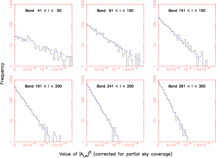
Figure 7: The distribution of values of $|A_{\ell,m}|^{2}$ (corrected for partial sky coverage) for harmonic coefficients $1\leq m\leq\ell$ in six multipole bands of width $\Delta\ell=10$ for the photometric redshift slice $0.45<z<0.5$. The dashed lines are the predictions of random-phase statistics based on the observed strength of the power spectrum due to clustering and shot noise. The slope of this model changes across the six panels due to the varying amplitude of the angular power spectrum.

Table 1: The angular power spectrum measurements in four photometric redshift slices of width $\Delta z=0.05$ between $z=0.45$ and $z=0.65$. This table lists the values of $10^{5}\times C_{\ell}$ and the corresponding Gaussian error in multipole bands of width $\Delta\ell=10$. The errors $\sigma(C_{\ell})$ are determined for the purposes of this Table by substituting the measured values of $C_{\ell}$ in equation 13 and not from the best-fitting power spectrum model.

$\ell$	Slice 1		Slice 2		Slice 3		Slice 4
	$C_{\ell}$	$\sigma(C_{\ell})$	$C_{\ell}$	$\sigma(C_{\ell})$	$C_{\ell}$	$\sigma(C_{\ell})$	$C_{\ell}$	$\sigma(C_{\ell})$
6	19.400	7.880	12.600	5.050	19.000	9.600	37.200	24.300
16	14.500	3.390	9.510	2.400	12.000	3.000	10.800	3.470
26	8.980	1.770	7.680	1.520	10.900	2.110	9.770	2.250
36	7.930	1.240	7.600	1.260	7.490	1.390	6.150	1.420
46	6.400	0.900	5.960	0.871	5.900	0.933	6.080	1.200
56	5.290	0.694	4.360	0.614	5.010	0.749	4.150	0.863
66	5.240	0.632	4.740	0.597	4.360	0.622	4.260	0.811
76	4.450	0.517	5.360	0.629	3.870	0.530	3.570	0.690
86	3.580	0.409	4.300	0.484	4.280	0.536	3.280	0.617
96	3.390	0.364	3.630	0.401	3.600	0.448	2.790	0.540
106	3.370	0.345	3.250	0.350	3.370	0.408	2.740	0.510
116	2.860	0.289	2.830	0.302	2.560	0.331	2.980	0.508
126	2.350	0.239	2.290	0.250	2.020	0.272	2.050	0.417
136	2.260	0.224	2.160	0.231	2.220	0.278	2.620	0.442
146	2.300	0.219	1.880	0.202	2.070	0.259	1.580	0.357
156	2.130	0.200	1.890	0.197	1.760	0.227	1.510	0.339
166	1.880	0.178	1.420	0.160	1.640	0.212	1.750	0.342
176	1.580	0.153	1.770	0.178	1.580	0.203	1.600	0.323
186	1.730	0.159	1.620	0.164	1.340	0.182	1.180	0.289
196	1.320	0.131	1.200	0.134	1.570	0.191	1.390	0.294
206	1.290	0.125	1.190	0.130	1.200	0.165	1.320	0.282
216	1.300	0.122	1.200	0.128	1.290	0.166	1.290	0.275
226	1.160	0.112	1.180	0.124	1.240	0.159	1.080	0.256
236	1.180	0.111	1.120	0.118	1.130	0.150	0.775	0.234
246	0.948	0.096	0.841	0.101	0.853	0.132	1.070	0.245
256	1.050	0.100	0.909	0.102	0.925	0.133	0.890	0.230
266	0.972	0.094	0.915	0.101	0.933	0.131	0.592	0.212
276	0.815	0.084	0.949	0.101	0.899	0.127	0.796	0.218
286	0.702	0.077	0.821	0.092	1.030	0.131	1.130	0.230
296	0.759	0.079	0.629	0.081	0.712	0.113	0.893	0.215
306	0.809	0.079	0.776	0.087	0.578	0.105	0.535	0.194
316	0.819	0.079	0.783	0.086	0.612	0.105	0.762	0.202
326	0.794	0.076	0.715	0.082	0.679	0.107	0.646	0.193
336	0.667	0.069	0.694	0.079	0.761	0.109	0.722	0.194
346	0.726	0.071	0.701	0.078	0.588	0.099	0.904	0.199
356	0.649	0.067	0.677	0.076	0.692	0.103	0.841	0.193
366	0.593	0.063	0.574	0.071	0.623	0.098	0.659	0.183
376	0.645	0.065	0.722	0.076	0.498	0.092	0.673	0.181
386	0.568	0.061	0.518	0.067	0.490	0.090	0.457	0.169
396	0.595	0.061	0.600	0.069	0.625	0.094	0.635	0.175
406	0.547	0.058	0.546	0.066	0.514	0.089	0.622	0.172
416	0.392	0.051	0.499	0.063	0.522	0.088	0.487	0.164
426	0.584	0.058	0.566	0.065	0.454	0.084	0.433	0.160
436	0.489	0.054	0.529	0.063	0.623	0.090	0.509	0.161
446	0.521	0.054	0.432	0.059	0.461	0.083	0.599	0.163
456	0.444	0.051	0.349	0.054	0.393	0.079	0.661	0.164
466	0.452	0.051	0.361	0.054	0.515	0.083	0.566	0.159
476	0.414	0.048	0.454	0.058	0.514	0.082	0.416	0.151
486	0.397	0.047	0.473	0.058	0.322	0.074	0.352	0.147
496	0.512	0.051	0.413	0.055	0.408	0.076	0.512	0.152

3.4 Cosmological parameter fits

3.4.1 Independent redshift slices

The angular power spectrum $C_{\ell}$ is a projection of the spatial power spectrum of fluctuations at different redshifts $z$, $P(k,z)$, where $k$ is a co-moving wavenumber. The equation for the projection is:

$$C_{\ell}=\frac{2\,b^{2}}{\pi}\int P_{0}(k)\,g_{\ell}(k)^{2}\,dk$$ (15)

where $P(k,z)=P_{0}(k)\,D(z)^{2}$, with $D(z)$ the linear growth factor at redshift $z$. We note that this decomposition of $P(k,z)$ is strictly only valid in linear theory, and its application at smaller scales is an approximation. We have assumed a scale-independent bias factor $b$ at redshift $z$ for the galaxies with respect to the underlying matter fluctuations.

The kernel $g_{\ell}(k)$ is given by (neglecting redshift-space distortions):

$$g_{\ell}(k)=\int_{0}^{\infty}j_{\ell}(u)\,f(u/k)\,du\,.$$ (16)

Here, $j_{\ell}(x)$ is the spherical Bessel function and $f(x)$ depends on the radial distribution of the sources as

$$f[z(x)]=p(z)\,D(z)\left(\frac{dx}{dz}\right)^{-1}$$ (17)

where $x(z)$ is the co-moving radial co-ordinate at redshift $z$, and $p(z)$ is the redshift probability distribution of the sources, normalized such that $\int p(z)\,dz=1$ (see e.g. Huterer, Knox & Nichol 2001; Tegmark et al. 2002; Blake et al. 2004). A good approximation for these equations which is valid for moderately large $\ell\ga 50$ is:

$$C_{\ell}=b^{2}\int P(k=\ell/x,z)\,x(z)^{-2}\,p(z)^{2}\,\left(\frac{dx}{dz}\right)^{-1}dz\,.$$ (18)

The angular power spectrum will be modified by redshift-space distortions on large scales. These distortions significantly affect the amplitude of the projected power spectrum on large scales $\ell\la 50$, owing to the relative narrowness of each redshift slice. The amplitude of the redshift-space distortions is controlled by a parameter $\beta(z)\approx\Omega_{\rm m}(z)^{0.6}/b(z)$, where the quantities on the right-hand side of the equation are evaluated at the centre of each redshift slice of our analysis. The effect is to introduce an additional term to the kernel of equation 16 such that it becomes $g_{\ell}(k)+g^{\beta}_{\ell}(k)$ where:

$$g^{\beta}_{\ell}(k)=\frac{\beta}{k}\int_{0}^{\infty}j_{\ell}^{\prime}(u)\,f^{\prime}(u/k)\,du$$ (19)

(Fisher, Scharf & Lahav 1994; Padmanabhan et al. 2006 eq.26).

We can use these expressions to fit cosmological parameters to the angular power spectrum data in each redshift slice. The cosmological parameters determine both the power spectrum of fluctuations $P(k,z)$ and the co-moving distance $x(z)$ in the above equations. For the redshift distribution of the sources $p(z)$ we used the Gaussian functions fitted to the training set data (see Figure 3). We derived model spatial power spectra using the “CAMB” software package (Lewis, Challinor & Lasenby 2000) which is based on CMBFAST (Seljak & Zaldarriaga 1996), including corrections for non-linear growth of structure using the fitting formulae of Smith et al. (2003) (“halofit=1” in CAMB). We outputted power spectra at $z=0.55$ (the mean redshift under analysis) and scaled these spectra to other redshifts using the linear growth factor $D(z)^{2}$.

For low multipoles $\ell$, we calculated the model angular power spectrum for a given set of cosmological parameters using the exact expression of equation 15, incorporating redshift-space distortions. For reasons of speed, we substituted the expression of equation 18 at higher values of $\ell$ when the approximation became acceptable. Before comparing each model with observations we convolved it with the survey window function using equation 10. Figure 8 displays the modifications to the angular power spectrum caused by redshift-space distortions and by the survey window function for an example case. Figure 9 plots the kernel $g_{\ell}(k)$ appearing in equation 15 (including the redshift-space distortion contribution) for various multipoles $\ell$. This kernel controls which physical scales $k$ (in Fourier space) contribute power to a clustering measurement at a particular multipole $\ell$. It can be seen that the projection at any given multipole involves a relatively small range $\Delta k$ of scales owing to the narrowness of the photometric-redshift slice $\Delta x$ in co-ordinate space (the approximate range is $\Delta k/k=\Delta x/x$, where $k=\ell/x$).

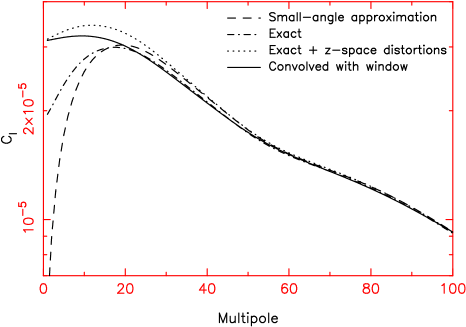
Figure 8: The model angular power spectrum for the photometric redshift slice $0.45<z<0.5$ under various assumptions: (1) the small-angle approximation (equation 18); (2) the exact expression in real space (equation 15 with the kernel of equation 16); (3) after the inclusion of redshift-space distortions (with the addition of the kernel of equation 19); (4) after convolution with the survey window function using equation 10. The assumed cosmological parameters are $\Omega_{\rm m}=0.26$, $f_{\rm b}=0.16$, $h=0.75$, $\sigma_{8}=1$, $\beta=0.3$. The small-angle approximation is acceptable for the multipole range $\ell\ga 50$; at low multipoles the results differ very significantly.

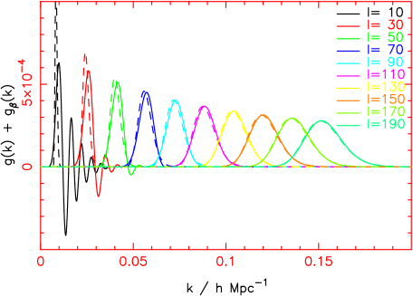
Figure 9: The kernel $g_{\ell}(k)+g^{\beta}_{\ell}(k)$ appearing in equation 15 for various multipoles $\ell$. This plot indicates the range of Fourier scales $k$ contributing to angular power at a given multipole $\ell$ (each solid line is for a different value of $\ell$ increasing from left to right). The dashed line indicates the kernel implied by the small-angle-approximation of equation 18. The assumed cosmological parameters are $\Omega_{\rm m}=0.26$, $f_{\rm b}=0.16$, $h=0.75$, $\sigma_{8}=1$, $\beta=0.3$. We again see that the small-angle approximation is acceptable for the multipole range $\ell\ga 50$.

The galaxy clustering pattern is well-known to be sensitive principally to the quantity $\Omega_{\rm m}H_{0}$ (where $\Omega_{\rm m}$ is the matter density and $H_{0}$ is Hubble’s constant), and secondarily to the baryon fraction $\Omega_{\rm b}/\Omega_{\rm m}$. For our initial investigation we fixed the values of the Hubble constant $H_{0}=75$ km s^-1 Mpc^-1 and the tilt of the primordial power spectrum $n_{\rm scalar}=1$ (e.g. following Cole et al. 2005; we consider variations in $H_{0}$ and $n_{\rm scalar}$ in Section 3.4.2). We then varied over a grid the matter density $\Omega_{\rm m}$, the baryon fraction $f_{\rm b}=\Omega_{\rm b}/\Omega_{\rm m}$, the present-day normalization of the power spectrum $\sigma_{8}$, and the constant galaxy bias factor $b$. In the linear regime $\sigma_{8}$ and $b$ are degenerate, but to allow for any contribution from quasi-linear modes we marginalized over both separately, using a flat prior $0.7\leq\sigma_{8}\leq 1.1$. We determined the co-moving distance $x(z)$ assuming a flat universe with the remainder of the energy density provided by a cosmological constant. We calculated the value of the redshift-distortion parameter at each model grid point by assuming $\beta=\Omega_{\rm m}(z_{0})^{0.6}/b$, where $z_{0}$ is the central redshift of the photo-$z$ slice.

We determined the relative likelihood of each model using:

$${\rm Likelihood}\propto|M|^{-1/2}\exp{[-(d^{T}M^{-1}d)/2]}$$ (20)

where $d=C_{\ell,{\rm obs}}-C_{\ell,{\rm mod}}$ is the vector of differences between the model predictions and the data points in each band of multipoles; and $M$ is the covariance matrix, evaluated for the particular model at the grid point using equation 13 (the chi-squared statistic is $\chi^{2}=d^{T}M^{-1}d$). Since we are neglecting correlations between multipole bands, the covariance matrix here is diagonal.

We assumed that power spectrum modes with spatial scales $k\la 0.2\,h$ Mpc^-1 could be modelled via equation 18 using a scale-independent bias factor $b$ (this is comparable to the smallest scales fitted in lower-redshift surveys – $k_{\rm max}\approx 0.15\,h$ Mpc^-1 in Percival et al. 2001 and $k_{\rm max}\approx 0.2\,h$ Mpc^-1 in Tegmark et al. 2004a). We estimated the equivalent maximum multipole of the angular power spectrum using the fact that at redshift $z$, a multipole $\ell$ probes spatial power on scales of roughly $k=\ell/r(z)$ (see equation 18 and Figure 9). This corresponds to $\ell_{\rm max}\approx 300$ at our mean redshift $z\approx 0.55$ and hence for each redshift slice we fitted our models to only the first 30 multipole bands of width $\Delta\ell=10$. Our placement of the non-linear transition at these angular scales is justified in Figure 10 by the small differences for $\ell<\ell_{\rm max}$ between the best-fitting non-linear power spectrum in each slice (generated by “halofit = 1” in CAMB) and the corresponding linear power spectrum with the same cosmological parameters (generated by “halofit = 0” in CAMB).

Table 2: Best-fitting values of the cosmological parameters for the modelling of the angular power spectra for multipoles $\ell\leq\ell_{\rm max}=300$ in the four photometric redshift slices. The best-fitting values and errors for $\Omega_{\rm m}$ and $f_{\rm b}=\Omega_{\rm b}/\Omega_{\rm m}$ are obtained by marginalizing over the other three parameters, including $\sigma_{8}$ and $b$. The values of the Hubble parameter $h$ and the tilt of the primordial power spectrum $n_{\rm scalar}$ are both held fixed in each analysis at the values given in the Table. The best-fitting values of the linear bias $b$ are quoted assuming $\sigma_{8}=1$. We also quote the value of the $\chi^{2}$ statistic for the best-fitting model and the number of degrees of freedom (d.o.f.) in each case, as well as the average galaxy absolute magnitude $M_{i}$. The combined measurements of all four slices are obtained by calculating a covariance matrix between redshift slices as described in the text.

Slice	$h$ (fixed)	$n_{\rm scalar}$ (fixed)	$\Omega_{\rm m}$	$f_{\rm b}$	$b$	$M_{i}-5$ log${}_{10}h$	$\chi^{2}$	d.o.f.
$0.45<z<0.5$	0.75	1.00	$0.28\pm 0.05$	$0.16\pm 0.06$	$1.51\pm 0.03$	$-22.45$	18.8	26
$0.5<z<0.55$	0.75	1.00	$0.26\pm 0.04$	$0.14\pm 0.06$	$1.68\pm 0.05$	$-22.67$	22.4	26
$0.55<z<0.6$	0.75	1.00	$0.24\pm 0.04$	$0.18\pm 0.06$	$1.74\pm 0.06$	$-22.92$	18.7	26
$0.6<z<0.65$	0.75	1.00	$0.28\pm 0.06$	$0.20\pm 0.07$	$1.95\pm 0.12$	$-23.17$	14.8	26
Combined	0.75	1.00	$0.26\pm 0.031$	$0.16\pm 0.036$			82.1	113
	0.7	1.00	$0.28\pm 0.032$	$0.16\pm 0.038$			82.3	113
	0.75	0.95	$0.28\pm 0.031$	$0.16\pm 0.039$			81.9	113

The best-fitting values of $\Omega_{\rm m}$ and $f_{\rm b}$ at each redshift, marginalizing over the other three parameters including $\sigma_{8}$ and $b$, are listed in Table 2. The results – $\Omega_{\rm m}\approx 0.27\pm 0.05$ and $f_{\rm b}\approx 0.17\pm 0.06$ – are consistent across the redshift slices. Our measurement of $\sigma_{8}$ is weak because we are restricting ourselves mainly to the linear clustering regime, where $\sigma_{8}$ and $b$ are largely degenerate. In Table 2 we quote the best-fitting values of $b$ in each redshift slice assuming $\sigma_{8}=1$. We find $1.5<b<1.9$, with this high bias reflecting the fact that LRGs prefer denser environments (e.g. Zehavi et al. 2005). We note that (in the linear regime) these bias measurements should be interpreted as constraints on the product $\sigma_{8}\times b$.

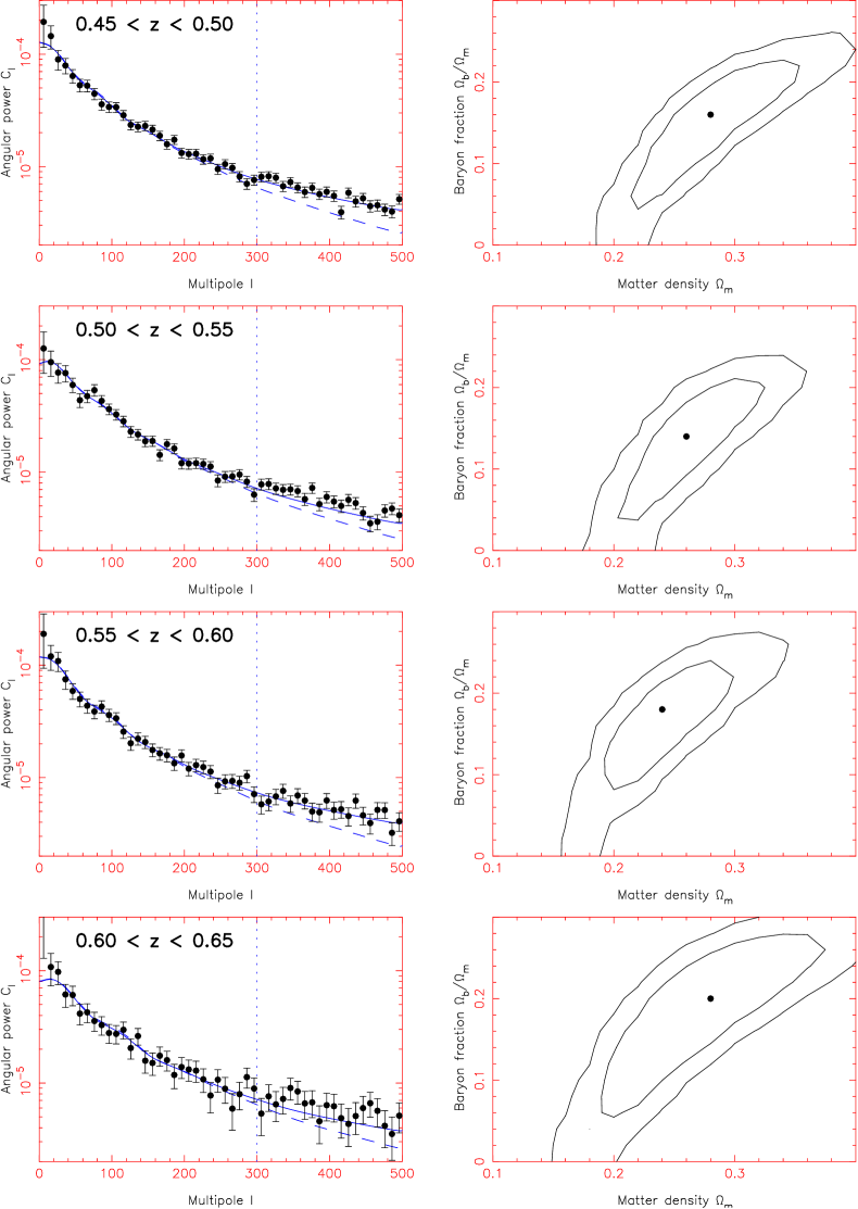
Figure 10: Each row of this Figure corresponds to a different photometric redshift slice, indicated by the caption. The left-hand column plots the angular power spectrum data (binned in multipole bands of width $\Delta\ell=10$) and the best-fitting model in each case (solid line) including both redshift-space distortions and convolution with the survey window function. The dashed line indicates a model with the same cosmological parameters but excluding the non-linear correction. The vertical dotted line indicates the range of multipoles we used in our fitting, $\ell<\ell_{\rm max}=300$. This corresponds to an estimate of the extent of the linear regime: spatial scales $k\la 0.2\,h$ Mpc^-1. The right-hand column displays 1-$\sigma$ and 2-$\sigma$ probability contours in the plane of $\Omega_{\rm b}/\Omega_{\rm m}$ and $\Omega_{\rm m}$, marginalizing over $\sigma_{8}$ and $b$. The solid circle indicates the best-fitting parameter combination in each case. The cross displays the best-fitting result when the four redshift slices are combined with appropriate covariances.

The bias systematically increases with redshift for two reasons:

1. Galaxies in more distant redshift slices are preferentially more luminous (owing to the fixed apparent magnitude threshold) and hence more strongly clustered (e.g. Norberg et al. 2002). In Table 2 we list the average absolute $i$-band magnitude $M_{i}$ of galaxies in each redshift slice, calculated using a K-correction obtained from a standard Luminous Red Galaxy template.

2. In standard models of the evolution of galaxy clustering, the bias factor of a class of galaxies increases with redshift in opposition to the decreasing linear growth factor, in order to reproduce the observed approximate constancy of the small-scale clustering length (e.g. Magliocchetti et al. 2000; Lahav et al. 2002).

In Figure 10 we plot the measured angular power spectra in the four redshift slices together with the cosmological parameter fits. Each row corresponds to a different redshift slice as indicated. The left-hand column displays the data points and the best-fitting models (solid line). The dashed lines illustrate the corresponding power spectrum models with the same cosmological parameters but omitting the non-linear corrections. The difference between these curves indicates the importance of the non-linear correction. The vertical dotted line indicates the position of the maximum multipole we used in our fitting, $\ell_{\rm max}=300$. The right-hand column plots 1-$\sigma$ and 2-$\sigma$ probability contours in the plane of $f_{\rm b}$ and $\Omega_{\rm m}$, marginalizing over $\sigma_{8}$ and $b$.

In all redshift slices the best models produce good fits to the shape of the clustering pattern over scales $\ell\leq\ell_{\rm max}=300$, as indicated by the acceptable values of $\chi^{2}$ listed in Table 2. In fact, the model generally remains a good match to the data for smaller scales $\ell>300$ which are not used in the fitting. At low multipoles there is a visual suggestion of a small excess (1-$\sigma$) of measured power with respect to the model prediction, but this statement lacks statistical significance.

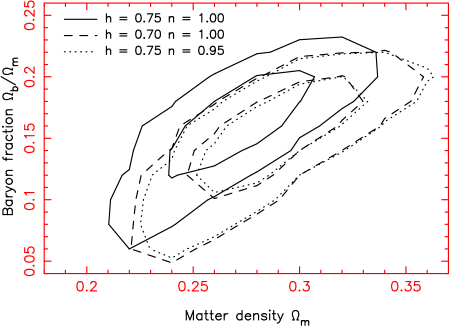
Figure 11: The probability distribution for the cosmological parameters $\Omega_{\rm m}$ and $\Omega_{\rm b}/\Omega_{\rm m}$ combining the four redshift slices using a full covariance matrix, and marginalizing over $\sigma_{8}$ and the four linear bias parameters. 1-$\sigma$ and 2-$\sigma$ contours are displayed. The solid and dashed contours assume $H_{0}=75$ and $70$ km s^-1 Mpc^-1, respectively.

3.4.2 Combined redshift slices

The cosmological results from different redshift slices are not independent, because galaxies sampling the same cosmic variance are scattered between slices by the photometric redshift errors. Therefore we cannot combine the results from the different redshift slices by simply multiplying together the four probability maps in Figure 10. Instead, we derived a full covariance matrix between the measurements of the angular power spectrum in multipole bands in all four redshift slices.

Since different multipole bands are uncorrelated within each redshift slice (to a good approximation), the covariance matrix has a simple structure of non-zero diagonals with entries for multipoles $\ell_{i}=\ell_{j}$ for redshift slices $i$ and $j$. These covariances are given by

$$<C^{i}_{\ell}\,C^{j}_{\ell}>-<C^{i}_{\ell}><C^{j}_{\ell}>=\frac{2}{f_{\rm sky}(2\ell+1)}\,C^{i,j}_{\ell}$$ (21)

using the same Gaussian approximation as equation 13. Here, $C^{i,j}_{\ell}$ is the cross angular power spectrum between the two redshift slices. This can be determined for a given cosmological model by evaluating the projection equation 15 including a kernel $g_{\ell}(k)$ for each redshift slice:

$$C^{i,j}_{\ell}=\frac{2\,b_{i}\,b_{j}}{\pi}\int P_{0}(k)\,g^{i}_{\ell}(k)\,g^{j}_{\ell}(k)\,dk$$ (22)

where $b_{i}$ and $b_{j}$ are the linear bias factors for the slices.

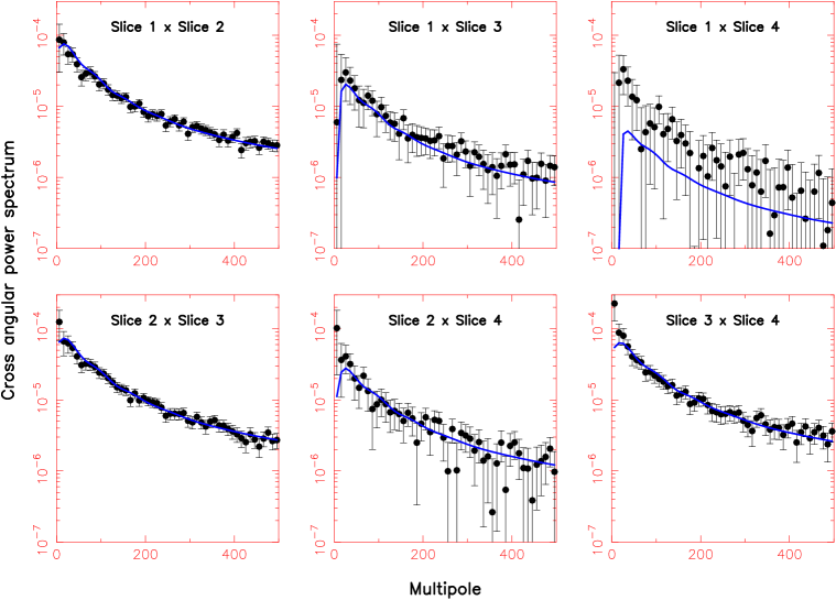
Figure 12: The cross angular power spectra measured between all combinations of the four photometric redshift slices. The plotted models are not fitted to the data points, but are calculated using equation 22 assuming the best-fitting cosmological parameters from the analysis of the auto power spectra.

Using this form of covariance matrix, we re-fitted the cosmological models as before. We marginalized over a separate linear bias parameter for each redshift slice ($b_{1}\rightarrow b_{4}$), thus we are fitting seven parameters ($\Omega_{\rm m}$, $f_{\rm b}$, $\sigma_{8}$, $b_{1}\rightarrow b_{4}$). The probability contours for the matter and baryon densities are displayed in Figure 11. The resulting 1-$\sigma$ measurements of the parameters are $\Omega_{\rm m}=0.26\pm 0.031$ and $f_{\rm b}=0.16\pm 0.036$ (for fixed values of $H_{0}=75$ km s^-1 Mpc^-1 and $n_{\rm scalar}=1$, marginalizing over $\sigma_{8}$ and the four bias parameters). This constitutes a significant detection of the influence of baryons on the clustering pattern of galaxies. The dashed contours in Figure 11 illustrate the effect of reducing the value of $H_{0}$ to 70 km s^-1 Mpc^-1. The resulting shift is exactly as expected given that the clustering pattern is sensitive to the combination $\Omega_{\rm m}H_{0}$. We therefore express our result as $\Omega_{\rm m}h=0.195\pm 0.023$ [where $h=H_{0}/(100$ km s^-1 Mpc^-1)]. The dotted contours in Figure 11 are obtained if $H_{0}=75$ km s^-1 Mpc^-1 but the value of $n_{\rm scalar}$ is reduced to $0.95$. In this case we obtain the marginalized error $\Omega_{\rm m}h=0.21\pm 0.023$.

These parameter measurements agree with the latest analysis of the Cosmic Microwave Background radiation (the 3-year results of the Wilkinson Microwave Anisotropy Probe, see Spergel et al. 2006). The measurements from the CMB data alone are $\Omega_{\rm m}h\approx 0.17\pm 0.03$ and $\Omega_{\rm b}/\Omega_{\rm m}\approx 0.18\pm 0.01$. Our results are also in concord with those derived from the latest spectroscopic redshift surveys. For example, Cole et al. (2005) report $\Omega_{\rm m}h=0.17\pm 0.02$ and $\Omega_{\rm b}/\Omega_{\rm m}=0.19\pm 0.05$ from an analysis of the final 2dF Galaxy Redshift Survey, fixing the Hubble parameter $h$ and scalar index of primordial fluctuations $n_{\rm scalar}$ in a manner similar to our analysis. There is tension at the 1-$\sigma$ level between the different best-fitting values for $\Omega_{\rm m}$, but we ascribe no statistical significance to this. Our parameter constraints are also consistent with the combined analysis of the CMB data and power spectrum of the spectroscopic sample of SDSS LRGs by Huetsi (2006b).

3.4.3 Cross power spectra

Equation 22 can be used to evaluate the cross angular power spectrum between different redshift slices $i$ and $j$ for a given cosmological model. The cross power spectrum can also be measured from the data; this is a useful cross-check on the consistency of our analysis (i.e. the best-fitting cosmological parameters and the redshift distributions within each photo-$z$ slice). The estimator is:

$$C^{i,j}_{\ell}=\frac{1}{2\ell+1}\sum_{m=-\ell}^{\ell}(A^{i}_{\ell,m})^{*}A^{j}_{\ell,m}$$ (23)

where $A^{i}_{\ell,m}$ and $A^{j}_{\ell,m}$ are the spherical harmonic coefficients estimated in redshift slices $i$ and $j$, corrected for partial sky effects as described in Section 3.1. By analogy with equation 13, the variance in this estimator is:

$$\sigma^{2}(C^{i,j}_{\ell})=\frac{2}{f_{\rm sky}(2\ell+1)}\left(C^{i}_{\ell}+\frac{\Delta\Omega}{N_{i}}\right)\left(C^{j}_{\ell}+\frac{\Delta\Omega}{N_{j}}\right)$$ (24)

where $C^{i}_{\ell}$ and $C^{j}_{\ell}$ are the auto angular power spectra in the two redshift slices and $N_{i}$ and $N_{j}$ are the numbers of galaxies analyzed.

Figure 12 plots the measured cross power spectra for the six possible combinations of four redshift slices, together with the model predictions for the best-fitting cosmological parameters from the combined analysis of the auto power spectra of all the redshift slices. Although the cross power spectra have not been used in the cosmological fitting, the agreement is generally excellent. The only combination of redshift slices which performs poorly is 1 and 4, the most separated pair. In this case, the cross-correlation amplitude is generated by the furthest wings of the redshift probability distribution in each slice. In this regime the Gaussian model falls off too quickly, hence the model prediction lies below the cross power spectrum data points.

3.5 Searching for baryon oscillations

We used the angular power spectrum measurements to look for “model-independent” evidence of baryon oscillations in the clustering pattern. We divided out the overall shape of the power spectrum in each case via a smooth polynomial fit, and searched for significant enhancements or reductions in power at the expected scales. The baryon oscillations encode a preferred spatial scale (fixed in co-moving co-ordinates) as an approximately sinusoidal modulation of power in Fourier space. Therefore, given data with a sufficiently high signal-to-noise ratio, we should observe the corresponding preferred angular scales moving to larger values of $\ell$ with increasing redshift, which would constitute an excellent “model-independent” test for the existence of baryon oscillations. Unfortunately, the current data does not possess a sufficiently high signal-to-noise ratio to permit this test. We therefore combined the angular power spectrum measurements in the different redshift slices, scaling a measurement at redshift $z$ along the $x$-axis by a factor proportional to $1/x(z)$ in order to match equivalent spatial scales projected from different redshifts. One binning of the data is plotted in Figure 13, together with a model prediction. We find visual suggestions of baryon oscillations, but the statistical significance is less than 3-$\sigma$. We have not taken into account covariances between redshift slices when constructing Figure 13.

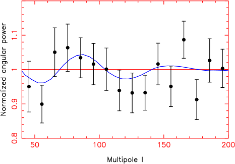
Figure 13: Combination of the angular power spectrum measurements. The data is first divided by a smooth polynomial fit and then scaled along the $x$-axis in order to match equivalent spatial scales projected from different redshifts. The aim is to detect “model-independent” evidence for baryon oscillations in the clustering pattern. The solid sinusoidal line is a model of the result.

4 Tests for systematic photometric errors

In this Section we perform an extensive series of tests for potential systematic photometric errors that may affect our clustering results. Unfortunately, any small photometric errors will be amplified for a sample of Luminous Red Galaxies because these objects are selected from a very steep part of the galaxy luminosity function, where a relatively small shift in the magnitude completeness threshold (e.g., $\Delta m=0.05$) will produce a much larger (10s of per cent) change in the galaxy surface density. In order to search for such effects, we compared the angular power spectrum measured for the “default” sample (defined in Section 2) with that obtained by restricting or extending the galaxy selection in the following ways:

• Exclusion of areas of high dust extinction.

• Exclusion of areas of poor astronomical seeing.

• Exclusion of areas in the vicinity of very bright objects.

• Exclusion of areas lying in the overlap regions between survey stripes.

• Exclusion of areas of low Galactic latitude.

• Separate analysis of the two largest disconnected survey regions in Figure 1.

• Variations in the star-galaxy separation criteria.

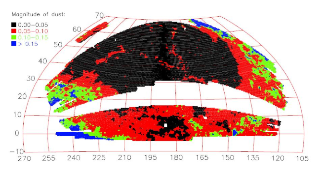
Figure 14: Variation in dust extinction across the DR4 NGP region.

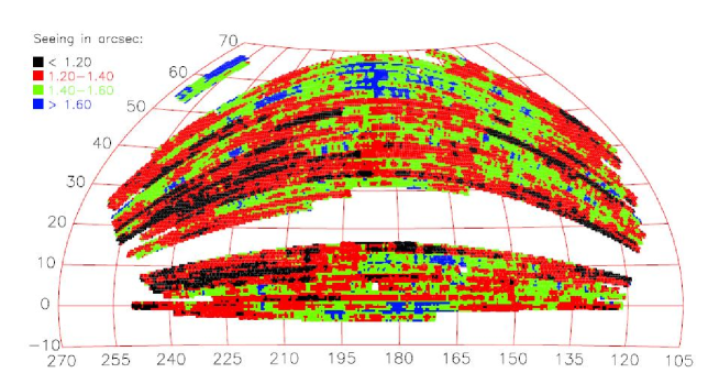
Figure 15: Variation in astronomical seeing across the DR4 NGP region.

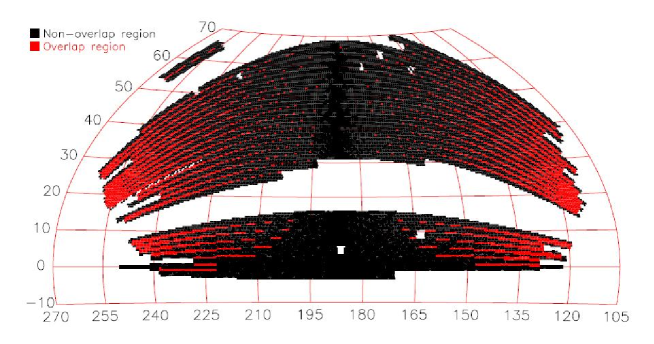
Figure 16: Location of overlap regions between SDSS stripes in the DR4 NGP region.

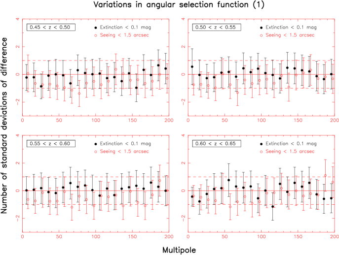
Figure 17: The dependence of the angular power spectrum measurement in 4 redshift slices on varying dust extinction and astronomical seeing. Results from the default catalogue are compared to an analysis restricting the regions analyzed to (1) a maximum dust extinction of $0.1$ mag (see Figure 14), or (2) a maximum seeing of $1.5$ arcsec (see Figure 15). The $x$-axis is multipole $\ell$ and the $y$-axis displays the number of standard deviations of the new measurement from the default result (with $\pm 1\sigma$ marked as horizontal dashed lines).

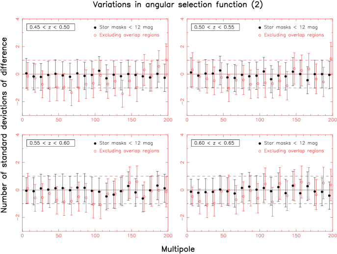
Figure 18: The dependence of the angular power spectrum measurement in 4 redshift slices on the presence of bright objects and stripe overlap regions. Results from the default catalogue are compared to (1) an analysis placing circular masks of radius 1 arcmin around all objects with $i$-band magnitudes brighter than 12, and (2) an analysis excluding overlap regions between stripes (see Figure 16). The results are displayed in the same manner as Figure 17.

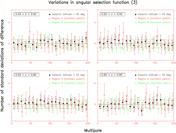
Figure 19: The dependence of the angular power spectrum measurement in 4 redshift slices on Galactic latitude and disconnected region. Results from the default catalogue are compared to (1) an analysis excluding regions below Galactic latitude $45^{\circ}$, and (2,3) a separate analysis of each of the two largest disconnected regions in the survey window function (see Figure 1). The results are displayed in the same manner as Figure 17.

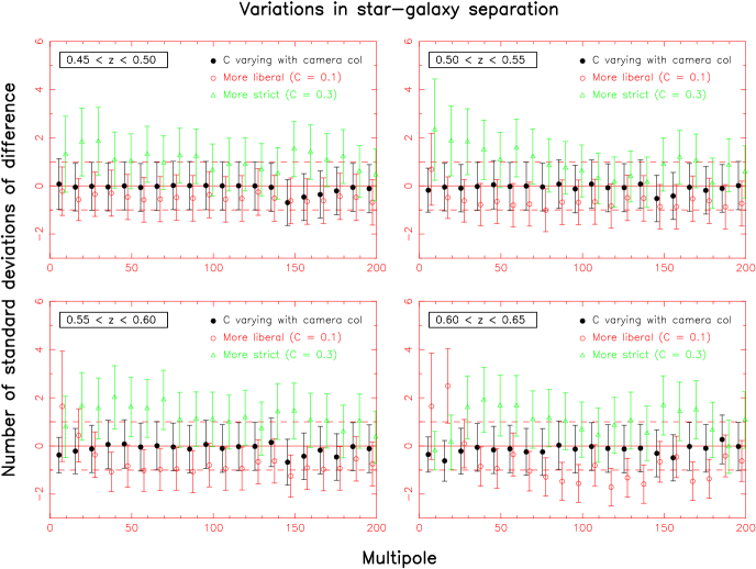
Figure 20: The dependence of the angular power spectrum measurement in 4 redshift slices on the star-galaxy separation criteria. Results from the default catalogue are compared to analyses changing the value of the co-efficient $C$ in equation 25. The results are displayed in the same manner as Figure 17.

4.1 Dust extinction

Figure 14 displays the distribution of dust extinction across the SDSS NGP (obtained from the public database). Variations in dust extinction may imprint systematic changes in galaxy density on the sky near the magnitude limit of the survey, or if there are systematic errors in the extinction map. In this latter case, dust extinction may affect photometric redshift estimates by reddening galaxy colours. We repeated the angular power spectrum measurement excluding regions with high dust extinction ($>0.1$ mag; $14\%$ of the survey area). The results in each of the four redshift slices are shown by the solid circles in Figure 17. These data points illustrate the number of standard deviations by which the angular power spectrum changes from its default value given the variation in the selection criteria. Restricting the analyzed area to regions of low dust extinction produces no significant change in the power spectrum measurement.

4.2 Astronomical seeing

Figure 15 displays the distribution of seeing across the SDSS NGP (obtained from the public database). Poor seeing affects the reliability of the galaxy photometry and the efficacy of the star-galaxy separation. We repeated the angular power spectrum measurement excluding regions with poor seeing ($>1.5$ arcsec; $15\%$ of the survey area). The result is shown by the open circles in Figure 17. Again, any change in the value of the power spectrum is less than the statistical error in the measurement.

4.3 Incompleteness near bright objects

In the immediate vicinity of bright stars or galaxies, the depth (completeness) of the SDSS imaging survey decreases owing to the difficulty in distinguishing close neighbours to these bright objects against the enhanced background. The result is a spurious reduction in the number of very close galaxy pairs (with separations $\theta<0.02^{\circ}$) at faint magnitude thresholds. This effect is negligible for our analysis owing to the large angular scales we are considering (multipoles $\ell\leq 500$ of the angular power spectrum) and to our exclusion of bright ($i_{\rm deV}<17.5$) and faint ($i_{\rm deV}>19.8$) objects. In order to verify this fact, we repeated the angular power spectrum measurement amending the angular selection function by placing a series of circular masks of radius $1^{\prime}$ around very bright SDSS imaging objects with magnitudes $i<12$ (removing $1.4\%$ of the survey area). The result is shown by the solid circles in Figure 18, which differ from the default measurement by much less than the statistical error.

4.4 Stripe overlap regions

The SDSS is performed in scans which result in long data stripes of width $2.5^{\circ}$ spanning the sky. These stripes overlap towards the edges of the surveyed region, as displayed in Figure 16, causing an increase in the effective depth of the survey in these areas of overlap (or equivalently, an increase in the completeness at a fixed magnitude threshold near the survey limit). We repeated the angular power spectrum measurement excluding these overlap regions ($18\%$ of the survey area). The resulting deviation is shown by the open circles in Figure 18. Any differences are small, and we conclude that our faint magnitude threshold of $19.8$ is sufficiently bright that differential completeness effects are unimportant in our analysis.

4.5 Galactic latitude

The residual stellar contamination in our photometric database may be a function of Galactic latitude, potentially imprinting large-scale systematic density fluctuations. Lines of constant Galactic latitude are overlaid on the survey window function in Figure 1. We repeated the angular power spectrum measurement excluding areas with Galactic latitudes below $45^{\circ}$ ($30\%$ of the survey area). The resulting deviation is shown by the solid circles in Figure 19. Again, the differences can be largely accounted for by random statistical error, and we conclude that any sky variation of stellar contamination has a negligible effect on the clustering measurements.

4.6 Analysis of disconnected regions

The survey window function (Figure 1) is mainly comprised of two large disconnected regions. These northern and southern regions, which we will call A and B, comprise $32\%$ and $67\%$ of the total survey area, respectively. The lack of overlap between these regions implies that relative photometric calibration is challenging. It is plausible that some systematic calibration difference between these two regions could imprint apparent large-scale fluctuations in power. We repeated the angular power spectrum measurement for each region separately. The resulting deviations are shown by the open circles and triangles in Figure 19, which reveal no systematic difference in results from the joint analysis of the combination of regions. We conclude that the accuracy of the relative photometric calibration between these two regions is acceptable.

4.7 Star-galaxy separation

The unavoidable presence of a small fraction $f$ of stars in our analyzed catalogue affects the clustering measurement. The addition of a distribution of uncorrelated stars to our clustered galaxies reduces the overall amplitude of the power spectrum. In equation 18, the effect is that the redshift probability distribution $p(z)$ is now normalized to $(1-f)$. To first order, the clustering amplitude is reduced by a factor $(1-f)^{2}$, which may be conveniently absorbed into the constant galaxy bias factor fitted to the data in equation 18.

There are also second order effects. Firstly, problems would arise at low Galactic latitudes owing to the varying stellar density with position. This is not important for the surveyed SDSS regions, as demonstrated above. Secondly, the optical quality of the SDSS camera varies a little with camera column (i.e., perpendicular to the stripe direction) across its $2.5^{\circ}$ diameter. This affects our ability to separate stars and galaxies as a function of SDSS $\nu$-coordinate (i.e., across stripes). Near the edges of the camera, the point-spread function is a little broader, and thus faint compact galaxies will be preferentially mistaken for stars, inducing a fluctuating galaxy surface density with minima at the edges of stripes. The angular scale of the resulting fluctuations will be similar to the width of the stripes, $2.5^{\circ}$. Unfortunately, this is comparable to the preferred angular scale of the baryon oscillations ($\approx 5^{\circ}$ at $z=0.5$).

In Figure 21 we illustrate this effect by plotting the average overdensity of the LRG catalogue as a function of pixel position across the field-of-view of the SDSS camera. We bin galaxies as a function of the quantity $x=3000\times(n_{\rm cam}-1)+n_{\rm col}$, where $n_{\rm cam}$ is the SDSS camera column containing the object (an integer between 1 and 6), $n_{\rm col}$ is the pixel position of the galaxy centroid in that column (a decimal up to 2048), and 3000 is an arbitrary offset to separate the camera columns clearly in the Figure. The solid points represent the average galaxy overdensity using the star-galaxy separation criteria described by Collister et al. (2006),

$$i_{\rm psf}-i_{\rm model}\geq C\times(21-i_{\rm deV})$$

$$\theta_{i,{\rm deV}}\geq 0.2^{\prime\prime}$$ (25)

where the coefficient $C=0.2$. In this analysis we do not include any additional neural network star-galaxy separation using ANNz (see Section 2). For the reasons discussed above, the resulting LRG overdensity peaks in column 3 and has minima at the camera edges (columns 1 and 6). In order to correct for this systematic imprint, we tried varying the coefficient $C$ in equation 25 to trace the quality of the star-galaxy separation, such that $C$ assumed different values $(0.1,0.2,0.25,0.2,0.2,0.16)$ in the six camera columns. These modified values of $C$ are chosen to ensure that the average galaxy overdensity is constant across the camera field (the open circles in Figure 21).

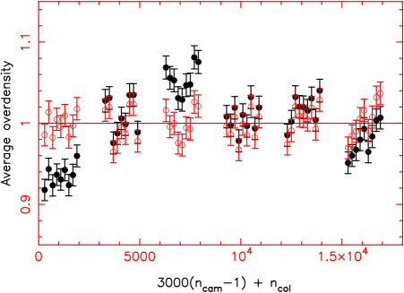
Figure 21: The average overdensity of LRGs as a function of pixel position across the SDSS camera (perpendicular to the direction of the camera columns). This position is quantified by the value of $3000\times(n_{\rm cam}-1)+n_{\rm col}$, where $n_{\rm cam}$ is the camera column, $n_{\rm col}$ is the pixel position of the galaxy centroid in that column, and 3000 is an arbitrary offset to separate the camera columns clearly in the Figure. Owing to the varying optical quality of the camera across the field-of-view, if constant star-galaxy separation criteria are applied then the resulting overdensity profile will exhibit a peak at the centre of the field with minima at the edges (as shown by the solid circles). In order to correct for this effect, we varied the aggressiveness of the star-galaxy separation as a function of camera column as described in the text, removing the systematic density variation (as shown by the open circles).

We then repeated the angular power spectrum measurement comparing our catalogue with default star-galaxy separation ($C=0.2$) to the model where $C$ varies with camera column. We also considered alternative constant values $C=0.1$ and $C=0.3$. The results are displayed in Figure 20. Our first conclusion is that the adoption of the camera column-dependent star-galaxy separation is of negligible benefit. The imprint of the varying overdensity in Figure 21 in fact has no measurable effect on the power spectrum. We therefore retain our default criteria of a constant coefficient $C=0.2$. The effect of changing this value is in reasonable accord with our model of a constant factor in power, which may be safely absorbed into the fitted galaxy bias factor. The possible exception to this conclusion is the lowest multipole bands in the furthest redshift slice $0.6<z<0.65$ (which is expected to contain the most significant stellar contamination). In this case, more liberal star-galaxy separation actually increases the observed power on the largest scales. In fact, the lowest multipole band for this redshift slice is observed to possess marginally significant excess power in Figure 10, thus this one data point may be influenced by stellar contamination.

5 Measurement of the spatial power spectrum

In this Section we determine the spatial galaxy power spectrum by a direct three-dimensional Fourier transform of the gridded photo-$z$ catalogue. We believe that this is a novel technique which has not been previously applied to galaxy data, although Seo & Eisenstein (2003) and Blake & Bridle (2005) give theoretical discussions.

5.1 Method

The photo-$z$ error distribution produces a convolution of the underlying density field in the radial direction, and hence (in the first approximation) a multiplicative radial damping of the measured three-dimensional power in Fourier space. In principle this damping factor can be calculated using the known photo-$z$ error properties and then divided out, restoring the underlying unconvolved power spectrum. We must implement a flat-sky approximation such that the photo-$z$ smearing only occurs along one axis.

For example, in the ideal case that the radial co-moving co-ordinate $x$ of each galaxy is smeared by an amount $\delta x$ sampled from a Gaussian distribution

$$f(\delta x)\propto\exp{\left[-\frac{1}{2}\left(\frac{\delta x}{\sigma_{x}}\right)^{2}\right]}$$ (26)

then the resulting power spectrum signal will be damped in the radial direction in accordance with:

$$P(k_{x},k_{y},k_{z})\rightarrow P(k_{x},k_{y},k_{z})\times\exp{[-(k_{x}\,\sigma_{x})^{2}]}$$ (27)

Thus Fourier modes with high values of $|k_{x}|\gg 1/\sigma_{x}$ contribute only noise to the measurement. However, if we only retain power-spectrum modes with $|k_{x}|<k_{x,{\rm max}}\sim 1/\sigma_{x}$, then we can deconvolve the measured 3D power spectrum by dividing by the function $\exp{[-(k_{x}\,\sigma_{x})^{2}]}$ prior to combining the Fourier modes in bins of fixed $k=\sqrt{k_{x}^{2}+k_{y}^{2}+k_{z}^{2}}$ (where $k_{x}<k_{x,{\rm max}}$). In practice the photo-$z$ error distribution is not a constant Gaussian function, and we calculated the deconvolution function for our sample using Monte Carlo simulations rather than an analytic approximation, as described below.

We initially analyzed the galaxies in photometric redshift slices of width $\Delta z=0.05$, as for the angular power spectrum measurement. We implemented the flat-sky approximation by dividing the survey area into patches of width $20\times 20$ deg. These patches have sufficient area to contain a reasonable number of large-scale power spectrum modes with $k<0.2\,h$ Mpc^-1, and yet are small enough that the photo-$z$ smearing may be considered to act along one axis of a survey cuboid (which we take as the $x$-axis). We only analyzed patches for which the survey angular selection function covered over $50\%$ of the area of the patch. The equations mapping the galaxy right ascensions and declinations $(\alpha,\delta)$ onto spatial positions $(X,Y,Z)$ in the cuboid are

$$X = \frac{dx}{dz}(z_{0})\times(z-z_{0})$$

$$Y = x(z_{0})\times(\alpha-\alpha_{0})\cos{\delta_{0}}$$

$$Z = x(z_{0})\times(\delta-\delta_{0})$$ (28)

where $(\alpha_{0},\delta_{0})$ are the central angular co-ordinates of each patch, $z$ is the galaxy redshift, $z_{0}$ is the central redshift of each slice, and $x(z)$ is the co-moving radial distance of the survey redshift. Thus we must assume values for the cosmological parameters to construct this mapping, as discussed below.

We then measured the 3D power spectrum of galaxies in each cuboid in Fourier bins of width $\Delta k=0.01\,h$ Mpc^-1, correcting for survey window function effects and assuming a radial selection function which we directly fitted to the survey data. We only included a Fourier mode $(k_{x},k_{y},k_{z})$ in the analysis if the radial wavescale $|k_{x}|<k_{x,{\rm max}}=1.5/\sigma_{x}$, where $\sigma_{x}$ is the standard deviation of the photo-$z$ errors within the slice in co-moving co-ordinates. For redshift slices of thickness $\Delta z=0.05$ this restricts us to modes with $k_{x}=0$, because the spacing of the modes in radial $k$-space is $\Delta k_{x}=2\pi/L_{x}>k_{x,{\rm max}}$, where $L_{x}$ is the width of the slice in co-moving co-ordinates (we also calculate the spatial power spectrum for a wider redshift slice with $\Delta z=0.15$). The final power spectrum was determined by averaging the measurements in the separate patches. The error in the power spectrum was taken to be the standard deviation of the measurements in the patches.

The calculation of the spatial power spectrum $P(k)$ in this manner depends upon the choice of cosmological parameters (which specifies the cosmological distances $x(z)$ in equation 28). Therefore, the determination of best-fitting cosmological parameters using this method must proceed in a more complex fashion than the angular power spectrum fits in Section 3. In a measurement of $P(k)$, both the data and the model depend on the trial cosmological parameters. In contrast, the measured angular power spectrum does not depend on the cosmological parameters and may be left fixed during the model-fitting process.

However, there is an important advantage in performing a direct measurement of $P(k)$ from a photo-$z$ catalogue: we avoid unnecessary radial binning of the data. The projection of $P(k)$ to the angular power spectrum $C_{\ell}$ (equation 18) corresponds to a convolution of $P(k)$ in Fourier space in which the contrast of any features (such as the baryon oscillations) will be reduced. But direct manipulation of the 3D power spectrum involves only a multiplicative damping of power (equation 27) which does not diminish the contrast of features. Hence the direct power spectrum technique presented in this Section may yield the most significant detection of baryon oscillations. In this initial study we do not in fact fit cosmological parameters to the $P(k)$ measurements, but instead assume the best-fitting set of parameters from the angular power spectrum analysis (Table 2) in order to demonstrate the consistency of the results and to search for the existence of baryon oscillations.

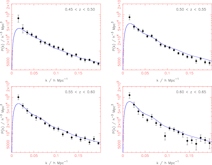
Figure 22: The spatial power spectrum of the photo-$z$ catalogue in each of four redshift slices of width $\Delta z=0.05$, measured using direct Fourier techniques in a series of $20\times 20$ deg patches. There is no data point in the first bin (at $k=0.005\,h$ Mpc^-1) because this bin contains no Fourier modes in the patches. The solid lines are not a fit to this data, but are the model power spectra corresponding to the best-fitting cosmological parameters $(\Omega_{\rm m},f_{\rm b},\sigma_{8},b)$ for the angular power spectrum analysis in each redshift slice. The good agreement between the data and model validates our analysis techniques.

The spatial power spectrum measured by this direct Fourier calculation must be carefully normalized when the condition $\sigma_{x}\ll L_{x}$ is not satisfied, i.e., when the photo-$z$ error is comparable to the width of the survey slice (which is the case here). For a spectroscopic survey of volume $V$, the dimensionless power spectrum of the Fourier amplitudes, $|\delta_{k}|^{2}$, must be multiplied by $V$ in order to obtain a measured quantity (e.g. with units of $h^{-3}$ Mpc³) which is independent of the volume of the survey and may be compared with theoretical predictions. Suppose this spectroscopic survey is now convolved with a photo-$z$ error function, and a radial slice of the resulting photo-$z$ catalogue is analyzed, with volume $V_{\rm slice}$. The correct normalization factor for comparison of the measured power spectrum with theory is not in fact $V_{\rm slice}$, because the galaxy distribution within the slice has been smoothed over a wider volume owing to the scattering of objects into the slice by the photo-$z$ error distribution. In the ideal case of a “top-hat” radial selection function for the photo-$z$ slice (of width $L_{x}$) and the Gaussian photo-z error function of equation 26, the multiplicative normalization correction is given by

$$N=\frac{1}{2\pi}\int_{-\infty}^{\infty}du\,\exp{\left[-\left(\frac{u}{L_{x}/\sigma_{x}}\right)^{2}\right]}\left[\frac{\sin{(u/2)}}{(u/2)}\right]^{2}$$ (29)

such that the effective normalization volume for the power spectrum measurement is $V_{\rm slice}/N$. Equation 29 has the limits $N\rightarrow 1$ for $\sigma_{x}\ll L_{x}$ (i.e., a spectroscopic survey) and $N\rightarrow L_{x}/(2\sqrt{\pi}\sigma_{x})$ for $L_{x}\ll\sigma_{x}$.

Moreover, the smoothing of the density distribution from outside the photo-$z$ slice affects the shot noise correction term $P_{\rm shot}$ subtracted from the raw power spectrum measurement, $|\delta_{k}|^{2}$. The shot noise correction is not simply given by the volume density $n$ of analyzed galaxies within the slice, $P_{\rm shot}=1/n$. Thus the measured power spectrum $P_{\rm meas}$ must be adjusted by both additive (shot noise) and multiplicative (normalization) corrections in order to achieve a reliable estimate of the underlying power spectrum $P_{\rm true}$:

$$P_{\rm true}(k)=A(k)\,P_{\rm meas}(k)+B(k)\,P_{\rm shot}$$ (30)

where $A(k)$ and $B(k)$ are roughly constant with $k=\sqrt{k_{x}^{2}+k_{y}^{2}+k_{z}^{2}}$, although change rapidly with $k_{x}$ ($\leq k_{x,{\rm max}}\ll k)$ owing to the exponential damping factor in equation 27.

We determined the two correction functions $A(k)$ and $B(k)$ in equation 30 using Monte Carlo realizations. We first generated clustered distributions of galaxies in a three-dimensional survey cone, using a model spatial power spectrum corresponding to the best-fitting cosmological parameters. These Gaussian power-spectrum realizations were created using the method described in Glazebrook & Blake (2005). The radial selection function before the application of photometric redshift errors was fixed by the spectroscopic redshift distribution of the 2SLAQ training set (our best estimate of the unconvolved redshift distribution). The SDSS angular selection function of Figure 1 was then imposed. We then applied a photometric redshift convolution function, again determined using the training set, such that a different photo-$z$ error distribution is implemented at each spectroscopic redshift, to ensure maximum consistency with the statistics of the real catalogue. The appropriate photo-$z$ slices were then isolated and the spatial power spectra were measured with the same methods as applied to the real data. In order to complete the calculation, a second set of Monte Carlo realizations was generated using an identical method, except that the original spectroscopic catalogue was unclustered (i.e., $P_{\rm true}=0$ in equation 30) and thus the measured power spectrum purely probes shot noise effects. The two measured power spectra, of the clustered and unclustered simulations, in conjunction with the known input power spectrum, allow us to deduce the functions $A(k)$ and $B(k)$ in equation 30. These correction factors are then applied to our power spectrum measurements from the real data.

5.2 Results

We display our spatial power spectrum measurements in the four redshift slices in Figure 22, together with the models corresponding to the best-fitting cosmological parameters from the angular power spectrum analysis (Table 2). The agreement is good, validating our analysis techniques. There is evidence of excess power in the largest-scale bin, possibly due to the failure of the small-angle approximation of equation 28 on these scales. We note that redshift-space distortions do not affect the power spectrum models plotted in Figure 22 because we are only analyzing power spectrum modes with $k_{x}=0$. The power spectrum boost due to large-scale coherent infall depends on the angle to the line-of-sight $\theta$ of a given Fourier mode as $(1+\beta\cos^{2}{\theta})$, thus modes with $k_{x}\approx 0$ (i.e. $\theta\approx 90^{\circ}$) contain little imprint of redshift-space effects.

In Figure 23 we plot the results of analyzing a wider redshift slice of the survey, $0.475<z<0.625$, such that Fourier modes with $k_{x}\neq 0$ are being utilized. Again, agreement with the model spatial power spectrum is very good. The shape of our recovered power spectra also agree well with the measurement from the spectroscopic sample of SDSS LRGs at lower redshift by Huetsi (2006a).

Unfortunately the current size of the survey is not sufficient to yield convincing “model-independent” evidence for baryon oscillations. However, a modest expansion of the survey volume (e.g. the final SDSS Data Release) would clearly create the potential to produce such a detection (as modelled by Blake & Bridle 2005).

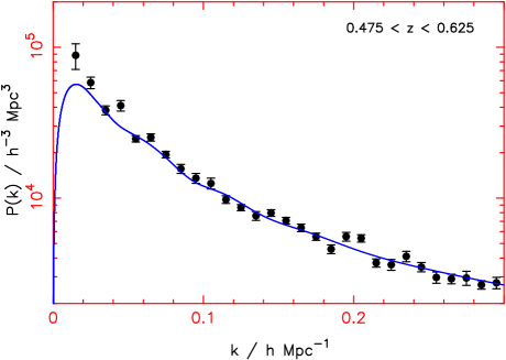
Figure 23: The spatial power spectrum of the photo-$z$ catalogue in a wide redshift slice $\Delta z=0.15$ such that Fourier modes with $k_{x}\neq 0$ are utilized in the analysis. The agreement is good with the model power spectrum corresponding to the best-fitting cosmological parameters for the angular clustering measurements (the solid line).

6 Conclusions

We have quantified the patterns of large-scale structure in a photometric-redshift catalogue of intermediate-redshift ($0.4<z<0.7$) Luminous Red Galaxies from the SDSS 4th Data Release. This catalogue, which we have named MegaZ-LRG, contains $>10^{6}$ photometric redshifts derived with ANNz, an Artificial Neural Network code (Collister et al. 2006). In this study we analyze a “conservative” version of the catalogue, which includes $6\times 10^{5}$ objects over $5{,}914$ deg². The main conclusions of our study are:

• We measured angular power spectra in a series of photo-$z$ slices of width $\Delta z=0.05$ from $z=0.45$ to $z=0.65$. The errors in the $C_{\ell}$ spectra were tested with Monte Carlo realizations and with a “bootstrap” analysis in sub-fields. A simple Gaussian approximation was determined to be an accurate approximation to the error in $C_{\ell}$ over the scales of interest.

• The angular power spectra are well-fitted by model spatial power spectra with consistent cosmological parameters $\Omega_{\rm m}\approx 0.27$, $f_{\rm b}\approx 0.17$, $H_{0}=75$ km s^-1 Mpc^-1 and $n_{\rm scalar}=1$ over the series of redshift slices.

• Combining the results for the different redshift slices with appropriate covariances results in a measurement of $\Omega_{\rm m}h=0.195\pm 0.023$ and $\Omega_{\rm b}/\Omega_{\rm m}=0.16\pm 0.036$ (for fixed values of $H_{0}$ and $n_{\rm scalar}$, marginalizing over $\sigma_{8}$ and $b$). These measurements agree with the latest analysis of the Cosmic Microwave Background radiation (the 3-year results of the Wilkinson Microwave Anisotropy Probe, see Spergel et al. 2006). The measurements from the CMB data alone are $\Omega_{\rm m}h=0.17\pm 0.03$ and $\Omega_{\rm b}/\Omega_{\rm m}=0.18\pm 0.01$.

• These results agree very well with a parallel investigation of a similar dataset carried out by Padmanabhan et al. (2006) using a different photometric-redshift estimation method and power spectrum analysis procedure. Padmananhan et al. quote cosmological parameter fits $\Omega_{\rm m}h=0.21\pm 0.021$ and $\Omega_{\rm b}/\Omega_{\rm m}=0.18\pm 0.04$, in both cases within 1-$\sigma$ of our results.

• We detect visual suggestions of baryon oscillations with a statistical significance of less than 3-$\sigma$.

• We performed a direct re-construction of the spatial power spectrum using a Fourier analysis which only retains large-scale radial components. We demonstrated that this method produces results which are consistent with the best-fitting model for the angular power spectrum analysis.

• We searched for evidence of systematic photometric errors in the catalogue using a variety of tests, and were unable to identify any significant effects.

• We measure a hint of excess power relative to the best-fitting cosmological model on the largest scales (the lowest multipole bands in the four redshift slices in Figure 10). If confirmed, this excess power has a range of possible causes: (1) residual systematic errors; (2) cosmic variance; (3) large-scale galaxy biasing mechanisms; (4) new early-Universe physics.

The cosmological parameter measurements we obtain from the large-scale clustering of this photometric redshift catalogue have a similar precision to those derived from the latest spectroscopic redshift surveys, despite the weaker redshift information. For example, Cole et al. (2005) report $\Omega_{\rm m}h=0.17\pm 0.02$ and $\Omega_{\rm b}/\Omega_{\rm m}=0.19\pm 0.05$ from an analysis of the final 2dF Galaxy Redshift Survey, fixing the Hubble parameter $h$ and scalar index of primordial fluctuations $n_{\rm scalar}$ in a manner similar to our analysis. We therefore conclude that photometric redshift surveys have become competitive with spectroscopic surveys for the measurement of cosmological parameters using the large-scale clustering pattern in the simple “vanilla” model.

References

- [1] Amendola L., Quercellini C., Giallongo E., 2005, MNRAS, 357, 429
- [2] Baugh C.M., Efstathiou G., 1993, MNRAS, 265, 145
- [3] Blake C.A., Glazebrook K., 2003, ApJ, 594, 665
- [4] Blake C.A., Ferreira P.G., Borrill J., 2004, MNRAS, 351, 923
- [5] Blake C.A., Bridle S.L., 2005, MNRAS, 363, 1329
- [6] Budavari T. et al., 2003, ApJ, 595, 59
- [7] Cannon R. et al., 2006, MNRAS submitted (astro-ph/0607631)
- [8] Chiang L.-Y., Coles P., 2000, MNRAS, 311, 809
- [9] Coil A.L., Newman J.A., Kaiser N., Davis M., Ma C.-P., Kocevski D.D., Koo D.C., 2004, ApJ, 617, 765
- [10] Cole S. et al., 2005, MNRAS, 362, 505
- [11] Colless M. et al., 2001, MNRAS, 328, 1039
- [12] Collister A., Lahav O., 2004, PASP, 116, 345
- [13] Collister A. et al., 2006, MNRAS submitted (astro-ph/0607630)
- [14] Davis M. et al., 2003, Proc. SPIE, 4834, 161
- [15] Deligny O. et al., 2004, JCAP, 10, 8
- [16] Dodelson S., 2003, Modern Cosmology, Academic Press Inc., U.S.
- [17] Dolney D., Jain B., Takada M., 2004, MNRAS, 352, 1019
- [18] Efstathiou G., Sutherland W.J., Maddox S.J., 1990, Nature, 348, 705
- [19] Efstathiou G., Moody S., 2001, MNRAS, 325, 1603
- [20] Efstathiou G. et al., 2002, MNRAS, 330, L29
- [21] Efstathiou G., 2004, MNRAS, 349, 603
- [22] Eisenstein D.J. et al., 2001, AJ, 122, 2267
- [23] Eisenstein D.J. et al., 2005, ApJ, 633, 560
- [24] Firth A.E., Lahav O., Somerville R.S., 2003, MNRAS, 339, 1195
- [25] Fisher K.B., Scharf C.A., Lahav O., 1994, MNRAS, 266, 219
- [26] Glazebrook K., Blake C.A., 2005, ApJ, 631, 1
- [27] Hauser M.G., Peebles P.J.E., 1973, ApJ, 185, 757
- [28] Hivon E., Gorski K.M., Netterfield C.B., Crill B.P., Prunet S., Hansen F., 2002, ApJ, 567, 2
- [29] Huetsi G., 2006a, A&A, 449, 891
- [30] Huetsi G., 2006b, A&A submitted (astro-ph/0604129)
- [31] Huterer D., Knox L., Nichol R.C., 2001, ApJ, 555, 547
- [32] Lahav O. et al., 2002, MNRAS, 333, 961
- [33] Le Fevre O. et al., 2003, Proc. SPIE, 4834, 173
- [34] Le Fevre O. et al., 2005, A&A, 439, 877
- [35] Lewis A., Challinor A., Lasenby A., 2000, ApJ, 538, 473
- [36] Magliocchetti M. et al., 2000, MNRAS, 314, 546
- [37] Norberg P. et al., 2002, MNRAS, 336, 907
- [38] Ostriker J.P., Steinhardt P.J., 1995, Nature, 377, 600
- [39] Padmanabhan N. et al., 2005, MNRAS, 359, 237
- [40] Padmanabhan N. et al., 2006, MNRAS submitted (astro-ph/0605302)
- [41] Peebles P.J.E., 1973, ApJ, 185, 413
- [42] Percival W.J. et al., 2001, MNRAS, 327, 1297
- [43] Percival W.J. et al., 2002, MNRAS, 337, 1068
- [44] Perlmutter S. et al., 1999, ApJ, 517, 565
- [45] Pope A. et al., 2004, ApJ, 607, 655
- [46] Riess A.G. et al., 1998, AJ, 116, 1009
- [47] Sanchez A.G., Baugh C.M., Percival W.J., Peacock J.A., Padilla N.D., Cole S., Frenk C.S., Norberg P., 2006, MNRAS, 366, 189
- [48] Scharf C., Hoffman Y., Lahav O., Lynden-Bell D., 1992, MNRAS, 256, 229
- [49] Scranton R. et al., 2005, ApJ, 633, 589
- [50] Seljak U., Zaldarriaga M., 1996, ApJ, 469, 437
- [51] Seljak U. et al., 2005, Phys.Rev.D., 71, 103515
- [52] Seo H., Eisenstein D.J., 2003, ApJ, 598, 720
- [53] Smith R.E. et al., 2003, MNRAS, 341, 1311
- [54] Spergel D.N. et al., 2003, ApJS, 148, 175
- [55] Spergel D.N. et al., 2006, ApJ submitted (astro-ph/0603449)
- [56] Tegmark M. et al., 2002, ApJ, 571, 191
- [57] Tegmark M. et al., 2004a, ApJ, 606, 702
- [58] Tegmark M. et al., 2004b, Phys.Rev.D., 69, 103501
- [59] Wandelt B.D., Hivon E., Gorski K.M., 2001, PhRvD, 64, 3003
- [60] Wright E.L., Smoot G.F., Bennett C.L., Lubin P.M., 1994, ApJ, 436, 441
- [61] Wolf C., Meisenheimer K., Rix H.-W., Borch A., Dye S., Kleinheinrich M., 2003, A&A, 401, 73
- [62] York D.G. et al., 2000, AJ, 120, 1579
- [63] Zehavi I. et al., 2005, ApJ, 621, 22
- [64] Zhan H., Knox L., Tyson J.A., Margoniner V., 2006, ApJ, 640, 8