The Far Ultraviolet Spectroscopic Explorer Survey of O VI Emission in the Milky Way

Abstract

We present a survey of O VI $\lambda$1032 emission in the Milky Way using data from the Far Ultraviolet Spectroscopic Explorer (FUSE) satellite. The observations span the period from launch in 1999 to July 2003. Our survey contains 112 sight lines, 23 of which show measurable O VI $\lambda$1032 emission. The O VI $\lambda$1032 emission feature was detected at all latitudes and exhibits intensities of 1900–8600 photons s^-1 cm^-2 sr^-1. Combined with values from the literature, these emission measurements are consistent with the picture derived from recent O VI absorption surveys: high-latitude sight lines probe O VI-emitting gas in a clumpy, thick disk or halo, while low-latitude sight lines sample mixing layers and interfaces in the thin disk of the Galaxy.

1 INTRODUCTION

Hot interstellar gas cooling through temperatures of a few times $10^{5}$ K is most easily studied through observations of the lithium-like ions C IV, Si IV, N V, and O VI. The O VI resonance transitions at 1031.93 and 1037.62 Å provide the primary cooling mechanism for collisionally-ionized gas at temperatures near $3\times 10^{5}$ K, while the corresponding lines of N V ($\lambda\lambda 1238.81,1242.80$), C IV ($\lambda\lambda 1548.19,1550.76$), and Si IV ($\lambda\lambda 1393.76,1402.77$) dominate at cooler temperatures (Sutherland & Dopita, 1993). Extensive studies of interstellar N V, C IV, and Si IV absorption have been performed with the International Ultraviolet Explorer (IUE) (e.g., Sembach & Savage, 1992; Sembach, 1993) and with the GHRS and STIS spectrographs aboard the Hubble Space Telescope (e.g., Spitzer, 1996), but, except for a survey of O VI absorption toward 72 nearby stars conducted with the Copernicus satellite (Jenkins, 1978a, b), large surveys of O VI in the Galactic disk and halo have had to await the launch of FUSE, the Far Ultraviolet Spectroscopic Explorer. Recent O VI absorption-line surveys include Wakker et al. (2003), Savage et al. (2003), Bowen et al. (2006), and Savage & Lehner (2006). Indebetouw & Shull (2004a, b) recently obtained both FUSE and HST observations toward 34 stars and compared the derived ionization ratios of the Li-like absorbers with various theoretical models.

By themselves, absorption lines yield the total column of the absorbing species integrated along the line of sight, but when combined with emission-line data, they can be used to derive the local density of the emitting gas (Shull & Slavin, 1994), providing a powerful diagnostic of the microphysics of cooling in these regions. O VI emission has been observed with FUSE along a handful of sight lines, but more observations are required to investigate the distribution, kinematics, and emission mechanisms of O VI-bearing gas in the Galaxy. We searched the FUSE archive for additional sight lines with O VI emission. From a sample of 112 sight lines, we detect O VI emission in 23. We describe our data sample and reduction techniques in §§ 2 and 3. Section 4 explains the data fitting and presents our results. In § 5, we compare these results with various models and with observations obtained at other wavelengths and discuss our results. We summarize our findings in § 6.

2 OBSERVATIONS

The FUSE instrument consists of four independent optical paths. Two employ LiF-coated gratings and mirrors that are sensitive to the wavelengths between 990 and 1187 Å, and two use SiC coatings that are sensitive to wavelengths between 905 and 1100 Å. Each spectrograph possesses three apertures that simultaneously observe different parts of the sky. The low resolution (LWRS) aperture samples an area of $30\arcsec\times 30\arcsec$. The medium resolution (MDRS) aperture spans $4\arcsec\times 20\arcsec$ and lies about $3\farcm 5$ from the LWRS aperture. The high resolution (HIRS) aperture lies between the MDRS and LWRS apertures (about $1\farcm 8$ from the LWRS aperture) and samples an area $1\farcs 25\times 20\arcsec$ wide. A complete description of FUSE can be found in Moos et al. (2000) and Sahnow et al. (2000).

The data used in our survey consist of LiF1A LWRS spectra from the S405 and Z907 programs (as of 2003 July 25) taken in time-tag mode. The S405 programs represent background observations and observations for alignment of the four optical paths. The Z907 programs contain observations of active galactic nuclei (AGNs) and other extragalactic targets that can be used as background sources for absorption studies. In some cases, these targets were too faint for use as background sources, which resulted in relatively flat continua suited for the search of Galactic O VI emission. In addition to these two programs, we searched the Multimission Archive at Space Telescope (MAST; as of 2003 July 25) for MDRS observations of point sources obtained in time-tag mode, as their LWRS apertures should sample only background radiation. If HIRS time-tag observations exist in addition to the MDRS observations of a target, the corresponding LWRS spectra of both MDRS and HIRS observations were combined into one spectrum. When combining LWRS data from HIRS and MDRS observations obtained at different epochs, we ignored the fact that the LWRS aperture may sample slightly different regions of the sky depending on the aperture and position angle used for the observations. At worst, this simplification decreases the spatial resolution of our data from 30 arcsec (the width of the LWRS aperture) to 7 arcmin (twice the distance between LWRS and MDRS aperture).

The sample was further modified as follows: All extracted LWRS spectra that showed continuum flux were removed from the survey. We also removed sight lines whose O VI emission could be identified as originating in the supernova remnants Vela or the Cygnus Loop, since these structures do not represent the diffuse interstellar medium. Sight lines passing within a few arc minutes of the hot white dwarf KPD 0005+511 exhibit unusually strong O VI emission (up to 25,000 LU). We determined that the emission from this region originates in a high-ionization planetary nebula (HIPN) around the white dwarf (Otte, Dixon, & Sankrit 2004), and therefore removed all observations toward this object from the survey.

Three additional white dwarfs exhibit highly ionized circumstellar environments possibly probed by our survey; Si IV, C IV, and N V have been detected in their IUE and/or STIS spectra (Holberg, Barstow, & Sion 1998; Bannister et al., 2003). One of these stars, the white dwarf WD 0455-282, lies within a few arc minutes of our sight lines P10411 ($l=229\fdg 3$) and S40537 ($l=230\fdg 7$), both of which exhibit O VI emission. Holberg et al. (1998) quote absorption in IUE data at $v_{\rm helio}=16\pm 3$ km s^-1 and suggest that this absorption is circumstellar. The O VI emission of S40537 ($v_{\rm helio}=-7\pm 19$ km s^-1) is less likely to be of circumstellar origin than the emission observed along sight line P10411 ($v_{\rm helio}=+10\pm 12$ km s^-1). The low temperature of WD 0455-282 ($T_{\rm eff}=57,200$ K; Savage & Lehner, 2006), however, makes the photoionization of the circumstellar material to high ionization levels such as O VI difficult. While we cannot rule out the possibility of a HIPN around WD 0455-282, we include P10411 in our sample of diffuse O VI emission. The nearby LWRS spectra of the other two white dwarfs, KPD 1034+001 (S40509, $l=247\fdg 6$) and G191–B2B (S40576, $l=156\fdg 0$), do not show any measurable O VI emission.

Five of our sight lines lie within 5° of the ecliptic plane, where solar O VI emission scattered off interplanetary dust is a concern, but we have found no evidence for such contamination in the data. P12012 ($l=194\fdg 3$) is a science observation with Jupiter in the MDRS aperture. Its LiF1A spectrum shows O VI emission with a heliocentric velocity consistent with zero. Its night-only SiC2A spectrum, however, shows no C III $\lambda$977 emission, which would be bright if the O VI emission were solar. The atmosphere of Jupiter consists primarily of H₂. While there is a possibility that the observed emission comes from H₂ fluorescence excited by solar O VI emission, the absence of other H₂ emission lines and the 3$\farcm$5 separation between the MDRS and the LWRS aperture argue against this possibility. The other four sight lines in the ecliptic plane show no O VI emission.

Sight line P10413 ($l=162\fdg 6$) is a science observation with Capella in the MDRS aperture. The stellar spectrum shows strong O VI emission lines with a possible contamination of the HIRS and LWRS aperture. The measured velocity of the O VI emission line in the LWRS aperture, however, is inconsistent with the radial velocities of either star in this spectroscopic binary during the orbital phase at the time of the FUSE observations (Young et al., 2001).

In a few cases, we combined into a single spectrum sight lines that are separated by less than $0\fdg 1$ to improve the signal-to-noise ratio. Table 1 lists the target IDs (usually the first 6–8 characters of the observation ID) by which we identify the sight lines in this survey and the observations that contribute to each. The original sample contained 225 sight lines, of which 77 were removed because of continuum flux or even absorption features in the LWRS aperture; 16 more sight lines were removed because of SNR or HIPN emission. Another 16 sight lines were combined with nearby sight lines, and four observations turned out not to contain any night time data. The final survey contains 112 sight lines unevenly distributed on the sky (Fig. 1). The apparent clustering of observations in two quadrants can be explained by observational constraints that combine to reduce target availability around the orbital plane, which stretches across the Galactic center.

3 DATA REDUCTION

In several cases, observations of the same target were repeated months or even years apart. Using the CalFUSE pipeline to combine these time-tag observations can yield faulty wavelength and thus velocity information. We developed software in IDL to optimize the extraction of the O VI emission from the LiF1A channel by calibrating each exposure individually in wavelength (using O I airglow lines) and flux before combining them into one spectrum. We used the raw data and applied the first steps of the CalFUSE pipline (version 2.3; initializing the header, computing Doppler corrections). Our IDL program then extracted all photons that were detected in a rectangular area around the expected location of O VI in the LWRS spectrum. This rectangular region was determined from the data set S4054801, a very long background observation.

The LWRS spectrum was collapsed perpendicular to the wavelength dispersion axis to create a one-dimensional spectrum. The S4054801 data yielded the template positions of the five O I airglow lines ($\lambda\lambda$1027.431, 1028.157, 1039.230, 1040.943, and 1041.688) surrounding the O VI $\lambda\lambda$1032,1038 doublet. The strongest of these airglow lines is O I $\lambda$1027. Our IDL program searched for an emission line in each individual exposure in a 160 pixel wide window around the O I $\lambda$1027 template position and fitted its position with a Gaussian profile.

In the next step, the program used the first fitted position and the template offsets between the airglow lines to search for the remaining four O I emission lines and to fit their positions. The airglow fits were then compared with empirical criteria for good airglow fits. The three criteria are (1) The ratio of the fitted peak intensity over the continuum noise should be $>0.6$. (2) The fitted Gaussian line width should be $>10$ and $<50$ pixels. (3) The fitted position of each airglow line should be less than 15 pixels from its expected position relative to the measured O I $\lambda$1027 line. Airglow lines not fulfilling all three criteria were marked as bad and not considered further.

An intensity-weighted average offset from the template positions was calculated for each exposure. For exposures without any good airglow lines, average offsets were determined by interpolation between the measured offsets of the exposures closest in time before and after the exposure in question.

The next step was to determine the correction factor for the time-dependent effective area for each exposure and to shift each exposure according to its average offset from the template. The spectra were then combined, and the airglow lines were fitted once more in the combined, higher signal-to-noise spectrum. The airglow line fits were again compared with the criteria for good fits. The good fits were used to determine the geocentric wavelength solution, which was assumed to be linear in the O VI emission region. The differences between the standard CalFUSE wavelength calibration and our linear wavelength solutions are less than 0.02 Å around $\lambda=1032$ Å. If no good airglow lines were found in the combined spectrum, the template positions were used. Shifts in wavelength caused by grating or mirror motions on orbital timescales are not corrected in this case. The only five sight lines without good airglow lines were non-detections and therefore did not require additional correction. If only one good airglow line was found, it was used to determine an offset from the template positions and their wavelength solution. All necessary correction factors, shifts, and wavelength solutions were saved, so that they could be applied in the second and final extraction of the spectra.

For each sight line, a day-plus-night and a night-only spectrum were finally extracted. To create these spectra, the uncorrected exposures were used to extract the photons of the LiF1A LWRS aperture according to their day/night flag. Pulse height limits 2–25 were used, since this range appears suited for all observations taken between 1999 (launch) and 2003 (start of our survey work). The extracted region of detector segment 1A was collapsed perpendicular to the dispersion axis to create the one-dimensional day-plus-night and night-only spectrum. Both the day-plus-night and the night-only spectra of each exposure were shifted by the previously determined offset and adjusted to a heliocentric wavelength scale for each spectrum. The spectra were corrected for the time-dependent effective area by the factor calculated previously, and then combined into one day-plus-night and one night-only spectrum for each sight line. The one-dimensional spectra were binned by 16 pixels ($\sim 0.108$ Å) and saved as ASCII tables. Further data analysis was performed on the night-only spectra to avoid contamination of the O VI measurements with possible airglow emission; the day-plus-night spectra were used only to assist, e.g., in the identification of possible continuum absorption features.

4 O VI MEASUREMENTS

We distinguished between O VI detections and non-detections solely by the spectrum’s appearance, i.e., no automated detection algorithm was used. Thus, our O VI measurements include mostly sight lines with at least 2$\sigma$ detections. Each detection spectrum was fitted twice using the IRAF routine SPECFIT (Kriss, 1994). Before fitting the data, we smoothed the error array slightly to avoid pixels with a flux error of zero. If the average continuum count per pixel in the measurement region was too low (i.e., $<4$ cts/pxl), we binned the spectrum by an additional factor of two. We first calculated the reduced $\chi_{\rm c}^{2}/\nu_{\rm c}$ value for a linear continuum fit to the entire measurement region from 1028.5 to 1036.5 Å. The second fit (yielding $\chi^{2}/\nu$) included an emission line model consisting of a convolution of a Gaussian profile with a 106 km s^-1 wide flat-top profile (representing the LWRS aperture).

We used the routine MPFTEST from the Markwardt IDL library to perform the standard F test ($F=[\chi_{\rm c}^{2}/\nu_{\rm c}]/[\chi^{2}/\nu]$) on each detection spectrum to obtain a confidence level for the existence of the O VI $\lambda$1032 emission line. Figure 2 compares the confidence level $1-P_{\rm F}$ with the ratio of the measured intensity to its uncertainty $I/\sigma_{\rm I}$. Only three sight lines have a signal-to-noise ratio significantly lower than 3.0 (i.e., less than 2.5). Only one of these sight lines also has a confidence level below 60% (S40523). Since the emission line along sight line S40523 is stronger than any possible emission feature in our non-detection sight lines, we kept S40523 as a detection, but with the caveat of its higher uncertainty. The analysis was performed on detections with $I/\sigma_{\rm I}\geq 2.7$, which corresponds to a 99.3% confidence level, unless noted otherwise. (Including the lower signal-to-noise detections would change the quoted means, uncertainties, and standard deviations in the subsequent paragraphs by only 100 LU.)

Three-sigma upper limits for O VI $\lambda$1032 non-detections were derived from the standard deviation in the continuum counts, which we will discuss in more detail in § 4.1. No background subtraction was applied, i.e., the continuum includes any detector background and its uncertainty. Following the arguments of Shelton et al. (2001), we were able to exclude contamination of the O VI detections by stray light or scattered solar O VI emission. Both emission and absorption lines of molecular hydrogen can change the appearance of the O VI $\lambda$1032 emission line. The two closest H₂ absorption lines are from the transitions Lyman (6,0) $P(3)$ $\lambda$1031.19 and $R(4)$ $\lambda$1032.35. We believe, however, that their effect on O VI $\lambda$1032 is negligible, as these are weak transitions in the cold phase of the interstellar medium (Shull et al., 2000). Fluorescent H₂ emission may increase the observed O VI $\lambda$1032 emission. Any H₂ emission feature near the O VI doublet is only about 70% as strong as the transitions Werner (0,0) $Q(1)$ $\lambda$1009.77 and Werner (0,1) $P(3)$ $\lambda$1058.82 (Shelton et al., 2001). Neither one was observed in any of our sight lines, thus making H₂ contamination of the O VI $\lambda$1032 emission negligible. The O VI $\lambda$1038 emission line was not fitted, because it is fainter and thus more difficult to measure than the O VI $\lambda$1032 line and often blended with the C II^∗ $\lambda$1037 or C II $\lambda$1036 emission line.

The results are listed in Tables 2 (detections) and 3 (non-detections). The sight lines are sorted by increasing Galactic longitude. Both tables list the target IDs, the Galactic coordinates $l$ and $b$, and the total night time $t$. Table 2 also lists the emission line fit parameters: O VI $\lambda$1032 intensity $I_{\rm 1032}$, the central wavelength $\lambda_{\rm c}$, the Gaussian FWHM, the reduced $\chi^{2}$ of the fit, the confidence level obtained from the F test $1-P_{\rm F}$, and the derived local-standard-of-rest velocity $v_{\rm LSR}$. Table 3 lists the $3\sigma$ upper limit for the O VI $\lambda$1032 intensity. Both tables include several values from the literature: the total reddening along the line of sight $E(B-V)$ (inferred from IRAS 100 $\mu$m emission; Schlegel, Finkbeiner, & Davis 1998), the ROSAT 1/4 keV soft X-ray (SXR) flux, the H$\alpha$ intensity $I_{{\rm H}\alpha}$, and a note if the sight line intersects an H I high-velocity cloud (HVC). Measurements from the literature are compared with the O VI measurements in the following sections. Figure 3 shows the night-only spectra for our 23 detection sight lines. Figure 4 shows the first ten non-detection sight lines; the complete figure is available electronically.

Table 2 lists only the statistical uncertainties in our measurements. The uncertainty in the size of the LWRS aperture and the sensitivity of the instrument add a systematic uncertainty of about 14% (Shelton et al., 2001) to the numbers in Table 2. We checked the detections for possible wavelength shifts caused by grating/mirror motion between day and night observations. The measured change in the position of the Lyman $\beta$ line is between $-0.02$ and $+0.04$ Å, with 20 of the 23 sight lines showing a shift of $<\pm 0.03$ Å which corresponds to $<\pm 9$ km s^-1 for O VI $\lambda$1032. These wavelength shifts are within the uncertainties of the measured O VI $\lambda$1032 wavelengths, i.e., we cannot distinguish whether a true mirror/grating motion occured between orbital day and night.

The measured intensities can be corrected for extinction using the $E(B-V)$ values derived by Schlegel et al. (1998) and the extinction parameterization of Fitzpatrick (1999) for a $R=3.1$ model. The resulting attenuation along all sight lines is at least 10%. We will discuss extinction in more detail in § 5. Resonance scattering within the O VI-bearing gas can also have a strong effect on the intensities. For optically thin gas, the intensity ratio $I_{1032}/I_{1038}=2$, whereas optically thick plasma yields a ratio of unity. Absorption by C II and H₂ can modify the intensity ratio even further. Since the O VI $\lambda$1038 line is generally difficult to measure (as mentioned above) and its intensity has a large uncertainty, the resulting line ratio is usually inconclusive. We therefore did not try to measure O VI $\lambda$1038 and estimate the amount of self-absorption for the sight lines that show O VI $\lambda$1038 emission.

O VI $\lambda$1032 emission has been observed along several sight lines by other authors. Table The Far Ultraviolet Spectroscopic Explorer Survey of O VI Emission in the Milky Way summarizes these measurements. The sight lines are listed chronologically by date of publication and are numbered consecutively. The columns are similar to those in Tables 2 and 3: target ID, Galactic coordinates, O VI $\lambda$1032 intensity (note: upper limits are 2$\sigma$), Gaussian FWHM, derived local-standard-of-rest velocity, total reddening along line of sight, SXR flux, H$\alpha$ intensity, note regarding intersected HVCs, and the reference for the O VI measurements. With one exception, previously-measured O VI $\lambda$1032 intensities vary between 2000 and 3300 LU (line unit; 1 LU = 1 photon s^-1 cm^-2 sr^-1). The O VI measurements in our survey span a broader range of intensities, from 1900 to 8600 LU. Due to the generally shorter exposure times of the survey data, dectections are biased toward regions of stronger O VI emission. The average intensity for all diffuse O VI detections reported to date is $4000\pm 300$ LU.

4.1 The Detection Limit of FUSE

Of the 112 sight lines in our survey, 23 exhibit detectable O VI emission. Intensities range from 1900 up to 8600 LU with an average intensity of $4500\pm 400$ LU and a standard deviation (SD) of 1700 LU around the mean for individual sight lines. Inclusion of the previously published intensities (Table The Far Ultraviolet Spectroscopic Explorer Survey of O VI Emission in the Milky Way) yields an average of $4000\pm 300$ LU and a SD of 1700 LU. This raises the question: How faint an emission line can be detected with FUSE? For each non-detection sight line, we calculated the average continuum count per binned pixel between 1030 and 1035 Å. The top panel in Fig. 5 reveals a linear relationship between the continuum counts and the corresponding night exposure time $t$. Four sight lines (marked as asterisks) have higher than normal continua and were excluded from the least $\chi^{2}$ fit (solid line in Fig. 5). We determined the SD $\sigma$ around the continuum using the same region of the spectrum ($1030-1035$ Å). The values of $\sigma$ are comparable to those of the square root of the average continuum count. It is therefore accurate to convert the fit of the continuum counts into an analytical expression for the 3$\sigma$ upper limit of the intensity $I_{1032}$:

$$I_{1032}=\frac{3\,\sqrt{6.32\times 10^{-4}\>t}\,\sqrt{54/16}}{t\,A_{\rm eff}\,\Omega}$$

with $t$ being the night exposure time in seconds, $A_{\rm eff}$ the effective area, and $\Omega$ the solid angle of the aperture. The uncertainty of the fitted slope is less than 1.4% ($9\times 10^{-6}$). The factor $\sqrt{54/16}$ is necessary to scale the continuum counts of one binned pixel (= 16 unbinned pixels) to the width of the LWRS aperture (54 unbinned pixels) assuming an unresolved O VI $\lambda$1032 emission line. The 3$\sigma$ upper limit curve is plotted in the bottom panel of Fig. 5 together with all 23 detected O VI intensities. The graph shows that the 3$\sigma$ detection of intensities between 1000 and 2000 LU requires very long night exposure times and that it is almost impossible to detect O VI emission below 1000 LU at the 3$\sigma$ confidence level, which is consistent with all of the O VI detections in Tables 2 and The Far Ultraviolet Spectroscopic Explorer Survey of O VI Emission in the Milky Way. The upper limits listed for the non-detection sight lines in Table 3 were calculated using the equation above, but replacing the square root of the fitted continuum counts with the previously calculated $\sigma$.

5 DISCUSSION

O VI absorption is detected in the spectra of UV-bright stars, QSOs, and AGNs (e.g., Wakker et al., 2003; Savage et al., 2003). Measurements along sight lines through the Galactic halo indicate that hot, O VI-bearing gas is roughly co-spatial with the thick disk, having a scale height of about 3.5 kpc (Bowen et al., 2006). Within the thick disk, the distribution of O VI is patchy and varies on small angular scales ($0\fdg 05-5\fdg 0$ toward the Magellanic Clouds; Howk et al., 2002). Measurements towards stars in the disk indicate that the O VI is extremely clumpy: the hot gas cannot exist in uniform clouds (Bowen et al., 2006). The observations are consistent with the O VI existing in interfaces (Savage & Lehner, 2006).

Observation of O VI emission poses different challenges than absorption observations. There is usually no upper limit on the distance along the line of sight as is the case with background stars for absorption line studies. The O VI emission and therefore the signal-to-noise ratio is rather weak requiring stronger binning of the data and therefore loss of resolution. On the other hand, no background sources are required, allowing us to search for emission in any direction of the sky. The picture of the O VI emitting gas that arises in the following paragraphs is consistent with that derived from the O VI absorption studies: the O VI bearing gas forms a thick disk with emission originating most likely from interface regions in the thin disk and from cooling gas at higher latitudes.

5.1 Combining Emission and Absorption Measurements

Measurements of both absorption and emission along a given line of sight provide valuable diagnostics. The absorption is proportional to the density of the gas, while the emission is proportional to the square of the density. If one makes the simplifying assumption that the same gas is responsible for both absorption and emission, their ratio can be used to determine the electron density in the gas (Shull & Slavin, 1994).

The best case in our sample for comparing emission and absorption measurements would be sight line P10411 ($l=229\fdg 3$), as it lies only 3$\farcm$5 from WD 0455-282, which was included in the O VI absorption survey of Savage & Lehner (2006). However, the measured velocity of the O VI emission in the P10411 spectrum is inconsistent with the interstellar component of the O VI absorption toward WD 0455-282. If the observed O VI emission is indeed of circumstellar origin as mentioned in § 2, it could be part of a HIPN.

Finding suitable pairs of emission/absorption measurements is difficult due to the clumpy nature of the O VI-bearing gas and the resulting strong variations in absorption and emission on scales of less than one degree. Fortunately, the extended O VI emission survey by Dixon, Sankrit, & Otte (2006) yielded two such pairs. With a growing archive of observations, it will be useful to search for more emission/absorption pairs in the future.

5.2 Comparison between O VI and H$\alpha$ Emission

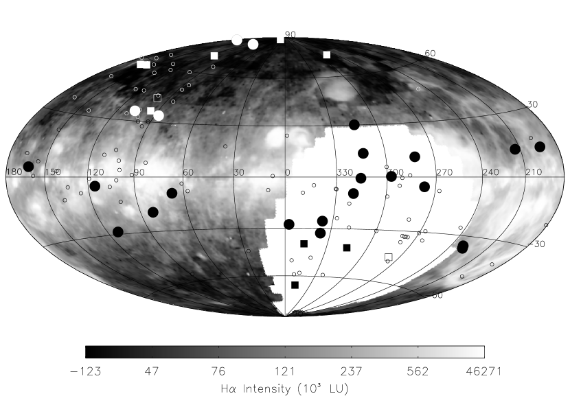
Figure 6: FUSE O VI emission survey sight lines overlaid on a WHAM map. Symbols and projection are the same as in Figure 1.

Figure 6 shows a map of H$\alpha$ emission produced from the Wisconsin H-Alpha Mapper (WHAM) survey (Haffner et al., 2003) overlaid with the positions of our survey sight lines and previously published sight lines. We used the Southern H-Alpha Sky Survey Atlas (SHASSA; Gaustad et al., 2001) to look for H$\alpha$ features in the area not covered by the WHAM survey. SHASSA has a higher resolution than the WHAM survey, but less sensitivity, so faint structures in the ionized gas cannot be indentified with SHASSA. According to the WHAM and SHASSA maps, O VI emission is detected in all environments, i.e., toward H II regions, filaments, and bubbles as well as faint, featureless ionized gas. Tables 2–The Far Ultraviolet Spectroscopic Explorer Survey of O VI Emission in the Milky Way include the H$\alpha$ intensities integrated over the velocity range of $-80$ km s${}^{-1}<v<+80$ km s^-1 measured by WHAM.

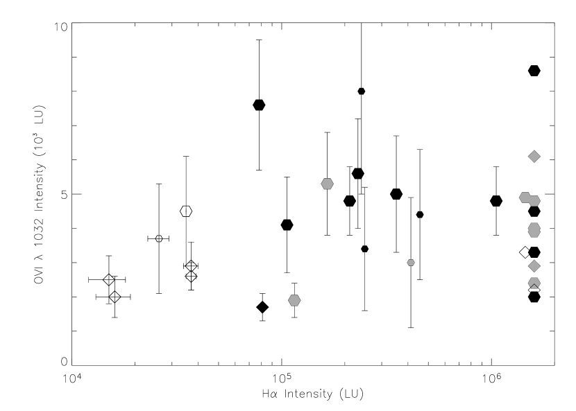
Figure 7: Comparison between O VI and H$\alpha$ intensities. Only detection sight lines are plotted. Hexagons mark the survey sight lines, diamonds represent published sight lines from the literature. Black symbols show detections toward structures in H$\alpha$ emission (e.g., filaments, H II regions) in the disk, gray and open symbols represent sight lines probing diffuse gas in the disk and halo, respectively. The smaller symbols mark sight lines with $I/\sigma_{\rm I}<2.7$. Sight lines not included in the WHAM survey are plotted at the right side of the graph without error bars for completeness. The O VI intensities for these sight lines are the measured values, but their H$\alpha$ intensity has no meaning.

Savage et al. (2003) found that O VI absorption and H$\alpha$ emission are poorly correlated. In Fig. 7, we compare the measured O VI $\lambda 1032$ intensities with the H$\alpha$ intensities for all sight lines observable by WHAM. The two instruments used different size apertures (a square of 900 arcsec²=0.25 arcmin² for FUSE, a one-degree diameter or 2827 arcmin² beam for WHAM); however, on a global (Galactic) scale, a comparison between these two data sets is still useful. We divided the sight lines into three groups represented by the differently shaded symbols in Fig. 7: black symbols indicate sight lines that probe H$\alpha$ structures like filaments or bubbles in the Galactic disk (i.e., $|b|<45\arcdeg$), gray and open symbols represent sight lines through diffuse gas in the disk and halo, respectively. Our survey does not include sight lines toward H$\alpha$ structures in the halo (i.e., at $|b|>45\arcdeg$). (The H$\alpha$ morphology along our 23 detection sight lines is described in Table 5.)

Lower latitude sight lines most likely probe gas in the disk, since absorption at low $b$ should prevent longer path lengths and thus the probing of halo gas. In addition, H$\alpha$ features like filaments or bubbles can be clues that different processes are at work in those regions than in diffuse, featureless gas. We therefore calculated the average O VI and H$\alpha$ intensities for the three groups of sight lines defined above. Combining the measurements from Tables 2 and The Far Ultraviolet Spectroscopic Explorer Survey of O VI Emission in the Milky Way (that are covered by the WHAM survey) yields an average O VI intensity of gas with H$\alpha$ structures in the disk of $\bar{I}=4800\pm 300$ LU (with a SD of 1800 LU around the mean). For diffuse gas, $\bar{I}=3600\pm 1200$ LU (SD: 2400 LU) in the disk and $2900\pm 200$ LU (SD: 1000 LU) in the halo. Again, no H$\alpha$ features are observed along halo sight lines. The average H$\alpha$ intensities for these categories are $3.0\pm 0.5\times 10^{5}$ LU (SD: $3.5\times 10^{5}$ LU), $1.4\pm 0.2\times 10^{5}$ LU (SD: $3.5\times 10^{4}$ LU), and $2.8\pm 0.2\times 10^{4}$ LU (SD: $1.1\times 10^{4}$ LU), respectively. Both average O VI and H$\alpha$ intensities are lowest for the halo sight lines and highest for the disk gas that exhibits H$\alpha$ features. The halo sight lines clearly occupy a distinct area in Fig. 7. Including the sight lines for which no WHAM data exist yields an average O VI intensity toward H$\alpha$ structures in the disk of $4700\pm 600$ LU (SD: 2100 LU) and, for diffuse gas, $\bar{I}=4000\pm 500$ LU (SD: 1400 LU) in the disk and $2900\pm 300$ LU (SD: 800 LU) in the halo.

The FUSE and WHAM instruments possess different velocity resolutions (106 km s^-1 for the FUSE LWRS aperture, 2 km s^-1 for WHAM). Most of the H$\alpha$ emission falls within one resolution element of the FUSE observation. We therefore cannot distinguish individual components in the O VI line profile; only the bulk emission can be compared in the velocity range covered by WHAM ($|v_{\rm LSR}|\approx 100$ km s^-1). Of the 14 sight lines for which WHAM data exist, the O VI emission line fully overlaps the H$\alpha$ emission in 11 of them. Eight of these show differences between the O VI and H$\alpha$ emission line centers of less than 25 km s^-1. The remaining three sight lines exhibit differences between 35 and 60 km s^-1. Thus, the O VI and H$\alpha$ emission features appear to have similar velocities along 2/3 of the sight lines (where data are available), but FUSE lacks the velocity resolution to conclude how much of the H$\alpha$ emission originates in the same cloud as the O VI emission.

Several comparisons between model predictions and observed column densities of high-ionization species like O VI and C IV have been published (e.g., Sembach & Savage, 1992; Sembach, 1993; Spitzer, 1996; Indebetouw & Shull, 2004b). Very few models, unfortunately, make predictions about O VI emission. Under the simplifying assumption that all of the O VI and H$\alpha$ emission along each sight line originates in the same gas cloud, we compared their intensities with those predicted by models of turbulent mixing layers (TML) and cooling Galactic Fountain gas. Slavin, Shull, & Begelman (1993) give O VI and H$\alpha$ intensities for TML models of different abundances, temperatures, and velocities. The predicted H$\alpha$ intensities vary between 35 and 800 LU, the O VI intensities go up to about 12 LU. This means that the predicted TML intensities are several orders of magnitude smaller than the observed ones. Benjamin & Shapiro (1996, private communication) predict H$\alpha$ intensities for clouds of various sizes of cooling Galactic Fountain gas between 2 and $2.5\times 10^{4}$ LU, which is the intensity range covered by our halo sight lines. The corresponding O VI intensities, however, are between 2 and $3\times 10^{4}$ LU, i.e. about ten times higher than the observed intensities of the halo sight lines. Correcting the observations for the low attenuation toward the halo cannot explain this discrepancy. A single model therefore cannot explain the observed O VI intensities. Absorption line studies (e.g., Spitzer, 1996; Indebetouw & Shull, 2004b) also concluded that mixed models are necessary to explain the observed O VI column densities.

5.3 Comparison between O VI and Soft X-Ray Emission

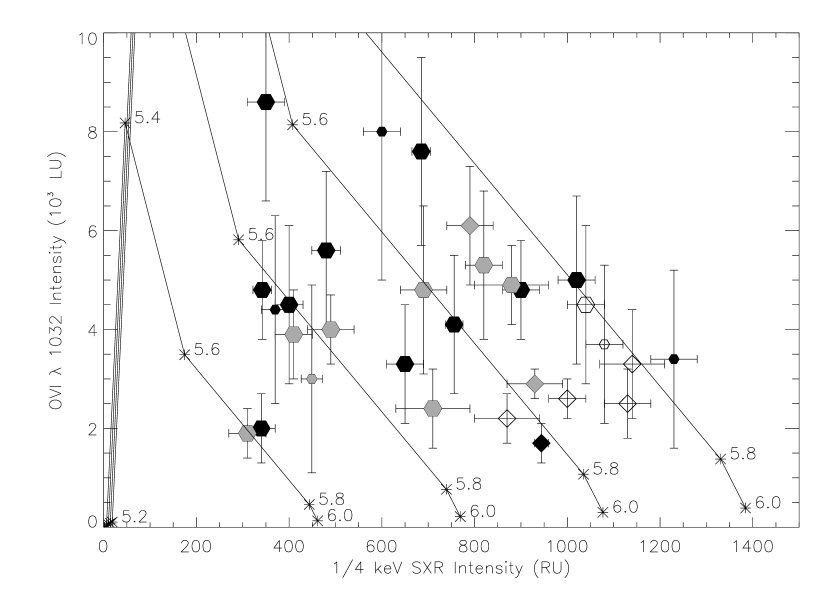
Figure 8: Comparison between O VI and SXR emission. Symbols are the same as in Figure 7. Only detection sight lines are shown. Sight lines SL1 and SL2 (Table The Far Ultraviolet Spectroscopic Explorer Survey of O VI Emission in the Milky Way) are not included (see text). The lines combine intensities (asterisks) derived from the computed thermal spectra of Landini & Monsignori Fossi (1990) for emission measures 0.015, 0.025, 0.035, and 0.045 cm^-6 pc (increasing toward the upper right). The model intensities are labelled with their corrsponding temperatures $\log(T)$.

One possible origin of the O VI emission is gas cooling from temperatures of $10^{6}$ K or more. Such hot gas is observable in the SXR regime. In Fig. 8, we compare the measured O VI $\lambda$1032 intensities with the ROSAT 1/4 keV SXR emission. Two of the O VI detections of Table The Far Ultraviolet Spectroscopic Explorer Survey of O VI Emission in the Milky Way (SL1 and SL2) are not included in the plot, as their unusually strong SXR emission probably includes emission from the galaxy clusters located in these directions.

If we divide the SXR data from Tables 2 and The Far Ultraviolet Spectroscopic Explorer Survey of O VI Emission in the Milky Way (excluding SL1 and SL2) into three bins with an equal number of sight lines, the resulting bins cover the SXR intensity ranges $<599$, 600–899, and $>900$ RU (ROSAT unit; 1 RU = $10^{-6}$ counts s^-1 arcmin^-2). The mean O VI intensities for each bin are $4400\pm 800$ LU (SD: 2100 LU), $4500\pm 600$ LU (SD: 1700 LU), and $3400\pm 400$ LU (SD: 1200 LU). Although the scatter in the data is large, there appears to be a decrease in O VI intensity in the regions of strongest SXR emission. If we divide the sight lines again into the three categories mentioned in § 5.2 (disk gas with and without H$\alpha$ features, diffuse halo gas) and exclude SL1 and SL2, the SXR intensities are $620\pm 80,670\pm 70$, and $1040\pm 50$ RU with SDs of 260, 220, and 110 RU, respectively. The average O VI intensity of this sample of halo sight lines is $3000\pm 400$ LU with a SD of 900 LU, i.e., only slightly different from the value mentioned in § 5.2. Again, the areas of strongest SXR emission exhibit the lowest O VI intensities.

Landini & Monsignori Fossi (1990) computed spectra emitted by hot ($10^{4}-10^{8}$ K), optically thin gas for the X-ray and ultraviolet wavelength regime assuming collisional ionization equilibrium. We derived SXR and O VI intensities from their tables for various temperatures and emission measures (using a conversion factor of $5.8\times 10^{-12}$ ergs cm^-2 count^-1 for the ROSAT SXR counts; Fleming et al., 1996). The lines in Fig. 8 show the resulting O VI and SXR intensities for emission measures of 0.015, 0.025, 0.035, and 0.045 cm^-6 pc for various temperature values $\log(T)$. Observations along the sight lines probing diffuse gas in the disk lie mostly in the central part of the parameter space in Fig. 8, while the observations toward the halo occupy the high SXR/low O VI intensity region. A comparison between the model by Landini & Monsignori Fossi (1990) and the data is problematic mainly for three reasons: 1) The model assumption of collisional ionization equilibrium does not apply to cooling and possibly condensing Galactic Fountain gas. 2) The observed data in the disk are affected by attenuation, a correction of which may change the distribution of the data points in Fig. 8. While attenuation certainly has an effect on the lower latitude sight lines (see § 5.6 below), it cannot explain the drop in O VI emission for the halo sight lines. 3) The SXR intensities contain a contribution from the Local Bubble, whereas the amount of O VI emission from the Local Bubble is still being debated. Despite these drawbacks in our comparison, however, it is comforting to see that the predicted and observed intensities are of the same order of magnitude – unlike the models in the O VI–H$\alpha$ comparison in § 5.2 above.

5.4 Galactic Rotation

Table 2 includes the local-standard-of-rest velocities $v_{\rm LSR}$ for all O VI $\lambda$1032 detections. To compare these velocities with Galactic rotation, we adopted a simple rotation model, a differentially corotating halo with a constant velocity of $v=220$ km s^-1. We derived the distance $D$ along the line of sight to the O VI emitting gas and its height $z$ above the Galactic plane from the match between the model and the measured velocity. The values for $z$ and $D$ derived from our model are listed in Table 5. The quoted uncertainties in $z$ and $D$ are based on the overlap between the 1$\sigma$ uncertainties of the measured velocities and the velocities allowed by the corotation model. If a match between the measured velocity and the model exists only within the uncertainty of the velocity, the values for $z$ and $D$ are quoted as ranges. For sight lines with $0\arcdeg<l<90\arcdeg$ or $270\arcdeg<l<360\arcdeg$, two solutions might exist for a part of or the full 1$\sigma$ range, as the velocity contours of the corotation model loop around inside the solar orbit around the Galactic center. There are a handful of sight lines for which no solution exists within the observed 1$\sigma$ range. Two sight lines yield solutions up to the end of the Galactic disk/halo (represented by question marks in Table 5, since the “exact” end of the disk/halo is not known). Figure 9 shows the model velocity profiles, the measured velocities, and their uncertainty ranges for three survey detection sight lines as an example. The model velocities were always calculated for $D=0-20$ kpc without consideration of the direction of the sight line.

The measured velocities of seven of the 23 sight lines are inconsistent with the corotating halo model (e.g., measured $v_{\rm LSR}>0$ in $v_{\rm halo}<0$ region or vice versa). The other sight lines (about 2/3 of the detection sight lines) yield solutions of various likelihoods. These depend on the probability of the observed velocity and the derived values for $|z|$ and $D$ with regard to the expected extinction along and the direction of the sight line. For sight lines with two solutions, for example, the first listed solution is usually more likely due to the higher extinction along the longer path length and the larger (and sometimes unreasonable) values for $|z|$ or $D$ of the second solution. The comment in Table 5 takes these probabilities into account and describes what we believe is the likely range of the corotating, emitting gas. We define “local” as $D\leq 500$ pc, “near” as $D\leq 5$ kpc, and (thick) disk gas as $|z|\leq 2.3$ kpc. All sight lines yielding solutions for the corotation model place the emitting gas in the near disk, in a few cases even in the local environment. None of the sight lines yields only a halo solution (with halo now defined as $|z|>2.3$ kpc) without a near disk solution.

The measured velocities vary particularly strongly toward the northern Galactic pole ($b>60\arcdeg$). Combining the detections of Tables 2 and The Far Ultraviolet Spectroscopic Explorer Survey of O VI Emission in the Milky Way, we find five sight lines that fall into that region: S40581 ($l=110\fdg 3$, $I/\sigma_{\rm I}=2.3$), S40508 ($l=175\fdg 0$), SL1, SL2, and SL4. Positive as well as negative O VI $\lambda$1032 velocities are measured in this direction, suggesting that turbulence, outflow, and infall play an important role in the distribution of the O VI-emitting gas. One caveat, however, is the low spectral resolution of our 106 km s^-1 wide aperture, which would be unable to resolve the emission from multiple clouds along the line of sight (due to the strong binning of the data). If multiple clouds were present, the derived values for $v_{\rm LSR}$ would represent an average for each sight line.

5.5 High-Velocity Clouds

A large number of high-velocity ($|v|>100$ km s^-1) components was detected in the O VI absorption survey of Sembach et al. (2003). The majority of these components was observed toward high-velocity H I 21 cm emission. Using the maps of high-velocity H I gas in Wakker et al. (2003, their Fig. 16) and Sembach et al. (2003, their Fig. 11), we identified the sight lines in our O VI emission survey that intersect H I HVCs. Almost half of the sight lines in our survey (52 out of 112) pass regions of high-velocity H I gas, yet of the 23 sight lines showing O VI emission, only five intersect H I HVCs (all with $I/\sigma_{\rm I}\geq 2.7$). In none of these cases do the measured O VI and H I velocities agree ($|v_{\rm OVI}-v_{\rm HI}|>50$ km s^-1); however, we have found one region of the sky that exhibits O VI emission and absorption at similar velocities. Sight line S40521 ($l=81\fdg 9$, $I/\sigma_{\rm I}=2.3$) shows a weak emission line at $v_{\rm LSR}=-320\pm 30$ km s^-1. Three nearby absorption sight lines, Mrk1513, Mrk304, and UGC12163, exhibit high-velocity O VI components at $v_{\rm LSR}=-293,-304,$ and $-274$ km s^-1, respectively. Sembach et al. (2003) identify this region as an extension of the Magellanic Stream. Except for this region of the Magellanic Stream, our survey does not contain any sight lines near HVCs originally detected in high-ionization species such as C IV or O VI and studied by Sembach et al. (1995, 2003) and Collins, Shull, & Giroux (2005). Detecting O VI emission from HVCs appears more difficult than detecting diffuse O VI emission – given the fact that none of the 52 sight lines that pass regions of H I HVCs exhibits O VI emission from the HVC. In their extended survey, Dixon et al. (2006) found two (of a total of 183) sight lines with high-velocity O VI emission matching the high-velocity H I emission.

5.6 Variation in Extinction and O VI Intensity with Galactic Latitude

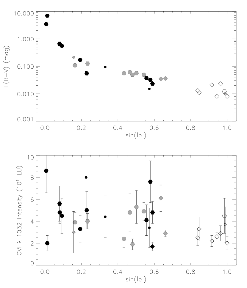
Figure 10: Upper panel: Variation of $E(\bv)$ with Galactic latitude. Lower panel: Variation of O VI intensity with Galactic latitude. Symbols are the same as in Figure 7. Only detection sight lines are shown.

When analyzing emission measurements in the ultraviolet, it is important to consider the effects of interstellar extinction. A plot of the color excess $E(B-V)$ versus $\sin(|b|)$ (where $b$ is the Galactic latitude) for sight lines showing O VI emission is presented in the upper panel of Fig. 10. The sharp decrease in dust extinction with Galactic latitude is obvious. The high color excess at low latitudes suggests strongly that the O VI emission is local (that is, closer than the obscuring dust).

The observed O VI $\lambda$1032 intensities are plotted against $\sin|b|$ in the lower panel of Fig. 10. For the nine high signal-to-noise sight lines with $\sin|b|<0.4$, the average intensity is $4600\pm 600$ LU (SD: 1800 LU). For the 11 sight lines with $0.4<\sin|b|<0.7$, the average intensity is $4200\pm 600$ LU (SD: 1800 LU). For the seven remaining sight lines, with $\sin|b|>0.7$, the average intensity is $2900\pm 300$ LU (SD: 800 LU). We see that, at high latitudes, the intensities are lower and the dispersion decreases. Based on these plots, we divide our sample into low-latitude, mid-latitude, and high-latitude sight lines. While both extinction and observed O VI intensity fall with increasing Galactic latitude for our complete sample, within each group we see no correlation of the observed O VI intensity with reddening.

The relatively low dispersion in the intensities of our high-latitude sight lines suggests that they sample gas with a uniform set of properties. The O VI emission observed at these latitudes is thus likely to be from hot gas in the thick disk/halo. The low-latitude sight lines are significantly brighter than at higher latitudes, even though their extinction is higher; hence, the low-latitude emission must come from nearby regions, probably interfaces in the thin disk, as suggested by the absorption data. The average intensity for the mid-latitude sight lines lies between the averages for the high and low-latitude sight lines. This is simply explained if at these latitudes the sight lines pass through both nearby emission interfaces and more distant O VI in the thick disk. The dispersion then reflects the clumpiness of the hot gas in the Galaxy.

6 CONCLUSIONS

We have examined 112 sight lines from the FUSE archive that probe diffuse, hot gas in the Milky Way and found 23 that exhibit O VI $\lambda$1032 emission. Sight lines crossing morphological features like H$\alpha$ filaments or bubbles in the disk exhibit the strongest O VI emission. Halo sight lines show the lowest O VI and H$\alpha$ intensities, the strongest SXR emission, and little or no H$\alpha$ structure. This suggests that different mechanisms are at work in areas that show morphological features as opposed to purely diffuse gas. Higher O VI intensities toward H$\alpha$ filaments and bubbles indicate that the O VI emission originates in interfaces or turbulent mixing layers. Neither TML nor Galactic Fountain models can reproduce the observed intensities. Data derived from computed thermal X-ray/UV spectra, however, are consistent with our observations for a range of emission measures and temperatures. About 2/3 of our detection sight lines probe clouds whose velocities are consistent with a corotating halo, placing the emitting gas most likely within a few kpc in the thick disk, if not locally within only a few 100 pc from the sun. Sight lines toward the northern Galactic pole ($b>60\arcdeg$) show velocities that differ from the corotation model and indicate turbulences, outflows, or infall of gas. None of our sight lines shows O VI emission originating in H I HVCs. Only one sight line possesses O VI emission coinciding with the detection of high-velocity O VI absorption toward the extension of the Magellanic Stream. Combined with values from the literature, the O VI intensities from our survey exhibit a variation with latitude that is consistent with the picture derived from recent O VI absorption measurements: high-latitude sight lines probe O VI-emitting gas in a clumpy, thick disk, while low-latitude sight lines sample mostly mixing layers and interfaces in the thin disk of the Galaxy. By combining O VI intensities with column densities derived from absorption-line surveys, we can constrain the local density and physical scale of the emitting gas. The challenge is finding suitable emission/absorption measurements due to the clumpy nature of the O VI-bearing gas. Theoretical models of this phase of the interstellar medium in the Galaxy must reproduce both the large-scale distribution of O VI emission and the small-scale microphysics derived from O VI emission and absorption surveys. No single model can explain the observed emission and absorption data at this point.

Table 1: OBSERVATIONS

Target ID	Observation IDs
A01002	A0100201
A03406	A0340601
A03407	A0340701
A04604	A0460404
A04802	A0480202
A04905	A0490501, A0490502
A05101	A0510102
A10001	A1000101
A11101	A1110101
A11102	A1110201
B01805	B0180501
B04604	B0460401, B0460501
B06801	B0680101
B09401	B0940101
C02201	C0220101, C0220102
C02301	C0230101
C03701	C0370101
C03702	C0370201, C0370202, C0370203, C0370204, C0370205
C05501	C0550101
C07602	C0760201, C0760301
C07604	C0760401
M10310	M1031003, M1031004, M1031006, M1031007
M10703	M1070301, M1070302, M1070304, M1070305, M1070307, M1070308,
	M1070310, M1070311, M1070313, M1070314, M1070319
P10407	P1040701
P10409	P1040901
P10411	P1041101, P1041102, P1041103
P10413	P1041303
P10414	P1041403
P10418	P1041801
P10425	P1042501, P1042601
P12012	P1201112, P1201213
P20406	P2040601
P20410	P2041002, S4053601
P20411	P2041102, P2041103, P2041104
P20419	P2041901
P20421	P2042101
P20422	P2042201, P2042202, P2042203, S4055602, S4055603, S4055607,
	S4055608, S4055609
P20423	P2042301
P20517	P2051701, P2051702, P2051703
Q10803	Q1080303
Q11002	Q1100201
S30402	S3040203, S3040204, S3040205, S3040206, S3040207, S3040208
S40502	S4050201
S40504	S4050401
S40505	P1042101, P1042105, S4050501, S4050502, S4050503
S40506	S4050601
S40507	S4050701
S40508	S4050801
S40509	S4050903
S40510	S4051001, S4051002
S40512	S4051201
S40513	S4051301
S40514	S4051401
S40518	S4051801, S4051802, S4051803, S4051804, S4051805
S40521	S4052101
S40522	S4052201
S40523	S4052301, S4052302
S40524	S4052402, S4052403, S4052404, S4052405, S4052406
S40525	S4052501
S40526	S4052601
S40529	S4052901, S4052902
S40531	S4053101
S40532	S4053201, S4053202
S40533	S4053301
S40535	S4053501
S40537	S4053701, S4053702
S40540	S4054001, S4054002, S4054003, S4054004, S4054005
S40541	S4054101
S40543	S4054301
S40553	S4055301
S40555	S4055501, S4055502
S40557	S4055701, S4055702, S4055703, S4055704, S4055705
S40558	S4055801
S40560	S4056001, S4056002
S40562	S4056201
S40563	S1010206, S4056301, S4056302, S4056303, S4056304
S40564	S4056401
S40566	S4056601, S4056602, S4056603
S40568	S4056801, S4056802
S40569	S4056901
S40570	S4057001
S40572	S4057201
S40573	S4057301, S4057302
S40574	S4057401
S40576	S4057601, S4057602, S4057603, S4057604
S40579	P1042901, P1042902, S4057901, S4057902, S4057903, S4057904
S40580	S4055001, S4058001
S40581	S4058101, S4058102
S40582	S4058201, S4058202
S40587	S4058701
S40588	S4058801
S40589	S4058901
S40590	S4059001
S40591	S4059101
S40593	S4059301
S51303	S5130301
S51401	S5140102, S5140103
Z90702	Z9070201
Z90703	Z9070301
Z90708	Z9070801
Z90709	Z9070901
Z90711	Z9071101
Z90712	Z9071201
Z90714	Z9071401
Z90715	Z9071501
Z90719	Z9071901
Z90726	Z9072601, Z9072602
Z90727	Z9072701
Z90732	Z9073202
Z90735	Z9073501
Z90736	Z9073601
Z90737	Z9073701, Z9073702

Table 2: O VI $\lambda$1032 MEASUREMENTS

Target	$l$	$b$	$t$	$I_{1032}$	$\lambda_{\rm c}$	FWHM		$1-P_{\rm F}$	$v_{\rm LSR}$		SXR	$I_{{\rm H}\alpha}$
ID	(deg.)	(deg.)	(sec)	(103 LU)	(Å)	(km s-1)	$\chi^{2}/\nu$	(%)	(km s-1)	$E(B-V)$	(RU)	(103 LU)	HVC
S40523	67.219	$-9.024$	9820	$3.0\pm 1.9$	$1031.98\pm 0.13$	$120\pm 150$	0.94	56	$30\pm 40$	0.213	$449\pm 23$	$413\pm 4$	—
S40521	81.875	$-19.293$	13539	$4.4\pm 1.9$	$1030.78\pm 0.10$	$140\pm 90$	1.08	66	$-320\pm 30$	0.094	$370\pm 30$	$456\pm 0$	—
S40560	87.172	$+33.829$	19249	$4.1\pm 1.4$	$1031.86\pm 0.07$	$110\pm 80$	1.38	73	$-3\pm 19$	0.037	$756\pm 19$	$106\pm 4$	C
Z90715	106.808	$+35.314$	14576	$7.6\pm 1.9$	$1031.85\pm 0.10$	$200\pm 30$	1.61	76	$-10\pm 30$	0.032	$685\pm 20$	$78\pm 3$	C
S40581	110.308	$+81.653$	14330	$3.7\pm 1.6$	$1031.70\pm 0.18$	$180\pm 120$	0.95	66	$-60\pm 50$	0.010	$1080\pm 40$	$26\pm 3$	—
P20411	112.482	$-28.688$	48281	$1.9\pm 0.5$	$1031.82\pm 0.04$	$4\pm 80$	0.89	75	$-25\pm 12$	0.049	$310\pm 40$	$115\pm 3$	—
S30402	115.438	$-4.644$	30491	$4.8\pm 1.0$	$1032.62\pm 0.09$	$201\pm 19$	0.82	84	$210\pm 25$	0.627	$342\pm 20$	$1054\pm 0$	H/G
P10413	162.590	$+4.566$	14644	$5.6\pm 1.6$	$1031.84\pm 0.10$	$180\pm 60$	1.00	77	$-30\pm 30$	0.667	$480\pm 31$	$231\pm 0$	—
S40508	175.036	$+80.024$	8290	$4.5\pm 1.6$	$1032.08\pm 0.09$	$110\pm 100$	0.66	79	$50\pm 30$	0.012	$1040\pm 40$	$35\pm 0$	—
P12012	194.301	$+13.230$	9680	$5.0\pm 1.7$	$1031.89\pm 0.11$	$200\pm 50$	0.94	64	$-20\pm 30$	0.055	$1020\pm 40$	$352\pm 3$	—
P10418	213.704	$+13.019$	3350	$8\pm 3$	$1031.75\pm 0.08$	$80\pm 150$	0.97	69	$-67\pm 24$	0.062	$600\pm 40$	$240\pm 0$	—
P10411	229.296	$-36.167$	46120	$4.8\pm 1.0$	$1031.96\pm 0.04$	$100\pm 50$	0.97	98	$-10\pm 12$	0.023	$900\pm 40$	$211\pm 3$	—
S40537	230.674	$-34.936$	21020	$3.4\pm 1.8$	$1031.90\pm 0.07$	$90\pm 170$	1.09	73	$-26\pm 19$	0.015	$1230\pm 50$	$249\pm 4$	—
P20517	277.041	$-5.306$	35923	$4.5\pm 1.6$	$1031.80\pm 0.11$	$190\pm 120$	1.33	73	$-50\pm 30$	0.556	$400\pm 30$	$\cdots$	—
S40506	282.142	$+11.097$	12990	$3.3\pm 1.2$	$1031.85\pm 0.09$	$80\pm 50$	1.20	62	$-30\pm 30$	0.171	$650\pm 40$	$\cdots$	WD?
S40591	297.557	$+0.337$	7131	$8.6\pm 2.0$	$1031.97\pm 0.06$	$80\pm 60$	1.21	69	$4\pm 18$	3.417	$350\pm 40$	$\cdots$	—
S40557	313.373	$+13.487$	48836	$4.0\pm 0.7$	$1031.74\pm 0.03$	$77\pm 23$	0.96	98	$-57\pm 10$	0.126	$490\pm 50$	$\cdots$	—
A04604	314.861	$+30.105$	18147	$5.3\pm 1.5$	$1031.91\pm 0.07$	$160\pm 60$	1.09	79	$-4\pm 21$	0.056	$820\pm 40$	$165\pm 3$	—
P10425	315.732	$-0.679$	26568	$2.0\pm 0.7$	$1031.92\pm 0.06$	$10\pm 180$	1.04	67	$-4\pm 16$	6.950	$340\pm 30$	$\cdots$	WE?
S40590	319.714	$-9.448$	10914	$3.9\pm 0.9$	$1031.81\pm 0.04$	$10\pm 40$	0.88	78	$-37\pm 12$	0.108	$410\pm 40$	$\cdots$	—
C07602	336.501	$-25.677$	33042	$2.4\pm 0.8$	$1031.89\pm 0.06$	$50\pm 50$	1.44	69	$-10\pm 18$	0.056	$710\pm 80$	$\cdots$	—
P20422	336.583	$-32.859$	76990	$4.9\pm 0.8$	$1031.87\pm 0.04$	$140\pm 30$	1.13	99	$-17\pm 11$	0.049	$880\pm 80$	$\cdots$	—
S40568	357.478	$-27.762$	11912	$4.8\pm 1.7$	$1031.94\pm 0.11$	$180\pm 80$	1.16	64	$9\pm 30$	0.061	$690\pm 50$	$\cdots$	—

Table 3: O VI $\lambda$1032 3$\sigma$ UPPER LIMITS

Target	$l$	$b$	$t$	$I_{1032}$		SXR	$I_{{\rm H}\alpha}$
ID	(deg.)	(deg.)	(sec)	(103 LU)	$E(B-V)$	(RU)	(103 LU)	HVC
S40512	7.153	$+0.616$	4280	$4$	7.919	$310\pm 40$	$2583\pm 5$	—
Q10803	9.876	$-7.555$	3977	$3$	0.331	$270\pm 30$	$748\pm 4$	—
P20406	27.361	$-43.759$	18938	$1.9$	0.047	$720\pm 40$	$75\pm 0$	—
S40525	36.064	$+17.621$	2840	$4$	0.193	$440\pm 30$	$225\pm 3$	C/D
S40533	57.538	$-7.929$	5361	$3$	0.301	$540\pm 30$	$424\pm 4$	—
M10703	60.838	$-3.696$	59975	$2.4$	1.415	$560\pm 30$	$622\pm 0$	—
S40566	83.328	$+7.756$	20569	$2.0$	0.459	$488\pm 18$	$1794\pm 5$	—
C03701	84.517	$+42.189$	29877	$1.2$	0.006	$1410\pm 40$	$38\pm 0$	C
S40555	85.357	$+52.349$	13661	$1.8$	0.016	$1230\pm 30$	$35\pm 0$	C
Z90735	86.917	$+49.393$	18113	$2.3$	0.015	$1180\pm 30$	$42\pm 0$	C
Q11002	86.983	$+64.666$	8380	$2.5$	0.010	$1270\pm 30$	$33\pm 0$	—
C03702	88.217	$-55.564$	71065	$0.9$	0.052	$420\pm 30$	$47\pm 0$	MS
S40518	91.373	$+1.134$	30450	$1.4$	2.787	$434\pm 22$	$1552\pm 4$	—
Z90736	91.820	$+30.217$	27775	$1.6$	0.041	$725\pm 10$	$61\pm 3$	C
M10310	94.027	$+27.428$	12798	$2.3$	0.043	$712\pm 9$	$147\pm 3$	—
P20410	98.733	$+29.775$	19748	$1.6$	0.054	$619\pm 8$	$115\pm 3$	C
B04604	99.293	$+3.738$	10076	$2.6$	0.963	$283\pm 16$	$14237\pm 0$	—
S40524	100.514	$+8.623$	42076	$1.0$	1.009	$314\pm 16$	$2574\pm 6$	—
S40564	100.608	$-13.070$	5080	$2.3$	0.264	$240\pm 18$	$320\pm 0$	G
S40543	100.787	$+44.753$	10636	$2.2$	0.032	$970\pm 30$	$31\pm 0$	C
S40532	101.243	$-1.686$	18310	$1.7$	0.537	$252\pm 17$	$1518\pm 5$	G
Z90711	101.294	$+32.279$	21733	$1.8$	0.034	$688\pm 13$	$83\pm 3$	C
B01805	101.785	$+59.630$	4164	$4$	0.010	$1330\pm 40$	$35\pm 3$	C
Z90714	103.875	$+36.157$	11051	$3$	0.043	$554\pm 14$	$88\pm 3$	C
A05101	104.063	$+14.193$	14883	$1.7$	11.928	$357\pm 20$	$361\pm 4$	—
S40522	105.720	$-5.122$	3969	$4$	0.399	$260\pm 30$	$897\pm 4$	G
A03406	110.865	$+11.487$	1600	$5$	0.702	$460\pm 30$	$699\pm 4$	—
S40579	111.297	$+33.579$	67002	$1.1$	0.041	$583\pm 22$	$56\pm 3$	—
S40510	117.187	$+46.348$	28645	$1.3$	0.012	$1090\pm 30$	$9\pm 4$	C
S40535	119.019	$-0.893$	3680	$4$	1.696	$410\pm 40$	$2331\pm 0$	H
Z90709	123.725	$+58.782$	8067	$4$	0.011	$1170\pm 40$	$14\pm 2$	C
Z90712	125.299	$+46.300$	5474	$4$	0.018	$1000\pm 30$	$60\pm 3$	C
C02201	125.618	$-8.037$	17556	$2.4$	0.416	$440\pm 50$	$602\pm 4$	H
S40505	133.117	$+55.658$	37331	$1.4$	0.015	$900\pm 50$	$19\pm 2$	C
S40529	133.963	$-4.989$	11836	$2.3$	0.413	$378\pm 22$	$443\pm 3$	H
S40562	134.391	$+61.764$	14440	$1.6$	0.015	$850\pm 40$	$38\pm 2$	C?
S40570	138.060	$-11.120$	13778	$2.0$	0.162	$530\pm 30$	$410\pm 3$	H
S40580	141.384	$+32.628$	15066	$1.8$	0.028	$610\pm 30$	$73\pm 3$	A
S40572	141.499	$+2.878$	13700	$2.1$	1.318	$287\pm 21$	$1285\pm 0$	H
S40588	150.639	$+58.933$	12401	$2.1$	0.017	$1100\pm 50$	$16\pm 3$	C?
Z90727	151.433	$+22.123$	2960	$4$	0.092	$440\pm 30$	$114\pm 3$	—
S40576	155.955	$+7.099$	29845	$1.4$	0.593	$320\pm 30$	$213\pm 3$	—
S40502	158.488	$+0.472$	5672	$3$	1.174	$330\pm 30$	$1359\pm 4$	—
S40574	159.921	$+58.496$	7510	$2.4$	0.020	$910\pm 30$	$40\pm 3$	C
S40587	161.916	$+64.733$	8390	$2.3$	0.014	$1210\pm 40$	$27\pm 3$	M
S40540	164.067	$+49.004$	14779	$1.9$	0.010	$1000\pm 40$	$66\pm 4$	A
S40541	164.817	$+36.961$	2290	$4$	0.038	$610\pm 50$	$54\pm 0$	A
Z90732	165.287	$+61.408$	10347	$4$	0.012	$1420\pm 40$	$36\pm 3$	—
P10414	166.158	$+10.475$	7960	$3$	0.234	$330\pm 30$	$365\pm 3$	—
S40513	178.879	$+59.009$	12260	$2.4$	0.014	$1500\pm 50$	$31\pm 3$	M
P10409	180.973	$-20.249$	11883	$2.3$	0.587	$450\pm 30$	$813\pm 0$	AnCen
S40531	188.956	$-40.098$	5910	$3$	0.188	$710\pm 30$	$1402\pm 4$	—
P10407	195.846	$-48.051$	27675	$1.3$	0.039	$1490\pm 60$	$476\pm 0$	—
S40504	197.880	$+17.400$	1635	$5$	0.051	$1680\pm 50$	$397\pm 3$	—
A03407	243.721	$-26.124$	8150	$3$	0.036	$770\pm 30$	$\cdots$	—
S40509	247.554	$+47.752$	5721	$3$	0.076	$550\pm 30$	$228\pm 4$	WA?
S40573	264.191	$-34.510$	21100	$1.8$	0.040	$620\pm 40$	$\cdots$	W?
Z90726	266.478	$-29.397$	21110	$1.7$	0.046	$504\pm 16$	$\cdots$	—
A04802	267.366	$-7.476$	6300	$4$	0.965	$555\pm 22$	$\cdots$	—
S40582	270.079	$-30.615$	21403	$1.8$	0.052	$451\pm 15$	$\cdots$	—
C05501	276.101	$-33.239$	9470	$3$	0.075	$573\pm 14$	$\cdots$	MS
Z90719	276.177	$-47.638$	10390	$3$	0.074	$780\pm 40$	$\cdots$	MS
A11102	277.764	$-33.014$	4240	$6$	0.075	$599\pm 12$	$\cdots$	MS
A11101	277.767	$-33.023$	4230	$6$	0.075	$599\pm 12$	$\cdots$	MS
A04905	278.649	$-33.170$	2738	$5$	0.075	$537\pm 11$	$\cdots$	MS
S40593	278.892	$-36.323$	5561	$4$	0.075	$522\pm 16$	$\cdots$	MS
B09401	280.309	$-32.795$	4200	$5$	0.075	$701\pm 20$	$\cdots$	MS
P20421	281.621	$-23.493$	4582	$4$	0.224	$660\pm 30$	$\cdots$	MS
S51303	286.148	$+0.957$	3444	$5$	1.088	$360\pm 40$	$\cdots$	—
S40553	290.948	$-0.488$	11878	$2.5$	1.412	$300\pm 30$	$\cdots$	—
S40507	292.316	$-4.829$	14362	$3$	0.800	$290\pm 23$	$\cdots$	—
S40558	295.613	$-0.240$	7390	$3$	3.527	$430\pm 30$	$\cdots$	WD?
S51401	299.156	$-10.943$	11553	$3$	0.238	$190\pm 30$	$\cdots$	WE?
A01002	299.854	$-30.679$	2030	$4$	0.080	$650\pm 30$	$\cdots$	—
B06801	300.171	$+5.650$	12110	$3$	0.835	$360\pm 40$	$\cdots$	WD?
S40589	318.630	$-29.168$	9854	$2.1$	0.115	$470\pm 60$	$\cdots$	—
A10001	321.537	$-15.259$	9412	$2.3$	0.102	$480\pm 60$	$\cdots$	WE
Z90708	322.827	$-58.853$	12420	$4$	0.011	$1250\pm 60$	$\cdots$	MS
Z90737	327.712	$-23.823$	29401	$1.5$	0.084	$430\pm 70$	$\cdots$	—
S40563	329.883	$-7.017$	38174	$1.5$	0.355	$460\pm 40$	$\cdots$	—
S40569	330.353	$-6.828$	10580	$1.7$	0.287	$480\pm 40$	$\cdots$	—
C07604	336.624	$-25.642$	14454	$2.3$	0.059	$680\pm 80$	$\cdots$	—
P20423	339.728	$-48.055$	4405	$4$	0.025	$2030\pm 60$	$\cdots$	—
S40526	343.165	$-4.762$	7058	$2.1$	0.554	$330\pm 30$	$\cdots$	—
C02301	346.268	$-57.954$	5700	$3$	0.009	$1190\pm 50$	$\cdots$	—
S40514	349.573	$-9.088$	11022	$3$	0.181	$280\pm 70$	$\cdots$	—
Z90703	351.251	$-58.997$	10750	$4$	0.011	$970\pm 50$	$\cdots$	—
Z90702	354.668	$-49.893$	15290	$1.8$	0.017	$960\pm 50$	$\cdots$	—
P20419	358.794	$+24.180$	14122	$2.3$	0.311	$690\pm 100$	$812\pm 4$	—

Table 4: PUBLISHED O VI $\lambda$1032 MEASUREMENTS AND 2$\sigma$ UPPER LIMITS

Target	$l$	$b$	$I_{1032}$	FWHM	$v_{\rm LSR}$		SXR	$I_{{\rm H}\alpha}$
ID	(deg.)	(deg.)	(103 LU)	(km s-1)	(km s-1)	$E(B-V)$	(RU)	(103 LU)	HVC	Ref.
SL1	57.6	$+88.0$	$2.0\pm 0.6$	$23\pm 55$	$-17\pm 9$	0.008	$4430\pm 100$	$16\pm 3$	—	1
SL2	284.2	$+74.5$	$2.9\pm 0.7$	$80$	$84\pm 15$	0.023	$5530\pm 120$	$37\pm 3$	—	1
SL3	315.0	$-41.3$	$2.9\pm 0.3$	$160$	$64$	0.036	$930\pm 60$	$\cdots$	—	2
SL4	113.0	$+70.7$	$2.6\pm 0.4$	$75$	$10$	0.008	$1000\pm 40$	$37\pm 2$	—	3
SL5	162.7	$+57.0$	$2.5\pm 0.7$	$150$	$-16\pm 22$	0.013	$1130\pm 50$	$15\pm 3$	C	4
SL6	156.3	$+57.8$	$3.3\pm 1.1$	$210$	$-50\pm 30$	0.011	$1140\pm 70$	$\cdots$	C	4
SL7	95.4	$+36.1$	$1.7\pm 0.4$	$75\pm 3$	$-50\pm 30$	0.024	$944\pm 15$	$81\pm 0$	C	5
SL8	99.3	$+43.3$	$<1.7$	$\cdots$	$\cdots$	0.034	$1160\pm 30$	$37\pm 3$	C	5
SL9	278.6	$-45.3$	$<0.5$	$\cdots$	$\cdots$	0.153	$600\pm 40$	$\cdots$	(MS)	6
SL10	348.1	$-66.3$	$2.2\pm 0.5$	$60\pm 40$	$-5\pm 9$	0.021	$870\pm 70$	$\cdots$	—	7
SL11	346.6	$-39.5$	$6.1\pm 1.2$	$140\pm 40$	$-28\pm 15$	0.035	$790\pm 50$	$\cdots$	—	7

References. — (1) Dixon et al. 2001; (2) Shelton et al. 2001; (3) Shelton 2002; (4) Welsh et al. 2002; (5) Otte et al. 2003a; (6) Shelton 2003; (7) Otte et al. 2003b

Table 5: DETECTIONS: H$\alpha$ MORPHOLOGY AND LOCATION OF O VI GAS

Target	H$\alpha$	$|z|$	$D$
ID	Morphology	(kpc)	(kpc)	Comment
S40523	diffuse	0–1.2	0–7.7	near disk
S40521	filament/blob	$\cdots$	$\cdots$	not corotating
S40560	filament	$1.4^{+2.0}_{-1.4}$	$2.4^{+3.7}_{-2.4}$	near disk
Z90715	filament	$1.0^{+2.6}_{-1.0}$	$1.8^{+4.4}_{-1.8}$	near disk
S40581	diffuse	$\cdots$	$\cdots$	not corotating
P20411	diffuse	$1.5^{+0.7}_{-0.7}$	$3.1^{+1.5}_{-1.4}$	near disk
S30402	H II	$\cdots$	$\cdots$	not corotating
P10413	blob	$0.6^{+?}_{-0.6}$	$7.4^{+?}_{-7.4}$	near disk
S40508	diffuse	$\cdots$	$\cdots$	not corotating
P12012	filament	0–0.5	0–2.1	if corotating, probably local
P10418	filament	$\cdots$	$\cdots$	not corotating
P10411	filament/bubble	0–0.1	0–0.2	local
S40537	filament/bubble	$\cdots$	$\cdots$	not corotating
P20517	bubble	$\cdots$	$\cdots$	not corotating
S40506	bubble	0–0.7	0–3.6	if corotating, local or near disk
S40591	filament/bubble	0–0.01	0–1.5	local
$\cdots$	$\cdots$	$0.05^{+0.01}_{-0.01}$	$8.2^{+1.6}_{-1.8}$	$\cdots$
S40557	diffuse	$1.2^{+0.2}_{-0.3}$	$5.3^{+0.7}_{-1.5}$	disk
$\cdots$	$\cdots$	$1.6^{+0.3}_{-0.2}$	$6.7^{+1.5}_{-0.7}$	$\cdots$
A04604	diffuse	$0.2^{+1.0}_{-0.2}$	$0.4^{+2.0}_{-0.4}$	local or near disk
$\cdots$	$\cdots$	$6.7^{+1.2}_{-1.0}$	$13.5^{+2.3}_{-2.1}$	$\cdots$
P10425	H II/blob	0.0	$0.3^{+1.2}_{-0.3}$	local
$\cdots$	$\cdots$	$0.1^{+0.1}_{-0}$	$11.9^{+1.2}_{-1.2}$	$\cdots$
S40590	diffuse	$0.4^{+0.2}_{-0.1}$	$2.6^{+0.9}_{-0.8}$	near disk
$\cdots$	$\cdots$	$1.7^{+0.2}_{-0.1}$	$10.5^{+0.8}_{-0.8}$	$\cdots$
C07602	diffuse	$0.5^{+0.7}_{-0.5}$	$1.2^{+1.6}_{-1.2}$	near disk
$\cdots$	$\cdots$	$7.0^{+1.0}_{-0.7}$	$16.1^{+2.3}_{-1.6}$	$\cdots$
P20422	diffuse	$1.2^{+0.5}_{-0.7}$	$2.1^{+1.1}_{-1.3}$	nead disk
$\cdots$	$\cdots$	$8.9^{+0.7}_{-0.5}$	$16.5^{+1.2}_{-1.1}$	$\cdots$
S40568	diffuse	0–3.2	0–6.8	local or near disk
$\cdots$	$\cdots$	5.8–?	12.3–?	$\cdots$

Figure 1: Distribution of the sight lines in the O VI emission survey. In the top panel, each sight line is labeled by its identifier used in Tables 2–The Far Ultraviolet Spectroscopic Explorer Survey of O VI Emission in the Milky Way. Galactic coordinates are used in Hammer-Aitoff projection. In the bottom panel, filled symbols represent O VI $\lambda$1032 detections; open symbols show non-detection sight lines. Circles mark the survey sight lines, squares represent previously published O VI emission sight lines. The circles for upper limit survey sight lines were reduced in size to avoid overcrowding the graph.

Figure 2: Comparison between the confidence level and the signal-to-noise ratio. The confidence level $1-P_{\rm F}$ was obtained from the F test using the ratio of the variances of the continuum fit and the emission line fit for each detection. The signal-to-noise ratio $I/\sigma_{\rm I}$ was derived from the actual emission line measurements.

Figure 3: FUSE O VI emission spectra. The 23 detection sight lines are plotted in the same order as listed in Table 2. The least $\chi^{2}$ fits are overplotted. The weaker O VI $\lambda$1038 emission line or the C II^∗ $\lambda$1037 emission line are visible in a few of the spectra, but were not fitted. Sight lines with longitudes a) $l=0\arcdeg-170\arcdeg$, b) $l=170\arcdeg-300\arcdeg$, c) $l=300\arcdeg-360\arcdeg$.

Fig. 3. — Continued.

Fig. 3. — Continued.

Figure 4: FUSE spectra without measurable O VI emission. The 89 non-detection sight lines are plotted in the same order as listed in Table 3. Sight lines with longitudes a) $l=0\arcdeg-86.92\arcdeg$, b) $l=86.92\arcdeg-100.8\arcdeg$, c) $l=100.8\arcdeg-120\arcdeg$, d) $l=120\arcdeg-151\arcdeg$, e) $l=151\arcdeg-180\arcdeg$, f) $l=180\arcdeg-271\arcdeg$, g) $l=271\arcdeg-291\arcdeg$, h) $l=291\arcdeg-330\arcdeg$, i) $l=330\arcdeg-360\arcdeg$. Figures 4 is available in its entirety in the electronic edition of the Astrophysical Journal. Figure 4a is shown here for guidance regarding its form and content.

Figure 5: Relationship between O VI upper limits and exposure time. Top panel: The average continuum count per binned pixel (between 1030 and 1035 Å) is compared with the corresponding exposure time for the non-detection sight lines. Four data points, which are marked as asterisks, were not included in the least $\chi^{2}$ fit (solid line). Bottom panel: The solid line represents the 3$\sigma$ upper limit for O VI $\lambda$1032 emission derived from the fit to the average continuum count per binned pixel. The 23 O VI detections from the survey are also shown.

Figure 9: Examples of model velocity profiles. For three of the 23 detection sight lines, the expected velocities of a corotating halo model are plotted (solid lines). The measured velocity (dashed line) and the full 1$\sigma$ velocity range (dotted lines) are also shown. (Missing lines are overlapping with an x-axis.) The bottom x-axis shows the distance $D$ along the sight line, the top x-axis gives the height $|z|$ from the plane. The sample profiles show almost no match between observation and model (top panel), two solutions at different distances from the sun (middle panel), and a match along almost the entire line of sight up to the end of the disk (bottom panel).

References

- Bannister et al. (2003) Bannister, N. P., Barstow, M. A., Holberg, J. B., & Bruhweiler, F. C. 2003, MNRAS, 341, 477
- Bowen et al. (2006) Bowen, D. V., Jenkins, E. B., Tripp, T. M., Sembach, K. R., & Savage, B. D. 2006, in ASP Conf. Ser. 348, Astrophysics in the Far Ultraviolet: Five Years of Discovery with FUSE, ed. G. Sonneborn, H. W. Moos, & B.-G. Andersson (San Francisco: ASP), 412
- Collins et al. (2005) Collins, J. A., Shull, J. M., & Giroux, M. L. 2005, ApJ, 623, 196
- Dixon et al. (2001) Dixon, W. V., Sallmen, S., Hurwitz, M., & Lieu, R. 2001, ApJ, 552, L69
- Dixon et al. (2006) Dixon, W. V., Sankrit, R., & Otte, B. 2006, ApJS, in press
- Fitzpatrick (1999) Fitzpatrick, E. L. 1999, PASP, 111, 63
- Fleming et al. (1996) Fleming, T. A., Snowden, S. L., Pfeffermann, E., Briel, U., & Greiner, J. 1996, A&A, 316, 147
- Gaustad et al. (2001) Gaustad, J. E., McCullough, P. R., Rosing, W., & Van Buren, D. 2001, PASP, 113, 1326
- Haffner et al. (2003) Haffner, L. M., Reynolds, R. J., Tufte, S. L., Madsen, G. J., Jaehnig, K. P., & Percival, J. W. 2003, ApJS, 149, 405
- Holberg et al. (1998) Holberg, J. B., Barstow, M. A., & Sion, E. M. 1998, ApJS, 119, 207
- Howk et al. (2002) Howk, J. C., Savage, B. D., Sembach, K. R., & Hoopes, C. G., 2002, ApJ, 572, 264
- Indebetouw & Shull (2004a) Indebetouw, R., & Shull, J. M. 2004a, ApJ, 605, 205
- Indebetouw & Shull (2004b) Indebetouw, R., & Shull, J. M. 2004b, ApJ, 607, 309
- Jenkins (1978a) Jenkins, E. B. 1978a, ApJ, 219, 845
- Jenkins (1978b) Jenkins, E. B. 1978b, ApJ, 220, 107
- Kriss (1994) Kriss, G. A. 1994, in ASP Conf. Ser. 61, Astronomical Data Analysis Software and Systems III, ed. D. R. Crabtree, R. J. Hanisch, & J. Barnes (San Francisco: ASP), 437