The Metal-Poor Halo of the Andromeda Spiral Galaxy (M31)

Abstract

We present spectroscopic observations of red giant branch (RGB) stars over a large expanse in the halo of the Andromeda spiral galaxy (M31), acquired with the DEIMOS instrument on the Keck II 10-m telescope. Using a combination of five photometric/spectroscopic diagnostics — (1) radial velocity, (2) intermediate-width $DDO51$ photometry, (3) Na i equivalent width (surface gravity sensitive), (4) position in the color-magnitude diagram, and (5) comparison between photometric and spectroscopic [Fe/H] estimates — we isolate over 250 bona fide M31 bulge and halo RGB stars located in twelve fields ranging from $R$ = 12–165 kpc from the center of M31 (47 of these stars are halo members with $R>$ 60 kpc). We derive the metallicity distribution function of M31 RGB stars in each of these fields by comparing the stellar location in the ($I$, $V-I$) color-magnitude diagram to a finely spaced grid of theoretical isochrones. The mean of the resulting M31 spheroid (bulge and halo) metallicity distribution is found to be systematically more metal-poor with increasing radius, shifting from $\langle$[Fe/H]$\rangle$ = ${\rm-}$0.47$\pm$0.03 ($\sigma$ = 0.39) at $R<$ 20 kpc to $\langle$[Fe/H]$\rangle$ = ${\rm-}$0.94$\pm$0.06 ($\sigma$ = 0.60) at $R\sim$ 30 kpc to $\langle$[Fe/H]$\rangle$ = ${\rm-}$1.26$\pm$0.10 ($\sigma$ = 0.72) at $R>$ 60 kpc, assuming [$\alpha$/Fe] = 0.0. These results indicate the presence of a metal-poor RGB population at large radial distances out to at least $R=160$ kpc, thereby supporting our recent discovery of a stellar halo in M31: its halo and bulge (defined as the structural components with $R^{-2}$ power law and de Vaucouleurs $R^{1/4}$ law surface brightness profiles, respectively) are shown to have distinct metallicity distributions. If we assume an $\alpha$-enhancement of [$\alpha$/Fe] = +0.3 for M31’s halo, we derive $\langle$[Fe/H]$\rangle$ = ${\rm-}$1.5$\pm$0.1 ($\sigma$ = 0.7). Therefore, the mean metallicity and metallicity spread of this newly found remote M31 RGB population are similar to those of the Milky Way halo.

1. Introduction

Large galaxies such as the Milky Way and Andromeda (M31) are believed to have been assembled hierarchically (Searle & Zinn, 1978). The growth of such galaxies is powered by the continual accretion of smaller dwarf galaxies that are tidally destroyed as they fall into the larger potential (Zentner & Bullock, 2003). Numerical simulations suggest that the most massive merging events occur early on ($t_{\rm lookback}\gtrsim$ 8 Gyrs) and form the inner halo ($R\lesssim$ 20 kpc), whereas the recently accreted dwarfs form structure in the halo (Bullock & Johnston, 2005). This formation scenario leads to several predictions that can be observationally tested. For example, accretion of dwarf galaxies should naturally produce an extended stellar halo in massive hosts. Furthermore, the recent infall and subsequent tidal disruption of dwarf satellites should produce a large amount of stellar substructure (i.e., tidal streams) still existing within galaxy halos. Finally, since the most massive merging events that formed the inner parts of hosts like the Milky Way and M31 are also the most metal-rich (Font et al., 2006; Robertson et al., 2005; Renda et al., 2005; Brook et al., 2004), this formation scenario suggests that the inner parts of massive galaxies should be chemically different from their halos.

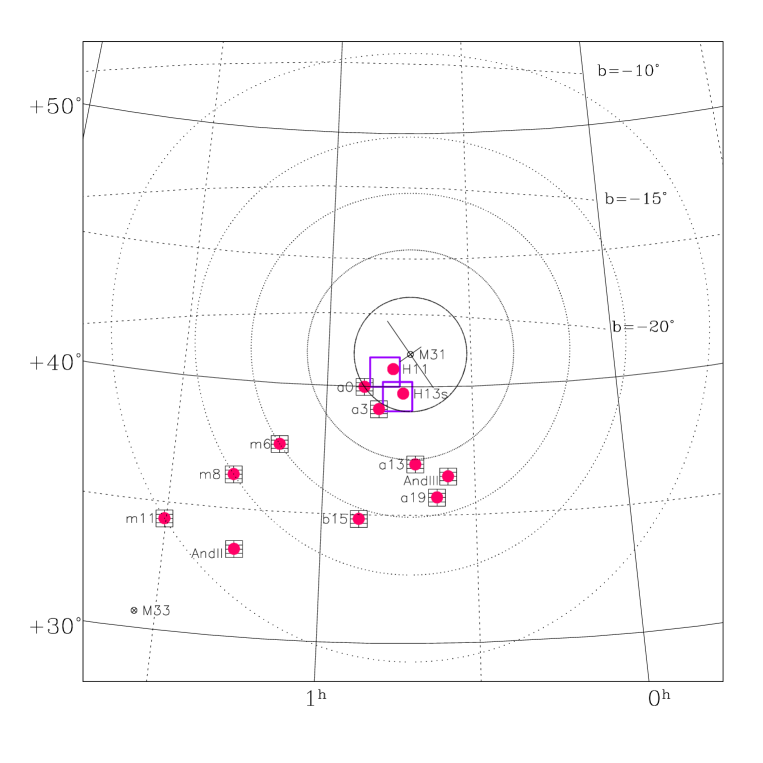
Figure 1.— Location of the fields used in this study relative to M31 (center). The size of M31’s visible disk, and orientation, is illustrated with two solid lines in the center. Lines of constant longitude and latitude are also shown. The smaller gridded squares represent schematically the field centers of the KPNO fields for which we have $DDO51$ photometry and the two larger squares indicate the approximate positions of the CFHT fields without $DDO51$ photometry. The filled circles show the approximate locations of the twelve fields for which we have Keck/DEIMOS spectroscopic observations.

Recently, a large number of ground and space based observations have targeted both the Milky Way and M31 to try to confirm these predictions directly. In this respect, M31 is often a better choice than our own Galaxy since we have a global, external view of it. The wealth of data collected to date has indeed confirmed certain theoretical predictions, while, at the same time, it has raised some new puzzles. For example, wide-field star-count maps of both galaxies have revealed abundant substructure in the halos of these systems, as predicted by simulations. In the Milky Way, the Sagittarius stream (Ibata et al., 1994; Majewski et al., 2003), the Magellanic stream (Mathewson, Cleary, & Murray, 1974) and the Monoceros stream (Yanny et al., 2003) present clear evidence that merging processes are prominent in massive galaxies and are still occuring today. Similarly, star-count maps of M31 (e.g., Ferguson et al., 2002; Ibata et al., 2005) have shown that its spheroid is very imhomogenous with many prominent density enhancements (e.g., the giant southern stream — Ibata et al., 2001).

The comparison of the Milky Way and M31 halo has also revealed several unanticipated results and notable differences between the two galaxies. Despite their similar overall size, the stellar density of M31’s spheroid appears to be 10$\times$ higher than that at a comparable location in the Milky Way (Reitzel, Guhathakurta, & Gould, 1998). Mould & Kristian (1986) surprisingly found that the “halo” of M31 at $R\sim$ 7 kpc is also 10$\times$ more metal rich than the Milky Way’s. This was also measured by Durrell, Harris, & Pritchet (1994) and by Rich, Mighell, & Neill (1996) over a larger radial distance, from $R$ = 5.3–19.4 kpc. Further studies of the metallicity distribution function (MDF) in M31 not only confirmed this result, but also showed that there is no evidence for an abundance gradient out to 30 kpc (Durrell, Harris, & Pritchet 2001, 2004, Bellazzini et al. 2003), a result at odds with model predictions. Differences between the Milky Way and M31 are also seen in the distribution of the ages of stars at large radii. The canonical picture of an old, metal-poor population simply does not appear to describe M31’s “halo”. Brown et al. (2003) used the Advanced Camera for Surveys (ACS) on the Hubble Space Telescope (HST) to target a minor-axis field at $R\sim 10$ kpc in M31 and produced a superb color-magnitude diagram (CMD) extending well below the main-sequence turnoff. Their data suggest a broad distribution of stellar ages in M31’s “halo”: over half the population of stars in this field have ages $\lesssim 11$ Gyr old. By mass, 30% of the stars are found to be 6–8 Gyr old. Rich et al. (2006, in preparation) have now obtained spectroscopy of stars in this HST field using the DEIMOS spectrograph on the Keck II telescope. We use these data below to confirm that the RGB population in the Brown et al. M31 “halo” field is much more metal rich than RGB stars in the Milky Way halo.

Until recently, there appeared to be another striking structural difference between the Milky Way and M31 spheroids. Whereas the Milky Way shows a de Vaucouleurs $R^{1/4}$ (de Vaucouleurs, 1958) surface brightness profile in the inner regions of the Galaxy and a power law $R^{-2}$ projected profile for the halo in the outer parts, Pritchet & van den Bergh (1994) found that the entire spheroid of M31 could be fit by a single $R^{1/4}$ profile. Their star-count measurements extended out to $R\sim$ 20 kpc along the south-east minor axis of M31, and demonstrated that the surface brighness profile of M31 falls off very steeply with increasing radius near the limit of their survey. Similarly, Durrell, Harris, & Pritchet (2004) found that an $R^{1/4}$ law is consistent with M31’s surface brightness profile out to 30 kpc.

Ostheimer (2003) carried out a survey that was a significant improvement over previous work in terms of both spatial coverage ($R\sim$ 10–165 kpc), photometric depth (1.5 mag arcsec^-2 fainter), and signal-to-background. His M31 surface brightness profile showed the first sign of a flattening (e.g., deviation of the slope from a de Vaucouleurs profile) in the outermost few bins ($>$80 kpc). By following up the Ostheimer (2003) imaging observations with multiobject Keck/DEIMOS spectroscopy, we have now been able to verify M31 red giant branch (RGB) member stars in each of the Ostheimer fields out to $R\sim$ 160 kpc. The spectroscopic data unequivocally show a break in the surface brightness profile of M31. In Guhathakurta et al. (2006a), we present the first detection of an $R^{-2}$ halo of stars in M31 extending out to a projected radius $>$160 kpc. Based solely on photometric data out to $R\sim$ 55 kpc, Irwin et al. (2005) also find a break in the surface brightness profile of M31 (although they claim that the outer component does not resemble a population II halo).

Following up on this discovery, this paper presents the first detection of a metallicity gradient in M31. Furthermore, we show that the crossover between the metal-rich and metal-poor components in our sample occurs at a minor-axis distance of $\sim$30 kpc, in excellent agreement with the transition radius that separates the newly discovered halo of M31 from the inner de Vaucouleurs ($R^{1/4}$) bulge. We propose that this new component is in fact the stellar halo of M31 (see also Chapman et al. 2006). Taken together, these results clarify that the actual structural disparities between the Milky Way and M31 may not lie in the properties of their halo populations, but rather in the relative sizes of the bulges of the two systems. The discovery of this metal-poor stellar halo also provides a powerful confirmation of galaxy formation models (see § 7.5).

Figure 2.— Sample M31 RGB spectra, one star from each of our twelve fields, as well as the spectrum of a typical foreground Milky Way dwarf star (bottom). The spectra have been corrected to zero velocity, normalized at $\rm\lambda\sim 8500\AA$, offset in $y$ arbitrarily, and smoothed using a 10 pixel ($\rm 3\AA$) boxcar function for illustration purposes only. The locations of the Ca ii triplet: 8498, 8542, and $\rm 8662\AA$ and pressure sensitive Na i doublet: 8183 and $\rm 8195\AA$ are indicated with arrows at the top of the figure. As expected, the Na i doublet is measured to be very strong in cool foreground Milky Way dwarf stars, but is absent in M31 RGB stars.

2. Observations and Data Reduction

The locations of the imaging/spectroscopic fields presented in this study are shown in Figure 1. The wide-field imaging observations were obtained with the Kitt Peak National Observatory (KPNO) 4-m telescope and Mosaic camera for most of our fields (Ostheimer, 2003). These are shown as gridded squares. The two larger open squares show the positions of very wide-field imaging observations obtained with the Canada-France-Hawaii 3.6-meter telescope and MegaCam camera. The filled circles indicate the positions of our twelve spectroscopic fields, all obtained with the Keck II telescope and DEIMOS instrument. The imaging for the outer fields was obtained by Ostheimer (2003) using the KPNO Mosaic camera, in the Washington System $M$ and $T_{2}$ bands and the intermediate-width $DDO51$ filter (Majewski et al., 2000). This filter allows measurement of the surface-gravity sensitive Mgb and MgH stellar absorption features and therefore provides a means to discriminate foreground Milky Way contaminants from M31 RGB stars. The innermost two fields in our study, H11 and H13s, are near enough to M31 that there is minimal foreground Milky Way dwarf contamination. We therefore did not observe these fields in the $DDO51$ filter. Rather, we obtained very wide-field Canada-France-Hawaii Telescope (CFHT) photometry in the $g^{\prime}$ and $i^{\prime}$ filters using the 1 degree² MegaCam camera. The $g^{\prime}$ and $i^{\prime}$ photometry was converted to Johnson-Cousins $V$ and $I$ using standard Landolt field observations.

Table 1

Date	Mask	Pointing center:		Field PA	No. Sci.
		$\alpha_{\rm J2000}$	$\delta_{\rm J2000}$	(∘E of N)	Targets
		(h:m:s)	(∘:′:′′)
2002 Aug 16	a3_1	00:48:21.16	+39:02:39.2	$+64.2$	85
2002 Aug 16	a0_1	00:51:51.32	+39:50:21.4	$-17.9$	89
2002 Oct 11	a3_2	00:47:47.24	+39:05:56.3	$+178.2$	80
2002 Oct 12	a0_2	00:51:29.59	+39:44:00.8	$+90.0$	89
2003 Sep 30	a13_1	00:42:58.34	+36:59:19.3	$+0.0$	80
2003 Sep 30	a13_2	00:41:28.27	+36:50:19.2	$+0.0$	71
2003 Sep 30	m11_1	01:29:34.44	+34:13:45.4	$+0.0$	72
2003 Oct 1	m11_2	01:29:34.35	+34:27:45.5	$+0.0$	68
2003 Oct 1	m6_1	01:09:51.75	+37:46:59.8	$+0.0$	75
2003 Oct 26	a3_3	00:48:23.17	+39:12:38.5	$+270.0$	83
2004 June 17	a0_3	00:51:50.46	+40:07:00.9	$+0.0$	90
2004 Sep 20	H11_1	00:46:21.02	+40:41:31.3	$+21.0$	139
2004 Sep 20	H11_2	00:46:21.02	+40:41:31.3	$-21.0$	138
2004 Sep 20	H13s_1	00:44:14.76	+39:44:18.2	$+21.0$	134
2004 Sep 20	H13s_2	00:44:14.76	+39:44:18.2	$-21.0$	138
2005 Jun 9	m6_2	01:08:36.22	+37:28:59.6	$+0.0$	72
2005 Jul 7	m8_1	01:18:11.56	+36:16:24.9	$+0.0$	56
2005 Jul 7	m8_2	01:18:35.87	+36:14:30.9	$+0.0$	59
2005 Jul 8	m11_3	01:30:01.53	+34:13:45.4	$+0.0$	80
2005 Jul 8	m11_4	01:30:37.33	+34:13:27.4	$+0.0$	75
2005 Aug 29	a19_1	00:38:16.05	+35:28:07.2	$-90.0$	71
2005 Sep 6	d2_1	01:17:07.46	+33:29:25.1	$-90.0$	139
2005 Sep 6	d2_2	01:16:43.29	+33:34:25.8	$+0.0$	141
2005 Sep 7	b15_1	00:53:23.63	+34:37:16.0	$-90.0$	65
2005 Sep 7	b15_3	00:53:37.77	+34:50:04.1	$-90.0$	74
2005 Sep 8	d3_1	00:36:03.83	+36:27:27.4	$+90.0$	120
2005 Sep 8	d3_2	00:35:39.61	+36:21:41.8	$+0.0$	122

Details on the imaging observations, slitmask design, spectroscopic observations, and data reduction of the fields a0, a3, a13, d3, a19, m6, b15, m8, d2, and m11 are given in § 2 of Gilbert et al. (2006) and Guhathakurta et al. (2006b). Similar information for the two innermost fields H11 and H13s can be found in § 3 of Kalirai et al. (2006). Keck/DEIMOS spectroscopic observations were obtained in each of the above pointings as discussed in Gilbert et al. (2006) and Kalirai et al. (2006). We briefly summarize the information presented in these papers. We used the 1200 lines mm^-1 grating (dispersion = $\rm 0.33\AA$ pixel^-1), providing a spectral resolution of $\rm 1.3\AA$ (FWHM) for typical 0$\farcs$8 FWHM seeing. We targeted the brightest M31 RGB stars ($20.0<I_{0}<22.5$ – the brightest in this window may in fact be asymptotic giant branch stars) in the photometry and built masks in an iterative process that maximized the total number of slits selected for highest priority objects. These, in the case of the outer fields, were largely based on the position of the star in the CMD and the position in the ($M-DDO51$) versus ($M-T_{2}$) color-color diagram (e.g., Majewski et al. 2000; Palma et al. 2003). As mentioned earlier, the latter provides a preselection to ensure high probability RGB stars, which is especially important in the outer regions of M31 where true RGB stars have sparse density. For the inner fields, a combination of the magnitudes and a stellarity (star-like) limit based on the morphology of the sources from SExtractor (Bertin & Arnouts, 1996) was used to prepare the masks. In general, the high density of objects in the inner fields allowed us to target $\sim$150 targets on each mask. All of the spectra were inspected visually and assigned a quality control index based on the quality and number of absorption lines visible. As discussed in Kalirai et al. (2006), a significant number of the fainter targets yielded spectra that did not show any obvious features due to low signal-to-noise (S/N). We determine the velocities for all objects that contain at least two spectral features (at least one definite and one other marginal line) by cross-correlating the observed spectra with a large database of template stellar and emission- and absorption-line galaxy spectra. The mean S/N of these good spectra is $\sim$10 per pixel and the velocity uncertainty from the cross-correlation is empirically estimated to be $\sim$15 km s^-1. The mean magnitude for these stars (with S/N $\sim$ 10 per pixel) is $I_{0}\sim 21.2$.

After removing galaxies, the twelve fields (27 masks) in this study contain 1070 stars for which we obtained a reliable velocity. Figure 2 shows a single representative spectrum of an M31 RGB star from each of these fields. Table 1 presents a summary of the observations.

3. A Clean Sample of M31 RGB Stars

A fraction of the 1070 stars in our sample are in fact foreground Milky Way dwarfs. In order to measure the MDF in M31’s bulge and halo, we first need to isolate M31 RGB stars from this contamination. We have developed a sensitive technique that uses probability distribution functions (PDFs) calculated from a training set of known RGB and dwarf stars to provide this discriminant (Gilbert et al., 2006). Using five criteria — (1) radial velocity, (2) intermediate-width $DDO51$ photometry, (3) Na i equivalent width (surface gravity sensitive), (4) position in the CMD, and (5) comparison between photometric and spectroscopic [Fe/H] estimates — each star in our sample is assigned five likelihood values of being a giant or a dwarf based on its location within each diagnostic plot. The individual probabilities are then combined to yield the final discriminant of whether the star is truly an M31 RGB star. In Figure 3 we show the properties of confirmed M31 RGB stars in six of our outer spectroscopic fields, a13, a19, m6, b15, m8, and m11. We have plotted four of the five diagnostics used to distinguish RGB stars from dwarfs, and have also overlayed empirical PDFs derived from the training set of definite RGB (solid darker curve) and dwarf (dashed/thin curve) stars. It is clear that the outer RGB stars predominantly agree with the RGB training set in all of their properties.

Figure 3.— Properties of confirmed M31 RGB stars in six of our outer spectroscopic fields (a13, a19, m6, b15, m8, and m11 - all located at $R>$ 60 kpc). Four of the five diagnostics used to distinguish RGB stars from foreground Galactic dwarf star contaminants are illustrated. (a) Radial velocity distribution of M31 RGB stars and dwarf stars [shaded-bold and dot-dashed histograms, respectively], compared to empirical probability distribution functions (PDFs) derived from training sets consisting of definite RGB and dwarf stars in all of our fields (solid and dashed curves, respectively). (b) Same as (a) for the $DDO51$ parameter, which is based on the star’s location in ($M-DDO51$) vs. ($M-T_{2}$) color-color space. For both (a) and (b), we have scaled back the dwarf star histograms by a factor of three for clarity and arbitrarily scaled the training set PDFs. (c) Equivalent width of the Na i $\rm 8190\AA$ absorption band versus de-reddened ($V-I$)₀ color for the RGB and dwarf stars [bold circles and crosses, respectively]. Bold and thin contours show 10%, 50%, and 90% enclosed fractions for RGB and dwarf star PDFs, respectively. (d) Same as (c) for the photometric metallicity estimate (CMD based, see § 5.1) versus spectroscopic metallicity estimate (based on the strength of the $\rm 8500\AA$ Ca ii triplet, see § 5.2). The dot-dashed diagonal line shows the one-to-one relation, which is followed nicely by confirmed RGB stars. It is reassuring that the M31 RGB distribution generally follows the RGB PDF and not the dwarf PDF.

A detailed discussion of the procedure used to average the individual PDFs into a likelihood distribution is given in Gilbert et al. (2006). In Figure 4 we present the final distribution of weighted average likelihoods, $\langle$$L_{i}$$\rangle$. Although any star with $\langle$$L_{i}$$\rangle$ $>$ 0 is a preferred M31 RGB star (whereas stars with $\langle$$L_{i}$$\rangle$ $<$ 0 are likely to be Milky Way dwarfs), we only select stars with $\langle$$L_{i}$$\rangle$ $>$ 0.5 for our clean M31 RGB sample. This ensures that the star is three times more likely to be an M31 RGB member than a Milky Way dwarf (see Gilbert et al. 2006). We also impose a strict cut to eliminate a few very blue stars that are inconsistent with the color of M31’s RGB (see Gilbert et al. 2006). The remaining sample (530 stars) are shown as shaded histograms in Figure 4. We stress that although it may not be clear from any individual diagnostic whether or not a star is a dwarf or a giant, the combination of the ten PDFs presents an unambiguous answer.

Table 2

Mask	$R$	No. Sci.	No. M31 RGB	No. Milky Way	No. M31 RGB	Comments
	(kpc)	Targets	Stars	Dwarfs	Spheroid Stars
H11	12	277	106	18	106
H13s	21	272	104	20	21	giant southern stream field
a0	30	268	67	30	67
a3	33	248	68	12	20	giant southern stream field
a13	60	151	18	23	18
d3	69	242	60	89	6	And III dwarf spheroidal field
a19	81	71	4	23	4
m6	87	147	9	49	9
b15	95	139	6	25	6
m8	121	115	1	24	1
d2	145	280	84	38	0	And II dwarf spheroidal field
m11	165	295	3	82	3

Figure 4.— The weighted average likelihood distinguishing M31 RGB stars ($\langle$$L_{i}$$\rangle$ $>$ 0.5 – shaded) from Milky Way dwarfs for each of our twelve fields. The fields are arranged in order of increasing projected distance from M31.

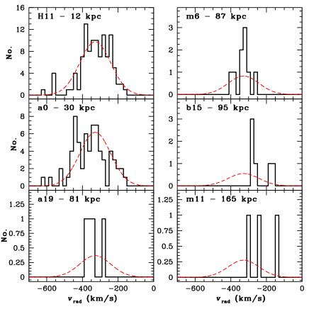
Figure 5.— Radial velocity histograms for confirmed M31 RGB stars in six representative bulge and halo fields, arranged in order of increasing distance from M31. A scaled Gaussian with the characteristic velocity and dispersion of our most populous field, H11, has been overlain on the data to show that the distribution of stars in each of these fields is roughly consistent with a broad Gaussian centered near M31’s systemic velocity.

As a point of interest, we note that some other studies of M31 have isolated Milky Way dwarfs from M31 RGB stars based solely on a velocity cut. Using our PDFs for the two minor axis fields H11 and a0, we calculate that such a cut will introduce a significant amount of Milky Way dwarf star contamination into the putative RGB sample. For example, invoking only a velocity cut of $v_{\rm rad}<$ $\rm-$100 km s^-1 to isolate M31 RGB stars from Milky Way dwarfs will lead to a contamination fraction of $\sim$15% in our data. Similarly, for a velocity cut of $v_{\rm rad}<$ $\rm-$150 km s^-1 cut, over 10% of all classified M31 RGB stars would actually be Milky Way dwarfs. For fields that sample the extended disk of M31 in the N-E or N-W quadrants, the contamination rates could be higher due to the rotation of M31’s disk which would cause the velocity histogram to overlap with the Milky Way dwarf distribution. This would of course be offset to some degree (perhaps completely) depending on the distance of these fields from M31’s center (i.e., the density of M31 RGB stars is much higher along the major axis).

In Table 2, we present the numbers of stars in each field that were determined to be secure M31 RGB stars and Milky Way dwarfs (measured using a $\langle$$L_{i}$$\rangle$ $>$ 0.5 cut) from the procedure outlined above. Further analysis from this point will involve only the cleaned M31 RGB sample.

4. Kinematics of Sample

In this section we briefly present kinematics of M31 RGB stars in some of our fields and demonstrate that the data are consistent with a broad Gaussian centered at M31’s systemic velocity. As can be seen from Figure 1, five of our pointings are located on the minor axis (H11, a0, m6, m8, and m11), two of the pointings are located on the giant southern stream (H13s and a3), and five pointings are removed from the minor axis (a13, d3, a19, b15, and d2). The data for the minor axis fields and the off axis pointings are likely fair representations of the bulge and halo of M31 (see § 6.1). However, the targeted stars in the giant southern stream (H13s and a3) and dwarf satellites (d2–And II and d3–And III) have very different kinematics than hot bulge or halo stars. As demonstrated in Ibata et al. (2004), Guhathakurta et al. (2006b), and Kalirai et al. (2006), the stream consists of a kinematically cold population of stars blueshifted relative to M31 (in H13s stream stars have $v_{\rm rad}<$ $\rm-$380 km s^-1, in a3 stream stars have $v_{\rm rad}<$ $\rm-$400 km s^-1). The stream is well removed, both azimuthally and radially, from all of our other pointings and does not contaminate these fields. Similarly, d2 and d3 are dominated by stars belonging to the two dwarf satellites And II ($\rm-$230 km s^-1 $<v_{\rm rad}<$ $\rm-$150 km s^-1) and And III ($\rm-$390 km s^-1 $<v_{\rm rad}<$ $\rm-$325 km s^-1). For each of these four fields we easily remove the contribution of the stream and satellite galaxies by making these velocity cuts, leaving a pure M31 RGB bulge and halo sample.

Figure 5 presents the velocity histograms for six fields in M31 that are not contaminated by the giant southern stream or one of the dwarf satellites. Velocity histograms for the giant southern stream can be found in Kalirai et al. (2006) (H13s) and Guhathakurta et al. (2006b) (a3). The fields shown here have been randomly chosen and sample the entire distance range over which we measure M31 RGB stars. The two minor axis fields with a large sample of stars, H11 and a0, clearly demonstrate that the majority of these stars form a broad, hot component centered near M31’s systemic velocity. For our most populated field (H11), we find $v_{\rm rad}\sim$ $\rm-$330 km s^-1 with a dispersion of $\sigma_{v}\sim 90$ km s^-1 (skew = 1.3). The velocity histograms for our outermost fields are affected by small number statistics. However, almost all confirmed M31 RGB stars in these fields (e.g., a19, m6, b15, and m11) have kinematics consistent with M31’s systemic velocity, $v_{\rm rad}\sim$ $\rm-$300 km s^-1. To demonstrate this, we have overlaid a scaled Gaussian with the mean and dispersion of the H11 field in each of these panels (dashed curve).

The combination of Figures 4 and 5 shows that we have detected a population of RGB stars belonging to M31’s bulge and halo in eleven of our twelve fields (the exception being field d2, which is dominated by stars belonging to M31’s dwarf satellite, And II). The final starcounts for these populations, in each field, are given in column 6 of Table 2 (this is the number after eliminating foreground dwarfs, M31 stream, and M31 satellite galaxy stars). Adding up all of the data, our sample consists of 261 bona fide M31 RGB bulge and halo stars, 47 of which have $R>$ 60 kpc. We stress that prior to this work, very few (if any) M31 halo RGB stars have been spectroscopically confirmed at these large radii.

5. Metallicity Measurements

We determine the metallicities of stars in our sample using two independent techniques, photometrically from the ($I$, $V{\rm-}I$) CMD and spectroscopically from the Ca ii triplet ($\rm\lambda\sim 8500\AA$).

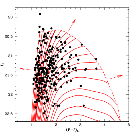
Figure 6.— CMD of all M31 RGB bulge and halo stars. Most stars are confined within a grid of theoretical isochrones (Vandenberg, Bergbusch, & Dowler, 2005) of age 12 Gyr spanning the metallicity range, [Fe/H] = $\rm-$2.31 to $+$0.49 (bold isochrone: [Fe/H] = $\rm-$1.0). A few outliers are found above the tip of the RGB (dashed line). The arrows indicate the direction in which we extrapolated metallicity measurements for a few stars. Section 5.1 discusses the determination of these metallicities for this sample.

5.1. Photometric Metallicity Determination

In Figure 6 we present the CMD for our entire M31 RGB bulge and halo sample. For this purpose, we first converted the Washington System ($M$, $T_{2}$) photometry into Johnson-Cousins ($I$, $V{\rm-}I$) magnitudes using the relations in Majewski et al. (2000). The systematic error in the slope of the color conversion from these relations is less than 3.6%, as measured by Majewski et al. (2000). Also shown are several theoretical isochrones ranging in metallicity from [Fe/H] = $\rm-$2.31 – $+$0.49, all with an age of 12 Gyr and [$\alpha$/Fe] = 0.0 (Vandenberg, Bergbusch, & Dowler, 2005). These have been adjusted to a distance of 783 kpc ($(m-M)_{0}=24.47$). Most of our sample is indeed confined within the bounds of the most metal-rich and metal-poor isochrones on the CMD. For reference, the bolder isochrone has a metallicity of [Fe/H] = $\rm-$1.0. The dashed line at the top of the isochrones indicates the tip of the RGB.

We compute photometric metallicities ([Fe/H]_phot) for these stars by first measuring the length in the CMD of a segment that extends from the most metal-poor isochrone to the most metal-rich. This is done at 35 points along the set of isochrones, extending from the base of our RGB sample in Figure 6 to well above the tip of the RGB (by linearly extrapolating the isochrones in brightness and color). The dashed curve on Figure 6 represents one of these length segments. We then normalize these 35 segments by their total length, hence computing an index, $X$, equal to the fractional distance that a point is away from the most metal-poor isochrone. This $X$ parameter is now a smooth function of metallicity, for a given $Y$ range, the distance above the base of the RGB in our sample (extending from 0 at the base to 1 at the tip of the RBG). Photometric metallicities are derived by measuring each star’s $X$ position and interpolating that within the relation that is appropriate given its $Y$ value. Although we do this for many $Y$ ranges (bins of size 0.1), we find that the $X$ versus [Fe/H] relations are not very sensitive to this parameter and vary smoothly and slowly over the entire magnitude range of RGB stars in our sample. Metallicities for confirmed RGB stars that lie outside the range of the isochrones are derived by extrapolating the $X$ versus [Fe/H] relations. As the CMD in Figure 6 shows, this mild extrapolation was required for only a few stars.

We also tested our [Fe/H]_phot measurements derived above using two independent sets of isochrones. Interpolating metallicities within a grid of the Padova models (Girardi et al., 2002) and the Yale-Yonsei models (Y² - Demarque et al. 2004) give consistent values to those derived using the Vandenberg, Bergbusch, & Dowler (2005) models. For a typical star, the mean [Fe/H] varies by less than 0.15 dex depending on which isochrone set is adopted. We find that the Padova models systematically yield slightly more metal-rich values than both the Vandenberg, Bergbusch, & Dowler (2005) and Demarque et al. (2004) models. We choose to adopt the Vandenberg, Bergbusch, & Dowler (2005) models as they also provide a grid of $\alpha$-enhanced isochrones over a broad metallicity range (see § 6.2).

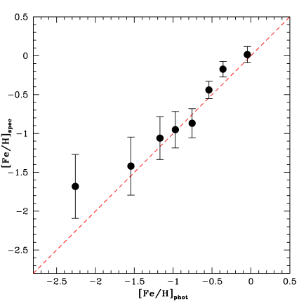
Figure 7.— Comparison of spectroscopic ([Fe/H]_spec) versus photometric ([Fe/H]_phot) metallicities of all M31 RGB bulge and halo stars. We have used a minimum bin size of 0.2 dex in [Fe/H]_phot to bin the sample, while ensuring a minimum of 20 stars in each bin. The data span a wide metallicity range and the two independently measured quantities are found to be in good agreement with one another over most of this range. For reference, a 1:1 relation is shown as a dashed line.

5.2. Spectroscopic Metallicity Determination

Independent of the method discussed above, we also determine metallicities for all of our M31 RGB bulge and halo stars using their spectra. This procedure relies on measuring the equivalent widths of the three Ca ii absorption lines (see Figure 2). The strengths of each of these lines are combined to yield a reduced equivalent width according to the prescription described in Rutledge, Hesser, & Stetson (1997). This reduced equivalent width is then calibrated empirically based on Galactic globular cluster RGB stars to yield [Fe/H]_spec (Rutledge et al., 1997). Further details on this procedure are given in Gilbert et al. (2006) and Guhathakurta et al. (2006b).

In Figure 7, we present a comparison of the two independently determined metallicity measurements for our sample. Given the larger scatter in [Fe/H]_spec, we have binned our sample by using a minimum bin size of 0.2 dex in [Fe/H]_phot while ensuring $>$20 stars in each bin. The individual [Fe/H]_phot and binned [Fe/H]_spec measurements are found to be in good agreement with one another over most of the metallicity range (1:1 line is shown), indicating that there are no systematic variations in our metallicity scales. This agrees with the results of Reitzel & Guhathakurta (2002) who also find a nice agreement between photometric and spectroscopic [Fe/H] measurements for RGB stars.

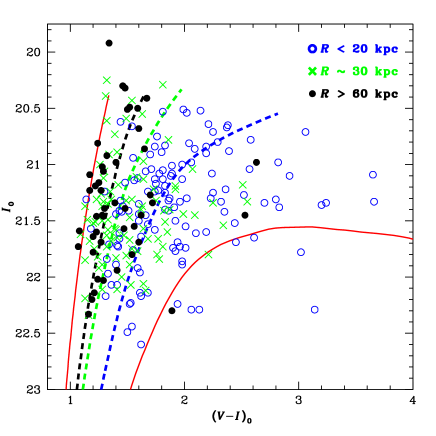
Figure 8.— The distribution of M31 RGB stars in the bulge ($R<$ 20 kpc, open circles), crossover region ($R\sim$ 30 kpc, crosses), and halo ($R>$ 60 kpc, filled circles) on the CMD show differences. In § 6.2, we provide evidence that these differences are related to the MDF of stars in M31’s different structural components. Solid curves represent theoretical isochrones (Vandenberg, Bergbusch, & Dowler, 2005) with [Fe/H] = $\rm-$2.31 (left) and 0.0 (right). The dashed curves are discussed in § 6.2.

We also note here that most classes of systematic biases/errors in our measurement of [Fe/H]_phot and [Fe/H]_spec (e.g., age errors, systematic errors in the models, etc.) will tend to affect different fields similarly. Therefore, although the absolute [Fe/H]_phot for any given star may have a large error (e.g., due to photometric calibration or incorrect distance modulus), the relative comparison of [Fe/H]_phot between different fields within our sample is more accurate. In § 7.1 we discuss several possible biases.

Figure 9.— Normalized MDFs of confirmed M31 RGB bulge and halo stars in each of our twelve fields. A general trend indicating the presence of metal-poor stars in the halo of M31 is seen. As a guide, the dotted line is fixed at [Fe/H] = $\rm-$1.0 in all panels. An arrow is indicated in the panel for m8 as we have re-normalized the MDF for this field. The cumulative distributions corresponding to these twelve fields are shown in Figure 10. In Figure 11 we bin all of the halo data ($R>$ 60 kpc) together to produce a more statistically significant sample from which we measure the mean metallicity and dispersion of M31’s halo. Note: field d2 does not contain any M31 RGB stars that are not members of And II.

6. Analysis

6.1. The Bulge and Halo Samples

As Table 2 shows, our M31 coverage ranges from a field located at $R$ = 12 kpc (H11) to a field located at $R$ = 165 kpc (m11). Given this very large range in radius from M31’s center, and our small number statistics in the outermost fields, we separate our fields into three broad regions. We define the bulge sample to be that represented by the H11 and H13s fields, the crossover region by the a0 and a3 fields, and the halo by the a13, d3, a19, m6, b15, m8, d2, and m11 fields (d2 containing no halo members). This separation is justified naturally for several reasons. First, as discussed in § 1, several authors have shown that there is no observed metallicity gradient in M31 out to $R\sim$ 30 kpc (e.g., Durrell, Harris, & Pritchet, 2004). One study, Irwin et al. (2006), suggests that there is no metallicity gradient out to $\sim$45 kpc. Second, Guhathakurta et al. (2006a) and Irwin et al. (2005) have recently shown that a power-law $R^{-2}$ profile dominates beyond this radius whereas a de Vaucouleurs $R^{1/4}$ surface brightness describes regions interior to this radius. Guhathakurta et al. (2006a) further demonstrate that the crossover of M31’s bulge and halo occurs near this radius. Therefore, $R\sim$ 30 kpc is a natural choice for separating the inner and outer samples. In addition to the two fields located near this intermediate radius (a0 and a3), two of our best sampled fields are located interior to this radius (H11 and H13s) while the remaining fields are located beyond this radius.

6.1.1 Color-Magnitude Diagrams

Figure 8 illustrates the CMD for M31 RGB stars in each of the three broad radial bins defined above. Also shown are two theoretical isochrones (solid curves - Vandenberg, Bergbusch, & Dowler 2005) with [Fe/H] = $\rm-$2.31 (left) and [Fe/H] = 0.0 (right). As we showed in Figure 6, the distribution of M31 RGB stars nicely follows the shapes of the isochrones. However, we can now see that some clear differences exist between stars belonging to the inner ($R<$ 20 kpc, open circles), crossover ($R\sim$ 30 kpc, crosses), and outer ($R>$ 60 kpc, filled circles) regions of M31. We show quantitatively below that the M31 RGBs in each of these regions are significantly different and that these differences relate to the MDF of each population. The dashed curves will be discussed later.

Figure 10.— Cumulative distributions of [Fe/H]_phot for M31 RGB bulge and halo stars in each of our twelve fields (solid curves). The dashed curves represent fixed Gaussians with [Fe/H]_phot = $\rm-$1.3 and $\rm-$0.4 to be used as guides. The same trend seen in the discrete distributions in Figure 9 is confirmed here. The outer fields are dominated by more metal-poor stars relative to the inner fields. Note: field d2 does not contain any M31 RGB stars that are not members of And II.

6.2. Metallicity Distribution Function and Radial Trends

Before presenting our MDFs for confirmed M31 RGB stars in each of the inner, crossover, and outer regions defined above, we construct MDFs for each of our twelve fields independently. These are shown in Figure 9 along with a fixed guide at [Fe/H] = $\rm-$1.0 (dotted line). The innermost fields, H11 and H13s, contain mostly stars with intermediate/metal-rich compositions. The a0 and a3 fields at $R\sim$ 30 kpc are dominated by a much broader MDF that extends to more metal-poor stars while still containing a metal-rich component. This MDF nicely supports the finding in Guhathakurta et al. (2006a) that a roughly equal mix of bulge (metal rich) and halo (metal poor) M31 stars reside at $R\sim$ 30 kpc (see § 7.2). Although individually affected by small number statistics, the outermost fields (second and third rows) in our study are dominated by a large number of metal-poor stars ([Fe/H]_phot $<\rm-$1). Directly comparing these fields to the inner fields, H11 and H13s shows a very obvious metallicity gradient in M31. Less than $\sim$4% of all stars in the two inner fields ($R<$ 21 kpc) combined have ([Fe/H]_phot $\leq\rm-$1) whereas almost 65% of stars in the outer fields ($R>$ 60 kpc) are this metal poor. Ostheimer (2003) found evidence for similar shifts in the proportions of metal rich and metal poor stars as a function of radius from a purely photometric analysis of all giant star candidates in these same fields.

In Figure 10 we present cumulative [Fe/H]_phot distributions for each of the twelve fields. The distributions confirm the conclusions drawn above. The outermost halo fields contain metal-deficient stars relative to the inner fields. As a guide, we have also shown two Gaussian distributions with means at [Fe/H]_phot = $\rm-$1.3 and $\rm-$0.4 and $\sigma$ = 0.4 (dashed curves).

In Figure 11 we present both the MDFs (top) and the cumulative Gaussians (bottom) for the bulge (H11 and H13s), crossover region (a0 and a3), and the halo (a13, d3, a19, m6, b15, m8, d2, and m11) of M31. All histograms have been normalized to unity for clarity. These data clearly show that we have indeed detected a metallicity gradient in M31. For $R<$ 20 kpc, we find $\rm\langle[Fe/H]_{\rm phot}\rangle=-0.47\pm 0.03$ ($\sigma$ = 0.39), for $R\sim$ 30 kpc we find $\rm\langle[Fe/H]_{\rm phot}\rangle=-0.94\pm 0.06$ ($\sigma$ = 0.60), and for $R>$ 60 kpc, we find $\rm\langle[Fe/H]_{\rm phot}\rangle=-1.26\pm 0.10$ ($\sigma$ = 0.72). Gaussian models with the mean and dispersion of the stars comprising the MDF in each of these groups are overlaid on the differential histograms as dashed curves. For completeness, we note that our spectroscopic metallicity for the outer halo ($\rm\langle[Fe/H]_{\rm spec}\rangle=-1.24\pm 0.12$, $\sigma$ = 0.85) is in excellent agreement with the measured photometric metallicity.

The CMDs for stars belonging to each of these three regions were presented in Figure 8. To illustrate the differences in the three CMDs, we have overlain isochrones in each panel of Figure 8 with the approximate mean metallicity of the respective population as determined above (dashed curves).

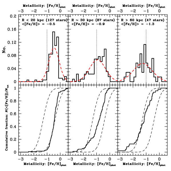
Figure 11.— (Top)—Normalized MDFs for each of the bulge (H11 and H13s), crossover region (a0 and a3), and halo (a13, d3, a19, m6, b15, m8, d2, and m11) regions. The dashed curves represent Gaussians with parameters fixed to the measured mean and dispersion of each MDF. The vertical dotted line is held fixed at [Fe/H] = $\rm-$1.0 to guide the eye.    (Bottom)—Cumulative distributions, corresponding to the above panels. The dashed curves represent fixed Gaussians with mean [Fe/H] = $\rm-$1.3 and $\rm-$0.4 ($\sigma$ = 0.4). The data unequivocally show a metallicity gradient in M31.

The photometric metallicities given above have been derived assuming isochrones with [$\alpha$/Fe] = 0.0. If we assume that M31’s halo is $\alpha$-enhanced, with [$\alpha$/Fe] = $+$0.3, the mean metallicity of the outer halo is found to be $\rm\langle[Fe/H]_{\rm phot}\rangle=-1.48\pm 0.11$ ($\sigma$ = 0.73).

6.3. Kolmogorov-Smirnov Tests

To test whether or not the MDFs of the inner, crossover, and outer regions of M31 (as defined above) truly differ significantly from one another, we have applied the two-sided Kolmogorov-Smirnov (K-S) test (Press et al., 1992). The K-S test makes no assumption about the distribution of the data and is therefore insensitive to possible spurious biases from arbitrary binning of data. The test looks at the cumulative fraction of each histogram and returns a statistic, $D$, which measures the maximum vertical deviation between the two curves. This statistic yields a significance level probability, $P$, that the null hypothesis (i.e., that the two data sets are drawn from the same distribution) is true. Therefore, small values of $P$ show that the two MDFs are significantly different whereas larger values (e.g., $\gtrsim$0.1) indicate that the two MDFs may have been drawn from the same distribution.

We find that the $R<$ 20 kpc inner M31 MDF is significantly different from the $R\sim$ 30 kpc MDF, yielding a tiny probability $P$ = 9.9$\times$10^-8 of the two being drawn from the same parent distribution. We also find that the $R\sim$ 30 kpc MDF is significantly different from the halo MDF, $R>$ 60 kpc. For this, the two-sided K-S test returns a probability of $P$ = 7.5$\times$10^-3. Additional tests confirm that the a0 and a3 MDFs that have been combined to form the $R\sim$ 30 kpc population are likely drawn from the same distribution, $P$ = 0.23 (at least it can not be shown that they are drawn from different distributions). Directly comparing the inner fields, H11 and H13s, with any of the outer fields a13, d3, a19, m6, b15, m8, or m11 shows them to be significantly different. Therefore, the K-S tests confirm our earlier conclusion that we have detected a metallicity gradient in M31.

In Figure 12 we present the radial metallicity distribution for M31. The mean photometric metallicity in each of our fields is plotted as a function of radius (open circles). The mean metallicity of the combined data for the inner, crossover, and outer regions is also plotted as larger filled circles. The data clearly show a trend of decreasing metallicity as the distance from M31 increases. For comparison, we also show the mean spectroscopic metallicity in each of our inner, crossover, and outer samples as filled squares. These measurements confirm that M31’s outer halo is dominated by stars much more metal-poor than the bulge. Table 3 summarizes our final MDF results.

Table 3

Field	$\langle{R}\rangle$	No. M31 RGB	$\rm\langle[Fe/H]_{\rm phot}\rangle$	$\sigma$
	(kpc)	Spheroid Stars
Bulge	14 (12–21)	127	$\rm-$0.47$\pm$0.03 ($\rm-$0.57$\pm$0.04)	0.39 (0.43)
Crossover	31 (30–33)	87	$\rm-$0.94$\pm$0.06 ($\rm-$1.12$\pm$0.07)	0.60 (0.68)
Halo	81 (60–165)	47	$\rm-$1.26$\pm$0.10 ($\rm-$1.48$\pm$0.11)	0.72 (0.73)

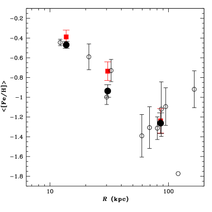
Figure 12.— The mean metallicity of M31 RGB stars in each of our fields as a function of increasing radius (open circles). The error bar on the most metal-poor data point, from the m8 field, has been omitted as it is based on only one stars and therefore is not reliable. The mean metallicity in the three coarser bins representing the inner, crossover, and outer regions of M31 are shown as larger filled circles. Spectroscopic metallicity measurements for these three components are shown as filled squares (the most metal-poor point strongly overlaps the photometric metallicity point). The data clearly shows that the halo of M31 is more metal-poor than the inner regions.

7. Discussion

7.1. Systematic Errors and Measurement Biases

As discussed in § 1, the detection of a radial metallicity gradient in M31 can directly constrain the global nature of chemical enrichment during the galaxy formation process. Our finding, however, is in contrast to previous observational work on M31 which has found no significant radial [Fe/H] gradient within $R<30$ kpc (e.g., Durrell et al. 2001, 2004). Even the recent Irwin et al. (2005) photometric survey found no significant color gradient for M31 RGB candidates out to $R\sim 55$ kpc, but uncertainties in statistical background subtraction make it difficult to interpret the significance of this null result. Given the relevance of a metallicity gradient and the apparent discrepancy with earlier studies, we now address and quantify some potential biases in our study. Understanding these effects is crucial to determining whether or not a spurious metallicity gradient could have been produced by our target selection and/or analysis procedure.

The target selection for the two innermost fields, H11 and H13s, is different from the outer fields in the sense that $DDO51$ filter pre-selection was not used. Although any selection effect from this may alter the overall shape of the [Fe/H] distribution, there should not be any relative bias among different $DDO51$-selected fields or, for that matter, among non-$DDO51$-selected fields. To investigate further whether a global bias exists between the inner and outer fields we can take advantage of the fact that two of our fields target the giant southern stream of M31. The target selection for one of these fields, H13s, does not involve $DDO51$ photometry, whereas for the other field, a3, it does. It is reassuring that both the Kalirai et al. (2006) study of H13s and the Guhathakurta et al. (2006b) study of a3 found a substantial population of high metallicity stars in the giant southern stream despite the $I<22.5$ magnitude cut used for spectroscopic target selection in both cases (see details below). A detailed comparison between these two fields can reveal whether $DDO51$ preselection biases the sample against the most metal-rich stars.

In Figure 13 we present the MDFs in H13s and a3, including only bona fide stream members. These have been selected by imposing velocity cuts on the data. In H13s, Kalirai et al. (2006) show that the stream consists of stars moving with $v_{\rm rad}\leq$ $\rm-$460 km s^-1. Similarly, Guhathakurta et al. (2006b) show that at the position of a3 stream stars have $v_{\rm rad}\leq$ $\rm-$425 km s^-1. There is some evidence for secondary velocity peaks in both of these data sets that may or may not be related to the stream, but we ignore these components here (see Kalirai et al. 2006 for further information). The resulting two MDFs are remarkably similar and show a strong peak of metal-rich stars with a small tail to metal-poor stars. For H13s, this MDF is well represented by a double Gaussian (shown as a dashed curve in the upper panel of Figure 13). We now superimpose this same model on the a3 data (dashed curve in lower panel), and find that the model that fits H13s needs to be adjusted only slightly by $\Delta$[Fe/H]_phot = $\rm+$0.1 dex to achieve the best fit of the stream MDF in a3: this was determined by fixing the relative spacing, standard deviations, and relative fraction of stars in the two components of the double Gaussian and only fitting for an overall offset. This shifted double Gaussian is shown as a dotted curve in the lower panel. The comparison of these two (differently selected) stream samples shows that any systematic [Fe/H] offset between them is very small. Since there are several other sources of systematic errors in [Fe/H] at this level or greater, we ignore this 0.1 dex offset; in fact, this apparent [Fe/H] offset may well be a result of the fact that our a3 sample probes deeper down the RGB luminosity function than the H13s sample (see discussion below). We note that if we did apply this potential offset between $DDO51$-selected and non-$DDO51$-selected data, the radial metallicity gradient in M31 would become stronger.

We note that an intrinsic metallicity gradient in the giant southern stream is unlikely over such a small radial extent ($R=21$–33 kpc). Several investigations have shown that the stream is young and was produced less than an orbital period ago (e.g., $\lesssim 2$ Gyr—Ibata et al. 2004). The radial extent above represents a very small difference in dynamical age and it would be difficult for a metallicity gradient to have developed within this timeframe.

Several additional biases exist in our data that would tend to weaken an observed gradient compared to any true radially-outward decrease in the mean metallicity of M31:

• The tip of the RGB is fainter for more metal-rich populations (see Figure 6). Thus, our magnitude cut for spectroscopic target selection ($20<I_{0}<22.5$) can bias the sample against the inclusion of the most metal-rich RGB stars (Reitzel & Guhathakurta 2002). This bias, if present, is expected to be stronger for the bulge than for the halo. This is because our target selection procedure (see Guhathakurta et al. 2006b) includes somewhat fainter targets, on average, in the outer fields due to the sparseness of luminous M31 RGB stars in these regions.

• The same PDF (see § 3) is being used to separate M31 RGB stars from foreground Milky Way dwarfs in all fields. This selection would tend to pick out RGB stars from the same region of the [Fe/H]_phot (or location in the CMD or $V{\rm-}I$ color) space at all radii (see Gilbert et al. 2006 for details). Given that our RGB PDF is based on “training set” stars drawn mostly from the inner fields, these PDFs favor higher [Fe/H]_phot values. In fact, Figure 3 (d) clearly shows that the RGB training set PDF does not sample metal-poor stars very well. Therefore, the true radial trends in metallicity may be even larger than observed.

• We have assumed a constant age of 12 Gyr for all stars in M31. However, the Brown et al. (2003) study indicates that the bulge contains a substantial fraction of intermediate age stars. By contrast, one expects the halo population to be old by analogy with the Milky Way’s halo. If in fact the inner region of M31 probed in this study is younger on average than the halo, then our photometric metallicities have been underestimated (i.e., assigned to be more metal-poor than they truly are) in this region. In fact, the comparison between [Fe/H]_phot and [Fe/H]_spec in Figure 12 suggests this. Therefore the adoption of younger isochrones in the bulge would lead to higher metallicities for these stars and a larger metallicity gradient. A shift in age from 12 to 6 Gyr translates to a $+$0.3 dex offset in [Fe/H]_phot.

• We have assumed that all stars in M31 are not enhanced in their $\alpha$-element abundances, ([$\alpha$/Fe]). Stars in the Milky Way’s halo are known to be $\alpha$-enhanced ([$\alpha$/Fe] = $+$0.3) and it is generally believed that this is a result of the stars in the halos of galaxies forming in early “bursts”. If the M31 halo is also $\alpha$-enhanced, then our use of [$\alpha$/Fe] = 0 isochrones has overestimated the metallicity for stars in this component (i.e., assigned to be more metal-rich than they truly are). We determined earlier that the mean metallicity of our M31 RGB halo sample is in fact $\sim$0.2 dex more metal-poor if we assume [$\alpha$/Fe] = $+$0.3 (i.e., we calculate $\rm\langle[Fe/H]_{\rm phot}\rangle=-1.5$ for M31’s halo under this assumption).

These additional biases strengthen our detection of a metallicity gradient in M31 are suggest that, if anything, the detected gradient is likely smaller than the true gradient.

7.2. Bulge/Halo Ratio

The analysis presented in this paper suggests that, over a large range of radial distances (12–165 kpc), there is a metallicity gradient within M31. This brings up the question: Is this metallicity gradient intrinsic to the bulge and/or halo, or are we seeing two overlapping M31 structural components that are each homogenous but distinct from each other in terms of their chemical abundance properties? One way to test these two scenarios is to consider the crossover region at 30 kpc, where we find a mean metallicity of $\rm\langle[Fe/H]_{\rm phot}\rangle=-0.94\pm 0.06$. Guhathakurta et al. (2006a) showed that at this radius there is roughly an equal mix of bulge and halo stars based entirely on fits to the minor-axis surface brightness profile of M31. If our data are consistent with the latter scenario (e.g., a homogenous bulge and halo), then the 30 kpc MDF should in fact be an equal superposition of the distinct bulge and halo MDFs. To test this, we randomly selected 47 bulge stars and grouped them together with the same number of stars in the halo sample. The resulting composite MDF is compared to the 30 kpc MDF derived from the a0 and a3 fields and found to be very similar. A two-sided K-S test (see § 6.3) between this composite “bulge+halo” MDF and the 30 kpc MDF returns a probability of the null hypothesis being true of $P>$ 0.50 (i.e., of the two samples being drawn from the same parent population).

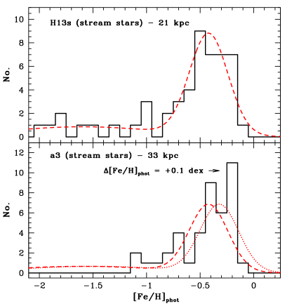
Figure 13.— MDFs for giant southern stream stars in H13s (top) and a3 (bottom). The two MDFs are found to be very similar. We find that the best fit double-Gaussian model to H13s (dashed curve) needs to be shifted only by $\Delta$[Fe/H]_phot = $\rm+$0.1 dex to fit the distribution of stars in the a3 field. This offset may result from a bias related to the way objects were selected in the inner and outer fields in our study (see § 7.1 for more information).

We therefore conclude that our data are consistent with a chemically homogenous bulge and halo whose relative contributions change systematically with radius and give rise to the observed metallicity gradient. This is not to say that M31’s bulge and halo are perfectly homogenous in a large-scale radial sense—only that our present samples lack the size and precision to detect any subtle metallicity gradients that may be intrinsic to the bulge or halo. For example, Figure 12 shows a very mild trend that an inverted metallicity gradient may be present in the halo of M31. However, splitting our 60–165 kpc halo fields into two bins (e.g., $R<$ 100 kpc and $R<$ 100 kpc) suggests that such a trend is statistically not significant (marginally). This measurement is difficult to make given the small number of stars. Future samples will no doubt be able to rectify this situation and allow us to characterize radial trends in the intrinsic chemical abundance properties of the bulge and halo in detail.

7.3. Relation of our Fields to M31’s Disk

None of the fields used in this study are contaminated by M31’s extended disk to any significant degree. Ibata et al. (2005) find that this disk is a low-surface brightess, kinematically cold (velocity dispersion, $\sim$30 km s^-1) structure at $R$ = 15–40 kpc and is an extention of the inner disk.

Our fields tend to lie close to M31’s minor axis, and are therefore well removed from the major axis. The most susceptible fields in our study that could potentially suffer from this contamination are the two innermost pointings, H11 and H13s. The projected distance of H13s is 21 kpc, which in the plane of the disk is $>$80 kpc. Therefore this field is located well beyond the extendend disk and Kalirai et al. (2006) have already ruled out any significant contribution to this field by a smooth disk population. We now focus on H11, which is located at $R$ = 12 kpc in the bulge of M31 (i.e., 50 kpc in the disk). We can rule out disk star contamination in this field based on several independent arguments,

• Guhathakurta et al. (2006a) present the surface brightness profile of M31 and show that at the position of H11, disk stars are expected to be greatly outnumbered by bulge stars. The bulge contribution to H11 is at least an order of magnitude greateer than the disk contribution.

• Figure 5 (Rich et al. 2006, in preparation) shows that the velocity histogram of H11 is well represented by a broad Gaussian centered near M31’s systemic velocity. There is no evidence for a 30 km s^-1 kinematically cold population (as seen in the fields that probe the extended disk of M31 in Ibata et al. 2005). In fact, the velocity dispersion of M31 RGB stars in H11 is measured to be approximately three times higher than that of M31’s extended disk. A maximum likelihood analysis of the H11 radial velocity data indicates that it is impossible to hide a substantial fraction of the stars in a kinematically cold (30 km s^-1) component (Reitzel et al. 2006, in preparation). Although this extended disk population dominates Ibata et al.’s RGB samples in fields near the major axis, their two minor axis fields, F05 and F07, also show no evidence of this population, as noted by the authors.

• Another scaling argument based on kinematics can be used to rule out the presence of a substantial fraction of M31 disk members in the H11 field. Figure 9 in Kalirai et al. (2006) shows radial velocity histograms for H11 ($R$ = 12 kpc, S-E minor-axis), H13s ($R$ = 21 kpc, giant southern stream), and H13d ($R$ = 25 kpc, N-E major-axis). Consistent with Ibata et al. (2005), our H13d field shows a kinematically cold population of stars, presumably M31’s disk. This field lies at 25 kpc in the disk plane, and also at 25 kpc in the bulge (as it is on the major axis). We find that two-thirds of the RGB stars in this field belong to the cold component (disk) and one-third are part of a dynamically-hot (bulge) component (Reitzel et al. 2006, in preparation). By comparison, our H11 field is located at 50 kpc in the disk plane and 20 kpc in the bulge (accounting for the 5:3 flattening of the bulge). Thus, the H11 field is twice as far out in the disk as H13d (ten versus five disk scale-lengths) and at a slightly smaller radial distance in the bulge. Moving out in the disk by five exponential scale lengths reduces the disk contribution by over two orders of magnitude. Thus, very few, if any, disk members should be present in our H11 field.

• T. Brown et al. (2006, in prep) have recently found evidence for younger stars in M31’s disk that are not seen in H11. By obtaining ultra-deep HST/ACS observations of stars in both of these fields (directly overlapping our pointings), Brown et al. are able to reach the main-sequence turnoff in M31’s bulge and disk. The reconstructed star formation histories of the these two components indicate some clear differences. For example, the disk field contains a younger main sequence and is generally more metal-rich than the bulge field. Therefore, these independent observations also suggest that our H11 field is not contaminated with disk stars and rather represents M31’s bulge.

Therefore, the surface brightness, kinematics, ages, and metallicities of stars in H11 argue against them being part of a disk like component in M31. We note that our next closest field, a0, is located at $Rsim$ 30 kpc in M31’s halo (i.e., over 130 kpc in the disk) and therefore does not sample the extended disk.

Worthey et al. (2005) make the radical hypothesis that a thick disk dominates the entire region within $R<$ 50 kpc in M31. This hypothesis was put forward to explain the high mean metallicity seen in previous studies of M31, but was not based on any kinematical data. Reitzel et al. (2006, in preparation) show that the stellar kinematics in the inner regions of M31 are inconsistent with Worthey et al.’s hypothesis, and confirm that the H11 and H13s samples used in this work represent M31’s bulge population instead.

7.4. Metallicity Distribution of the M31 Bulge: Comparisons to Other Studies

Although the halo sample of M31 RGB stars presented in this work is unique, a limited number of studies have probed the MDF of the bulge of M31 (although these studies have often referred to this component as the “halo”). The best study comes from ultra-deep HST/ACS observations by Brown et al. (2006) who have studied both the bulge and giant southern stream. These data reach faint enough to detect the lower RGB, horizontal branch, and main-sequence turnoff of M31. At these fainter magnitudes, there is minimal foreground dwarf star contamination. The HST CMDs of these two fields show striking similarities over all of the above phases of stellar evolution suggesting that the ages and metallicities of stars in the two fields are very similar. Furthermore, our H11 and H13s Keck/DEIMOS spectroscopic pointings have been carefully chosen to directly overlap these two HST/ACS fields. In Brown et al. (2003), it was shown that the H11 CMD contains both metal-poor and metal-rich stars ($\rm[Fe/H]>-0.5$). Given the striking similarity between the HST CMDs in these two fields, the H13s field must have a comparable MDF. Our measurement of the MDF in H11 and H13s confirm this (see Figure 10), both showing a distribution of stars near $\rm[Fe/H]\sim-0.5$.

The MDF of M31’s bulge has also been probed photometrically by Durrell, Harris, & Pritchet (2001) ($R\sim 20$ kpc) and Durrell, Harris, & Pritchet (2004) ($R\sim 30$ kpc). These measurements are based on wide field CFHT data. Durrell et al. compute the MDF by interpolating the location of stars on the CMD within a grid of $\alpha$-enhanced RGB models. This is done both for the target fields and for well-removed control fields. The final MDF is obtained by subtracting the control field MDF from the target field MDF. The results, in both fields, indicate that M31’s bulge is dominated by relatively high metallicity stars, $\rm\langle[m/H]\rangle\sim-0.5$ ($\rm\langle[Fe/H]\rangle=-0.8$, for [$\alpha$/Fe] = $\rm+$0.3). As Table 3 shows, our inner field is located interior to Durrell et al.’s 20 kpc pointing, and our crossover field is located slightly exterior to Durrell et al.’s 30 kpc pointing. Our measured metallicities, assuming the same [$\alpha$/Fe] = $\rm+$0.3 adopted by Durrell et al., are found to nicely bracket Durrell et al’s metallicity (see Table 3). This suggests that Durrell et al. have succeeded in statistically eliminating Milky Way dwarf stars with their use of an appropriate control field. Of course, this becomes more difficult as the distance from M31 increases, and therefore the methods discussed in Gilbert et al. (2006) become more important.

Other studies of M31 (e.g., Worthey et al. 2005, Bellazzini et al. 2003) have similarly concluded that the bulge is dominated by metal-rich stars ($\rm\langle[Fe/H]\rangle\sim-0.5$). Both these studies, and those discussed above, vary from one another in terms of both the source of the data and the types of models used to determine metallicity. Therefore, external comparisons of these results to our MDFs for H11 and H13s may not yield a perfect agreement and are not as powerful as relative comparisons of the MDF at various radii from a single data set (as presented in this paper). However, it is encouraging that such an external comparison does in fact yield similar metallicities and thus suggests that net effect of systematic errors in our MDFs is small.

7.5. The M31 Halo Versus the Milky Way Halo

In § 1 we discussed the assembly of massive galaxies such as the Milky Way and M31 in the context of hierarchical merging of smaller galaxies. Several predictions arise from this theoretical framework that have, until now, been challenged by our understanding of M31. Both structurally and in terms of chemical enrichment, the M31 “halo” was believed to be different from our own Galactic halo and different from the predictions of generally-accepted halo formation models. The wide-field imaging survey of Ostheimer (2003) was the first to find preliminary evidence of a metal-poor stellar halo in M31: it used $DDO51$ selection to greatly reduce foreground contamination by Milky Way dwarf stars and was thereby able to probe out to larger radii than previous studies. By coupling the Ostheimer $DDO51$ photometry with Keck/DEIMOS spectroscopy, Guhathakurta et al. (2006a) showed that M31 does possess a stellar component that is structurally distinct from its bulge and whose radial extent ($R>160$ kpc) and surface brightness profile ($\sim R^{-2}$) resemble those of our Galaxy’s stellar halo.

In this paper we have taken another step toward bridging the apparent disparity between M31 and the Galaxy/galaxy formation models by showing that this newly-discovered stellar halo in M31 is chemically distinct from its bulge, and is in fact quite metal poor: $\rm\langle[Fe/H]_{\rm phot}\rangle=-1.5\pm 0.1$ ($\sigma$ = 0.7). For comparison, Morrison et al. (2003) have recently measured metallicities from spectra of Milky Way halo RGB stars located at distances between 15 and 83 kpc from the Galactic center. The mean metallicity of this sample is measured to be $\rm\langle[Fe/H]\rangle=-1.6$ ($\sigma$ = 0.6), in good agreement with earlier studies. Therefore we find that the mean metallicity, and spread, of the M31 halo is similar to that of the Galactic halo.

The results presented in this paper show that a survey out to 20–30 kpc is not sufficient to properly isolate the M31 halo. In the Milky Way, the halo begins to dominate the thin disk at a radius interior to 10 kpc, locally (Majewski 1993). Therefore, our sampling distance in M31 is not comparable to the Milky Way. M31 likely contains a substantially larger bulge than the Milky Way and this bulge dominates over the halo in all previous studies of M31 that were limited to the central few degrees of the galaxy. Our data show clear evidence of a halo and bulge in M31 that are distinct from each other in terms of both structure and chemical abundance properties.

Prior to the detection of 47 M31 halo stars in this analysis, very few (if any) spectroscopically confirmed RGB stars had been detected in M31 with $R\gtrsim$ 60 kpc. Future observations will allow us to gather larger bulge and halo samples to establish whether or not these components contain intrinsic radial metallicity gradients. A detailed study of the true halo of M31 will require new observational strategies to gain significant insights into this important, but tenuous/elusive, stellar population.

8. Conclusions

Imaging and multiobject spectroscopic surveys of M31 have recently brought to light several unanticipated results. By isolating M31 RGB stars from Milky Way foreground dwarf contamination using a new technique, we are able to probe further into the outskirts of M31 than previous studies ($R$ = 12–165 kpc). In a separate paper we established the existence of a true stellar halo in M31, thereby resolving a long-standing concern that the surface brightness profile of M31 looks different from the Milky Way. In this paper, we analyze the metallicity distribution function of stars in twelve fields spanning this large radial extent. Our data show a radial metallicity gradient in the spheroid (bulge and halo) of M31. The outer region of M31 ($R>$ 60 kpc), dominated by its halo, is composed of stars deficient in metals relative to those in the inner region. Based on the sample of 47 stars, we find a mean chemical abundance of $\rm\langle[Fe/H]_{\rm phot}=-1.48\pm 0.11$ ($\sigma$ = 0.73) for the newly discovered halo of M31 (assuming [$\alpha$/Fe] = $+$0.3). This confirms predictions from current galaxy formation models which suggest that the inner regions of large galaxies should be chemically enriched relative to the outer regions.

References

- Bellazzini et al. (2003) Bellazzini, M., Cacciari, C., Federici, L., Fusi Pecci, F., & Rich, R. M. 2003, A&A, 405, 867
- Bertin & Arnouts (1996) Bertin, E., & Arnouts, S. 1996, A&AS, 117, 393
- Brook et al. (2004) Brook, C. B., Kawata, D., Gibson, B. K., & Flynn, C. 2004, MNRAS, 349, 52
- Brown et al. (2006) Brown, T. M., Smith, E., Guhathakurta, P., Rich, R. M., Ferguson, H. C., Renzini, A., Sweigart, A. V., & Kimble, R. A., 2006, ApJ, 636, L89
- Brown et al. (2003) Brown, T. M., Ferguson, H. C., Smith, E., Kimble, R. A., Sweigart, A. V., Renzini, A., Rich, R. M., & VandenBerg, D. 2003, ApJ, 592, L17
- Bullock & Johnston (2005) Bullock, J. S., & Johnston, K. V. 2005, ApJ, 635, 931
- Chapman et al. (2006) Chapman, S. C., Ibata, R., Lewis, G. F., Ferguson, A. M. N., Irwin, M., McConnachie, A., & Tanvir, N. 2006, ApJ, submitted (astro-ph/0602604)
- de Vaucouleurs (1958) de Vaucouleurs, G. 1958, ApJ, 128, 465
- Demarque et al. (2004) Demarque, P., Woo, J.-H., Kim, Y.-C., & Yi, S. K. 2004, ApJS, 155, 667
- Durrell, Harris, & Pritchet (1994) Durrell, P. R., Harris, W. E., & Pritchet, C. J. 1994, AJ, 108, 2114
- Durrell, Harris, & Pritchet (2001) Durrell, P. R., Harris, W. E., & Pritchet, C. J. 2001, AJ, 121, 2557
- Durrell, Harris, & Pritchet (2004) Durrell, P. R., Harris, W. E., & Pritchet, C. J. 2004, AJ, 128, 260
- Ferguson et al. (2002) Ferguson, A. M. N., Irwin, M. J., Ibata, R. A., Lewis, G. F., & Tanvir, N. R. 2002, AJ, 124, 1452
- Font et al. (2006) Font, A. S., Johnston, K. V., Bullock, J. S., & Robertson, B. E. 2006, ApJ, 638, 585
- Gilbert et al. (2006) Gilbert, K. M., Guhathakurta, P., Kalirai, J. S., Rich, R. M., Majewski, S. R., Ostheimer, J. C., Reitzel, D. B., Cenarro, A. J., Cooper, M. C., Luine, C., & Patterson, R. J. 2006, ApJ, submitted (astro-ph/0605171)
- Girardi et al. (2002) Girardi, L., Bertelli, G., Bressan, A., Chiosi, C., Groenewegen, M. A. T., Marigo, P., Salasnich, B., & Weiss, A. 2002, A&A, 391, 195