Parameter estimation of binary compact objects with LISA: Effects of time-delay interferometry, Doppler modulation, and frequency evolution

Abstract

We study the limits on how accurately LISA will be able to estimate the parameters of low-mass compact binaries, comprising white dwarfs (WDs), neutron stars (NSs) or black holes (BHs), while battling the amplitude, frequency, and phase modulations of their signals. These modulations will arise from LISA’s motion relative to the source, the evolution of the source emission frequency, and time-delay interferometry. We show that Doppler-phase modulation aids sky-position resolution in every direction, improving it especially for sources near the poles of the ecliptic coordinate system by a factor of at least six more than those near the ecliptic. However, the same modulation increases the frequency estimation error by a factor of over 1.5 at any sky position, and at a source frequency of 3 mHz, which is near the high-frequency end of the “unresolvable” white-dwarf confusion noise. Since accounting for Doppler-phase modulation is absolutely essential at all LISA frequencies and for all chirp masses in order to avoid a fractional loss of signal-to-noise ratio (SNR) of more than 30%, LISA science will be simultaneously aided and limited by it. For a source with an initial instantaneous frequency $\nu\lower 2.15277pt\hbox{$\;\buildrel>\over{\sim}\;$}2.5$ mHz, searching for its chirp or frequency evolution over a one-year duration worsens the error in the estimation of $\nu$ by a factor of over 3.5 relative to that of sources with $\nu\lower 2.15277pt\hbox{$\;\buildrel<\over{\sim}\;$}1$ mHz. Increasing the integration time to 2 years reduces this relative error factor to about 2, which still adversely affects the resolvability of the galactic binary confusion noise. Thus, unless the mission lifetime is increased several folds, the only other recourse available for reducing the errors is to exclude the chirp parameter from ones search templates. Doing so improves the SNR-normalized parameter estimates. This works for the lightest binaries since their SNR itself does not suffer from that exclusion. However, for binaries involving a neutron star, a black hole, or both, the SNR and, therefore, the parameter estimation, can take a significant hit, thus, severely affecting the ability to resolve such members in LISA’s confusion noise. Among the affected sources are galactic low-mass binaries containing a black hole, about which very little is known and which LISA may detect. Finally, we demonstrate how relative to a Michelson network a time-delay interferometric (TDI) data-combination network will have a different sensitivity sky-pattern and discuss its effect on parameter estimation.

I INTRODUCTION

The Laser Interferometric Space Antenna (LISA) is a proposed space-based broad-band gravitational wave (GW) detector funded by the National Aeronautics and Space Administration (NASA) and the European Space Agency (ESA) PrePhaseA . Unlike its extant and proposed earth-based counterparts, which include LIGO Abbott:2003vs , VIRGO VIRGO , TAMA TAMA , GEO Willke:2002bs , and LCGT Mio:2003ii , it enjoys guaranteed sources, specifically galactic binaries, such as AM CVn, HP Lib, WD 0957-666, RXJ1914+245, and 4U1820-30 Cutler:2002me ; Nayak:2003na . In fact, LISA will be so sensitive that the population of galactic binaries of compact objects, which comprise white dwarfs (WDs), neutron stars (NSs), and black holes (BHs), will create source confusion noise that towers over LISA’s instrumental noise near the sweet spot of its observation band Bender:1997hs ; hils ; nelemans . This can potentially affect the detection of other GW sources.

The confusion noise from WD binaries will be especially worse below about 3 mHz, where a good fraction of it, with low signal strengths, will be unresolvable. Galactic binaries that are bright enough or orbiting fast enough form a potentially resolvable population extending up to about 20 mHz. Our ability to resolve this latter class of sources will largely depend on how well we can estimate their signal parameters. Although the development of algorithms for resolving the component sources is still at its nascency gclean ; mohanty ; Crowder:2006wh , it is already clear that the smallness of the parameter errors is of utmost significance to the success of any of these algorithms. The focus of this paper is to study the role of different sources of these errors and determine the limits on how small we can keep them.

The problem of parameter-estimation accuracy has been studied for a variety of LISA sources in the past. Cutler did the first systematic study on this subject for monochromatic sources and super-massive black hole mergers Cutler:98 . Takahashi and Seto Takahashi:02 studied the problem exclusively in the context of low-mass compact binaries. They placed emphasis on the determination of the chirp parameter and its role in unraveling the distance to a binary, following an idea due to Schutz Schutz . Barack and Cutler Barack:2003fp studied this problem in the context of extreme-mass-ratio inspiraling binaries. Vecchio and Wickham Vecchio:2004ec extended earlier parameter estimation studies to beyond the long-wavelength approximation by including the frequency-dependent modulation of LISA’s beam-pattern functions arising at higher frequencies. They showed that invoking this approximation results in atmost a 3% loss in the SNR, but can have significant effects on the parameter accuracy (anywhere from 5% to a factor of 10) in the source frequency range 3mHz$\lower 2.15277pt\hbox{$\;\buildrel<\over{\sim}\;$}\nu\lower 2.15277pt\hbox{$\;\buildrel<\over{\sim}\;$}$10mHz.

All of these works, however, assumed that the data being filtered are two linearly independent LISA data streams, called Michelson variables, which measure the differential changes of length in LISA’s three arms. While these early works were instrumental in deriving useful lower-limits on the parameter errors of high signal-to-noise ratio (SNR) sources, the attainability of these limits is unclear because the Michelson variables will suffer from the presence of excess noise arising from the laser frequency fluctuations and optical bench motion. The first noise source alone is sufficient to ruin LISA’s characteristic strain sensitivity by several orders of magnitude. Fortunately, this critical problem has been addressed by devising a method for combining LISA’s data streams in software to produce data combinations that have these noises mitigated to the level of LISA’s noise budget Tinto:yr ; Armstrong:99 ; TEA . This method is termed as time-delay interferometry (TDI) and will be introduced in Sec. II.

In this work, like Takahashi and Seto, we consider the parameter estimation accuracy of low-mass compact binaries that are not necessarily monochromatic. But unlike that work, we base our accuracy limits on TDI variables and do not use the long-wavelength approximation. We study the role of the chirp-parameter, which is tantamount to a monotonic increase in the inspiral frequency, in affecting the accuracies of all signal parameters. We also quantify the effect of the Doppler-phase modulation to the same end. Our study shows in what regions of the parameter space the effects of searching for the chirp parameter or the effect of Doppler-phase modulation are not negligible. This can be useful in simplifying prototypical studies for those sources for which these effects are small. On the other hand, parameter regions where a search for the chirp in a signal can hurt the accuracy of the other parameters estimates are identified. Moreover, we demonstrate that the sensitivity sky-pattern of a network of TDI variables is very different from that of a network of Michelson variables. A similar difference exists in parameter accuracies achievable by these two types of networks. Since any realistic search will be conducted in a network of the former type, inferences based on a network of the latter type will be off.

The layout of the paper is as follows. In Sec. II we briefly introduce a couple of TDI data combinations and show how they are obtained from combining the frequency shifts monitored in the laser beams traversing LISA’s arms. Section III describes the signal from low-mass compact binaries that are in circular orbits, but are spiraling in. The complete set of parameters specifying the GW signal from such sources is spelled out. A formalism for determining the limits on parameter accuracies in noisy measurements is given in Sec. IV. This introduces the Fisher information matrix, whose inverse gives the limits on the elements of the variance-covariance matrix of parameter errors Hels . The effect of Doppler-phase modulation on the SNR of a signal is explained in Sec. V, and that of the source frequency evolution on the same quantity is explored in Sec. VI. The parameter errors themselves are studied as functions of the source frequency in Sec. VII and as functions of sky position in Sec. VIII. We end with a discussion of the implications of this work in Sec. IX lisaSite .

II The Data Streams

The gravitational-wave information in LISA will be accessed through a total of twelve data streams exchanged among the three spacecraft, labeled $i=$1, 2, and 3 that are located at the vertices of an almost equilateral triangle, as shown in Fig. 1. There, $i$ and $i^{*}$ denote the two optical benches mounted in the $i$th craft. The arm-lengths of this triangle are labeled such that $L_{i}$ is the length of the arm facing vertex $i$. The unit vector, $\hat{\bf n}_{i}$, specifies the orientation of the $i$th arm, and goes counterclockwise around the triangle in the figure. Six of these beams are inter-craft beams for monitoring gravitational waves, with 2 beams exchanged per spacecraft pair. The remaining six beams are intra-craft beams (not shown in the figure), with 2 streams exchanged between the two optical benches, $i$ and $i^{*}$, within each craft.

Figure 1: LISA consists of 3 spacecraft located at the vertices of a nearly equilateral triangle. These craft exchange six elementary data streams, labeled $U_{i}$ and $-V_{i}$. The $U_{i}$ streams propagate clockwise, whereas the $-V_{i}$ propagate counterclockwise.

An impinging GW will cause shifts in the central frequency of the laser beam exchanged between adjacent LISA craft. However, a GW is only one of the many sources of frequency fluctuations. There exist other noise sources that cause appreciable shifts in the laser frequency such that GW signals would be dwarfed in their presence. Shifts in the central frequency of lasers can be largely mitigated in hardware in a fixed arm-length interferometer. However, since LISA will be unable to maintain identical arm lengths while the craft formation fly around the sun, the beams in each arm will possess significant frequency fluctuation noise. The second largest source of noise results from the mechanical vibrations of the optical benches on each craft. Time-delay interferometry has been shown to reduce both laser frequency and optical-bench motion noise to the level of LISA’s noise budget, thus, allowing LISA to obtain the sensitivity necessary to function effectively as a gravitational wave detector Tinto:yr .

To appreciate the basic idea behind TDI, we begin by introducing LISA’s primary data products that will contain information about GW signals. Let $f_{0}$ be the central frequency of all the lasers in LISA, then the fractional shift in laser frequency in the beam originating at optical bench $i$ can be written as

$$C_{i}(t)\equiv\frac{\Delta f_{i}(t)}{f_{0}}\ \ .$$ (1)

Likewise for the beam from the bench $i^{*}$. It is important to note that what is directly measured is not the frequency fluctuation in each beam; rather it is the fractional frequency shift in a beam from the bench on one craft relative to that in the beam from the bench in an adjacent craft. This is how the six inter-craft data streams, labeled $U_{i}$ and $-V_{i}$ for “clockwise” and “counterclockwise” (see Fig. 1), are obtained. The data stream $U_{i}$ is obtained by beating the fractional frequency shift in the beam from bench $(i-1)$ relative to that in the beam originating at bench $i^{*}$ indexing . For instance, $U_{1}(t)\equiv C_{3}(t-L_{2}/c)-C_{1}(t)$. The remaining two streams, namely, $U_{2}$ and $U_{3}$, can be obtained by cyclic permutation of the indices in the $U_{1}$ expression. In the rest of the paper, we set the speed of light, $c$, to unity. The $-V_{i}$ data streams are obtained in a similar fashion by measuring the fractional frequency shift in the beam from bench $(i+1)^{*}$ relative to that originating at bench $i$. The time-shift operator $\zeta_{i}$ is defined by its action on a data stream $x(t)$ as Rogan:2004wq :

$$\zeta_{i}x(t)=x(t-L_{i})\ \ ,$$ (2)

where the label $i$ denotes the arm along which the time-shift is affected. Then, $U_{1}(t)$ can be written alternatively as $U_{1}(t)=\zeta_{2}C_{3}(t)-C_{1}(t)$ and, similarly, for the other streams.

The intra-craft beams exchanged between adjacent optical benches on every craft provide additional information about optical-bench motion noise that is common to multiple data streams. Although there are a total of 6 intra-craft beams, the two beams per craft can be combined in such a manner so as to produce a single data stream containing all the relevant information regarding these noise sources. This can be seen easily by examining a single craft’s internal data streams. At craft 1, by beating the fractional frequency shift in the beam from bench 1 relative to that in the beam from bench $1^{*}$, one forms the data stream,

$$W_{1}=\left(C_{1}-\hat{\bf n}_{3}\cdot{\bf v}_{1}\right)-\left(C_{1^{*}}+\hat{\bf n}_{2}\cdot{\bf v}_{1^{*}}\right)+\hat{\bf n}_{3}\cdot{\bf u}_{1}+\hat{\bf n}_{2}\cdot{\bf u}_{1^{*}}\,.$$ (3)

where ${\bf u}_{i,i^{*}}$ are the random velocities of the proof masses on benches $i$ and $i^{*}$, respectively, and ${\bf v}_{i,i^{*}}$ are the random velocities of the optical benches themselves. Two other intra-craft data combinations, $W_{2}$ and $W_{3}$, can be obtained by the cyclic permutation of indices in the above expression.

There exists a set of polynomial operators, $p^{A}_{i}$, $q^{A}_{i}$, and $r^{A}_{i}$, that when acting on the nine basic data streams (viz., six inter-craft streams, $U_{i}$, $V_{i}$, and three intra-craft streams, $W_{i}$) allow one to construct several time-delayed data combinations that are free from the dominating noise of the laser-frequency fluctuation and optical bench motion. This technique first developed by Tinto and Armstrong Tinto:yr is referred to as time-delay interferometry (TDI) and the resulting data streams are known as TDI variables. Subsequently, it was shown by Dhurandhar et al. Dhurandhar:2001kx that a host of such laser-frequency canceling streams exist and form the module of syzygies. In an earlier work Rogan:2004wq , it was shown that any of these data combinations, or pseudo-detectors, obtained from operating with these polynomials on the basic streams can be expressed as:

$$x^{A}={\rm Trace}\left[{\bf e}^{A}\cdot{\bf Z}\right]\ \ ,$$ (4)

where $A$ is the pseudo-detector index and

$${\small{\bf e}^{A}\equiv\left(\begin{array}[]{ccc}p^{A}_{1}&p^{A}_{2}&p^{A}_{3}\\ q^{A}_{1}&q^{A}_{2}&q^{A}_{3}\\ r^{A}_{1}&r^{A}_{2}&r^{A}_{3}\end{array}\right)}\quad{\rm and}\quad{\small{\bf Z}\equiv\left(\begin{array}[]{ccc}V_{1}&U_{1}&W_{1}\\ V_{2}&U_{2}&W_{2}\\ V_{3}&U_{3}&W_{3}\\ \end{array}\right)\,.}$$ (5)

Although there are many sets of noise-canceling pseudo-detectors, one well-studied set of pseudo-detectors is defined by the choice Prince:2002hp ; Nayak:2003na ; Rogan:2004wq :

$${\small{\bf e}^{1}=\left(\begin{array}[]{ccc}1&\zeta_{3}&\zeta_{2}\zeta_{3}\\ 1&\zeta_{1}\zeta_{2}&\zeta_{2}\\ 1+\zeta_{1}\zeta_{2}\zeta_{3}&\zeta_{3}+\zeta_{1}\zeta_{2}&\zeta_{2}+\zeta_{1}\zeta_{1}\\ \end{array}\right)\>,}\quad{\small{\bf e}^{2}=\left(\begin{array}[]{ccc}\zeta_{1}\zeta_{2}&1&\zeta_{1}\\ \zeta_{3}&1&\zeta_{2}\zeta_{3}\\ \zeta_{3}+\zeta_{1}\zeta_{3}&1+\zeta_{1}\zeta_{2}\zeta_{3}&\zeta_{1}+\zeta_{2}\zeta_{3}\\ \end{array}\right)\>,}$$ (6)

and

$${\small{\bf e}^{3}=\left(\begin{array}[]{ccc}\zeta_{2}&\zeta_{2}\zeta_{3}&1\\ \zeta_{1}\zeta_{3}&\zeta_{1}&1\\ \zeta_{2}+\zeta_{1}\zeta_{3}&\zeta_{1}+\zeta_{2}\zeta_{3}&1+\zeta_{1}\zeta_{2}\zeta_{3}\\ \end{array}\right)\,.}$$ (7)

These pseudo-detectors were termed as $\alpha$, $\beta$, and $\gamma$, respectively, by Armstrong et al. Armstrong:99 ; DhurandharCombo .

It is important to note that the data combinations above are not statistically independent. However, it is possible to create noise-independent pseudo-detectors by diagonalizing the noise-covariance matrix of the above combinations. One such triplet is Prince:2002hp :

$$A\equiv{1\over\sqrt{2}}(-\alpha+\gamma)\\ \quad E\equiv{1\over\sqrt{6}}(\alpha-2\beta+\gamma)\\ \quad T\equiv{1\over\sqrt{3}}(\alpha+\beta+\gamma)$$ (8)

where $T$ is akin to a Sagnac response, which is devoid of a GW signal. The data combination $A$ is not to be confused with the pseudo-detector index $A$: Unlike the former, the latter will appear only as a superscript or subscript of another symbol. What is most important to note is that the eigenvalues of the above-mentioned noise-covariance matrix are degenerate, with $A$ and $E$ both having the same noise variance. Therefore, any pair of pseudo-detectors that lie in the plane normal to $T$ and are orthogonal to each other will be noise-independent as well. An infinity of such pairs are obtainable by simple rotations about $T$. Unless specified otherwise, for the remainder of this paper, the pseudo-detector triplet or network considered is

$$\bar{A}=\cos(\pi/3)A-\sin(\pi/3)E\equiv x^{1}\quad\bar{E}=-\sin(\pi/3)A-\cos(\pi/3)E\equiv x^{2}\quad\bar{T}=T\equiv x^{3}\,.$$ (9)

An alternative data combination that has been studied in the literature is the pair of Michelson variables

$$h^{I}(t) = (\varepsilon_{1}(t)-\varepsilon_{2}(t))\ \ ,$$

$$h^{II}(t) = (\varepsilon_{1}(t)+\varepsilon_{2}(t)-2\varepsilon_{3}(t))\ \ ,$$ (10)

where $\varepsilon_{i}$ is the strain in the $i$th arm. These variables suffer from the frequency fluctuation and optical bench motion noise and will not be useful in actually detecting signals once LISA is operational, except at very low frequencies. However, owing to their simple relation to GW polarization components Cutler:98 , they have been found to be a useful starting point for data analysis studies.

As discussed in Ref. Rogan:2004wq , the three noise-independent first generation TDI variables can be expressed as

$$x^{A}(t)=n^{A}(t)+h^{A}(t)\ \ ,$$ (11)

where

$$h^{A}(t)=\sum_{i=1}^{3}\left[p^{A}_{i}V_{i}^{\rm GW}(t)+q^{A}_{i}U_{i}^{\rm GW}(t)\right]$$ (12)

is the gravitational-wave signal in the $A$th pseudo-detector and $n^{A}(t)$ is the remaining instrumental noise in it. (Note that the sum on the right-hand side adds up to zero for $A=3$.) The noise is assumed to have a Gaussian probability distribution with a zero mean. The noise covariance matrix elements are given as follows:

$$\overline{\tilde{n}^{A*}(f)\tilde{n}^{B}(f^{\prime})}=\frac{1}{2}P^{(A)}(f)\delta(f-f^{\prime})\delta^{AB}\ \ ,$$ (13)

where $P^{(A)}(f)$ is the one-sided noise power-spectral density (PSD) of the $A$th pseudo-detector.

The noise PSDs for the above mentioned pseudo-detectors can be expressed as Prince:2002hp ; RoganCorr1 :

$$P^{(1)}(f) = P^{(2)}(f)=8\sin^{2}(\pi fL)\big{\{}2\left[3+2\cos(2\pi fL)+\cos(4\pi fL)\right]P^{\rm{proof}}$$

$$\quad\quad\quad\quad+[2+\cos(2\pi fL)]P^{\rm{shot}}\big{\}}\ \ ,$$

$$P^{(3)}(f) = (2+4\cos^{2}(2\pi fL))\left[(4\sin^{2}(\pi fL)P^{\rm{proof}}+P^{\rm{shot}}\right]\,,$$ (14)

where the noise PSDs arising from the photon-shot noise and the proof-mass noise are estimated to be $P^{\rm{shot}}=1.8\times 10^{-37}[{f/1\rm{Hz}}]^{2}{\rm Hz}^{-1}$ and $P^{\rm{proof}}=2.5\times 10^{-48}[{f/1\rm{Hz}}]^{-2}{\rm Hz}^{-1}$, respectively PrePhaseA . The proof-mass noise affects LISA’s sensitivity at low frequencies, while the shot noise affects it at higher frequencies. Note that $P^{(1)}(f)$ is the noise PSD for pseudo-detectors $\bar{A}$ as well $A$; similarly, $P^{(2)}(f)$ is the noise PSD for pseudo-detectors $\bar{E}$ as well $E$, and so on.

The TDIs introduced above are the so-called first generation TDIs. These TDIs assume that the light travel time for data stream $V_{i}$ and data stream $U_{(i+1)}$ are identical. Realistically, however, the rotational and orbital motion of LISA would prevent the noise contribution of the laser-frequency fluctuations from being mitigated to the level of the secondary noises Cornish:2003tz ; Shaddock:2003dj ; Tinto:2003vj . In order to tackle this problem, new pseudo-detectors were introduced as simple differences of their first generation counterparts, appropriately time-shifted: Tinto:2003gwdaw :

$$h^{A}_{2}(t)=h^{A}(t)-h^{A}(t-3L)\ \ ,$$ (15)

where the subscript $2$ indicates that these are second generation data combinations. One can also define the second generation noise PSD as:

$$P^{(1),(2),(3)}_{2}(f)=4\sin^{2}(2\pi fL)P^{(1),(2),(3)}(f).$$ (16)

Again, the subscript $2$ denotes that these are second generation noise PSD’s. The first and second generation noise PSDs are compared in Fig. 2.

In the rest of the paper, we will discuss parameter estimation of binary inspiral signals based on the first generation data sets (unless otherwise specified). The above transformation can be implemented straightforwardly to get the estimates for the second generation data sets.

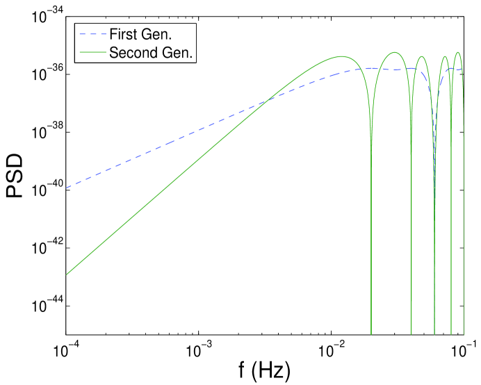
Figure 2: Plots of the first and second generation noise power-spectral densities (in units of Hz^-1).

III The Gravitational-wave Signal

Consider a GW source located at a distance $R$ relative to the solar system barycenter (SSB). Let $(\theta,\phi)$ denote the sky position of the source in the ecliptic coordinate system centered at the SSB. Then the sky-position vector is given by $\hat{\bf w}=(\sin\theta\cos\phi,\sin\theta\sin\phi,\cos\theta)$. In the transverse-traceless gauge MTW , the space-space part of the metric perturbation due to a gravitational wave emitted by this source and observed at the spacetime location (t, ${\bf r}$) can be expressed as

$$h_{mn}(t,{\bf r})=h_{+}(t-\hat{\bf w}\cdot{\bf r})(\theta_{m}\theta_{n}-\phi_{m}\phi_{n})+h_{\times}(t-\hat{\bf w}\cdot{\bf r})(\theta_{m}\phi_{n}+\theta_{n}\phi_{m})\ \ ,$$ (17)

where $m$ and $n$ are spatial indices, $\theta_{m}$ and $\phi_{n}$ are components of unit-normal vectors $\hat{\mbox{\boldmath$\theta$}}$ and $\hat{\mbox{\boldmath$\phi$}}$, respectively, that define a transverse plane with respect to the wave-propagation vector, $-\hat{\bf w}$, and $h_{+}$ and $h_{\times}$ are the two polarization components of the impinging wave. Therefore, the strain in LISA’s $i$th arm is characterized by the contraction of the arm’s “detector” tensor, $n_{i}^{m}n_{i}^{n}$, with the perturbation matrix $h_{mn}(t,{\bf r})$:

$$h_{i}(t)=h_{+}(t)\xi_{i+}(\theta,\phi)+h_{\times}(t)\xi_{i\times}(\theta,\phi)\ \ ,$$ (18)

where

$$\xi_{i+}(t)=(\hat{\mbox{\boldmath$\theta$}}\cdot\hat{\bf n}_{i}(t))^{2}-(\hat{\mbox{\boldmath$\phi$}}\cdot\hat{\bf n}_{i}(t))^{2}\hskip 10.0pt\quad{\rm and}\quad\xi_{i\times}(t)=2(\hat{\mbox{\boldmath$\theta$}}\cdot\hat{\bf n}_{i}(t))(\hat{\mbox{\boldmath$\phi$}}\cdot\hat{\bf n}_{i}(t))\ \ ,$$ (19)

define that arm’s beam pattern.

In this paper, we consider how well one would be able to estimate the parameters of a nearly monochromatic source, such as a low-mass compact binary, in the LISA data. Let the masses of the two stellar members of these sources be $m_{1}$ and $m_{2}$. Then, in the quadrupole approximation, the amplitude of its signal at the SSB can be expressed as Rogan:2004wq

$$H(\omega)=1.188\times 10^{-21}\left[{\mathcal{M}\over M_{\odot}}\right]^{5/3}\left[{R\over 1{\rm kpc}}\right]^{-1}\left[{\omega\over 2\pi\hskip 2.0pt{\rm mHz}}\right]^{2/3}.$$ (20)

where $\mathcal{M}=m_{1}^{3/5}m_{2}^{3/5}/(m_{1}+m_{2})^{1/5}$ is its chirp mass, $R$ is its luminosity distance, and $\omega\equiv 2\pi\nu$ is its angular frequency.

For a sufficiently high-mass binary, the inspiral of its members will cause the source frequency to increase perceptibly in the LISA band. On the other hand, for small chirp mass and emission frequency, as studied here, the rate of frequency evolution is approximately Rogan:2004wq

$$\dot{\omega}={48\over 5}\left({G\mathcal{M}\over 2}\right)^{5/3}\omega^{11/3},$$ (21)

where $G$ is the universal gravitational constant.

Both the amplitude and the phase of a GW signal will undergo modulation due to LISA’s changing orientation and motion relative to the source. The amplitude modulation is determined by the sky position angles and the source orientation. The latter can be specified in terms of the polarization angle, $\psi$, and the inclination, $\iota$, of the binary’s orbit relative to the line of sight. As was shown in Ref. Rogan:2004wq , this modulation in the $A$th pseudo-detector, arising from LISA’s $i$th arm, is captured by the complex extended beam pattern functions,

$$E^{A}_{i}:=T^{~{}\rho}_{2}\hskip 3.0ptD^{~{}A}_{\rho\hskip 1.0pti}\ \ ,$$ (22)

where the sum over the values of $\rho=\pm 2$ is implicit. The advantage of the above decomposition of the extended beam patterns is that all the source-orientation dependence is limited to the Gel’Fand functions GMS ; Bose:1999pj ; Pai:2000zt ,

$$T_{2}^{~{}\pm 2}\left(\psi,\iota,0\right)=\frac{1}{4}\left(1\pm\cos\iota\right)^{2}\exp\left(\mp{\rm i}2\psi\right)\,.$$ (23)

The influence of the source location and the arm orientation on the amplitude modulation is factored in

$$D_{\pm 2\hskip 1.0pti}^{A}={\omega L_{i}\over 2}|M_{i}^{A}|(\xi_{i+}\mp i\xi_{i\times})\ \ ,$$ (24)

where

$$M_{i}^{A}=q^{A}_{i-1}{\rm sinc}\left(\omega L_{i}{(1+\hat{\bf w}\cdot\hat{\bf n}_{i})\over 2}\right)-p^{A}_{i+1}{\rm sinc}\left(\omega L_{i}{(1-\hat{\bf w}\cdot\hat{\bf n}_{i})\over 2}\right)\,.$$ (25)

As was shown in Ref. Rogan:2004wq the strain in the $A$th pseudo-detector can be expressed as:

$$h^{A}(t)=H(\omega)\sum_{i=1}^{3}\Re\left[e^{-{\rm i}\delta}E_{i}^{A*}(t)S_{i}^{A}(t)\right]\ \ ,$$ (26)

where $\delta$ is the initial phase and

$$S_{i}^{A}\equiv e^{{\rm i}\omega(t-L_{i}\tau_{i})+{\rm i}({1\over 2}\dot{\omega}t^{2}+\sigma_{i}^{A})+{\rm i}\phi_{D}(t)}$$ (27)

describes the phase evolution of the signal. Above, $\sigma_{i}^{A}=\arg(M^{A}_{i})$ denotes the modulation in the phase arising from LISA’s changing beam patterns, and

$$\tau_{i}\equiv{1\over 2}\left(1-{\hat{\bf w}\cdot\hat{\bf r}_{i}\over\sqrt{3}}\right)\ \ ,$$ (28)

where $L_{i}\hat{\bf w}\cdot\hat{\bf r}_{i}/\sqrt{3}$ is the delay in the arrival of the signal at the $i$th craft relative to LISA’s centroid. Finally,

$$\phi_{D}(t)=\omega d_{\odot}\sin\theta\cos\left(\frac{2\pi t}{P}-\phi\right)$$ (29)

gives rise to the Doppler-phase modulation owing to LISA’s motion relative to the source. Here, $d_{\odot}$ (= 1 AU) is the average distance to the sun from LISA’s centroid and $P$ (=1 year) is the time taken for LISA to complete one full orbit around the sun.

The strain expression given in Eq. (26) will be used below to ascertain how well we can estimate a slightly chirping ($\dot{\omega}\neq 0$) binary’s parameters with LISA. The above discussion shows that such as signal will be characterized by eight parameters, $\mbox{\boldmath$\vartheta$}=\{T^{2}\dot{\nu},H,\delta,\psi,\cos\iota,\phi,\cos\theta,T\nu\}$, such that, $\vartheta^{0}=T^{2}\dot{\nu}$, $\vartheta^{1}=H$, …, and $\vartheta^{7}=T{\nu}$. Note that all parameters are dimensionless.

IV Estimating signal parameters

In estimating the parameters of a signal, an observer has to confront the inherently noisy nature of the detector or receiver, which introduces a degree of randomness in the parameter measurements. Thus, an ensemble of multiple copies of the detector will return a distribution of parameter values that is affected by the characteristics of the detector noise. The spread in the distribution indicates the noise-limited accuracy of the detector.

Before we define our estimator and determine its accuracy, note that even in the absence of instrumental noise, a typical detector has physical limits on its measurement accuracy. In this context, it is important to note that there are two important time-scales that affect LISA’s observations: The first arises from LISA’s orbital baseline, the mean light-travel time for which is close to 1000s. Thus, the frequency of a wave with wavelength equal to this distance is about 1mHz. The other scale arises from LISA’s 5 million-km arm-length, which corresponds to a light-travel time of 16.67s. Thus, waves with frequencies that are odd-integral multiples of 0.03Hz will drive the two craft at the ends of an arm out of phase by 180 degrees. This makes LISA’s sensitivity oscillatory at the higher end of its band (see Eqs. (II) and Fig. 2.)

To ascertain how large the noise-limited errors will be in the parameter values, we take the parameter values themselves to be the maximum likelihood estimates (MLEs). Owing to noise, the MLEs, $\hat{\mbox{\boldmath$\vartheta$}}$, can deviate from the true values of the signal parameters and can influence the determination of other parameters. The magnitude of these deviations and influences can be quantified by the elements of the variance-covariance matrix, $\gamma^{mn}=\{\hat{\vartheta}^{m},\hat{\vartheta}^{n}\}$ Hels .

A relation between the $\gamma^{mn}$ and the signal is available through the Cramer-Rao inequality, which dictates that

$$\parallel{\mbox{\boldmath$\gamma$}}\parallel~{}\geq~{}\parallel{\mbox{\boldmath$\Gamma$}}\parallel^{-1}\ \ ,$$ (30)

where $\Gamma$ is the Fisher information matrix:

$$\Gamma_{mn} = \sum_{A=1}^{2}\bigg{\langle}\partial_{m}h^{A}(\mbox{\boldmath$\vartheta$}),\partial_{n}h^{A}(\mbox{\boldmath$\vartheta$})\bigg{\rangle}_{(A)}$$ (31)

$$\equiv \sum_{A=1}^{2}{2\over P^{A}(f)}\int_{0}^{T}\left[\partial_{m}h^{A}(t;\mbox{\boldmath$\vartheta$})\right]\left[\partial_{n}h^{A}(t;\mbox{\boldmath$\vartheta$})\right]dt\,.$$

In this paper, we determine the values of $\Gamma_{mn}$ for signals from low-mass compact binaries in LISA data. Therefore, $\Gamma_{mm}^{-1/2}$ gives the lower bound on $\Delta\vartheta^{m}$ (which is the expected random error in the MLE of $\vartheta^{m}$). The two are equal in the limit of large SNR.

Since the amplitude and the initial phase are extrinsic parameters, one can analytically maximize the likelihood ratio with respect to them Rogan:2004wq . Here, we assume that this has been done. In such a case, the Fisher information matrix is six-dimensional. The errors in the phase and the amplitude can be derived in terms of the errors in the remaining six parameters as demonstrated, e.g., in Ref. Jaranowski:2005hz . This is the method we use to compute the error in $H$. One can similarly infer the error in $\delta$.

The errors in the sky-position angles will be presented in terms of the error in the measurement of the sky-position solid angle, defined as:

$$\Delta\Omega_{S}=2\pi\left(\Delta\vartheta^{5}\Delta\vartheta^{6}-\langle\Delta\vartheta^{5}\Delta\vartheta^{6}\rangle\right)\,.$$ (32)

We define the error in the measurement of the source-orientation solid angle similarly:

$$\Delta\Omega_{L}=2\pi\left(\Delta\vartheta^{3}\Delta\vartheta^{4}-\langle\Delta\vartheta^{3}\Delta\vartheta^{4}\rangle\right)\ \ ,$$ (33)

where the subscript $L$ denotes the orbital angular momentum of the binary.

IV.1 Scaling of parameter errors with SNR

Although our expressions above can be used to compute the error estimates for any parameter values, we illustrate our results for specific values of some of these parameters: Unless specified otherwise, we use an integration time of one year, an emission frequency of $\nu=3$ mHz, and source orientation angles $\psi={\pi/3}$ and $\iota={\pi/4}$. The emission frequency is chosen to be large enough so that the Doppler-phase modulations have a significant effect. The source orientation is chosen somewhat arbitrarily, except that we ensure that the signal is not linearly polarized.

All the parameter estimates studied below are obtained by normalizing the estimates given in Eq. (31) by the network sensitivity, $\left[\sum_{A=1}^{2}\langle h^{A},~{}h^{A}\rangle_{(A)}\right]^{-1}$. Thus, the parameter-estimate values shown in the plots here are for a signal with an SNR of 1. To get an estimate for an arbitrary SNR, one simply multiplies the value shown in the plots by the SNR scale given in Table 1.

Table 1: The table lists how the errors in different parameters scale with the SNR. Since all our error plots are given for an SNR of unity, to assess the error for any other SNR one simply needs to multiply the plot value with the scale read from this table.

	$\quad\Delta\Omega_{S}\quad$	$\quad\Delta\Omega_{L}\quad$	$\quad\Delta H/H\quad$	$\quad T\Delta\nu\quad$	$\quad T^{2}\Delta\dot{\nu}\quad$
SNR scale	$\quad{\rm SNR}^{-2}\quad$	$\quad{\rm SNR}^{-2}\quad$	$\quad{\rm SNR}^{-1}\quad$	$\quad{\rm SNR}^{-1}\quad$	$\quad{\rm SNR}^{-1}\quad$

An alternative way of understanding the parameter estimate normalization is through the Fisher information matrix. The idea here is to first divide the Fisher information matrix by the network template norm, $\sum_{A=1}^{2}\langle h^{A},~{}h^{A}\rangle_{(A)}$, as follows:

$$\widehat{\Gamma}_{mn}=\frac{\Gamma_{mn}}{{\sum_{A=1}^{2}\langle h^{A},~{}h^{A}\rangle_{(A)}}}\,.$$ (34)

One then obtains the normalized error estimates from the covariance matrix derived by inverting $\widehat{\Gamma}_{mn}$.

V Doppler-phase modulation

When a template does not track the Doppler-phase modulation of a signal, over time it gets increasingly phase-incoherent relative to the latter. We quantify the degree of coherence between the two by the fitting factor:

$$m(\mbox{\boldmath$\vartheta$},\mbox{\boldmath$\vartheta$}^{\prime})={\sum_{A=1}^{2}\langle h^{A}(\mbox{\boldmath$\vartheta$}),h^{A}(\mbox{\boldmath$\vartheta$}^{\prime})\rangle_{(A)}\over\sqrt{\sum_{B=1}^{2}\langle h^{B}(\mbox{\boldmath$\vartheta$}),h^{B}(\mbox{\boldmath$\vartheta$})\rangle_{(B)}\>\sum_{C=1}^{2}\langle h^{C}(\mbox{\boldmath$\vartheta$}^{\prime}),h^{C}(\mbox{\boldmath$\vartheta$}^{\prime})\rangle_{(C)}}}\ \ ,$$ (35)

where the value of the “template parameter” $\mbox{\boldmath$\vartheta$}^{\prime}$ is, in general, different from that of the “signal parameter” $\vartheta$. The plot of the above function, with $h^{A}(\mbox{\boldmath$\vartheta$}^{\prime})$ as the template without Doppler shifting and $h^{A}(\mbox{\boldmath$\vartheta$})$ as the signal with that shifting accounted for, is given in Fig. 3. As can be inferred from that figure, when the Doppler-phase modulation is not accounted for in the search templates, the SNR suffers an appreciable drop across the entire LISA band. It also exhibits large oscillations with a period that depends on LISA’s orbital speed and that decreases linearly with increasing source frequency, as is characteristic of Doppler frequency shifting. It is important to note the locations of the nodes in the plot: The first minimum is at approximately $f=$1/2L, which occurs when the phases of a gravitational wave impinging along an arm are different by 180^∘ at the two craft at the two ends of that arm.

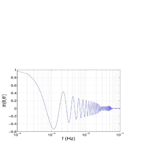
Figure 3: This is a plot of the fitting factor between two similar templates, one with the Doppler-phase modulation included and the other without it.

In conclusion, since the effect of discounting Doppler-phase modulation is so marked on the SNR at any LISA frequency of interest, one must account for its effect on parameter estimation throughout the LISA band.

VI Effect of source frequency evolution

For binary compact object that are spiraling in fast enough, LISA will be able to measure their chirp mass and luminosity distance. Expression (20) shows that the amplitude, $H(\omega)$, of a signal from such an object depends jointly on $r$ and ${\cal M}_{c}$. However, neither of these parameters affects any other part of a monochromatic (or $\dot{\nu}$) signal, as given in Eq. (26). Thus, one can not separately estimate either of them purely from the amplitude. Nevertheless, if a signal has an appreciable amount of inspiral or frequency evolution, defined in Eq. (21), then the measurement of $\dot{\nu}$, along with $H(\omega)$, determines both the chirp mass and the source distance.

In order to ascertain the individual masses of the binary, additional information is necessary. Traditional astronomical methods using optical or radio measurements can be used to help identify the total mass of the binary system. However for many unknown sources or optically invisible sources this is not an option. In some cases where the binary orbit is noticeably eccentric, the accurate tracking of the emission frequency can provide information on the total mass of the system. This datum, together with the chirp mass, can be used to infer the individual masses of the system Seto:2001pg .

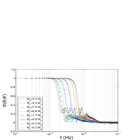
Figure 4: Fitting factors of low-mass compact binaries with a range of chirp masses are plotted as functions of frequency. Here the fitting factor is between two template families, one with a physical set of eight parameter values and another with the chirp ($\vartheta^{0}$) set to zero, artificially, for all source frequencies. For the above plots, the sources are located on the ecliptic, with $\theta=\pi/2$, $\phi=\pi/2$, and their orientation is $\iota=\pi/4$, $\psi=\pi/3$. As a reference, an equal-mass binary, with $m_{1}=m_{2}\equiv 0.35~{}M_{\odot}$ has ${\cal M}_{c}=0.3~{}M_{\odot}$. Fitting factors for equal-mass binaries with $m=$1,2,3,…6$~{}M_{\odot}$ can also be read from here.

Before analyzing the quantitative effects of a chirping waveform on parameter estimation we briefly study the role that a non-negligible $\dot{\nu}$ plays in searching for a signal. Specifically, we use the fitting factor defined in Eq. (35) to determine the fractional loss in the SNR while searching for a chirping source with monochromatic (i.e., $\dot{\nu}=0$) templates. When subtracted from unity, the above function measures the fractional drop in the SNR owing to a parameter mismatch of $\Delta\mbox{\boldmath$\vartheta$}\equiv\mbox{\boldmath$\vartheta$}-\mbox{\boldmath$\vartheta$}^{\prime}$. In Fig. 4, we plot $m(\mbox{\boldmath$\vartheta$},\mbox{\boldmath$\vartheta$}^{\prime})$ with $\Delta\vartheta^{m}=0$, for all $m\neq 0$; the “template parameter”, $\vartheta^{\prime\>0}$, is set to zero, while the “signal parameter”, $\vartheta^{0}$, is determined by Eq. (21) for any given emission frequency and chirp mass. For any given chirp mass, note how rapidly the SNR drops as a function of frequency. Also, since at any given frequency the chirping causes a smaller mismatch between the two template families for a smaller chirp mass, the SNR drop occurs at a higher frequency for a smaller chirp mass. Just like Fig. 3, this fitting factor too has oscillatory features. However, owing to the polynomial frequency behavior of $\dot{\nu}$, the oscillations here do not exhibit the linear decrease in the node-spacing found in Fig. 3.

We now turn our attention to the role of $\dot{\nu}$ in the estimation of the signal parameters. As shown in Sec. IV, the expansion of the template parameter space in order to include another parameter affects the parameter estimation through the Fisher information matrix, which is a different construct than the fitting factor. Once a detection has been made, the error values presented here provide the standard deviation that should be expected for an ensemble of signal measurements made by LISA. However, one still needs to establish for what ranges of $\omega$ and ${\cal M}_{c}$ it is possible to measure a non-vanishing chirp in a signal. Outside these ranges, including $\dot{\omega}$ in ones template-parameter space can result in worse estimates for other parameters. A smaller parameter volume for estimating parameters is also desirable because it leads to a lesser computational burden: This is more so since the problem of detection in the presence of LISA’s source confusion noise is intricately linked with the problem of parameter estimation.

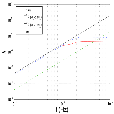
Figure 5: These plots illustrate the values (in number of cycles) of the chirp parameter for two values of the chirp mass (${\cal M}_{c}=0.3M_{\odot}$ and $5.3M_{\odot}$), along with the errors in determining the chirp and frequency for an SNR of 10. All plots are for an observation period of $T=1$ year. Note how for the larger chirp mass the error in determining the chirp remains comparable to the value of the chirp itself up to about 1.5mHz, before improving at higher frequencies.

Figure 5 shows that for binaries with ${\cal M}_{c}\simeq 5.3~{}M_{\odot}$, the error in the estimation of its chirp is at least as large as the value of the chirp itself (for an SNR of 10) for $\nu\lower 2.15277pt\hbox{$\;\buildrel<\over{\sim}\;$}2.5$ mHz. As shown in Fig. 6, this is very close to the frequency where the inclusion of the chirp starts hurting the estimation of the frequency. On its own merit, this would argue for the dropping of the $\dot{\nu}$ parameter from the search templates (i.e., setting $\vartheta^{0}=0$) for ${\cal M}_{c}\lower 2.15277pt\hbox{$\;\buildrel>\over{\sim}\;$}5.3~{}M_{\odot}$ and $\nu\lower 2.15277pt\hbox{$\;\buildrel<\over{\sim}\;$}2.5$ mHz. However, the fitting factor plot shows that doing so can vastly reduce the probability for detecting such signals with $\nu\lower 2.15277pt\hbox{$\;\buildrel>\over{\sim}\;$}1$ mHz. We have thus, identified a region in the parameter space where entertaining the prospects of a detection requires taking a beating in estimating the source parameters. This adds an additional layer of challenge in the quest for cleaning what is deemed as the resolvable part of the confusion noise spectrum.

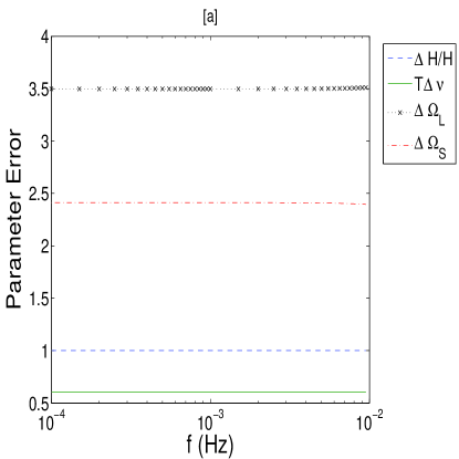
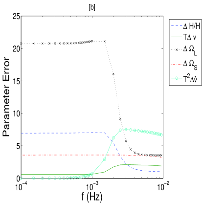
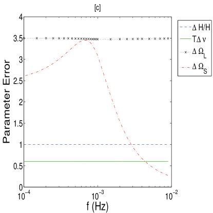
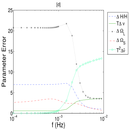
Figure 6: These figures show how the errors in the different signal parameters behave as a function of the source frequency for the following four cases (a) with no Doppler-phase modulation and no chirp, (b) with chirp only, but no Doppler-phase modulation, (c) with Doppler-phase modulation, but no chirp, and (d) with both Doppler-phase modulation and chirp included. The sky-position assumed is: $\theta=\pi/2$, $\phi=\pi/2$; also, $\iota=\pi/4,~{}\psi=\pi/3$.

VII Frequency Dependence of parameter errors

Imagine a one-parameter family of sources, which have everything else identical, except for the emission frequency, $\nu$. The parameter-estimation errors for such a family are not invariant across LISA’s bandwidth. This is because both the Doppler-frequency shifting and the frequency evolution increase with $\nu$. Additionally, the sensitivity of LISA itself varies across the band, as shown in Fig. 7. For nearly monochromatic signals, the latter effect gets essentially factored away when considering SNR-normalized estimates. Figure 6 shows the frequency dependence of the parameter errors, normalized for an SNR of unity, for four different cases: Case (a) depicts these errors when a signal has no Doppler-phase modulation, and no frequency evolution (where the latter is unphysical). Case (b) presents the same when there is frequency evolution natural to the binary, but no Doppler-phase modulation (such as if LISA were at the SSB). Case (c) includes the effect of Doppler phase modulation but has the frequency evolution (artificially) turned off. Finally, plot (d) has effects from both the Doppler phase modulation and the frequency evolution.

Figure 7: These are plots for the sensitivity of LISA as a function of the frequency (in Hz) for the first and second generation TDIs, respectively.

It is interesting to note that in Fig. 6a the error in the estimate of each of the parameters is essentially independent of the emission frequency. The primary contribution to the frequency dependence of the Fisher information matrix in Eq. (31) arises from LISA’s own sensitivity reflected in its noise PSD. The elements of this matrix depend on $P^{A}(f)$, which is the same for both $A=1,2$. However, when the parameter errors are obtained by scaling this matrix by the template norm, as described in Eq. (34), the factor of $P^{A}(f)$ for near-monochromatic signals gets canceled away, thus rendering the plots in Fig. 6 mostly flat.

We next consider the effect of Doppler-phase modulation on the parameter estimation accuracy. Comparing Figs. 6a and 6c shows that the errors in all parameters are mostly unaffected except for the error in sky-position. That error actually worsens with frequency in the 0.1-1 mHz band, before rapidly improving at higher frequencies. This is because at wavelengths longer than 1 AU, the Doppler-phase modulation acts like noise on the sky-position dependent $\sigma^{A}_{i}$ term in the phase of the signal in Eq. (27), thus, affecting sky-position estimation. On the other hand, at high frequencies, it does a better job at resolving a binary’s direction than do the beam-pattern-function induced modulations of the amplitude and the phase.

The effect of the chirp can be understood by comparing Figs. 6c and 6d (or, alternatively, Figs. 6a and 6b): It worsens the estimation of the amplitude and source orientation at low frequencies, i.e., for $\nu\lower 2.15277pt\hbox{$\;\buildrel<\over{\sim}\;$}1.5$ mHz. It also reduces the accuracy of its own estimate and that of the source frequency at high frequencies, i.e., for $\nu\lower 2.15277pt\hbox{$\;\buildrel>\over{\sim}\;$}1.5$ mHz. Here, one may wonder why at frequencies below 1.5 mHz, the chirp’s inclusion ruins the determination of the source orientation, but not the frequency. The answer is that during the course of a year one integrates through a very large number of cycles of a signal, which averages out the noise in the estimation of the frequency arising from the chirp. The same would be true about the orientation if one were to integrate for a large number of LISA orbits (or years). Interestingly, at frequencies higher than 2 mHz, while the chirp leaves the estimation of the source orientation unaffected, it hurts the estimation of the source frequency. This is because starting at around a milli-Hertz, the chirp acts as a source of noise in the determination of the frequency.

In summary, the general behavior of the SNR normalized parameter-estimation errors as functions of $\nu$ can be understood as follows. Primarily, there are two competing parts of the signal that provide information about the source: The amplitude modulation and the phase modulation. The amplitude is modulated differently throughout the course of a year depending on the source location and orientation. The amplitude modulations provide information about these two source parameters in a manner that the SNR-normalized error in them remains invariant across LISA’s band (as can be inferred from Fig. 6 a). Whereas tracking the phase provides information about the source location, source frequency, frequency evolution and, hence, the chirp mass. The main difference between the two modulations is that the phase modulation is highly dependent on the emission frequency of the source, whereas amplitude modulation is not. Since the amplitude modulation is less sensitive to the emission frequency, its contribution to any parameter estimate is relatively unchanged over LISA’s band. Contrastingly, phase modulation provides less information at low emission frequencies. This is due to the relatively fewer cycles one obtains in a given observation time for low frequencies compared to higher ones. For the frequency range that LISA is projected to observe, this translates into roughly a factor of $10^{3}$ less cycles that would be obtained for the smallest observable frequencies with respect to the largest ones. However, as the frequency increases the contribution from the phase modulation eventually surpasses that due to the amplitude modulations.

VII.1 Excluding frequency evolution from the templates

The preceding discussion shows that at any given LISA frequency searching for the frequency evolution of a binary affects the determination of one or the other parameter, except the sky position. For a source with an initial frequency, $\nu\lower 2.15277pt\hbox{$\;\buildrel>\over{\sim}\;$}1.5$ mHz, its inspiral hurts the error in the estimation of $\nu$ by a factor of over 3.5 relative to that of sources with $\nu\lower 2.15277pt\hbox{$\;\buildrel<\over{\sim}\;$}1$ mHz. We have verified that increasing the integration time to 2 years reduces this relative error factor to about 2, confirming what is shown in Ref. Takahashi:02 . This reduction may be insufficient for the resolution of the galactic binary confusion noise. This makes a case for a mission lifetime that is longer than 2 years. Otherwise, the only other option available for maintaining the parameter accuracies is to exclude the chirp parameter from the search templates, since doing so improves the SNR-normalized parameter estimates. This, however, has different consequences for the parameter accuracies of binaries with different chirp masses.

The fitting-factor plots in Fig. 4 show that for the lowest astrophysically interesting chirp mass, ${\cal M}_{c}\simeq 0.3M_{\odot}$, such an exclusion has little effect on the SNR until about 4 mHz, which happens to be just below the high-frequency-end of the confusion noise arising from extreme mass-ratio inspiral (EMRI) sources. The effect on the estimates of the other parameters is a systematic bias by an amount that depends linearly on $T^{2}\dot{\nu}$ BoseRoganPrep1 , which is about 0.1 (cycles) for $T=1$year and at $\nu=4$ mHz. While this introduces a negligible bias in the estimates of all parameters, it has the advantage of reducing the level of the random estimation errors to the same level as that shown in Fig. 6a. At frequencies as high as even 6 mHz, the SNR drop due to such an exclusion would be more than 30%, thus, jeopardizing both the prospects of detection and the adequate parameter resolution required for cleaning the WD-WD confusion noise.

On the other hand, note that for a binary with ${\cal M}_{c}\geq 5.3M_{\odot}$, such an exclusion causes the same fractional drop in the SNR at frequencies as low as 1.5 mHz, which is where the parameter estimates start getting affected (see Fig. 6b or 6d). Thus, for binaries with ${\cal M}_{c}\geq 5.3M_{\odot}$, turning off the chirp parameter in the search templates is unlikely to improve the parameter estimation for $\nu\geq 1.5$ mHz. Among the sources most affected from this “chirp search” problem are galactic low-mass binaries containing a black hole.

VIII Sky-position dependence of parameter errors

In this section, we study the behavior of the parameter errors as functions of the direction to a binary. We illustrate the sky-position dependence of the SNR-normalized parameter errors for the same source polarization state and frequency as the one chosen in Sec. VII for the frequency plots in Fig. 6. The source frequency choice, viz., $\nu=3$ mHz is interesting for multiple reasons: As observed above, it is close to the high-frequency-end of the unresolvable WD-WD confusion noise. Figure 6d shows that it is also in the region of transition in the behavior of the parameter errors as functions of frequency. All the same, it is not too small for the Doppler-phase modulation to have a negligible effect on the parameter accuracies.

When studying these errors as functions of frequency in Fig. 6, we had fixed the sky position of the source. For this reason, while computing the SNR-normalized errors, we did not have to worry about the possibility that the SNR may vary with the sky position. We begin by addressing that possibility below. The dependence of the SNR on the polarization state can be studied similarly.

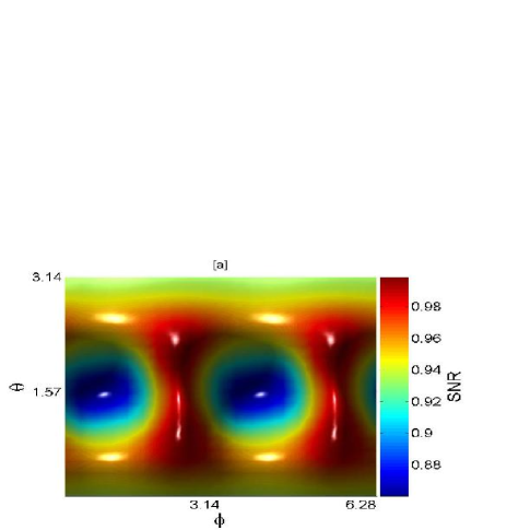
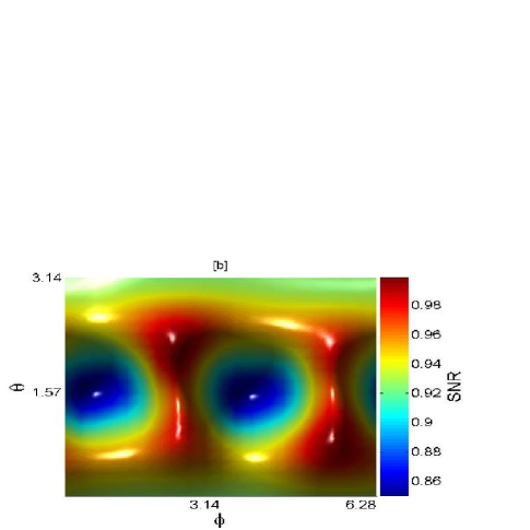
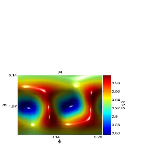
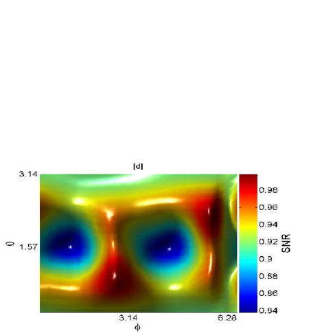
Figure 8: These are plots of the template-norm-squared for the same four cases of LISA motion and source frequency evolution considered in Fig. 6. The plot for each case is normalized to have a maximum value of unity. Both $\theta$ and $\phi$ are given in radians, with the origin, $(0,0)$, in the bottom left corner of each plot. Note that this is the first of a series of colored sky-plots; gresyscale prints of these plots can give a misleading impression of the color values.

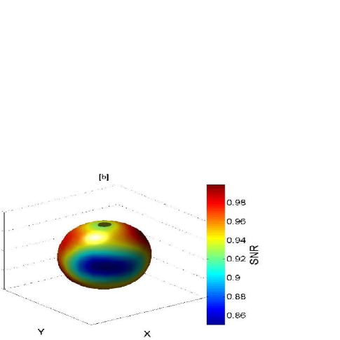
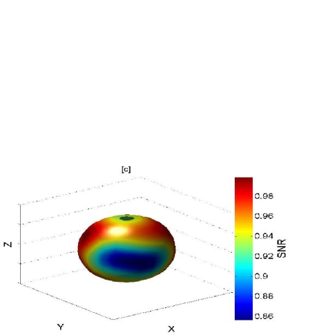
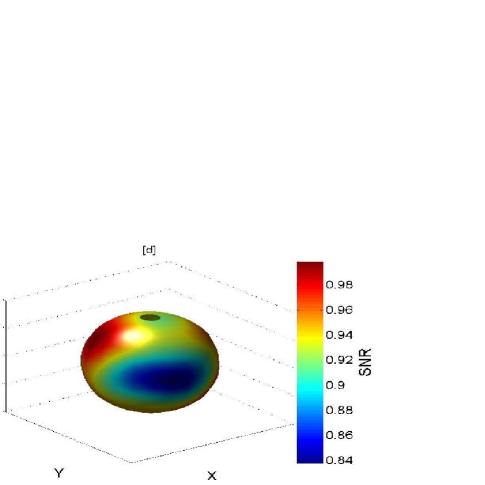
Figure 9: Spherical renditions of the template-norm-squared plots shown in Fig. 8.

VIII.1 Sky-position dependence of the SNR

The SNR normalization performed on the Fisher information matrix in Eq. 34 is useful in that the parameter errors computed from such a matrix can be easily scaled for a signal of any SNR using the scaling factors given in Table 1. In this context, it is important to note that the SNR of a standard candle is not uniform across the sky owing to the non-uniform sensitivity of LISA to different sky positions. We plot this quantity for four different cases in Figs. 8 and 9, where the latter set is the 3D rendition of the former set. These plots, called “sky plots”, are normalized so that the maximum value attained in each case is unity. These four cases are identical to those considered for studying the frequency dependence of parameter errors in Figs. 6. As in that study, here too Fig. 8a (or, equivalently, Fig. 9a) is for an artificial signal, with $\dot{\nu}$ set to zero), when compared with Fig. 8b, it allows one to graphically assess how useful or detrimental the presence of frequency evolution is in detecting a signal. Similarly for Fig. 8c, when compared with Fig. 8d. Note that as per the definitions of cases (a) and (b), Figs. 8a and 8b have the Doppler-phase modulation turned off.

VIII.2 Explaining the sky-position dependence

Given that LISA’s orbital motion is confined to a nearly circular orbit on the ecliptic, one may expect the SNR plots to be axisymmetric. This is indeed the case for the network comprising the two Michelson variables, as can be seen in Fig. 10, where we limit our focus to their geometric sensitivity and momentarily ignore the fact that they will be severely limited by the laser frequency-fluctuation noise. Figures 10a and 10b reveal that although the SNR for neither of the Michelson variables is axisymmetric, their quadrature combination is so. For comparison, we present the analogous plots for the $\bar{A}$ and $\bar{E}$ TDI variables in Figs. 11. We normalize all these plots relative to the maximum value attained among the template norms of the individual Michelson and $\bar{A}$-$\bar{E}$ variables.

Interestingly, however, the SNRs for the $\bar{A}$ and $\bar{E}$ TDI variables, plotted in Fig. 11, are more dumbbell-shaped than axisymmetric, where the pattern depends on the initial orientation of LISA. Also, since there is a slight difference between the overall sensitivities of the two variables, their quadrature combination is more of an inflated version of the $\bar{A}$ variable. As one would expect, it also resembles well the SNR of Fig. 9a.

Figure 12 illustrates the sensitivity of a single arm to all sky positions. What is evident from this figure is its striking similarity to the $\bar{A}$ TDI data combination. The features of this plot are well understood geometrically. For a single arm, spinning and orbiting the SSB, there exists a periodicity of $\pi$ radians under axial rotations. However, this figure shows that there are two distinct and orthogonal directions, and their antipodes, that stand out. These locations correspond to the global maxima and minima in the sensitivity of this arm to impinging gravitational waves. These very same extrema are present in the SNR plots as well. To understand the origin of these global extrema, the orbital motion of LISA’s centroid is not as important as the spin of LISA’s individual arms. Therefore, consider how a single arm spins during the course of a year. Let it begin in an orientation that is parallel to the ecliptic plane. In this orientation, a low-frequency source that is in a direction perpendicular to the arm will create the maximum strain in that arm. Conversely, when such a source is in a direction along the arm, the strain caused in that arm is zero. Let us call these directions 1 and 2, respectively. With the exception of their antipodes, there is no other orbital position that will attain such extrema in the sensitivity for that particular arm during its orbit. As the arm rotates out of the ecliptic plane, the sensitivity to direction 1 will begin to degrade. However, because direction 1 will never be parallel to the same arm, it will never attain the same minima that direction 2 attained initially and, vice versa. Therefore, the orbital position where these global extrema are obtained is forever imprinted upon the integrated results regardless of the duration of observation.

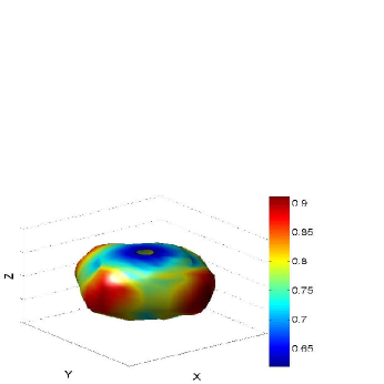
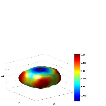
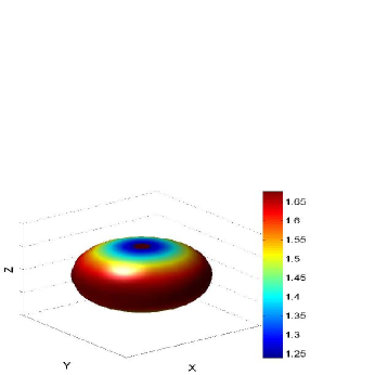
Figure 10: The template-norm-squared for the Michelson variables as functions of sky position: for Michelson variable I as a function of sky position (left), II. for Michelson variable II as a function of sky position (center), III. for the network comprising both Michelson variables (right). All plots are presented for the following source parameters: $\{\iota=\pi/4,\psi=\pi/3,\nu=3~{}{\rm mHz}\}$

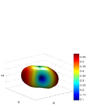
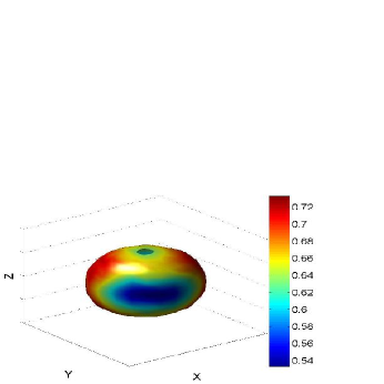
Figure 11: The template-norm-squared for the $\bar{A}$ and $\bar{E}$ TDI variables as functions of sky position: I. for the $\bar{A}$ TDI data combination (left), II. for the $\bar{E}$ TDI data combination as a function of sky position (center), and III. for the the network comprising both $\bar{A}$ and $\bar{E}$ TDI data combinations. All plots are presented for the following source parameters: $\{\iota=\pi/4,\psi=\pi/3,\nu=3~{}{\rm mHz}\}$.

VIII.3 Parameter errors

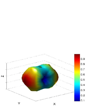
Figure 12: A single arm’s template-norm-squared. All plots are presented using the following parameters: $\{\iota=\pi/4,\psi=\pi/3,\nu=3~{}{\rm mHz}\}$.

We plot the parameter errors as functions of sky position in Figs. 13, 14, and 15 for the same source polarization state and frequency as described earlier in this section. Note that these parameter-error sky plots are presented for the $\bar{A}\bar{E}\bar{T}$ pseudo-detector network. Altering $\nu$, the polarization state, or the pseudo-detector network will, in general, change the details found in these plots. However, certain qualitative aspects, discussed below, will remain unaffected.

While all four cases (i.e., (a)-(d)) are plotted for sky-position and frequency errors in Figs. 13 and 14, respectively, only the full case (i.e., case (d)) is plotted for the remaining parameters in Fig. 15. This is because the plot for each case of these remaining parameters strongly resembles the frequency-error sky plot of the corresponding case in Fig. 14. Indeed, a quick examination of all the error plots reveals that they can be divided into two sets based on their apparent symmetry: (1) those for the sky-position and (2) those for the rest of the parameters. The first set displays a strong axisymmetry (i.e., symmetry with respect to translations along the $\phi$ axis) that is missing in the other set. The reason behind this divide is that the Fisher information matrix and, therefore, the parameter covariance matrix, is predominantly block diagonal, with two blocks. The first block comprises just the sky-position ($\theta$, $\phi$) variance-covariance and the second one comprises the variance-covariance of the rest of the parameters. The elements outside of these two blocks are not all zeros, but are much smaller than the elements within the blocks. Consequently, any error in a parameter in one set influences that in another parameter from the same set much more strongly than in the other set. This explains why the patterns in each case of the second set are so similar among all parameters within that set, as is manifest in Fig. 15. Also, the reason why the sky-position error plots are predominantly axisymmetric while the other ones are not is because while the latter are affected by the beam-pattern functions alone, the former are affected by them as well as their parameter derivatives. It is worth noting that the deviation from axisymmetry is still apparent in Figs. 13, however, this effect is significantly reduced with respect to the other parameters.

There is an alternative way of understanding the three “unphysical” cases (i.e., cases (a)-(c)) studied in Figs. 13 and 15. Starting with the last of these, case (c), note that it is identical to the physical case where the chirping is negligible. This is indeed the case when the chirp mass is as low as 0.3$M_{\odot}$. As seen in Fig. 4, for such a case, filtering the data with chirp-less templates causes negligible SNR loss. Thus, the case (c) plots in these figures indicate the expected random errors in such a search.

Case (b) resembles the physical case where the Doppler-phase modulation is negligible, which occurs when the source frequency is below a milli-Hertz (barring the slight ruining of the sky-position estimates). Since the chirp rate was fixed in this plot, to compensate for lowering the frequency to below 1 mHz one must increase the chirp mass, which affects the signal amplitude but not the SNR-normalized error shown here. Thus, case (b) is the expected error plot for all sources that have frequencies less than about 1 mHz but chirp masses commensurately larger than 5.3$M_{\odot}$ (such that ${\cal M}_{c}^{5/3}\omega^{11/3}=$ constant). Comparing the plots for cases (b) and (d) then shows that the SNR-normalized error tends to increase at low frequencies, more so at the poles than near the ecliptic.

Finally, case (a) represents the physical case where $\nu<1$ mHz and ${\cal M}_{c}$ is very small, such that both Doppler-phase modulation and source chirping are negligible. (Note that the sky-position error is almost constant in the LISA band below 1 mHz (cf. Fig. 6).) However as Fig. 3 illustrates, this will not occur in the LISA band.

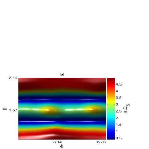
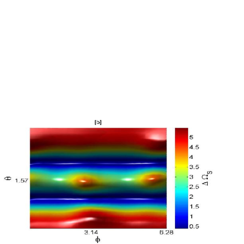
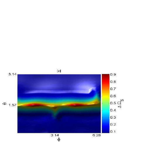
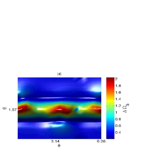
Figure 13: These are plots of the errors associated with determining the sky position measured in terms of a solid angle spread $\Delta\Omega_{S}$. The four plots are for the four cases described in Fig. 6. All plots are made for the following source parameters: $\{\iota=\pi/4,\psi=\pi/3,\nu=3~{}{\rm mHz}\}$.

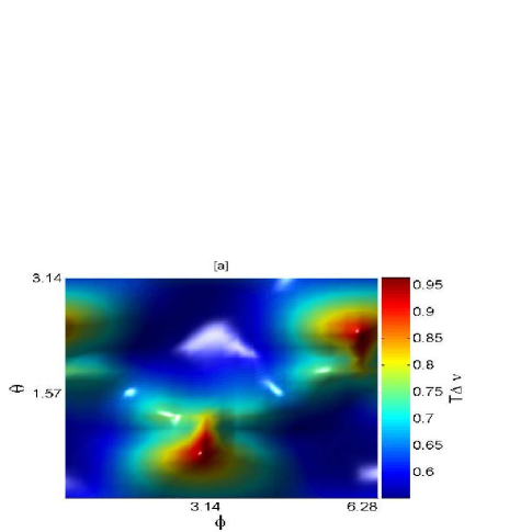
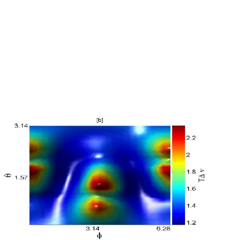
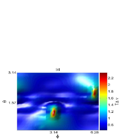
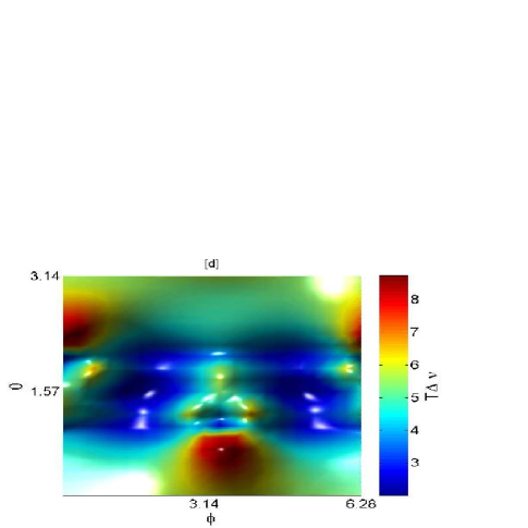
Figure 14: These are plots of the errors associated with determining the dimensionless emission frequency parameter $T\Delta\nu$. The four plots are for the four cases described in Fig. 6. All plots are made for the following source parameters: $\{\iota=\pi/4,\psi=\pi/3,\nu=3~{}{\rm mHz}\}$.

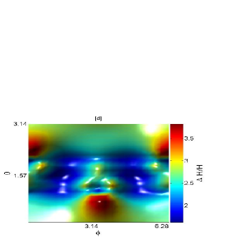
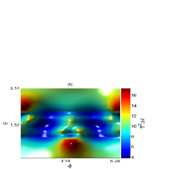
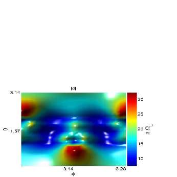
Figure 15: Plots of the errors associated with the remaining parameters: $\Delta H/H$, $T^{2}\Delta\dot{\nu}$, and $\Delta\Omega_{L}$. They all correspond to case (d) described in Fig. 6. Both Doppler-phase modulation and frequency evolution are included here. All plots are made for the following source parameters: $\{\iota=\pi/4,\psi=\pi/3,\nu=3~{}{\rm mHz}\}$.

IX Conclusion

In this paper we studied the effect of Doppler-phase modulation, frequency evolution, and time-delay interferometry on the accuracy of estimating signal parameters of low-mass circular binaries. All results presented here were obtained for maximum-likelihood estimates of binary signal parameters in a specific network of LISA’s TDI variables, namely, the $\bar{A}\bar{E}\bar{T}$ variables, and for a one-year integration time. We find that Doppler-phase modulation not only improves the sky-position estimation accuracy for $\nu\lower 2.15277pt\hbox{$\;\buildrel>\over{\sim}\;$}1$ mHz, but also degrades it in the range $0.1{\rm mHz}\lower 2.15277pt\hbox{$\;\buildrel<\over{\sim}\;$}\nu\lower 2.15277pt\hbox{$\;\buildrel<\over{\sim}\;$}1$ mHz. It also increases the error in the chirp parameter by a factor of 2 and the frequency by a factor of 1.5 at $\nu\simeq 10$ mHz. It leaves the accuracies of the remaining parameters, namely, the source orientation and the signal amplitude mostly unaffected.

The exclusion of the chirp (or frequency evolution) parameter affects the SNR loss by different amounts for binaries with different chirp masses. For instance, Fig. 4 shows that for ${\cal M}_{c}\lower 2.15277pt\hbox{$\;\buildrel<\over{\sim}\;$}5.3~{}M_{\odot}$, such an exclusion causes negligible effect on the SNR for $\nu\lower 2.15277pt\hbox{$\;\buildrel<\over{\sim}\;$}1$ mHz. Since in this low-frequency band the estimation accuracy of all signal parameters, except $\nu$ and $\dot{\nu}$, is affected by its inclusion, from a few percent for the sky-position error to a factor of 6 for the source orientation, it is advisable to drop the chirp parameter from the search templates for these sources. On the other hand, since the SNR loss from excluding the chirp parameter cannot be ignored when $\nu\lower 2.15277pt\hbox{$\;\buildrel>\over{\sim}\;$}3$ mHz, for all but the lowest chirp masses of interest, one has to accept the parameter-error consequences for these high frequency sources. Luckily, a majority of the parameters remain unaffected in this high-frequency band, except $\nu$ and $\dot{\nu}$. Thus, if one were to turn off or on the inclusion of the chirp parameter judiciously, so as to get the most accurate estimates possible for $\Omega_{L}$, $\Omega_{S}$, $H$, then for a given chirp mass, the error profiles in the frequency plots would be such that they are low (i.e., at the levels shown in Fig. 4a) at the low frequencies, but rise at the mid-frequencies, and fall off at the high frequencies as in Fig. 4d. The biggest casualty arising from searching for the chirp at high frequencies is $\dot{\nu}$: its error can suffer by as much as a factor of 5 at frequencies greater than 3 mHz (see Fig. 6d). A similar conclusion was arrived at earlier by Takahashi and Seto Takahashi:02 while working with the Michelson variables, although their exact numbers were somewhat different. Clearly, this will have an adverse effect on the resolvability of the confusion noise above 3 mHz.

Comparing the frequency plots we obtained here to those found in Ref. Takahashi:02 , one striking aspect is the reduced levels for the SNR-normalized errors we find for most parameters at all frequencies. Its origin lies in the two principal differences between our studies, namely, the choice of the data variables (TDI versus Michelson variables) and the approximations made in Ref. Takahashi:02 . For instance, the value of $\Delta H/H$ presented in Takahashi:02 is its average over LISA’s band, whereas we derive the values of $\Delta H/H$ for different frequencies. Also, we do not use the long-wavelength approximation, which has been shown to have significant effects at frequencies above 3mHz Vecchio:2004ec .

One of the many interesting astrophysical sources that LISA can target is a stellar-mass binary containing a black hole. It is unclear how many such objects are present in our galaxy. These objects will likely have chirp masses in excess of 2$M_{\odot}$. Figure 4 shows that for $\nu\lower 2.15277pt\hbox{$\;\buildrel>\over{\sim}\;$}2$ mHz, detecting them will require inclusion of the chirp parameter in the search templates. This, however, will result in large inaccuracies in all of its parameters in the range 2-3 mHz. That in turn will hamper our ability to discern their signals from those of the confusion noise, unless their SNRs are sufficiently large. A large SNR can result either from the proximity of a source or a large chirp mass or both. A large chirp mass, however, will not always serve this purpose because the 2-3 mHz range actually widens towards lower frequencies with increase in chirp mass. This is because the point at which $m(\mbox{\boldmath$\vartheta$},\mbox{\boldmath$\vartheta$}^{\prime})$ starts deviating from unity in Fig. 4 shifts to lower frequencies with increasing ${\cal M}_{c}$. This identifies a problem with LISA’s ability to detect stellar mass black hole binaries, about which very little is known in terms of their formation and demographics.

Note that the above conclusions will change, in general, as the integration time is increased. For example, a ten-year integration time will not only improve the accuracy with which the chirp parameter will be determinable, but also reduce the adverse effects that its inclusion in search templates has on the estimation accuracy of other parameters Takahashi:02 . Some changes may also appear in the SNR-normalized frequency and sky plots if one were to make them for a different TDI network. However, the major change in that context will arise from the different sensitivities that the different TDI networks have to different sky-positions, thus, affecting the absolute (unnormalized) error values. These aspects will be explored in more details elsewhere BoseRoganPrep1 .

- (1) P. L. Bender, et al., LISA Pre-Phase A Report; Second Edition, MPQ 233 (1998).
- (2) B. Abbott et al. [LIGO Scientific Collaboration], Nucl. Instrum. Meth. A 517, 154 (2004) [arXiv:gr-qc/0308043].
- (3) F. Acernese et al., Class. Quant. Grav. 22, S869 (2005).
- (4) M. Ando et al. [TAMA Collaboration], Class. Quant. Grav. 22, S881 (2005).
- (5) B. Willke et al., Class. Quant. Grav. 19, 1377 (2002).
- (6) N. Mio [LCGT Collaboration], Prog. Theor. Phys. Suppl. 151, 221 (2003).
- (7) C. Cutler and K. S. Thorne, arXiv:gr-qc/0204090.
- (8) K. R. Nayak, S. V. Dhurandhar, A. Pai and J. Y. Vinet, Phys. Rev. D 68, 122001 (2003) [arXiv:gr-qc/0306050].
- (9) P. L. Bender and D. Hils, Class. Quant. Grav. 14, 1439 (1997).
- (10) D. Hils & P. L. Bender, ApJ 537, 334 (2000).
- (11) G. Nelemans, L. R. Yungelson & S. F. Portegies Zwart, A&A 375, 890 (2001).
- (12) N.J. Cornish & S.L. Larson, Phys. Rev. D67, 103001 (2003).
- (13) M. S. Mohanty, & R. K. Nayak, gr-qc/0512014 (2005).
- (14) J. Crowder, N. J. Cornish and L. Reddinger, Phys. Rev. D 73, 063011 (2006) [arXiv:gr-qc/0601036].
- (15) C. Cutler, Phys. Rev. D 57, 7089 (1998).
- (16) R. Takahashi and N. Seto, Astrophy. J. 575, 1030 (2002).
- (17) B. F.Schutz, Nature 323, 310 (1986).
- (18) L. Barack and C. Cutler, Phys. Rev. D 69, 082005 (2004) [arXiv:gr-qc/0310125].
- (19) A. Vecchio and E. D. L. Wickham, Phys. Rev. D 70, 082002 (2004) [arXiv:gr-qc/0406039].
- (20) M. Tinto and J. W. Armstrong, Phys. Rev. D 59, 102003 (1999).
- (21) J. W. Armstrong, F. B. Estabrook, and M. Tinto, Astrophys. J., 527, 814 (1999).
- (22) M. Tinto, F. B. Estabrook, and J. W. Armstrong, Phys. Rev. D 65, 082003 (2002).
- (23) C. W. Helstrom, Statistical Theory of Signal Detection (Pergamon Press, London, 1968).
- (24) High resolution versions of figures presented in this paper are available at http://gravity.physics.wsu.edu/LISA/parameterEstimates/.
- (25) Note that the indices and can take only 1, 2, and 3 as values. These three numbers are ordered clockwise in Fig. 1. By convention, whereas equals the number next to while going clockwise in that figure, equals the number preceding . E.g., when , we take and ; when , we take and .
- (26) A. Rogan and S. Bose, Class. Quant. Grav. 21, S1607 (2004) [arXiv:gr-qc/0407008].
- (27) S. V. Dhurandhar, K. Rajesh Nayak and J. Y. Vinet, Phys. Rev. D 65, 102002 (2002) [arXiv:gr-qc/0112059].
- (28) A. Prince, M. Tinto, L. Larson and W. Armstrong, Phys. Rev. D 66, 122002 (2002) [arXiv:gr-qc/0209039].
- (29) These combinations are identical to , , and , respectively, used by Dhurandhar et al. in Ref. Dhurandhar:2001kx .
- (30) There is a typographical error in Eq. (18) of Ref. Rogan:2004wq : In the expression for , the factor should appear as squared.
- (31) N. J. Cornish and R. W. Hellings, Class. Quant. Grav. 20, 4851 (2003) [arXiv:gr-qc/0306096].
- (32) D. A. Shaddock, M. Tinto, F. B. Estabrook and J. W. Armstrong, Phys. Rev. D 68, 061303 (2003) [arXiv:gr-qc/0307080].
- (33) M. Tinto, F. B. Estabrook and J. W. Armstrong, Phys. Rev. D 69, 082001 (2004) [arXiv:gr-qc/0310017].
- (34) M. Tinto, 8th Anual Gravitational Wave Data Analysis Workshop, (2003).
- (35) C. W. Misner, K. Thorne, J. A. Wheeler, Gravitation (W. H. Freeman, New York, 1973)).
- (36) M. Gel’fand, R. A. Minlos, and Z. Ye. Shapiro, Representations of the Rotation and Lorentz Groups and their Applications (Pergamon Press, New York, 1963).
- (37) S. Bose, A. Pai and S. V. Dhurandhar, Int. J. Mod. Phys. D 9, 325 (2000) [arXiv:gr-qc/0002010].
- (38) A. Pai, S. Dhurandhar and S. Bose, Phys. Rev. D 64, 042004 (2001) [arXiv:gr-qc/0009078].
- (39) The same problem was addressed independently by using a different method in Ref. Krolak:2004xp .
- (40) A. Krolak, M. Tinto and M. Vallisneri, “Optimal filtering of the LISA data,” [arXiv:gr-qc/0401108].
- (41) P. Jaranowski and A. Krolak, Living Rev. Rel. 8, 3 (2005).
- (42) N. Seto, Phys. Rev. Lett. 87, 251101 (2001) [arXiv:astro-ph/0111107].
- (43) S. Bose and A. Rogan, In preparation.