The Role of Pressure in GMC Formation II: The H₂ - Pressure Relation

Abstract

We show that the ratio of molecular to atomic gas in galaxies is determined by hydrostatic pressure and that the relation between the two is nearly linear. The pressure relation is shown to be good over three orders of magnitude for 14 galaxies including dwarfs, H I-rich, and H₂-rich galaxies as well as the Milky Way. The sample spans a factor of five in mean metallicity. The rms scatter of individual points of the relation is only about a factor of two for all the galaxies, though some show much more scatter than others. Using these results, we propose a modified star formation prescription based on pressure determining the degree to which the ISM is molecular. The formulation is different in high and low pressure regimes defined by whether the gas is primarily atomic or primarily molecular. This formulation can be implemented in simulations and provides a more appropriate treatment of the outer regions of spiral galaxies and molecule-poor systems such as dwarf irregulars and damped Ly$\alpha$ systems.

1. Introduction

Millimeter-wave and infrared observations have long established that all stars form in molecular clouds; most of these form in Giant Molecular Clouds (GMCs). This conclusion has good theoretical support because Jeans instabilities with masses in the range of 0.1 – 100 $M_{\sun}$ occur in regions with temperatures and densities found only in molecular clouds. Although good progress has been made in understanding how low-mass stars from, the physics of high-mass star and cluster formation remains elusive. Yet, nearly all of the information we have about present-day star formation in other galaxies comes from high mass stars. As a result, it would seem that understanding star formation in other galaxies would be a daunting task.

Despite our ignorance, it may not be necessary to know the details of star formation to understand how stars form on galactic scales. For example, a number of studies suggest that in the disks of normal galaxies, the efficiency of star formation — the fraction of the molecular mass of a galaxy turned into massive stars within $10^{8}$ yr — shows an rms variation of only a factor of 2 when averaged over kiloparsec scales (e.g.  Murgia et al., 2002, etc.). This constancy suggests that understanding star formation on kiloparsec or larger scales within galaxies may reduce largely to a question of how molecular gas and thus how GMCs form. That is, once GMCs form, the average rate of star formation is determined to within a factor of 2 as long as the IMF is relatively constant. Thus, finding a prescription for how GMCs form in a galaxy, together with a robust value of the star formation efficiency, may be all that is needed to determine the global star formation history of a galaxy. Work of this sort has been pioneered by Kennicutt (1983, 1989, 1998), but his inclusion of atomic gas, which is inert to star formation, is unsatisfactory, since no known stars form from atomic gas. Recently, however, Krumholz & McKee (2005), have provided a treatment that justifies including atomic gas in the Kennicutt (1998) star formation prescription.

Following work by Wong & Blitz (2002), Blitz & Rosolowsky (2004, hereafter BR04) investigated whether the mean ratio of molecular to atomic hydrogen, $R_{mol}$, at a given radius in a spiral galaxy is determined primarily by a single parameter: the interstellar gas pressure, $P_{ext}$. They showed that this hypothesis leads to a prediction that the transition radius, $R_{t}$, where $R_{mol}$ = 1, should occur at a constant value of $\Sigma_{\star}$, the stellar surface density. For a sample of 30 galaxies, the stellar surface density at the transition radius ($\Sigma_{\star,t}$) is constant to within 40%, consistent with the hypothesis that $R_{mol}$ is a function ($f$) of $P_{ext}$ alone, i.e. $R_{mol}=f(P_{ext})$. In this paper we extend the work of Wong & Blitz (2002) with a pixel-by-pixel analysis using additional galaxies to find the functional form of $f(P_{ext})$ over a much larger range of pressure. We show that rms deviations from the derived relation are no more than about a factor of 2 for a range of galaxy types and metallicities.  Finally, we use the pressure-molecular fraction relation to derive a star-formation law that modifies the Kennicutt (1998) star formation prescription, particularly at low molecular gas fractions.

2. Background

BR04 estimate $P_{ext}$ for disk galaxies from the midplane pressure in an infinite, two-fluid disk with locally isothermal stellar and gas layers. They assume that the gas scale height is much less than the stellar scale height, which is typical of disk galaxies; so that, to first order:

$$P_{ext}=(2G)^{0.5}\Sigma_{g}v_{g}\left[{\rho_{\star}}^{0.5}+\left(\frac{\pi}{4}\rho_{g}\right)^{0.5}\right].$$ (1)

Here, $\Sigma_{g}$ is the total surface density of the gas, $v_{g}$ is the vertical velocity dispersion of the gas, $\rho_{\star}$ is the midplane volume density of stars, and $\rho_{g}$ is the midplane volume density of gas.

In most galaxy disks, $\rho_{\star}$ is much larger than $\rho_{g}$ when azimuthally averaged. For a self-gravitating stellar disk, the stellar surface density, $\Sigma_{\star}=2\rho_{\star}h_{\star}$, where $h_{\star}$ is the stellar scale height and $h_{\star}=({v_{\star}}^{2}/2\pi G\rho_{\star})^{0.5}$. Thus, neglecting $\rho_{g}$, Equation 1 becomes:

$$P_{ext}=0.84(G\Sigma_{\star})^{0.5}\Sigma_{g}\frac{v_{g}}{(h_{\star})^{0.5}}.\$$ (2)

Direct solution of the fluid equations by numerical integration shows that this approximation is accurate to 10% for $\Sigma_{\star}>20~{}M_{\odot}\mbox{ pc}^{-2}$ (where $\rho_{\star}\lesssim\rho_{g}$), which covers the range of stellar surface densities in this study.

We choose to express the midplane pressure in the form of Equation 2 since there is good evidence that both $h_{\star}$ and $v_{g}$ are constant with radius in disk galaxies (See BR04 for references). Furthermore, because of the weak dependence of $P_{ext}$ on $h_{\star}$, and the small variation of $h_{\star}$ measured from galaxy-to-galaxy (Kregel et al., 2002), we expect variations of $h_{\star}$ to have little effect on $P_{ext}$.

By assumption,

$$R_{mol}\equiv\Sigma(\mbox{H}_{2})/\Sigma(\mbox{{H~{}I}})=f(P_{ext})$$ (3)

Thus, since $(v_{g}/\sqrt{h_{\star}})$ is approximately constant within galaxies, then

$$\Sigma(\mbox{H}_{2})/\Sigma(\mbox{{H~{}I}})=f\left[P_{ext}(\Sigma_{g},\Sigma_{\star})\right]$$ (4)

We wish to find $f$ from Eq. 2 for as many galaxies and galaxy types as possible.

3. Analysis

3.1. Data

We have collected a sample of 14 galaxies for which the atomic, molecular and stellar surface densities can be determined. The galaxies and their adopted orientation parameters are listed in Table 3.1. We also list the original publication of the H I and CO maps. Most of the H I data are from the VLA and the most of the CO data are from the BIMA Survey of Nearby Galaxies (Helfer et al., 2003). For all of the galaxies in Table 3.1 except IC10 and the Milky Way, we derive their stellar surface densities from the 2 $\mu$m ($K_{s}$-band) image in the 2MASS Large Galaxy Atlas (Jarrett et al., 2003). We augment this sample with the 2MASS $K_{s}$ image used in Leroy et al. (2006) for IC10 and data from the literature for the Milky Way.

Table 1Galactic Parameters

Galaxy Name	Distance	Inc.	P.A.	H i data	CO data	Resolution	Stellar Scale
							Height
	(Mpc)	(∘)	(∘)	reference	reference	(kpc)	(kpc)
NGC 598	0.85	56	203	1	2	0.26	0.21
NGC 3521	7.2	58	164	3	4	1.3	0.23
NGC 3627	11.1	63	176	5	4	1.3	0.39
NGC 4321	16.1	32	154	6	4	1.6	0.50
NGC 4414	19.1	55	159	7	4	1.6	0.31
NGC 4501	16.0	63	140	6	8	1.8	0.41
NGC 4736	4.3	35	100	9	4	0.31	0.11
NGC 5033	18.6	62	170	10	4	2.1	0.25
NGC 5055	7.2	55	105	11	4	0.45	0.24
NGC 5194	7.7	15	0	12	4	0.30	0.33
NGC 5457	7.4	27	40	11	4	0.20	0.39
NGC 7331	15.1	62	172	13	4	0.45	0.28
IC 10	0.95	48	132	14	15	0.28	0.30

References. — (1) Deul & van der Hulst (1987); (2) Heyer et al. (2004); (3) M. Thornley, private communication; (4) Helfer et al. (2003); (5) Zhang et al. (1993); (6) Knapen et al. (1993); (7) Thornley & Mundy (1997b); (8) Wong et al. (2004); (9) Braun (1995); (10) Thean et al. (1997); (11) Thornley & Mundy (1997a); (12) Rots et al. (1990); (13) Regan et al. (2004); (14) Wilcots & Miller (1998) (15) Leroy et al. (2006)

3.2. Derivation of Physical Quantities

We measure the variation of molecular gas fraction ($R_{mol}\equiv\Sigma_{\mathrm{H2}}/\Sigma_{\mathrm{HI}}$) as a function of midplane hydrostatic pressure on a pixel-by-pixel basis from 2-dimensional maps of these quantities for the 14 galaxies in Table 3.1. We estimate the midplane pressure in each galactic disk using an alternative form of the expression of BR04:

$$\frac{P_{ext}}{k} = 272\mbox{ cm${}^{-3}$ K}\left(\frac{\Sigma_{g}}{M_{\odot}\mbox{ pc}^{-2}}\right)\left(\frac{\Sigma_{\star}}{M_{\odot}\mbox{ pc}^{-2}}\right)^{0.5}$$ (5)

$$\times \left(\frac{v_{g}}{\mbox{km s}^{-1}}\right)\left(\frac{h_{\star}}{\mbox{pc}}\right)^{-0.5}.$$

We determine the surface densities of the atomic gas, the molecular gas, and the stars from the maps of 21-cm, CO$(J=1\to 0)$, and $K_{s}$-band emission respectively. First, we remove foreground stars from the $K_{s}$ image by isolating point sources and replacing them with the median sky brightness surrounding each source. We then convolve the maps to the coarsest resolution among the three images (usually the H I). The resulting resolution measured in the plane of the sky is given in Table 3.1. We then flag all pixels in the resulting maps that have less than a $5\sigma_{rms}$ significance in any of the integrated-intensity maps and do not consider these points in our analysis. Finally, we resampled the images onto the same coordinate grid so that the pixels in different images can be compared directly.

Using the resulting maps, we estimate the surface densities of the various galactic components. For the atomic gas, the surface density is:

$$\left(\frac{\Sigma_{\mathrm{HI}}}{M_{\odot}\mbox{ pc}^{-2}}\right)=0.020\left(\frac{I_{\mathrm{HI}}}{\mbox{K km s}^{-1}}\right)\cos i,$$ (6)

where $i$ is the inclination of the galactic disk. We have assumed a mean particle mass of 1.36 $m_{H}$ to account for the presence of helium and metals. Similarly, the surface density of molecular gas is

$$\left(\frac{\Sigma_{\mathrm{H2}}}{M_{\odot}\mbox{ pc}^{-2}}\right)=4.4\left(\frac{I_{\mathrm{CO}}}{\mbox{K km s}^{-1}}\right)\cos i,$$ (7)

adopting a CO-to-H₂ conversion factor of $N(\mbox{H}_{2})/I_{\mathrm{CO}}=2\times 10^{20}\mbox{ cm}^{-2}(\mbox{K}\mbox{ km s}^{-1})^{-1}$ and a mean particle mass of 1.36 $m_{H}$ per hydrogen nucleus. Finally, we determine the stellar surface density from integrated $K_{s}$-band. light. We adopt a stellar mass-to-light ratio of $M_{K}/L_{K}=0.5M_{\odot}/L_{\odot}$ which approximates a large variety of star formation histories to 20% accuracy (Bell & de Jong, 2001). Then

$$\log_{10}\left(\frac{\Sigma_{\star}}{M_{\odot}\mbox{ pc}^{-2}}\right)=-0.4\mu_{Ks}+9.62+\log_{10}\cos i,$$ (8)

where $\mu_{Ks}$ is the surface brightness of the galaxy in magnitudes per square arcsecond.

Calculating $P_{ext}$ requires knowledge of the gas velocity dispersion and the stellar scale height. For all galaxies, we assume a constant gas velocity dispersion of $v_{g}=8$ km s^-1, which is observed across the disks of several galaxies (e.g. Shostak & van der Kruit, 1984; Dickey et al., 1990; Burton, 1971; Malhotra, 1995). We estimate the stellar scale height $h_{\star}$ based on the relationship between the radial scale length of the stellar disks ($R_{\star}$) and the corresponding stellar scale heights found by Kregel et al. (2002). Fitting their data gives

$$\log_{10}h_{\star}=(-0.23\pm 0.05)+(0.8\pm 0.1)\log_{10}R_{\star}.$$ (9)

where $h_{\star}$ and $R_{\star}$ are measured in parsecs. To measure $R_{\star}$, we azimuthally average the stellar surface density in annuli of constant galactocentric radius assuming the orientation parameters in Table 3.1. We fit an exponential function to the resulting profile ignoring regions indicating the presence of a bulge. Using the derived value of $R_{\star}$, we then calculate the scale height using equation 9. The derived stellar scale heights are reported in Table 3.1. The estimate of the scale height is calculated prior to convolution to a common resolution. We assume that that the ionized gas contributes negligibly to $\Sigma_{g}$; in any event, its scale height is large (Reynolds, 1989), and its contribution to the midplane pressure should be small.

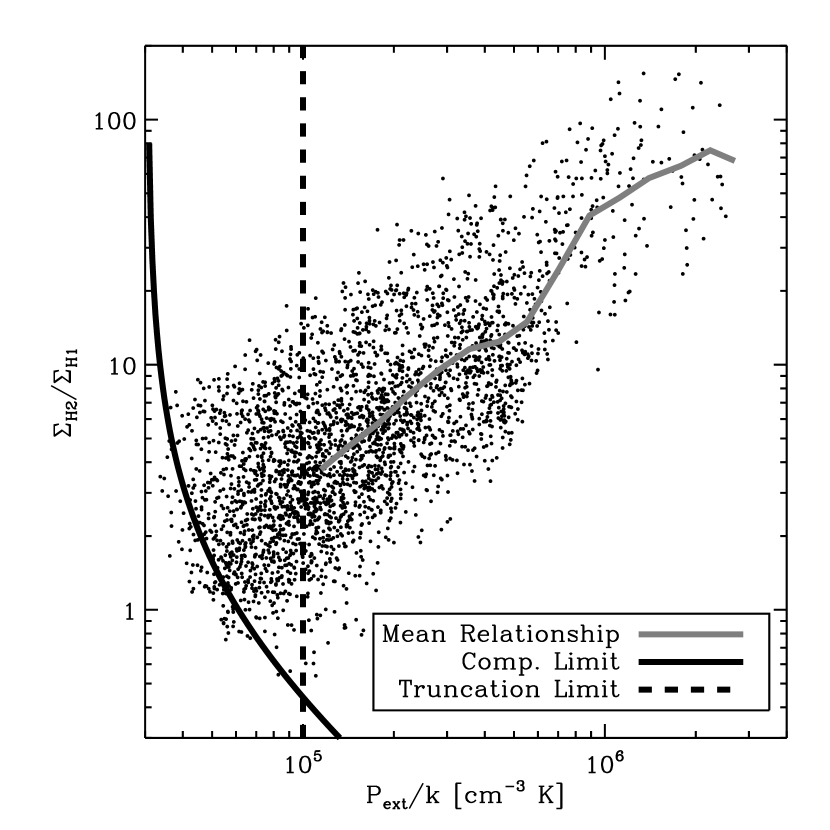
Figure 1.— Molecular gas fraction as a function of midplane hydrostatic pressure for NGC 5194 (M51). The mean relationship is plotted in a thick gray line. The completeness limit arising from the molecular gas observations is plotted as a solid black line. The intersection of this line with the bottom of the observed distribution determines the truncation limit. The relationship between $P_{ext}$ and $R_{mol}$ is only calculated above this limit.

3.3. Completeness

We calculate $R_{mol}$ as a function of pressure on a pixel-by-pixel basis for all pixels that have measured surface densities of H I, CO, and 2 $\mu$m emission. Figure 1 is a plot of the correlation between these two quantities for NGC 5194 (M51). The two quantities are clearly correlated, but the different signal-to-noise ratios of the three data sets affect the distribution of points in the Figure. Of the three tracers, the CO emission has the lowest signal-to-noise, and is found at the fewest positions. It is thus the limiting factor in our analysis.

To illustrate the effects of finite sensitivity, we plot the locus of points where $\Sigma_{\mathrm{H2}}=8~{}M_{\odot}~{}\mbox{pc}^{-2}$ (the 5$\sigma$ sensitivity limit), $\Sigma_{\star}=300~{}M_{\odot}~{}\mbox{pc}^{-2}$, and a range of $\Sigma_{\mathrm{HI}}$ as the solid curve in Figure 1. We choose $\Sigma_{\star}=300~{}M_{\odot}~{}\mbox{pc}^{-2}$, so that the curve roughly coincides with the left boundary of the data. The curve is a good match to the shape of the left edge of the data in Figure 1. At a given pressure, points that lie below the line have CO surface brightnesses that are too weak to be detected; the solid line therefore represents the completeness limit for the observations. Because we wish to bin the data in values of $P_{ext}$, we have complete CO data only when the lowest measured values of $R_{mol}$ for the entire sample lie above the completeness line. Thus all of the data to the right of the dotted line, the intersection of the completeness line with the lowest values of $R_{mol}$ have complete CO data (i.e. complete measured values of $\Sigma_{\mathrm{H2}}$). Plots of $P_{ext}$ vs. $R_{mol}$ for four other representative galaxies are shown in Figure 2, showing that the scatter of the individual points within a galaxy exhibits considerable variation.

Figure 2.— Plots of $P_{ext}$ vs. $R_{mol}$ for four galaxies showing a range of scatter on a pixel-by-pixel basis. For galaxies such as NGC 3521, the scatter is so small (15%) that finding the completeness limit is trivial. For galaxies such as NGC 7331, we must use the technique described in the text for estimating the completeness limits in the relationship.

3.4. The Relationship Between $P_{ext}$ and $R_{mol}$

Since we wish to measure the molecular gas fraction as a function of $P_{ext}/k$, we average $R_{mol}$ in bins of 0.1 dex in $P_{ext}/k$. To avoid biases due to the finite sensitivity, the analysis is restricted to $P_{ext}/k$ larger than $P_{min}/k$, the value where the completeness curve intersects the bottom of the data distribution. Practically, we define $P_{min}/k$ as the bin containing the minimum value of $R_{mol}$ in the sample, and only consider bins of $P_{ext}/k$ with this value and larger. Since the upper limits on the CO surface brightness affect both $P_{ext}$ and $R_{mol}$, points without identifiable CO emission provide little additional information, and we discard these data from our analysis. The uncertainty in $\log R_{mol}$ ($\delta\log R_{mol}$) is determined by the standard deviation of points in each bin ($\sigma_{\log R_{mol}}$) divided by the square root of the number of independent samples in each bin:

$$\delta\log R_{mol}\equiv\frac{\sigma_{\log R_{mol}}}{\sqrt{N/n_{beam}}},$$ (10)

where $N$ is the number of pixels contributing to each bin and $n_{beam}$ is the number of pixels per independent beam.

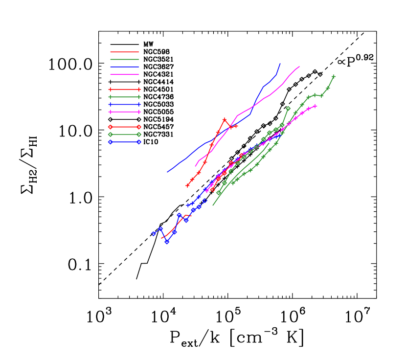
Figure 3.— Molecular gas fraction as a function of midplane hydrostatic pressure for 14 galaxies. All galaxies follow a similar scaling between $P_{ext}$ and $R_{mol}$. The mean index of the relationship is $0.92\pm 0.07$ (dashed line). There are two categories of galaxies, offset from each other by a factor of 5 in $P_{0}$.

Table 2Results of Pressure Analysis

Galaxy	$\alpha$	$P_{0}/k$	Scatter	$\langle\Sigma_{\mathrm{HI}}\cos i\rangle$	Morphological
Name		($10^{4}$ cm-3 K)		($M_{\odot}~{}\mbox{pc}^{-2}$)	class
MW	$1.64\pm 0.11$	2.0	0.09	8.4	Sb
NGC 598	$0.87\pm 0.14$	5.1	0.03	9.3	SA(s)cd
NGC 3521	$1.02\pm 0.03$	7.1	0.02	16.8	SAB(rs)bc
NGC 3627	$0.81\pm 0.03$	0.4	0.10	4.3	SAB(s)b
NGC 4321	$0.84\pm 0.03$	0.7	0.06	6.7	SAB(s)bc
NGC 4414	$0.89\pm 0.02$	4.6	0.02	14.4	SA(rs)c?
NGC 4501	$1.07\pm 0.08$	1.2	0.13	4.2	SA(rs)b
NGC 4736	$0.93\pm 0.04$	6.5	0.09	11.1	(R)SA(r)ab
NGC 5033	$0.76\pm 0.03$	3.0	0.05	11.5	SA(s)c
NGC 5055	$0.73\pm 0.02$	2.8	0.03	11.5	SA(rs)bc
NGC 5194	$1.00\pm 0.05$	3.0	0.07	13.2	SA(s)bc pec
NGC 5457	$0.58\pm 0.32$	2.1	0.09	16.6	SAB(rs)cd
NGC 7331	$1.01\pm 0.06$	5.1	0.05	14.5	SA(s)b
IC 10	$0.73\pm 0.14$	5.6	0.10	6.4	dIrr IV/BCD
Mean	$0.92\pm 0.07$	3.5	0.06	10.6	Sbc
Mean (Non-interacting)	$0.92\pm 0.10$	4.3	0.05	12.2	Sbc
Combined Data	$0.94\pm 0.02$	4.5	0.14	9.9	$\cdots$

We plot the relationship between hydrostatic pressure and molecular gas fraction in Figure 3. The figure shows that a power law is a good representation of the functional form between the two quantities. The plots for the individual galaxies have a similar slope but seem to lie in two groups. We fit a linear relationship between $\log(P_{ext}/k)$ and $\log R_{mol}$ to estimate the parameters for a power-law relationship between the two variables:

$$R_{mol}=\left(\frac{P_{ext}}{P_{0}}\right)^{\alpha}$$ (11)

The derived values of the index $\alpha$ are reported in Table 2 with uncertainties generated by bootstrapping. $P_{0}$ is the external pressure in the ISM when the molecular fraction is unity. The results for all of the galaxies is given by:

$$R_{mol}=\left[\frac{P_{ext}/k}{(3.5\pm 0.6)\times 10^{4}}\right]^{0.92\pm 0.07}.$$ (12)

The data for NGC 3627, NGC 4321, and NGC 4501 lie significantly above the data for the remainder of the sample. Splitting the data into two groups, we find $\langle P_{0}/k\rangle=7700\mbox{ cm}^{-3}~{}\mbox{K}$ for these three galaxies but $\langle P_{0}/k\rangle=43000\mbox{ cm}^{-3}~{}\mbox{K}$ for the remainder of the sample. However, the mean index, $\langle\alpha\rangle$, for each of the subsets is indistinguishable from that of the sample as a whole. The difference between the two populations can be attributed to differences in the H I content of the disks. In Table 2, we also tabulate the median values of $\Sigma_{\mathrm{HI}}\cos i$ used in the analysis. We note that $\langle\Sigma_{\mathrm{HI}}\cos i\rangle$ is significantly lower for these three galaxies than for the remainder of the systems. The low values of $\Sigma_{\mathrm{HI}}\cos i$ likely arise from ram pressure or tidal stripping in these galaxies. The other galaxies in our sample appear to be field galaxies without significant tidal or ram pressure interactions. NGC 3627 is in the Leo Triplet of galaxies and has had a recent interaction with NGC 3628, evidenced by the asymmetric H I distribution in NGC 3627 and the long tail of H I from NGC 3628 (Haynes et al., 1979). NGC 4321 and NGC 4501 are both members of the Virgo Cluster and are known to be H I poor from previous work (Giovanelli & Haynes, 1983). The H I morphology of NGC 4501 shows ample evidence that the galaxy is undergoing ram pressure stripping in the high-pressure cluster environment. NGC 4321 is less obviously disturbed, but still H I poor. The three galaxies do not appear to be discrepant in any other way.

If we remove these galaxies from the mean relationship, we obtain:

$$R_{mol}=\left[\frac{P_{ext}/k}{(4.3\pm 0.6)\times 10^{4}}\right]^{0.92\pm 0.10},$$ (13)

which changes $P_{0}$ by only 20%. This may be a more representative relationship than Equation 12 because the discrepant galaxies may be subject to pressure in addition to the hydrostatic pressure, which would move them to the right in Figure 3. We also fit a power law to the combined data for the non-interacting galaxies, rather than fitting each galaxy and then averaging (Figure 4). This weights the fits by the total number of data at a given $P_{ext}$. Because the nearby, H I-rich galaxies (IC10, M33) have many more independent samples, this fit emphasizes galaxies with low values of $R_{mol}$. Nonetheless, the resulting fit (Combined Data in Table 2) is indistinguishable from the average of the individual fits to the non-interacting data.

It is worth noting that although we derive a relationship involving the gas pressure, because we take the velocity dispersion of the gas as constant, and because the turbulent pressure, $\rho v^{2}$, provides most of the support of the gas layer, our expression is essentially equivalent to $R_{mol}$ being a function of the midplane gas density. We cannot, with our data alone, decide between these two possibilities. But using the equivalent density parameterization yields a true Schmidt law, where the star formation rate is dependent on ISM density (Schmidt, 1959).

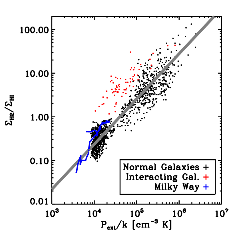
Figure 4.— Molecular gas fraction as a function of midplane hydrostatic pressure for all data in the sample. Each point represents an independent measurement of $\Sigma_{\mathrm{HI}}$, $\Sigma_{\mathrm{H2}}$ and $\Sigma_{\star}$. A linear fit to $\log R_{mol}$ vs. $\log P_{ext}/k$ is shown as a thick gray line. The data for the interacting galaxies (red, NGC 3627, NGC 4321, NGC 4501) are excluded from the fit. The results are indistinguishable from determining the relationship between $R_{mol}$ and $P_{ext}$ for each galaxy individually.

3.5. Comparison with Previous Work

Wong & Blitz (2002) found, for a sample of seven galaxies, that $R_{mol}$ $\propto{P_{ext}}^{0.8}$ over one and a half orders of magnitude in pressure. For a given $R_{mol}$, $P_{ext}$ ranges over an order of magnitude suggesting that the dispersion in the pressure is about a factor of 2 – 3. We have made several improvements to the Wong & Blitz (2002) analysis as follows. Rather than taking azimuthal averages, we have calculated $R_{mol}$ and $P_{ext}$ on a pixel-by-pixel basis. Wong & Blitz (2002) used an expression for the pressure by Elmegreen (1993) that requires knowledge of the stellar velocity dispersion in disks, a quantity that is difficult to measure, and one that is expected to vary significantly as a function of radius. In this paper, we use a different, but equivalent expression that relates the pressure to the stellar surface density and stellar scale height (BR04). The surface density is observable; the scale height varies little within galaxies and its value can be inferred from the observable scale length (Kregel et al., 2002, Equation 9). By including additional galaxies, we are able to extend Wong & Blitz (2002) to a total of three orders of magnitude and to include lower mass and lower metallicity galaxies. Our method also significantly reduces the scatter among the galaxies, measured by the dispersion of the values of $P_{0}/k$ in Table 2.

We note that over the range of galactic radius for M33 included in our sample, there is a decrease in the metallicity by a factor of 6 (Henry & Howard, 1995). Although the range of pressure sampled in M33 is small, there is no systematic offset from the mean relation shown in Figure 3 with metallicity. The same is true for IC10, which has a metallicity 1/5 solar (Garnett, 1990).

On theoretical grounds, Elmegreen (1993) derives a much steeper dependence of $R_{mol}$ on pressure than we do, but he also includes a dependence on the emissivity of the dissociating radiation field, $j$. Wong & Blitz (2002) found that if one assumes that $j\propto\Sigma_{gas}\propto\Sigma_{\star}$, Elmegreen’s (1993) expression is equivalent to $f_{mol}={\Sigma_{\mathrm{H2}}}/{{\Sigma_{g}}}\propto{P_{ext}}^{1.7}$. However, Wong & Blitz (2002) did not take into account that $c_{\star}$, the velocity dispersion of the stars, has a radial dependence on $\Sigma_{\star}$, which is approximately $\propto{\Sigma_{\star}}^{0.5}$. By ignoring the gravity of the gas as we have done in equation 2, and including the dependence of $c_{\star}$ on ${\Sigma_{\star}},$ Elmegreen’s expression for $P$, has the same functional dependencies as ours. In the regime of low $f_{mol}$ , where Elmegreen’s treatment is meant to be appropriate, $f_{mol}\simeq R_{mol}$. Although $j$ probably does not have a simple power law dependence on $\Sigma_{gas}$, if it can be approximated as $j\propto{\Sigma_{g}}$, then Elmegreen’s (1993) expression for $f_{mol}$ has a power law dependence quite close to what we find observationally.

We note further that although one expects $R_{mol}$ to have a dependence on $j$ on physical grounds, the small scatter of the lines in Figure 3 implies that empirically, $R_{mol}$ behaves as if it depends on pressure only. The discussion above suggests that the dependence on $j$ is subsumed within the empirical relationship.

3.6. Notes on Individual Galaxies

The Milky Way – For the Galaxy, we use the values of Dame (1993) for $\Sigma_{\mathrm{HI}}$ and $\Sigma_{\mathrm{H2}}$ at $R_{gal}>3$ kpc. We assume that the local stellar surface density in the vicinity of the Sun is 35 $M_{\odot}$ pc^-2 and that the stars are distributed in an exponential disk with scale length 3 kpc (Dehnen & Binney, 1998) with $R_{0}=8.0$ kpc. We scale $\Sigma_{\mathrm{H2}}$ by 1.36 to account for the presence of helium and by (2/2.3) to account for the different conversion factor adopted in that study. Finally, we scale $\Sigma_{\mathrm{HI}}$ by 1.5 to account for the presence of high latitude gas, based on the results beyond the Solar circle from Levine et al. (2006).

NGC 598 (M33) – NGC 598 is the closest extragalactic source in our sample. The disk of NGC 598 is stable according to the Toomre criterion (Martin & Kennicutt, 2001), making it a notable test case for for comparing the role of gravitational instability with that of pressure in regulating the ISM and star formation. We generated a molecular gas map from a masked integrated-intensity map from the FCRAO 14-m survey of the galaxy (Heyer et al., 2004). Apart from the Milky Way, it is the only other disk galaxy in the sample with sufficient surface brightness sensitivity in the CO map to measure $R_{mol}$ where $R_{mol}<1$. The derived index of $\alpha=0.87$ can be compared to the work of Heyer et al. (2004) who show that $R_{mol}\propto P_{ext}^{2.3}j^{-1}$ where $j$ is the mean radiation field. Using $j\propto\Sigma_{\star}$, we reproduce their index to the pressure relationship. Performing a similar analysis for the remainder of our sample finds indices ranging from 1.4 to 2.3.

NGC 3627 – This galaxy is a molecule rich member of the Leo Triplet and the ISM of the galaxy has been affected by interaction with the remainder of the group. NGC 3628, another member of the triplet, is also very molecule rich (Young et al., 1995). The interactions between the three galaxies have stripped a long plume of material from NGC 3628 and have also likely depleted the H I in the disk of NGC 3627.

NGC 4321 (M100) – This galaxy is a member of the Virgo cluster, but is not obviously undergoing ram pressure stripping at the present time. Azimuthally averaging the H I data shows a slight downturn at large radii, and the median surface density for the H I is relatively high (6.7 $M_{\odot}~{}\mbox{pc}^{-2}$) compared to the other interacting galaxies in our sample (NGC 3627 and NGC 4501). Of the three galaxies undergoing interactions, this galaxy appears to be the least affected by interaction. However, it is noticeably deficient in H I with a total atomic gas mass a factor of three lower than comparable field galaxies (Kenney & Young, 1989).

NGC 4501 (M88) – We used archival BIMA data from NGC 4501 to generate the CO map of NGC 4501 used in this study. The data were originally presented in Wong & Blitz (2002). NGC 4501 is a member of the Virgo Cluster and its H I morphology appears to be noticeably affected by the cluster environment. It is separated by $\sim 500$ kpc on the plane of the sky from M87; and the H I surface density is asymmetrical, apparently piled up on the side of the galaxy closest to M87 (Cayatte et al., 1990). The cluster environment appears to be responsible for the depletion of the atomic gas which is a factor of 3 lower than what would be expected from a field spiral of similar stellar mass (Kenney & Young, 1989).

NGC 4736 (M94) – This galaxy has the earliest morphological type in our sample and sizable amounts of neutral gas are found within the bulge of the galaxy. The pressure formulae used in this paper is appropriate for the disks of galaxies, but should be an upper limit for the bulges of galaxies, since the thickness of bulges is larger than disks. Applying the pressure formulae for disks to NGC 4736 may account for the high value of $P_{0}$ in the system.

NGC 5194 (M51a) – NGC 5194 is a classic example of grand-design spiral structure in galaxies. The high resolution observations of NGC 5194 facilitate the measurement of $P_{ext}$ and $R_{mol}$ both in and out of the spiral arms seen in the ISM. In both the arms and the interarm regions, $P_{ext}$ appears to be a good predictor of $R_{mol}$.

NGC 5457 (M101) – The overlap between H I and CO detections spans only a very small portion of the galaxy. The H I surface density drops markedly in the center of the galaxy where the molecular gas is concentrated (Wong & Blitz, 2002). In the small overlap region, however, the data from NGC 5457 agree well with the remainder of sample.

IC 10 – We include IC 10 in our sample to investigate the $R_{mol}$ vs. $P_{ext}$ relationship in a low metallicity environment. The gas geometry of the system is quite complex and not apparently confined to the stellar disk, which may affect the applicability of Equation 5. However, Leroy et al. (2006) noted that the molecular gas in the system tended to be found on filaments of atomic gas that were coincident with the stellar disk of the galaxy. We include the pressure data from their work in this study. They assume a characteristic scale height of the stellar component of 300 pc. We correct the surface densities of gas by the inclination of the stellar disk assuming that the gas spatially coincident with the stellar disk actually lies within the disk.

3.7. Systematic Effects

In this section, we discuss how variations in our assumptions and interpretations affect the results.

Since $\Sigma_{\mathrm{H2}}$ appears in the expressions for both $R_{mol}$ and $P_{ext}$, it is possible that some of the observed correlation in Figure 3 arises simply because we are correlating CO emission with itself. As we can see from Figure 4, however, most of our individual data points come from the low pressure regime ($P<P_{0}$), where no such correlation is expected. Thus, this concern is most important where $R_{mol}\gg 1$. In that case, the Equation 3, as plotted in Figure 3 reduces to:

$${\rm log}\Sigma_{\mathrm{H2}}-{\rm log}\Sigma_{\mathrm{HI}}=\alpha~{}{\rm log}\Sigma_{\mathrm{H2}}+\frac{\alpha}{2}~{}{\rm log}\Sigma_{\star}+const.$$ (14)

where $\alpha$ is the quantity we are trying to determine (assuming that $R_{mol}$ is proportional to $P^{\alpha}$). Since $\Sigma_{\mathrm{HI}}$ shows little variation compared to either $\Sigma_{\mathrm{H2}}$ or $\Sigma_{\star}$, and because log $\Sigma_{\mathrm{H2}}$ dominates the left hand side of Equation 14 for large $R_{mol}$, we can absorb log $\Sigma_{\mathrm{HI}}$ into the constant. Because log $\Sigma_{\mathrm{H2}}$ appears on both sides of Equation 14, at least some of the correlation at $R_{mol}\gtrsim 5$ is due to correlating log $\Sigma_{\mathrm{H2}}$ with itself. The slope of the $P-R_{mol}$ relationship is given by:

$$\alpha=\frac{\log\Sigma_{\mathrm{H2}}+const.}{\log\Sigma_{\mathrm{H2}}+(\log\Sigma_{\star})/2}$$ (15)

As long as the range of values of $(\log\Sigma_{\star})/2$ are comparable to the range of values of $\log\Sigma_{\mathrm{H2}}$, as is the case for most of the data presented in Figure 3, both terms in the denominator will determine the slope, and thus the value of $\alpha$. Thus, even for large values of $R_{mol}$, where some of the correlation in the $P-R_{mol}$ relation is produced by $\Sigma_{\mathrm{H2}}$ appearing on both axes, the data still provide information about the functional form of Equation 3.

To estimate the amount of correlation that arises purely from the mathematical construction of our analysis, we recalculate $R_{mol}$ and $P_{ext}$ after scrambling the original measurements of $\Sigma_{\mathrm{HI}},\Sigma_{\mathrm{H2}}$ and $\Sigma_{\star}$. This randomization retains the original data but the surface density measurements for each disk component no longer correspond to the values of the other components. Using the scrambled data for $R_{mol}$ and $P_{ext}$ we do indeed find a significant correlation in the randomized data, particularly evident at $R_{mol}\gtrsim 2$. The power-law index for the scrambled data is $\alpha=1.5\pm 0.02$, significantly greater than the derived relationship for the real data. We conclude that we are observing a physically significant relationship although we recognize that the data for $R_{mol}\gtrsim 2$ would not be compelling on their own. When used in conjunction with the data for low values of $R_{mol}$, however, the molecule-rich regions of galaxies extend the trend into high-pressure regions.

Another concern is that variations in the CO-to-H₂ conversion factor may substantially alter our results. However, the only regions included in this sample that show good evidence for variations in the CO-to-H₂ conversion factor that are also included in this sample are the molecule rich regions in the central $\sim 200$ pc of galaxies (e.g. Meier & Turner, 2004). In these regions, $R_{mol}\gg 2$ and the observed correlation is largely the product of correlating CO emission with itself. As a result, changes in the CO-to-H₂ conversion factor will alter $R_{mol}$ and $P_{ext}$ by roughly the same amount and the data will likely remain consistent with the observed trend. Thus, variations in the conversion factor are unlikely to substantially affect our results.

The projected resolution at the distance of the galaxies varies by nearly an order of magnitude across the sample. There is no significant correlation between physical resolution and the index of the derived relationship or the degree of scatter around the mean trend. To assess the effect of the physical resolution on our results, we repeat the analysis, convolving the data to a constant physical resolution of 1.8 kpc. This degrades the resolution to a constant scale for all galaxies except for NGC 5033. We find no significant change in the results as a result of smoothing to this resolution. We conclude that resolution effects do not affect the results significantly.

The assumption of a constant velocity dispersion is well-justified (van der Kruit & Shostak, 1982; Shostak & van der Kruit, 1984; van der Kruit & Shostak, 1984; van Zee & Bryant, 1999), but there are $\sim 30\%$ variations in velocity dispersion within and among galaxies. These differences may account for the offsets and scatter seen in Figure 3.

4. Discussion

In nearby galaxies where the dominant state of the gas is atomic, the atomic gas occurs primarily in filaments (Kim et al., 1998; Engargiola et al., 2003; Leroy et al., 2006), and the formation of the filaments appears to precede the formation of the molecular gas (Blitz et al., 2006). From §3 and BR04, we have shown that hydrostatic pressure alone is sufficient to determine what fraction of the neutral gas at any location in a galaxy is molecular, and we have determined the quantitative relationship between pressure and molecular gas fraction. We have not been able to show, however, how the molecular gas collects itself into GMCs, or even if the atomic gas first collects itself into GMC-sized objects and then becomes molecular. This detail may not be important for determining the star formation rates in galaxies on kiloparsec scales, since the rate at which stars form from the molecular gas appears to be well determined on scales larger than a GMC (Wong & Blitz, 2002), but is relevant to issues related to the stability of the ISM.

In all of the galaxies we have examined in this paper, pressure is measured on a scale large compared to the size of a GMC, because of either the relatively poor resolution of the H I observations, or because the galaxies are relatively distant. We expect that Equation 13 would break down on a scale comparable to that of a typical GMC because the pressure within a GMC is enhanced by its self-gravity and is no longer in pressure equilibrium with its environment. We would guess that the scale on which the relation is valid is about equal to twice a pressure scale height ($\sim$ 400 pc in the solar vicinity of the Milky Way). The pressure will be in equilibrium on such a vertical scale, on average, and is unlikely to vary by very much on a similar scale in the galactic plane.

4.1. Applicability to Other Kinds of Galaxies

Our sample of galaxies is limited to normal spirals and some dwarf galaxies. It contains weak Seyferts and galaxies with low level starbursts and galaxies with metallicities that range from solar values to values as low as 1/6 solar (IC 10). It does not include elliptical galaxies, and S0s, a number of which have been shown to be molecule rich (Young, 2002; Young et al., 1995), nor does it include very low metallicity dwarfs such as I Zw 18, luminous starbursts, strong Seyferts or merging systems. Equation 13 may not be applicable in these systems, but the pressure in the ISM can be estimated from other means. Equation 13 uses an equilibrium approximation of disk structure to estimate $\rho{v_{g}}^{2}$, a quantity that can be determined equally well using a variety of methods. In elliptical galaxies, the pressure may be measured directly from density and temperature information inferred from x-ray data. In the bulges of disk galaxies, other constraints from stellar velocity dispersions and scale heights can be used to estimate a more accurate stellar mass distribution. Programs are underway to to probe the relationship between molecular gas fraction and ISM pressure in an array of such systems. The Large and Small Magellanic Clouds will also be good testbeds for determining the general applicability of the pressure-molecular fraction relation. In these two systems with irregular morphologies, we can measure the relationship between molecular gas fraction and pressure at high resolution.

Galaxies with low metallicities are interesting regions in which to study the molecular fraction of the ISM. In these systems, the flux of dissociating UV photons tends to be higher than in the disk galaxies that we studied in this sample. In conjunction with the volume density of hydrogen, the UV flux establishes the equilibrium molecular fraction in the ISM of the neutral gas. Hence, we suspect systems with low metallicity and high UV flux (such as the SMC) may be significantly offset from the $R_{mol}$ – $P_{ext}$ relationship seen for disk galaxies with approximately solar metallicity.

4.2. Molecular Gas and Star Formation

Kennicutt (1998, hereafter K98) has argued that the surface density of the rate of star formation $\Sigma_{\mathrm{SFR}}$ is proportional to the sum of the atomic and molecular gas surface density, $\Sigma_{g}$ over a wide range of galaxy luminosity. This relationship is puzzling because stars form only from molecular gas. K98 cites the relative tightness of his plot of $\Sigma_{\mathrm{SFR}}$ vs. $\Sigma_{g}$ compared to his plot of $\Sigma_{\mathrm{SFR}}$ vs. $\Sigma_{\mathrm{H2}}$. However, when averaged over kiloparsec scales, $\Sigma_{\mathrm{HI}}$ tends to saturate at a value of $\sim$10 $M_{\sun}$ pc^-2, or about $1.3\times 10^{21}$ cm^-2 (e.g.  Cayatte et al., 1994; Wong & Blitz, 2002), the relationship between $\Sigma_{\mathrm{SFR}}$ and $\Sigma_{\mathrm{HI}}$ in K98 is less a correlation than a plot showing the saturation of the H I line.

Wong & Blitz (2002, hereafter WB02), on the other hand, have shown that for 7 well-studied galaxies in the BIMA SONG CO survey, (Helfer et al., 2003), the proportionality found by K98 does indeed hold, but for the molecular gas only. That is, K98 finds that $\Sigma_{\mathrm{SFR}}=0.16\ \Sigma_{g}^{1.4}$, where $\Sigma_{\mathrm{SFR}}$ is measured in $M_{\sun}$ pc^-2 Gyr^-1 and ${\Sigma_{g}}$ is measured in $M_{\sun}$ pc^-2. WB02 find that $\Sigma_{\mathrm{SFR}}=0.13\ \Sigma_{\mathrm{H2}}^{1.4}$. These relations use values of $X_{\mathrm{CO}}$ that differ in whether or not they include a correction for helium. If helium is included in the WB02 relation, then their coefficient is 0.18 rather than 0.13, which differs from the K98 value by only 13%. This is not entirely surprising, since WB02 use K98’s calibration of H$\alpha$ line strength vs. star formation rate.

Murgia et al. (2002) developed a star formation formulation based on radio continuum measurements calibrated to the supernova rate in a number of galaxies (Condon, 1992), This relation, like WB02, relates the star formation rate to $\Sigma_{\mathrm{H2}}$ and finds a power-law index of 1.3, indistinguishable from 1.4 within the uncertainties. The Murgia et al. (2002) coefficient of proportionality is a bit higher: 0.26 rather than 0.18, but uses the Miller & Scalo (1979) IMF rather than a Salpeter (1955) IMF between 0.1 and 100 $M_{\sun}$. Murgia et al. (2002) do not give a lower mass limit, but the differences between the two IMFs could make up much of the discrepancy in the coefficient.

The K98 relation is based primarily on global averages, and the relation of WB02 is based on pixel-by-pixel measurements convolved to the same linear resolution. As a practical matter, the differences between these formulations are unimportant for regions of galaxies where the ISM is dominated by molecular gas, such as galactic centers, as well as most of the regions of galaxies over which BIMA SONG has enough sensitivity to detect CO. However, throughout the entire disk of the Milky Way, $\Sigma_{\mathrm{HI}}\geq\Sigma_{\mathrm{H2}}$ (except for the central 300 pc; Dame, 1993), as is also the case in M33 (Heyer et al., 2004) and most of M31 (Nieten et al., 2006). In general, the interstellar medium in dwarf galaxies is dominated by H I rather than molecular gas, and it is in M33 and in dwarf galaxies that Martin & Kennicutt (2001) find that their star formation prescription breaks down. Observations of H I rich dwarf galaxies should be a good test of whether the K98 or WB02 relation is better at predicting the star formation rate. One recent study has been completed by Heyer et al. (2004) on the Kennicutt-Schmidt law in M33 where they find $\Sigma_{\mathrm{SFR}}\propto\Sigma_{\mathrm{H2}}^{1.36}$ in good agreement with the work of WB02 and Murgia et al. (2002). When they include atomic gas in their analysis, they find $\Sigma_{\mathrm{SFR}}\propto\Sigma_{\mathrm{H2}}^{3.3}$, differing dramatically from the results of K98.

4.2.1 CO, HCN, FIR and Star Formation

In her ground breaking work on the relationship between dense gas and star formation, Lada (1992) showed that in the Orion B molecular cloud (L1630), nearly all of the star formation is associated with the H₂ traced by the CS molecule, a tracer of dense molecular gas. Most of the molecular gas in L1630 traced by CO, a moderate density tracer, is inert and does not take part in the star formation process. Why, then, is there a good relationship between $\Sigma_{\mathrm{CO}}$ and star formation if the molecular gas traced by CO has little direct bearing on star formation?

The work of Gao & Solomon (2004, hereafter GS04) and of Wu et al. (2005) suggests an answer. GS04 show that HCN is a linear tracer of the star formation rate in luminous and ultraluminous galaxies while CO is not. In their work, the star formation rate is determined from the far IR luminosity. The connection to Lada’s (1992) work is that both HCN and CS are good tracers of dense gas with $n(\mbox{H${}_{2}$})\sim 10^{4-5}$, but HCN is somewhat more luminous, on average, in galaxies (Helfer & Blitz, 1997b, and references therein). The GS04 plots of the correlation between HCN and CO with IR luminosity show what appear to be comparably good fits to the data, though the fit using CO is not linear, while the fit using HCN is. The correlation coefficients for both fits are quite high, but the fit using HCN is marginally better than for CO ($R=0.94$ vs. 0.88), and the scatter somewhat less (0.25 dex vs. 0.35 dex). In luminous and ultra-luminous infrared galaxies, GS04 find that the HCN luminosity is related to the CO luminosity: $L_{\mathrm{HCN}}=1.6\times 10^{-5}~{}L_{\mathrm{CO}}^{1.38}$ for $L$ measured in K km s^-1 pc².

Wu et al. (2005) show that the linearity between the HCN and IR luminosity continues down to the scale of individual dense cores in Galactic molecular clouds, implying that the HCN – IR relationship for starbursts continues down to the level of star-forming clumps. The linearity holds over a total range of luminosity of 7 – 8 orders of magnitude. Correlations using luminosity usually look remarkably good because one is correlating distance (squared) with itself on both axes, making the correlation much more striking than it actually is. A better comparison is between distance independent quantities such as surface brightness. Nevertheless, there seems to be good evidence that the linearity of IR luminosity with HCN line strength is quite good for a range of objects from individual Galactic GMCs to ULIRGs.

4.2.2 A Pressure-Based Prescription for Star Formation on Galactic Scales

We propose an alternative, pressure-based prescription for galaxy-scale star formation centering on three empirically-derived relationships. First, we assume that the FIR luminosity is a good tracer of the massive star formation in a galaxy because the FIR emission is proportional to the number of Lyman continuum photons, nearly all of which are absorbed by dust, From GS04 (and references therein),

$$\dot{M}_{\mathrm{SFR}} \approx 2\times 10^{-10}~{}(L_{\mathrm{FIR}}/L_{\sun})~{}~{}M_{\sun}~{}\mbox{yr}^{-1},~{}\mbox{and}$$ (16)

$$M_{\mathrm{dense}} = 14~{}\left(\frac{L_{\mathrm{HCN}}}{\mbox{K km s}^{-1}\mbox{ pc}^{2}}\right)~{}~{}M_{\sun}$$ (17)

Next, we assume that all star formation takes place in dense molecular gas which has a constant star formation efficiency. Expressing this in a form comparable to that of K98 using the above notation gives:

$$\Sigma_{\mathrm{SFR}}=\epsilon\Sigma_{\mathrm{H2}}(\mathrm{HCN})$$ (18)

GS04 and Wu et al. (2005) measure $\epsilon\approx 10-13\mbox{ Gyr}^{-1}$. Expressing Equation 18 in terms of the total molecular gas traced by CO gives:

$$\Sigma_{\mathrm{SFR}}=\epsilon\Sigma_{\mathrm{H2}}({\mathrm{CO}})\left[\frac{\Sigma_{\mathrm{H2}}(\mathrm{HCN})}{\Sigma_{\mathrm{H2}}(\mathrm{CO})}\right]$$ (19)

which is related to the total gas content:

$$\Sigma_{\mathrm{SFR}}=\epsilon\Sigma_{g}f_{mol}\left[\frac{\Sigma_{\mathrm{H2}}(\mathrm{HCN})}{\Sigma_{\mathrm{H2}}(\mathrm{CO})}\right]$$ (20)

where $f_{mol}=\Sigma_{\mathrm{H2}}/{\Sigma_{g}}=R_{mol}/(R_{mol}+1)$ and $R_{mol}=\Sigma_{\mathrm{H2}}/\Sigma_{\mathrm{HI}}.$ Third, we assume that $f_{mol}$ is determined from the pressure and the total amount of gas present, and can be calculated from Equations  11 and 12 . We can rewrite Equation 11:

$$f_{mol}=\frac{R_{mol}}{(R_{mol}+1)}=\left[1+\left(\frac{P_{ext}}{P_{0}}\right)^{-\alpha}\right]^{-1}.$$ (21)

For an integrated intensity, $I$, expressed in units of K km s^-1 and $\Sigma$ measured in $M_{\sun}~{}\mbox{pc}^{-2}$, $\Sigma_{\mathrm{H2}}(\mathrm{HCN})=14~{}I(\mathrm{HCN})$ (GS04), and $\Sigma_{\mathrm{H2}}(\mathrm{CO})=4.4~{}I(\mathrm{CO})$ for our adopted CO-to-H₂ conversion factor (§3.2) corrected for helium. Thus,

$$\frac{\Sigma_{\mathrm{H2}}(\mathrm{HCN})}{\Sigma_{\mathrm{H2}}(\mathrm{CO})}=3.2\frac{I(\mathrm{HCN})}{I(\mathrm{CO})}$$ (22)

Unlike theoretical explanations of the Kennicutt-Schmidt law (e.g.  Krumholz & McKee, 2005), this formulation separates the empirical star formation relationship of K98 into three constituent empirical relationships. The ability to reproduce the K98 results should not be surprising – all three of the constituent relationships are based on galaxies similar to those in K98. A consistent constant of proportionality is an indication of accurate calibration of the various quantities involved. What is notable about this formulation is the ability to characterize star formation on a galactic scale using the star formation efficiency of dense gas and the role of pressure in determining both the fraction of gas that is molecular and the fraction of that molecular gas that is dense enough to form stars.

The Low Pressure Regime

Except for the central 300 pc of the Milky Way, and the inner regions of M31, the mean H I surface density exceeds that of the H₂ when averaged over several hundred pc everywhere in each galaxy. Thus, most of the molecular gas in these galaxies occurs in the regime where $P_{0}>P_{ext}$. For most GMCs in Local Group galaxies, the surface density of GMCs as traced by CO is roughly constant with a value of $\sim 100~{}M_{\sun}~{}\mbox{pc}^{-2}$ (Blitz et al., 2006), so the fraction of dense gas and consequently, the star formation rate of individual GMCs, will also be roughly constant, as is observed (Mooney & Solomon, 1988; Scoville & Good, 1989). Variations in $\Sigma_{\mathrm{SFR}}$ over kiloparsec scales thus result from changes in the fraction of neutral gas bound up in GMCs ($\propto f_{mol}$). That is, averaging emission on large enough scales ($\gtrsim$ 200 pc) over which the surface filling fraction of molecular gas is small, pushes the Kennicutt-Schmidt law into the regime of small values of $\Sigma_{\mathrm{H2}}$ since averaging GMCs with atomic gas that has no star formation will geometrically dilute both $\Sigma_{\mathrm{SFR}}$ and $\Sigma_{\mathrm{H2}}(\mathrm{CO})$ by a comparable, though not identical, factor.

In this regime, we may take Equation 22 to be constant. Helfer & Blitz (1997a) derive a value of 0.026 $\pm 0.008$ for the ratio of integrated intensities averaged over the inner disk of the Milky Way. Similarly, GS04 find $L(\mathrm{HCN})/L(\mathrm{CO})=0.039$ for their low-luminosity galaxies. We adopt the average of these two values as a characteristic line ratio which implies that the ratio in Equation 22 is 0.1. Using this and taking $P_{ext}\ll P_{0}$, Equation 20 becomes

$$\Sigma_{\mathrm{SFR}}=0.1~{}\epsilon\Sigma_{g}\left(\frac{P_{ext}}{P_{0}}\right)^{0.92}~{}~{}M_{\sun}~{}\mbox{pc}^{-2}~{}\mbox{Gyr}^{-1}$$ (23)

where $P_{ext}$ is given by Equation 5 and P${}_{0}/k=4.3\times 10^{4}$ cm^-3 K. This expression will, in general, give smaller values of $\Sigma_{\mathrm{SFR}}$ than K98.

The High Pressure Regime

For galaxies where $R_{mol}\gg 1$ over large scales in the ISM, the situation changes. In this case, $P_{ext}>P_{0}$, and $f_{mol}\approx$ 1. In at least part of this regime, GMCs do not have a constant surface density, and one cannot take Equation 22 to be constant. For $f_{mol}\gtrsim~{}0.8,\Sigma_{g}\approx\Sigma_{\mathrm{H2}}(\mathrm{CO})$. Then the observed Schmidt-law relationship in the molecular gas ($\Sigma_{\mathrm{SFR}}\propto{\Sigma_{\mathrm{H2}}}^{1.4}$; Wong & Blitz, 2002; Murgia et al., 2002; Heyer et al., 2004) reduces to the prescription of K98, $\Sigma_{\mathrm{SFR}}=0.16~{}{\Sigma_{g}}^{1.4}$.

An alternate expression can be derived from the consideration that stars form only from dense gas. GS04 and Wu et al. (2005) propose a star formation prescription based on the dense gas content of a region:

$$\dot{M}_{\star}=(1.1\pm 0.2)\times 10^{-8}M_{\mathrm{dense}}~{}M_{\odot}~{}\mbox{yr}^{-1}$$ (24)

where $M_{dense}$ is the mass of dense gas including helium measured in solar masses. Using the scaling between $L_{\mathrm{HCN}}$ and $L_{\mathrm{CO}}$ used in the GS04 study, this suggests the star formation rate can be deduced from the total molecular gas mass of the galaxy:

$$\dot{M}_{\star}=(0.77\pm 0.07)\left(\frac{M_{\mathrm{H2}}}{10^{9}~{}M_{\odot}}\right)^{1.44}~{}M_{\odot}~{}\mbox{yr}^{-1}.$$ (25)

In the high-pressure regime, $M_{\mathrm{H2}}\approx M_{g}$ so $\dot{M}_{\star}\propto M_{g}^{1.4}$. While the index of 1.4 is reminiscent of that found in K98, the two expressions are qualitatively different. Equation 25 deals with the global properties of a system (mass) rather than the local properties (surface density) used in K98.

To what degree are the prescriptions, Equations 23 and 25, both locally and globally applicable? Both equations use relations that are globally determined (Equations 17 and 18), so they will both be applicable globally. But both equations also use locally determined relations (Equations 12 and 20). As long as care is taken to normalize the global relations over the same area, the basic relations should be applicable locally as well (over $\sim$ kpc scales). Equation 25 is determined from CO observations that include luminous IR galaxies (LIRGS - GS04), so should be applicable to these systems as well. However, because a scaling has not been established for ULIRGS, care should be taken when applying our relations to these systems. We use these relations both locally and globally in Section 4.2.3 below.

4.2.3 Comparison with Observations

In this section, we compare the results of our star formation prescription to observed estimates of the star formation rate in various galaxies.

The Milky Way – We estimate the star formation rate in the Milky Way using Equation 20. We express $f_{mol}$ in terms of the pressure (Equation 21); because the disk of the Galaxy is entirely in the low pressure regime, we assume a constant dense gas fraction: $\Sigma_{\mathrm{H2}}(\mathrm{HCN})/\Sigma_{\mathrm{H2}}(\mathrm{CO})=0.1$ (Helfer & Blitz, 1997a, GS04). This gives an expression for $\Sigma_{\mathrm{SFR}}$ as a function of Galactic radius. We plot the prediction in Figure 5. The surface density of star formation expected from the K98 prescription is shown as a dashed curve, $\Sigma_{\mathrm{SFR}}=0.16~{}{\Sigma_{g}}^{1.4}~{}M_{\sun}~{}\mbox{pc}^{-2}~{}\mbox{Gyr}^{-1}$. We also compare the results to the observed data for H II regions (Guesten & Mezger, 1982), pulsars (Lyne et al., 1985), and supernova remnants (Guibert et al., 1978), as plotted by Prantzos & Aubert (1995), normalizing to a local star formation rate: $\Sigma_{\mathrm{SFR}}(R_{0})=1.9~{}M_{\odot}\mbox{ pc}^{-2}\mbox{ Gyr}^{-1}$ (Kroupa, 1995). In general, the pressure-based prediction agrees reasonably well with the observed data. In contrast, the K98 prediction gives good agreement at the peak of the molecular ring ($R_{gal}\sim$ 4 kpc). but does not predict the shape or the amplitude of the curve well at larger $R_{gal}$; it overpredicts the SFR, as expected. Neither does particularly well inside the peak of the molecular ring, but that may be due to uncertain kinmatics induced by the bar. In the Solar neighborhood, we predict $\Sigma_{\mathrm{SFR}}=2.2~{}M_{\sun}~{}\mbox{pc}^{-2}~{}\mbox{Gyr}^{-1}$ compared to 1.9 $M_{\sun}~{}\mbox{pc}^{-2}~{}\mbox{Gyr}^{-1}$ inferred from Kroupa (1995) and $3-5~{}M_{\sun}~{}\mbox{pc}^{-2}~{}\mbox{Gyr}^{-1}$ summarized in Rana (1991). Integrating under the curve, the pressure-based prescription gives a total star formation rate for the Milky Way of $\dot{M}_{\star}=1.1~{}M_{\odot}~{}\mbox{yr}^{-1}$ compared to 2.0 for the K98 formulation. Integrating the observed data over the same range gives $\dot{M}_{\star}=1.5~{}M_{\odot}~{}\mbox{yr}^{-1}$.

Figure 5.— Star formation rate as a function of galactocentric radius ($R_{gal}$) for the Milky Way. The figure compares the results for the pressure-based star formation prescription in the present work (solid) to that of K98 (dashed) and the measured values. Triangles: H II regions (Guesten & Mezger, 1982); Circles: Pulsars (Lyne et al., 1985); Squares: SNR (Guibert et al., 1978). The pressure formulation predicts not only the shape of the curve for the observed star formation rate, but for most of the points, the amplitude as well.

NGC 598 (M33) – We perform a similar analysis on M33 using the star formation rate derived from infrared data by Heyer et al. (2004). Again, M33 is entirely in the low pressure regime. The integrated value of star formation in the galaxy is 0.7 $M_{\odot}~{}\mbox{ yr}^{-1}$ in good agreement with the values found using other methods (Hippelein et al., 2003). In Figure 6, we compare the observed profile of star formation to that predicted by the pressure-based formalism and that of K98. Once again, both the pressure-based formalism and that of K98 underpredict the amount of star formation. As previously noted by Heyer et al. (2004), the K98 prescription does a poor job of predicting the slope of the star formation rate in M33. The pressure-based prediction agrees with the slope of the observational data, only the values are low by a factor of seven. Yet Table 2 shows that the pressure formulation predicts the molecular gas fraction reasonably well in M33. The discrepancy must arise in the efficiency of star formation in the dense gas, $\epsilon$, the dense gas fraction, $\Sigma_{\mathrm{H2}}(\mbox{HCN})/\Sigma_{\mathrm{H2}}(\mbox{CO})$ or the calibration of either the CO or the H$\alpha$ data. Future observational work will be required to determine why the molecular gas in M33 appears to be so efficient at forming stars.

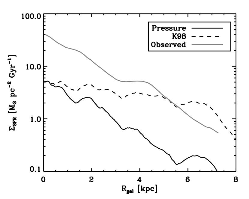
Figure 6.— Star formation rate as a function of galactocentric radius ($R_{gal}$) for NGC 598 (M33). The figure compares the results for the pressure-based star formation prescription in the present work (solid) to that of K98 (dashed) and the measured values (gray, Heyer et al., 2004). The pressure formulation predicts the shape of the observed curve, though the results are offset by a constant factor of 7, implying the star formation efficiency of molecular gas in M33 is dramatically higher than in comparable systems.

Molecule-Rich Galaxies – Finally, we examine the predictions of the pressure-based star formation prescription in the molecule-rich galaxies of Wong & Blitz (2002). In these galaxies, the measured ${\Sigma_{\mathrm{H2}}(\mathrm{CO})}$ is everywhere greater than ${\Sigma_{\mathrm{HI}}}$, so we use Equation 25 to determine the SFR. We compare the K98 prescription and pressure-based results for six galaxies in Figure 7. We omit M101 (NGC 5457) from our analysis because of the narrow range of $R_{gal}$ over which all relevant quantities are measured. The observed star formation data are those of Wong & Blitz (2002) for the case where $A_{V}\propto N(\mbox{H})$. For these galaxies, the pressure-based star formation prediction agrees well with that of K98 since the galaxies are predominantly molecular. The two predictions agree reasonably well with observed data except for NGC 4321. The Wong & Blitz (2002) observations are insufficiently sensitive to go into the low pressure regime where the pressure-based formulation may do better at reproducing the observed results. Indeed, it is when $R_{mol}\lesssim 2$ that the relations diverge, which will occur for the outer regions of large spirals, H I-rich dwarfs such as dwarf irregulars, and damped Ly-$\alpha$ systems. For these objects, our predicted star formation rates are significantly lower than those of Kennicutt (1998). Since dwarf irregulars often show episodic star formation, our prescription assumes that enough dIrrs are observed to be representative of the population as a whole.

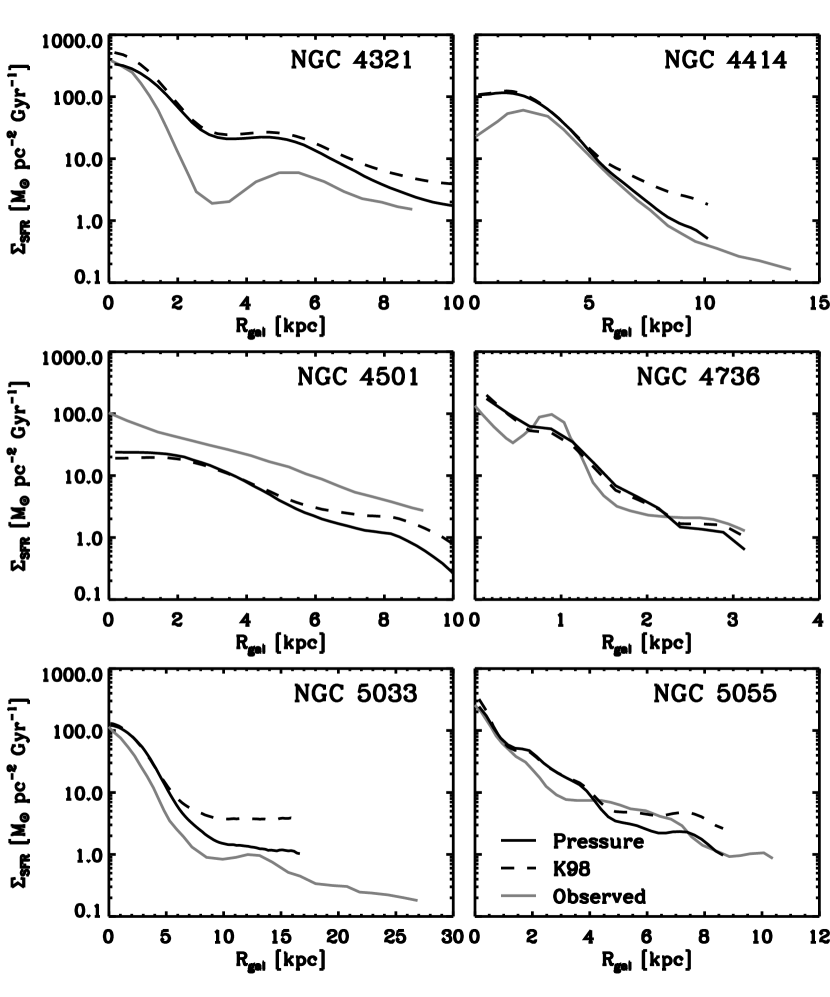
Figure 7.— Star formation rate as a function of galactocentric radius ($R_{gal}$) for six molecule-rich galaxies studied in Wong & Blitz (2002). For each panel, the observed star formation rate is shown as a gray curve, the pressure-based prediction as a solid curve and the K98 prediction as a dashed curve. All three curves agree reasonably well, but the pressure prediction tends to reproduce results in the outer regions of the galaxies well.

We also compare the observed global star formation rates in these Table 3. The global star formation rates given in the table are determined by integrating under each of the curves. On the basis of the data in this table, there is no significant difference in using K98 or our Equation 25 to predict star formation rates for these large, molecule-rich galaxies, though the pressure-based prescription tends to give somewhat higher values. A difference of about 15% is expected as a result of a somewhat higher value of the coefficient in Equation 17 compared to the K98 value.

Table 3Results

Galaxy	$M_{\mathrm{H2}}$	$\dot{M}_{\star}$, Observed	$\dot{M}_{\star}$, Pressure	$\dot{M}_{\star}$, K98
	($10^{9}~{}M_{\odot}$)	($M_{\odot}~{}\mbox{yr}^{-1}$)	($M_{\odot}~{}\mbox{yr}^{-1}$)	($M_{\odot}~{}\mbox{yr}^{-1}$)
NGC 4321	6.5	1.8	10.4	6.6
NGC 4414	4.4	3.0	6.2	4.9
NGC 4501	1.6	3.2	1.4	1.2
NGC 4736	0.3	0.3	0.2	0.4
NGC 5033	4.2	1.9	5.2	3.8
NGC 5055	1.6	1.2	1.5	1.7

galaxies

4.2.4 Comparison with Simulations

A fundamental difference between the two relations comes when one wishes to compare the predictions of the star formation rate from numerical simulations with that of the star formation prescriptions. In the K98 formulations, since the star formation rate depends only on the total amount of gas, the state of the gas is unimportant. Here, we argue that the state of the gas is of central importance, and can be determined by Equation 13 from the total amount of gas and knowledge of the gas pressure. Thus, high column density, low-pressure gas should have relatively few molecules and therefore a low star formation rate. High column density, high-pressure gas should have about the same star formation rate in both formulations, because there will be nearly complete conversion of atomic to molecular gas.

5. Summary and Conclusions

• We show that the ratio of atomic to molecular gas in galaxies is determined by hydrostatic pressure and that the relationship between the two is nearly linear, over three orders of magnitude in pressure. The rms deviation of individual points from the mean relation is a 0.26 dex, or 80%. The scatter of the binned data for all of the galaxies is 0.15 dex, only 38%.

• In addition to very similar slopes, the galaxies have only a small range in zero points, except for three galaxies that are interacting with their environments.

• The dispersion of measurements within individual galaxies varies widely from galaxy to galaxy, with some galaxies showing extraordinarily small dispersions.

• Although some of the correlation is driven by the appearance of $\Sigma_{\mathrm{H2}}$ on both axes at values of high $R_{mol}$, measurement of the power law index of the pressure is nevertheless reliable.

• Although the galaxies in our sample are missing S0, E, strong starburst and Seyferts, we probe a large range in mass, metallicity and column density, suggesting that the $P_{ext}-R_{mol}$ relation has wide applicability.

• Even though star formation is associated with dense gas traced by CS and HCN, we show that CO is as good a tracer of star formation in galaxies as HCN, even in starbursts. This is due to the tight, non-linear relationship between ${\Sigma_{\mathrm{SFR}}}$ and ${\Sigma_{\mathrm{H2}}(\mathrm{CO})}$ in galaxies.

• We derive a pressure-based prescription for star formation in galaxies that is based on the $P-R_{mol}$ relation derived in this paper. It differs from K98 for the outer regions of large spirals, dwarf galaxies, damped Lyman alpha systems and other molecule-poor galaxies. For molecule-rich galaxies, the prescription has a form similar to that of K98.

References

- Bell & de Jong (2001) Bell, E. F. & de Jong, R. S. 2001, ApJ, 550, 212
- Blitz (1993) Blitz, L. 1993, in Protostars and Planets III, 125–161
- Blitz et al. (2006) Blitz, L., Fukui, Y., Kawamura, A., Leroy, A., Mizuno, N., & Rosolowsky, E. 2006, in Protostars and Planets V, 1–18
- Blitz & Rosolowsky (2004) Blitz, L. & Rosolowsky, E. 2004, ApJ, 612, L29
- Braun (1995) Braun, R. 1995, A&AS, 114, 409
- Burton (1971) Burton, W. B. 1971, A&A, 10, 76
- Cayatte et al. (1994) Cayatte, V., Kotanyi, C., Balkowski, C., & van Gorkom, J. H. 1994, AJ, 107, 1003
- Cayatte et al. (1990) Cayatte, V., van Gorkom, J. H., Balkowski, C., & Kotanyi, C. 1990, AJ, 100, 604
- Condon (1992) Condon, J. J. 1992, ARA&A, 30, 575
- Dame (1993) Dame, T. M. 1993, in AIP Conf. Proc. 278: Back to the Galaxy, 267–278
- de Vaucouleurs et al. (1991) de Vaucouleurs, G., de Vaucouleurs, A., Corwin, H. G., Buta, R. J., Paturel, G., & Fouque, P. 1991, Third Reference Catalogue of Bright Galaxies (Volume 1-3, XII, 2069 pp. 7 figs.. Springer-Verlag Berlin Heidelberg New York)
- Dehnen & Binney (1998) Dehnen, W. & Binney, J. 1998, MNRAS, 294, 429
- Deul & van der Hulst (1987) Deul, E. R. & van der Hulst, J. M. 1987, A&AS, 67, 509
- Dickey et al. (1990) Dickey, J. M., Hanson, M. M., & Helou, G. 1990, ApJ, 352, 522
- Elmegreen (1993) Elmegreen, B. G. 1993, ApJ, 411, 170
- Engargiola et al. (2003) Engargiola, G., Plambeck, R. L., Rosolowsky, E., & Blitz, L. 2003, ApJS, 149, 343
- Gao & Solomon (2004) Gao, Y. & Solomon, P. M. 2004, ApJ, 606, 271
- Garnett (1990) Garnett, D. R. 1990, ApJ, 363, 142
- Giovanelli & Haynes (1983) Giovanelli, R. & Haynes, M. P. 1983, AJ, 88, 881
- Guesten & Mezger (1982) Guesten, R., & Mezger, P. G. 1982, Vistas in Astronomy, 26, 159
- Guibert et al. (1978) Guibert, J., Lequeux, J., & Viallefond, F. 1978, A&A, 68, 1
- Haynes et al. (1979) Haynes, M. P., Giovanelli, R., & Roberts, M. S. 1979, ApJ, 229, 83
- Helfer & Blitz (1997a) Helfer, T. T. & Blitz, L. 1997a, ApJ, 478, 233
- Helfer & Blitz (1997b) —. 1997b, ApJ, 478, 162
- Helfer et al. (2003) Helfer, T. T., Thornley, M. D., Regan, M. W., Wong, T., Sheth, K., Vogel, S. N., Blitz, L., & Bock, D. C.-J. 2003, ApJS, 145, 259
- Henry & Howard (1995) Henry, R. B. C. & Howard, J. W. 1995, ApJ, 438, 170
- Heyer et al. (2004) Heyer, M. H., Corbelli, E., Schneider, S. E., & Young, J. S. 2004, ApJ, 602, 723
- Hippelein et al. (2003) Hippelein, H., Haas, M., Tuffs, R. J., Lemke, D., Stickel, M., Klaas, U., & Völk, H. J. 2003, A&A, 407, 137
- Jarrett et al. (2003) Jarrett, T. H., Chester, T., Cutri, R., Schneider, S. E., & Huchra, J. P. 2003, AJ, 125, 525
- Kenney & Young (1989) Kenney, J. D. P. & Young, J. S. 1989, ApJ, 344, 171
- Kennicutt (1998) Kennicutt, R. C. 1998, ApJ, 498, 541
- Kim et al. (1998) Kim, S., Staveley-Smith, L., Dopita, M. A., Freeman, K. C., Sault, R. J., Kesteven, M. J., & McConnell, D. 1998, ApJ, 503, 674
- Knapen et al. (1993) Knapen, J. H., Cepa, J., Beckman, J. E., Soledad del Rio, M., & Pedlar, A. 1993, ApJ, 416, 563
- Kregel et al. (2002) Kregel, M., van der Kruit, P. C., & de Grijs, R. 2002, MNRAS, 334, 646
- Kroupa (1995) Kroupa, P. 1995, MNRAS, 277, 1522
- Krumholz & McKee (2005) Krumholz, M. R. & McKee, C. F. 2005, ApJ, 630, 250
- Lada (1992) Lada, E. A. 1992, ApJ, 393, L25
- Leroy et al. (2006) Leroy, A., Bolatto, A., Walter, F., & Blitz, L. 2006, ApJ, 0, submitted
- Levine et al. (2006) Levine, E., Blitz, L., & Heiles, C. 2006, ApJ, 000, in press
- Lyne et al. (1985) Lyne, A. G., Manchester, R. N., & Taylor, J. H. 1985, MNRAS, 213, 613
- Malhotra (1995) Malhotra, S. 1995, ApJ, 448, 138
- Martin & Kennicutt (2001) Martin, C. L. & Kennicutt, R. C. 2001, ApJ, 555, 301
- Meier & Turner (2004) Meier, D. S. & Turner, J. L. 2004, AJ, 127, 2069
- Miller & Scalo (1979) Miller, G. E. & Scalo, J. M. 1979, ApJS, 41, 513
- Mooney & Solomon (1988) Mooney, T. J. & Solomon, P. M. 1988, ApJ, 334, L51
- Murgia et al. (2002) Murgia, M., Crapsi, A., Moscadelli, L., & Gregorini, L. 2002, A&A, 385, 412
- Nieten et al. (2006) Nieten, C., Neininger, N., Guélin, M., Berkhuijsen, E., & Beck, R. 2006, A&A, 000, in press
- Olling & Merrifield (2001) Olling, R. P. & Merrifield, M. R. 2001, MNRAS, 326, 164
- Prantzos & Aubert (1995) Prantzos, N., & Aubert, O. 1995, A&A, 302, 69
- Rana (1991) Rana, N. C. 1991, ARA&A, 29, 129
- Regan et al. (2004) Regan, M. W., Thornley, M. D., Bendo, G. J., Draine, B. T., Li, A., Dale, D. A., Engelbracht, C. W., Kennicutt, R. C., Armus, L., Calzetti, D., Gordon, K. D., Helou, G., Hollenbach, D. J., Jarrett, T. H., Kewley, L. J., Leitherer, C., Malhotra, S., Meyer, M., Misselt, K. A., Morrison, J. E., Murphy, E. J., Muzerolle, J., Rieke, G. H., Rieke, M. J., Roussel, H., Smith, J. T., & Walter, F. 2004, ApJS, 154, 204
- Reynolds (1989) Reynolds, R. J. 1989, ApJ, 339, L29
- Rosolowsky & Blitz (2005) Rosolowsky, E. & Blitz, L. 2005, ApJ, 623, 826
- Rots et al. (1990) Rots, A. H., Crane, P. C., Bosma, A., Athanassoula, E., & van der Hulst, J. M. 1990, AJ, 100, 387
- Salpeter (1955) Salpeter, E. E. 1955, ApJ, 121, 161
- Schmidt (1959) Schmidt, M. 1959, ApJ, 129, 243
- Scoville & Good (1989) Scoville, N. Z. & Good, J. C. 1989, ApJ, 339, 149
- Shostak & van der Kruit (1984) Shostak, G. S. & van der Kruit, P. C. 1984, A&A, 132, 20
- Thean et al. (1997) Thean, A. H. C., Mundell, C. G., Pedlar, A., & Nicholson, R. A. 1997, MNRAS, 290, 15
- Thornley & Mundy (1997a) Thornley, M. D. & Mundy, L. G. 1997a, ApJ, 484, 202
- Thornley & Mundy (1997b) —. 1997b, ApJ, 490, 682
- van der Kruit & Shostak (1982) van der Kruit, P. C. & Shostak, G. S. 1982, A&A, 105, 351
- van der Kruit & Shostak (1984) —. 1984, A&A, 134, 258
- van Zee & Bryant (1999) van Zee, L. & Bryant, J. 1999, AJ, 118, 2172
- Wilcots & Miller (1998) Wilcots, E. M. & Miller, B. W. 1998, AJ, 116, 2363
- Wong & Blitz (2002) Wong, T. & Blitz, L. 2002, ApJ, 569, 157
- Wong et al. (2004) Wong, T., Blitz, L., & Bosma, A. 2004, ApJ, 605, 183
- Wu et al. (2005) Wu, J., Evans, N. J., Gao, Y., Solomon, P. M., Shirley, Y. L., & Vanden Bout, P. A. 2005, ArXiv Astrophysics e-prints
- Young et al. (1995) Young, J. S., Xie, S., Tacconi, L., Knezek, P., Viscuso, P., Tacconi-Garman, L., Scoville, N., Schneider, S., Schloerb, F. P., Lord, S., Lesser, A., Kenney, J., Huang, Y., Devereux, N., Claussen, M., Case, J., Carpenter, J., Berry, M., & Allen, L. 1995, ApJS, 98, 219
- Young (2002) Young, L. M. 2002, AJ, 124, 788
- Zhang et al. (1993) Zhang, X., Wright, M., & Alexander, P. 1993, ApJ, 418, 100