Lyman Limit Systems in Cosmological Simulations

Abstract

We used cosmological simulation with self-consistent radiative transfer to investigate the physical nature of Lyman limit systems at $z=4$. In agreement with previous studies, we find that most of Lyman-limit systems are ionized by the cosmological background, while higher column density systems seem to be illuminated by the local sources of radiation. In addition, we find that most of Lyman limit systems in our simulations are located within the virial radii of galaxies with a wide range of masses, and are physically associated with them (“bits and pieces” of galaxy formation). While the finite resolution of our simulations cannot exclude an existence of a second population of self-shielded, neutral gas clouds located in low mass dark matter halos (“minihalos”), our simulations are not consistent with “minihalos” dominating the total abundance of Lyman limit systems.

1 Introduction

The hydrogen absorption system observed in spectra of distant quasars are traditionally subdivided into Lyman-$\alpha$ forest ($N_{{\rm HI}}\lesssim 1.6\times 10^{17}\mbox{\,cm}^{2}$), Lyman-limit systems ($1.6\times 10^{17}\mbox{\,cm}^{2}\lesssim N_{{\rm HI}}\lesssim 10^{20}\mbox{\,cm}^{2}$), and damped Lyman-$\alpha$ systems ($N_{{\rm HI}}\gtrsim 10^{20}\mbox{\,cm}^{2}$). Amazingly, among these three classes, the Lyman-limit systems are least understood, both observationally and theoretically. This is quite unfortunate, given that the Lyman-limit systems dominate the absorption of ionizing photons in the universe (Miralda-Escudé, 2003), and are, therefore, crucial for understanding the transfer of ionizing radiation in the IGM and the interactions between the early galaxies and quasars and their environments.

Previous attempts to model Lyman-limit systems in cosmological simulations identified them with low mass dark matter halos, filled with neutral, self-shielded gas (Katz et al., 1996; Gardner et al., 1997, 2001). On the other hand, the observations of neutral hydrogen in the vicinity of the Milky Way galaxy uncovered a large population of High Velocity Clouds (HVCs) that could plausible be low redshift counterparts of Lyman-limit systems (Oort, 1966; Verschuur, 1969; Blitz et al., 1999; Maloney & Putman, 2003; Putman et al., 2003).

In this paper we use cosmological simulations with the self-consistent treatment of the transfer of ionizing radiation to address the question of the nature of Lyman-limit systems, as their appear in the simulations. Another advantage of the simulations we use here is that they are designed to model the reionization of the universe, and so achieve a reasonable agreement with the SDSS observational data on the Lyman-$\alpha$ forest at $z>5$ (Fan et al., 2006; Gnedin & Fan, 2006).

2 Simulations

Simulations used in this paper have been run with the “Softened Lagrangian Hydrodynamics” (SLH) code (Gnedin, 2000, 2004). Simulations include dark matter, gas, star formation, chemistry, and ionization balance in the primordial plasma, and three-dimensional radiative transfer. The simulations described in this paper use a flat $\Lambda$CDM cosmology with values of cosmological parameters as determined by the first year WMAP data (Spergel et al., 2003).

We use two sets of simulations in this paper. The two sets differ by the size of the computational box: in the first set the computational box has the size of $4h^{-1}$ comoving Mpc, while in the second set the box is $8h^{-1}$ comoving Mpc on a side.

The primary simulations in each of two sets are runs L4N128 and L8N128 from Gnedin & Fan (2006). Both of them include $128^{3}$ dark matter particles and the same number of quasi-Lagrangian mesh cells for the gas evolution, as well as a smaller number of stellar particles that formed continuously during the simulation.

As Gnedin & Fan (2006) emphasized, these simulations provide an adequate fit to the evolution of the mean transmitted flux in the Lyman-$\alpha$ forest between $5<z<6.2$, but overproduce the opacity in the forest at $z<5$. As we show below, they also overproduce Lyman-limit systems.

The simulations, however, contain adjustable parameters; the one of importance here is the ionizing efficiency parameter $\epsilon_{UV}$, that controls the amount of ionizing radiation emitted per unit mass of stars formed in the simulation. This parameter depends on the numerical resolution of the simulation and on the details of stellar feedback and radiative transfer implementations, and has no clear physical interpretation. It can be thought of as a fraction of ionizing radiation escaping from the spatial scales unresolved in the simulation (it has no direct relation to the widely used “escape fraction” quantity).

Since we treat the ionizing efficiency as a free parameter, we can adjust it to obtain a better agreement with the observational data. For that purpose, we run additional simulations in which we increased the ionizing efficiency by an additional factor $q$. Because in this paper we only concentrate on comparing the simulations with the data at $z=4$, and in order to save computational resources, we only rerun the simulations with different values of the ionizing intensity from $z=4.3$ to $z=4$. The redshift interval of $\Delta z=0.3$ corresponds to the time interval of $130\mbox{\,Myr}$, which is some 4,000 larger than the mean photoionization time at this redshift (McDonald et al., 2002), and, thus, should be more than sufficient for establishing a new photoionization equilibrium even in the lowest density regions. To be on the safe side, we also rerun one of the simulations from $z=4.6$ to $z=4$, and the results for the Lyman-$\alpha$ mean transmitted flux and the column density distribution of the Lyman-limit systems from that simulation are indistinguishable from the analogous run started at $z=4.3$.

In order to make references to specific simulations transparent, we label each simulation with a letter L followed by the value of the linear size of the computational volume (measured in $h^{-1}\mbox{\,Mpc}$), followed by the letter “q” and the value of the ionization enhancement parameter $q$. For example, the primary simulations in each set are thus labeled L4q1 and L8q1, while a $4h^{-1}\mbox{\,Mpc}$ simulation with 6 times higher ionizing efficiency is labeled L4q6. In the $4h^{-1}\mbox{\,Mpc}$ set we run simulations L4q1, L4q2, L4q6, and L4q10, while in the $8h^{-1}\mbox{\,Mpc}$ set we run L8q1 and L8q6.

The Lyman Limit systems are found by casting $10000$ lines of sight through the simulation box, allowing us to sample the simulation box finely enough to find even rare absorbers. The lines of sight are cast in random directions and cover a redshift range of $\delta z=0.033$ for the $8h^{-1}\mbox{\,Mpc}$ boxes. This narrow extent in redshift space makes it difficult to search for the Lyman-limit edge in the spectra. Thus, to find the regions of high optical depth along the lines of sight, we search for peaks in $\lambda d\tau_{LL}/{d\lambda}$.

This is similar to searching for an absorption line. For example, a Lyman-$\alpha$ absorption line profile can be described with (we ignore natural width of the line here):

$$\tau_{\alpha}=\frac{\tau_{0}}{b\sqrt{\pi}}\int d\lambda^{\prime}e^{-\frac{(\lambda-\lambda^{\prime})^{2}}{b^{2}}}\delta(\lambda^{\prime}-\lambda).$$ (1)

When considering $\lambda d\tau_{LL}/d\lambda$ instead of $\tau_{LL}$, the Lyman limit edge becomes the delta-function in frequency, in full analogy with the absorption line profile. Thus, a Lyman-limit system appears as a peak in the quantity

$$\tilde{\tau}_{LL}=\frac{1}{b\sqrt{\pi}}\int d\lambda^{\prime}e^{-\frac{(\lambda-\lambda^{\prime})^{2}}{b^{2}}}\lambda^{\prime}\frac{d\tau_{LL}}{d\lambda^{\prime}}.$$ (2)

This substitution allows us to use software tools, already developed for finding absorption lines in synthetic spectra, for finding Lyman-limit systems in the simulated synthetic spectra. In particular, the value of $\tilde{\tau}_{LL}$ at the “line” center is directly proportional to the neutral hydrogen column density, $\tilde{\tau}_{LL}=\sigma_{LL}N_{HI}$, where $\sigma_{LL}=6.3\times 10^{-18}\rm{cm^{2}}$ is the hydrogen photoionization cross-section. All regions in the spectra where $\tilde{\tau}_{LL}\geq 1.0$, corresponding to column densities of $N_{HI}>1.6\times 10^{17}\rm{cm^{-2}}$, are selected as Lyman-limit systems.

After casting the lines of sight, the positions of these regions (in 3D space) and their opacities are determined. We also compute other characteristics such as local photoionization rate, column density and neutral fraction of the gas. This information allows us to investigate whether the systems are ionized by local sources or by the cosmological background radiation.

Finding the positions of the Lyman-limit systems in the simulation box and determining the position of the galaxies in the simulation allows us to determine whether each Lyman Limit system can be associated with a galaxy.

Galaxies in the simulation are identified with gravitationally bound objects, found with the DENMAX algorithm (Bertschinger & Gelb, 1991). The DENMAX algorithm works by constructing the finite resolution smooth total (dark matter + gas + stars) density field from the simulation data. It then identifies density maxima and associates them with bound objects. This approach has a major advantage for our purposes here, since it allows us to assign a specific meaning to the word “associated”. Since each galaxy is represented by DENMAX as a density hill, we will call all points in space that lie on that hill as “associated” with that galaxy. In other words, a point of space is “associated” with a given galaxy if, by moving against the density gradient from that point one would eventually end up at the center of the galaxy.

DENMAX separates all points of space into four distinct categories:

• points gravitationally bound to a given galaxy;

• points associated with a given galaxy but not gravitationally bound to it (i.e. points lying on the galaxy density hill, but outside the virial radius);

• unassociated points (i.e. points not associated with any galaxy, like points in the middle of the void); and

• points associated with unresolved galaxies (i.e. points belonging to the density hill too small to be qualified as a resolved galaxy).

We use this classification below to describe locations of Lyman-limit systems in space.

3 Results

The main goal of this work is to investigate the physical properties of the Lyman limit systems themselves, such as neutral fraction and photoionization rate, but also what kind of galaxies they are associated with.

To begin, we have to normalize the amount of photons in the simulation box to the observations, so that the population of simulated Lyman-limit systems corresponds to the systems that are observed. This is done using the number density of Lyman limit systems per column density and adjusting the ionization efficiency to reduce the amount of Lyman-limit systems produced. Another observational parameter that can be used to fit the simulations to observations is the mean transmitted flux in Lyman-$\alpha$.

Figure 1: Shown are the number densities of Lyman-Limit systems for three different runs, each with $4h^{-1}\mbox{\,Mpc}$ box size. The fits are overlaid. Top: L4q1, middle: L4q6, bottom: L4q10.

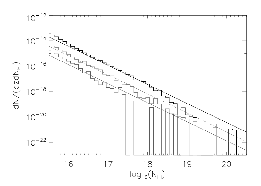
Figure 1 shows the number density of the Lyman limit systems versus their column density for 3 different runs with varying ionization efficiency $q$. The top run, with its fitted line overlaid, corresponds to L4q1, which is the the run with the default value of the ionization efficiency. The middle run is L4q6, where the ionization efficiency is increased by a factor of 6 and the bottom run is run L4q10, with a ionization efficiency $q=10$. The overlaid fits are best-fit power laws with the slope $-1.5$ (Petitjean et al., 1993; Miralda-Escudé, 2003).

For the L4q6 run the fitted line exactly corresponds to the observed number density obtained by Storrie-Lombardi et al. (1994). The other two fits have the same power law, but different amplitudes. L4q1 had a number density of Lyman-limit systems too high to fit the observations. This illustrates that the original simulations, while fitting the mean transmitted flux in the Lyman-$\alpha$ forest at $z>5$, significantly overpredict the amount of Lyman-limit systems at $z=4$.

Figure 2: Similarly to Figure 1, this graph shows the number density distribution of Lyman limit systems for two $8h^{-1}\mbox{\,Mpc}$ runs (in black, L8q1 on top and L8q6 on bottom) and $4h^{-1}\mbox{\,Mpc}$ run L4q6 (in grey). Their power law fits are included.

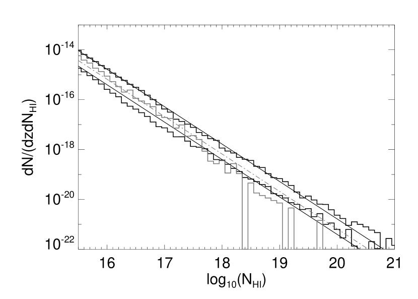
Figure 2 similarly shows the number density distribution with column density for the two $8h^{-1}\mbox{\,Mpc}$ runs L8q1 and L8q6 and for comparison the $4h^{-1}\mbox{\,Mpc}$ run L4q6. The highest distribution is again L8q1 with the lowest ionizing efficiency. The other $8h^{-1}\mbox{\,Mpc}$ run also has the same $q=6$. There is good agreement between the $4$ and the $8h^{-1}\mbox{\,MpC}$ run at $N_{HI}>10^{17}\mbox{\,cm}^{2}$. At lower column densities the larger box size lacks enough resolution to fully resolve the Lyman-$\alpha$ forest. Thus the number of Lyman-$\alpha$ forest systems is too low at lower column densities, which can be seen from the disagreement for the two $q=6$ distributions.

Figure 3: This graph shows the ionization efficiency $q$ that was used as a fitting parameter for the simulations on the x-axis and shown on the y-axis are the two observational constraints: amplitude of the number density fit, A, and the mean transmitted flux $F_{mean}$.

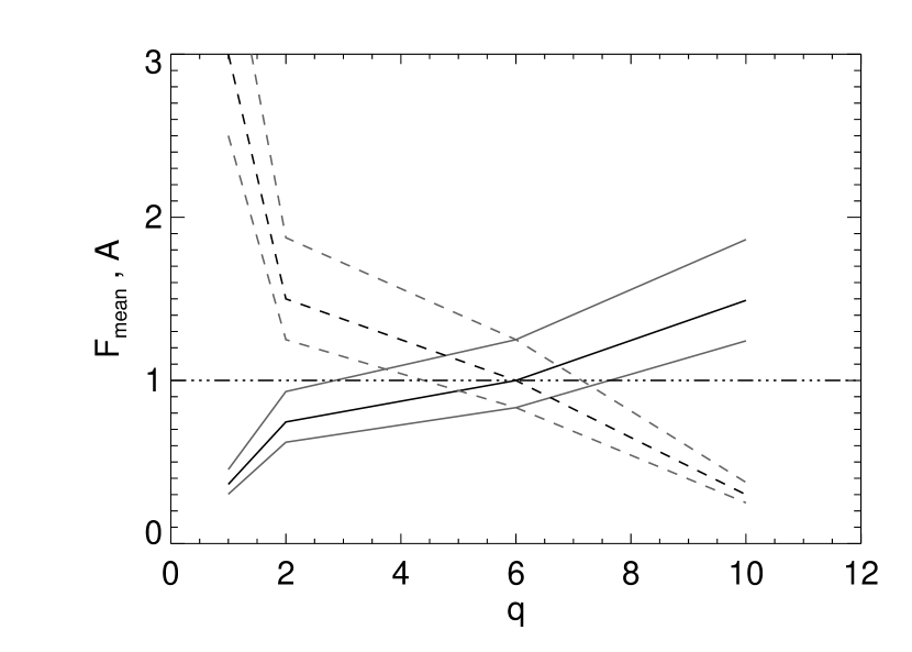
In Figure 3 the dependence on the parameter $q$ is illustrated. The solid lines show the mean transmitted flux in the Lyman-$\alpha$ forest normalized by the observational values of $0.55$ at $z=4$. For higher $q$ there is more flux transmitted as the increased ionizing intensity ionizes more of the initially neutral gas. The dashed lines show the amplitude of the power law that is needed to fit the number density of Lyman-limit systems as described above in Figures 1 and  2. Here, for lower ionization efficiency the offset is lower, for $q=6$ the offset is unity, since the number density distribution is best fit by the observational value. The horizontal line shows the observational values for both parameters since we normalize by the observed value. The gray lines correspond to a $20\%$ error, as is expected from the observations. This plot illustrates that we can fit two different observables with just one parameter, the ionization efficiency, and that increasing this parameter by a factor of $6$ from the values used in Gnedin & Fan (2006) fits the observations at $z=4$.

Figure 4: Distribution of Lyman limit system optical depth versus the neutral fraction of gas.

Figure 4 shows the distribution of optical depth of the Lyman-limit systems versus hydrogen neutral fraction. There is a tight relation of the optical depth with neutral fraction, the higher $\tilde{\tau}_{LL}$, the less ionized the system. The remarkable conclusion from this is that the systems are substantially ionized and are not neutral. This implies that the Lyman-limit systems detected in this simulation are not small self-shielded clumps of neutral gas, but rather diffuse highly non-spherical clouds of gas that happen to be oriented in their longest direction toward an observer.

Figure 5: Similar to Figure 4, this graph shows the distribution of optical depth versus the normalized photoionization rate.

In Figure 5 it is similarly shown how the optical depth depends on the photoionization rate for each Lyman-limit system. These two variables are not as tightly correlated as the optical depth and the neutral fraction. For lower $\tilde{\tau}_{LL}$ systems the normalized photoionization rate $\Gamma/\langle\bar{\Gamma}\rangle$, where $\bar{\Gamma}$ is the average $\Gamma$, is about unity. This means that these systems are ionized by the cosmological background and not by local sources. Systems with higher $\tilde{\tau}_{LL}$ appear to be ionized by local sources because their normalized photoionization rate is higher. This result is in agreement with previous findings by Miralda-Escudé (2005)and Schaye (2006).

One of the questions we investigate is whether the Lyman-limit systems are associated with high or low mass galaxies. At first, we have tried to use a method similar to one used by observational studies of the environment of the Lyman-limit systems at low redshifts (Penton et al., 2002). In observations, the Lyman-limit systems are often associated with a galaxy by finding the nearest object, either along a line of sight or near it. A similar method was also used to analyze the simulations in Katz et al. (1996). There, a relation between the distance to the nearest galaxy and $N_{\rm{HI}}$ of the Lyman-limit systems was shown, and it was concluded that the column density correlates inversely with projected distance, and that Lyman-limit systems either lie in the outer parts of massive protogalaxies or closer to the center of less massive galaxies.

In our case we found that associating the Lyman-limit systems with the nearest object is not necessarily the best option, because such association is strongly dependent on the galaxy sample. When we decrease the mass limit of the sample, thus including less and less massive galaxies in the sample, we find progressively lower mass galaxies closer and closer to a typical Lyman-limit system. This, of course, does not imply that the Lyman-limit systems are physically associated with these low mass galaxies, because low mass galaxies are more numerous, and the distances between even a random subset of points in space to galaxies of progressively smaller masses will be progressively smaller.

Thus, associating the Lyman-limit systems with nearest galaxies could lead to the conclusion that most of the Lyman-limit systems are located in small galaxies. However, using the physical association as permitted by the DENMAX algorithm (§2) - i.e. associating a Lyman-limit system with the galaxy whose “density hill” (i.e. dark matter halo) the Lyman-limit is located on - we find a different result: the Lyman-limit systems are associated with galaxies in a wide range of masses and the small galaxies near them are often physically unrelated satellites of the larger galaxy.

Figure 6: Distribution of optical depths $\tilde{\tau}_{LL}$ of the Lyman-limit systems versus the mass of their associated galaxy.

Figure 6 shows the masses of the galaxies that the Lyman-limit systems are associated with versus the systems’ optical depth. There is no strong dependence on galaxy mass for the optical depth, meaning that the size of the galaxy does not appear to strongly influence the opacity of the Lyman-limit system.

Figure 7: Top Panel: Number of galaxies per mass bin. Bottom Panel: Distribution of distances of the Lyman-limit systems from their associated galaxy with respect to the mass of that galaxy.

The bottom panel of Figure 7 is a graph of the distance of the Lyman-limit system to its associated galaxy and the mass of that galaxy. Overlaid on this correlation is the distance that corresponds to the virial radius for each galaxy mass. The resolution limit of our simulation is about $0.001\mbox{\,Mpc}$, so that we resolve all the distances to the galaxies. The top panel shows the number of galaxies per mass bin for the same mass range as the bottom panel. It is clear from this histogram that there are many more small galaxies that have no Lyman-limit associated with them.

Combining the information from this graph, we find that most of the Lyman-limit systems are within the virial radius of a galaxy, often a relatively massive one. This means that they are either in orbit around or infalling into a galaxy, and not isolated clumps of neutral gas. Using the DENMAX classification of points in space discussed in §2, we find no Lyman-limit systems that are unassociated or associated with unresolved galaxies.

Figure 8: Number of Lyman-limit systems per associated galaxy. Overlaid is the fit corresponding to an equal amount of Lyman-limit systems per unit log in galaxy mass.

Figure 8 extends the discussion from the previous graph by showing the number of Lyman-limit systems associated with galaxies of different masses. There are many more systems per galaxy in the high galaxy mass range around $M_{gal}\sim 10^{10}$ to $M_{gal}\sim 10^{11}$ than for lower masses. Since $dN_{gal}/d\log(M)\sim M^{-1}$, the number of galaxies sharply increases at low masses. In Figure 8 the overlaid power law ($\propto M^{1}$) shows the equal number of Lyman-limit systems per logarithmic bin in mass of galaxies they are associated with. The figure shows that only a small fraction of all Lyman-limit systems are associated with galaxies of $M_{gal}<10^{10}M_{\sun}$. However, this effect might also be related to resolution effects, meaning that the Lyman-limit systems are associated with galaxies of all mass ranges equally.

4 Conclusions

We show that the column density distribution of Lyman-limit systems at $z=4$ in the cosmological simulations that agree with the SDSS measurements of the Lyman-$\alpha$ absorption at $z>5$ in the spectra of high redshift quasars has the same shape as the observed distribution. The abundance of the Lyman-limit system is not necessarily in agreement with the data, but we manage to achieve the agreement with both the observed column density distribution of the Lyman-limit systems and with the mean transmitted flux in the Lyman-$\alpha$ forest by adjusting a single parameter - ionizing efficiency - at $z<5$.

We find that, in the simulation that agrees with the observational data, the lowest column density Lyman-limit systems are mainly illuminated by the cosmological background, in agreement with previous findings of Miralda-Escudé (2005) and Schaye (2006).

However, we also find that all Lyman-limit systems that are resolved in our simulations ($N_{{\rm HI}}\lesssim 10^{20}\mbox{\,cm}^{2}$) are highly ionized and are physically associated with (are in orbit around or falling into) the gravitational well of a large range of galaxy masses ($M_{tot}>10^{10}M_{\sun}$). In other words, they appear as residual “bits and pieces” of the galaxy formation process rather than self-shielded, highly neutral dark matter “minihalos” ($M_{tot}<10^{9}M_{\sun}$).

Because of the finite spatial and mass resolution of our simulations, we can not exclude an existence of the second population of Lyman-limit systems composed of “minihalos”. However, the fact that we are able to fit both the Lyman-limit column density distribution and the mean transmitted flux in the Lyman-$\alpha$ forest at $z=4$ with one adjustable parameter may indicate that the population of Lyman-limit systems arising in “minihalos” is not the dominant one. Other studies have also shown that we can reproduce the observed Lyman-$\alpha$ forest, so that the hidden population cannot have any influence on the Lyman-$\alpha$ forest. Cross-correlating Lyman-limit systems and galaxies could also help determine whether this population is related to “minihalos”.

References

- Bertschinger & Gelb (1991) Bertschinger, E. & Gelb, J. M. 1991, Computers in Physics, 5, 164
- Blitz et al. (1999) Blitz, L., Spergel, D. N., Teuben, P. J., Hartmann, D., & Burton, W. B. 1999, ApJ, 514, 818
- Fan et al. (2006) Fan, X., Strauss, M. A., Becker, R. H., White, R. L., Gunn, J. E., Knapp, G. R., Richards, G. T., Schneider, D. P., Brinkmann, J., & Fukugita, M. 2006, AJ, in press
- Gardner et al. (1997) Gardner, J. P., Katz, N., Hernquist, L., & Weinberg, D. H. 1997, ApJ, 484, 31
- Gardner et al. (2001) —. 2001, ApJ, 559, 131
- Gnedin (2000) Gnedin, N. Y. 2000, ApJ, 535, 530
- Gnedin (2004) —. 2004, ApJ, 610, 9
- Gnedin & Fan (2006) Gnedin, N. Y. & Fan, X. 2006, astroph/0603794
- Katz et al. (1996) Katz, N., Weinberg, D. H., Hernquist, L., & Miralda-Escude, J. 1996, ApJ, 457, L57+
- Maloney & Putman (2003) Maloney, P. R. & Putman, M. E. 2003, ApJ, 589, 270
- McDonald et al. (2002) McDonald, P., Miralda-Escudé, J., & Cen, R. 2002, ApJ, 580, 42
- Miralda-Escudé (2003) Miralda-Escudé, J. 2003, ApJ, 597, 66
- Miralda-Escudé (2005) —. 2005, ApJ, 620, L91
- Oort (1966) Oort, J. H. 1966, Bull. Astr. Inst. Netherlands, 18, 421
- Penton et al. (2002) Penton, S. V., Stocke, J. T., & Shull, J. M. 2002, ApJ, 565, 720
- Petitjean et al. (1993) Petitjean, P., Webb, J. K., Rauch, M., Carswell, R. F., & Lanzetta, K. 1993, MNRAS, 262, 499
- Putman et al. (2003) Putman, M. E., Bland-Hawthorn, J., Veilleux, S., Gibson, B. K., Freeman, K. C., & Maloney, P. R. 2003, ApJ, 597, 948
- Schaye (2006) Schaye, J. 2006, astroph/0409137
- Spergel et al. (2003) Spergel, D. N., Verde, L., Peiris, H., & et al. 2003, ApJS, 148, 175
- Storrie-Lombardi et al. (1994) Storrie-Lombardi, L. J., McMahon, R. G., Irwin, M. J., & Hazard, C. 1994, ApJ, 427, L13
- Verschuur (1969) Verschuur, G. L. 1969, ApJ, 156, 771