Model selection forecasts for the spectral index from the Planck satellite

Abstract

The recent WMAP3 results have placed measurements of the spectral index $n_{{\rm S}}$ in an interesting position. While parameter estimation techniques indicate that the Harrison–Zel’dovich spectrum $n_{{\rm S}}=1$ is strongly excluded (in the absence of tensor perturbations), Bayesian model selection techniques reveal that the case against $n_{{\rm S}}=1$ is not yet conclusive. In this paper, we forecast the ability of the Planck satellite mission to use Bayesian model selection to convincingly exclude (or favour) the Harrison–Zel’dovich model.

I Introduction

One of the key goals of cosmology is to probe the nature of the primordial perturbations, for instance to seek support for the inflationary cosmology. The simplest models of inflation predict adiabatic gaussian density perturbations of approximately power-law form, characterized by the spectral index $n_{{\rm S}}$, and in addition a spectrum of gravitational wave perturbations (see Ref. LL for an overview).

The ability of experiments, actual or proposed, to explore such questions is typically framed in terms of parameter estimation, for instance by forecasting the expected uncertainty on $n_{{\rm S}}$ given a particular assumed fiducial model. However, it has been stressed in a number of papers recently L04 ; T ; MPL ; MPCLK that many of the key questions are not ones of parameter estimation, but of model selection Jeff ; MacKay ; Gregory . Model selection problems are characterized by an uncertainty in the choice of parameters to vary in a fit to data, rather than of the values of a parameter set chosen by hand. The discovery of any new physical effect in data is indicated by the need to include new parameters, possible examples being non-zero spatial curvature, time variation of the dark energy density, or the existence of tensor perturbations. Early cosmological applications of this technique were given in Ref. ev .

Since many of the most important questions are ones of model selection rather than parameter estimation, it follows that the capabilities of experiments should also be quantified by model selection criteria rather than parameter uncertainty forecasts alone. This is the viewpoint adopted in recent papers by Trotta T , whose Expected Posterior Odds (ExPO) forecasting technique estimates the probability of new data requiring new parameters, and by Mukherjee et al. MPCLK who use Bayes factor plots to compare the ability of different experiments to decisively select between models.

Mukherjee et al. MPCLK illustrated model selection forecasting using dark energy surveys, looking at a two-parameter dark energy model versus a cosmological constant model. The same general approach is applicable in many other contexts. In this paper, we carry out model selection forecasting for the Planck satellite cosmic microwave background project, focussing on its ability to measure the spectral index $n_{{\rm S}}$. This is particularly timely as the recent release of the three-year WMAP data wmap3 has placed this parameter in the zone around three-sigma where the application of model selection techniques is at its most crucial T . In a companion paper to this one, Parkinson et al. PML have shown that the case for $n_{{\rm S}}\neq 1$ is far from decisive at present.

We assume throughout that there are no tensor perturbations. While it would be interesting to explore models including tensors, thus properly probing the inflationary space, at present doing $n_{{\rm S}}$ alone stretches our supercomputer resources to their limit. In this regard model selection forecasting is much more challenging than analysis of real data, as instead of having a single dataset to analyze, one has to create and analyze simulated datasets for a range of possible models and model parameters.

II Model selection forecasts for $n_{{\rm S}}$

II.1 Model selection forecasting

The philosophical underpinning of model selection forecasting was described in Mukherjee et al. MPCLK and we summarize it only very briefly here. Given a particular dataset, simulated or real, model selection is carried out by evaluation of a model selection statistic for each model, where the term model refers to a choice of parameters to be varied plus a set of prior ranges for those parameters. The usual statistic of choice is the Bayesian evidence $E$, also known as the marginalized likelihood. The ratio of evidences between two models is known as the Bayes factor, $B_{10}=E(M_{1})/E(M_{0})$, where $M_{1}$ and $M_{0}$ indicate the two models under consideration. By plotting the Bayes factor using datasets generated as a function of a parameter of interest, one uncovers the regions of parameter space in which a given experiment would be able to decisively select between the two models, and also those regions where the comparison would be inconclusive.

In short, the advantages of model selection over parameter estimation forecasting are as follows MPCLK .

• Experiments motivated by model selection questions should be quantified by their ability to answer such questions.

• Data is simulated at each point in the parameter space, rather than at only one or more fiducial models. Indeed in parameter estimation plots people commonly simulate data for the model that they hope to rule out, rather than for the true model that would allow that exclusion.

• Model selection analyses can attribute positive support for a simpler model, rather than only showing consistency.

• Gaussian approximations to the likelihood are not made, such as in parameter estimation forecasting done using Fisher matrices.

In assessing the significance of a model comparison, a useful guide is given by the Jeffreys’ scale Jeff . Labelling as $M_{1}$ the model with the higher evidence, it rates $\ln B_{10}<1$ as ‘not worth more than a bare mention’, $1<\ln B_{10}<2.5$ as ‘substantial’, $2.5<\ln B_{10}<5$ ‘strong’ to ‘very strong’ and $5<\ln B_{10}$ as ‘decisive’. Note that $\ln B_{10}=5$ corresponds to odds of 1 in about 150, and $\ln B_{10}=2.5$ to odds of 1 in 13.

A model selection analysis of the Planck satellite’s capabilities to constrain $n_{{\rm S}}$ was previously given by Trotta T using his ExPO technique. This seeks to estimate the probability, based on current knowledge of parameters, of the Planck mission being able to carry out a decisive model comparison. Our aim is rather different; we seek to delineate the parameter values the Universe would have to have in order for a decisive model comparison to be made. However we will end by additionally making an ExPO-style forecast, though with a somewhat different implementation to Trotta’s.

Another related paper is Bridges et al. BLH , who simulate data for a model with constant $n_{{\rm S}}$ and compare the evidences for a set of initial power spectrum models. They do not however explore different values of the spectral index.

It may seem strange that model selection approaches can give results in apparent conflict with parameter estimation. However, this is a well-known phenomenon called Lindley’s paradox L ; T ; the idea that there is a universal significance level such as 95% beyond which things become interesting is inconsistent with Bayesian reasoning, which shows that such a threshold should depend both on the data properties and the prior parameter ranges. The Lindley paradox usually manifests itself for results with significance in the range two to four sigma T , which as it happens is exactly where WMAP3 has placed $n_{{\rm S}}$.

II.2 Simulating Planck data

In order to give a good estimate of Planck’s abilities, we need accurate data simulations. Simulated Planck data was generated by Bridges et al. BLH for their model selection analysis, but they simply assumed cosmic variance limited temperature anisotropies out to $\ell=2000$. We adopt a rather more sophisticated approach, as follows.

We simulate the temperature and polarization (TT, TE, and EE) spectra. We choose not to include $B$-polarization for simplicity; as we do not include tensors there are no primordial $B$ modes, and the shorter-scale $B$-modes generated by gravitational lensing will not supply significant constraining power on the specific models we are considering.

We use three temperature channels, of specifications similar to the HFI channels of frequency 100 GHz, 143 GHz, and 217 GHz. Following the current Planck documentation, the intensity sensitivities of these channels are taken as 6.8 $\mu$K, 6.0 $\mu$K, and 13.1 $\mu$K respectively, corresponding to the values quoted for two complete sky surveys. These are average sensitivities per pixel, where a pixel is a square whose side is the FWHM extent of the beam. The FWHM’s of these channels are given as 9.5 arcmin, 7.1 arcmin, and 5.0 arcmin respectively. The composite noise spectrum for the three temperature channels is obtained by inverse variance weighting the noise of individual channels K ; CH . For polarization we take only one channel, the 143 GHz channel, of FWHM 7.1 arcmin, and sensitivity 11.5 $\mu$K.

The assumed Gaussianity of the spherical harmonic coefficients of the temperature and polarization leads to a likelihood function given by (see e.g. Ref. like )

$$-2\log{\cal L}=(2{\ell}+1){\rm f_{sky}^{2}}\left[{\rm Tr}\left(\hat{C_{\ell}}C_{\ell}^{-1}\right)+\log|C_{\ell}|\right]$$ (1)

where

$$C_{\ell}=\left(\begin{array}[]{ccc}\vspace{1mm}C_{\ell}^{TT}&C_{\ell}^{TE}&0\\ \vspace{1mm}C_{\ell}^{TE}&C_{\ell}^{EE}&0\\ 0&0&C_{\ell}^{BB}\\ \end{array}\right)$$ (2)

and $\hat{C_{\ell}}$ is the corresponding matrix of estimators. Both $C_{\ell}$ and $\hat{C_{\ell}}$ include instrumental noise variance. The fractional sky covered is taken to be 0.8 for all $\ell$, and we use simulated data out to an $\ell_{{\rm max}}$ of 2000.

We simulate data for a range of values of $n_{{\rm S}}$. In defining the fiducial models for which the data are simulated, the other parameters are kept fixed, those parameters being the cold dark matter density $\Omega_{{\rm cdm}}$, the baryon density $\Omega_{{\rm B}}$, the optical depth $\tau$, the angular size of the sound horizon at decoupling $\Theta$ and the power spectrum amplitude $A_{{\rm S}}$. The specific values chosen were $\Omega_{{\rm b}}h^{2}=0.024$, $\Omega_{{\rm c}}h^{2}=0.103$, $\Theta=1.047$, $\tau=0.14$ and $A_{{\rm S}}=2.3\times 10^{-9}$ respectively, where $h$ is the Hubble parameter in the usual units and is equal to $0.78$ for these parameter choices. These values were motivated by the WMAP3 results wmap3 . All parameters are varied in computing evidences.

II.3 Results

Having simulated Planck data for a given $n_{{\rm S}}$, we compute the evidences of the two models, which we denote by HZ and VARYn. The former is of course the Harrison–Zel’dovich model with $n_{{\rm S}}$ fixed to one. The latter is a model with $n_{{\rm S}}$ allowed to vary in fits to the data. In each case, all the other parameters are allowed to vary, each with the same prior range as used in Ref. MPL . This is repeated for different values of fiducial $n_{{\rm S}}$.

As in Ref. MPL , the prior range for $n_{{\rm S}}$ is taken to be $0.8<n_{{\rm S}}<1.2$, representing a reasonable range allowed by slow-roll inflation models (see e.g. Ref. LL ). The end result does have some prior dependence. If the prior is widened in regions where the likelihood is negligible, then the evidence just changes proportional to the prior volume, so for instance a doubling of the prior range will only reduce the ln(evidence) by $\ln 2=0.69$. This indicates that the prior range is not very important for this parameter.

We use the CosmoNest algorithm described in Refs. MPL ; PML to compute the evidences. This is based on the nested sampling algorithm of Skilling Skilling , and is a fast Monte Carlo (but not Markov chain) method for accurately averaging the likelihood across the entire prior space. The algorithm parameters used were $N=300$ live points and an enlargement factor of 1.8 for HZ and 1.9 for VARYn. These enlargement factors are higher than those required for the same models and similar target accuracy with say WMAP data. This is because as the data improve the likelihood contours in the high likelihood regions can deviate from elliptical and become more banana shaped. The tolerance parameter was set to 0.5 which gave answers to good accuracy as indicated by the uncertainties obtained. Four independent evidence evaluations were done for each calculation, to obtain the mean and its standard error.

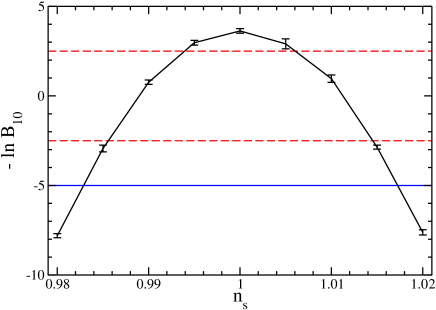
Figure 1: The (negative of the) logarithm of the Bayes factor, $-\ln B_{10}$, as a function of the fiducial value of $n_{{\rm S}}$, where $M_{0}$ is the HZ model and $M_{1}$ is VARYn. The horizontal lines indicate where the comparison becomes ‘strong’ (dashed) and ‘decisive’ (solid) on the Jeffreys’ scale.

Figure 1 shows our main result. At $n_{{\rm S}}=1$, the HZ model is strongly preferred with $\ln B_{10}=-3.6\pm 0.1$. It has a higher evidence since it can fit the data just as well as VARYn and has one less parameter. Once $n_{{\rm S}}$ is far enough away from 1, the HZ fit becomes very poor and the Bayes factor plummets. The speed with which this happens indicates the strength of the experiment.

We see that if the true value lies in the range $0.989<n_{{\rm S}}<1.011$, Bayesian model selection will favour the HZ model, and within the narrower range $0.994<n_{{\rm S}}<1.006$ it will give strong support to that model, though Planck on its own is not powerful enough to be able to decisively favour HZ over VARYn even if HZ is the true case. Only once $n_{{\rm S}}<0.986$ or $n_{{\rm S}}>1.014$ can Planck offer strong evidence against HZ, rapidly becoming decisive as the fiducial value moves away from unity beyond 0.983 or 1.017.

We can contrast these model selection results with those indicated by parameter estimation. Using the same simulated data, we compute the marginalized likelihood of $n_{{\rm S}}$ about $n_{{\rm S}}=1$. This gives a 68% range of $0.995<n_{{\rm S}}<1.004$ and a 95% range of $0.991<n_{{\rm S}}<1.008$, in good agreement with estimates obtained by other authors including the Planck Blue Book. We see this is an explicit example of Lindley’s paradox; there are values of $n_{{\rm S}}$ lying outside the 95 percent confidence region, for which model selection would nevertheless favour the HZ model.

We end by estimating how likely it is that Planck will be able to make a decisive selection between our two models, based on current understanding of the spectral index. We use a variant of Trotta’s ExPO approach T , but with one important distinction; that we use the current model selection position as input, whereas Trotta used the observed likelihood in the VARYn model alone. For simplicity we consider only the marginalized likelihood for $n_{{\rm S}}$ as the starting point rather than marginalizing the model selection outcome over all parameters, but we expect that to make little difference in this case.

According to Parkinson et al. PML , following WMAP3 the balance of probability between HZ and VARYn is 12% to 88% (with some dependence on the choice of data compilation). This makes the important assumption that the models were thought equally likely before the data came along; anyone who thinks otherwise can readily recompute according to their own prejudice. In essence, one can think of the probability distribution for $n_{{\rm S}}$ as being a weighted superposition of the likelihood in the VARYn model plus a delta-function at $n_{{\rm S}}=1$. Trotta omits the delta-function term in his ExPO forecasts.

For the 12% probability that $n_{{S}}$ is actually one, Planck will clearly not find evidence to the contrary, but as we have seen would in that case provide strong evidence for the HZ case. For the remaining probability, we use the marginalized distribution for $n_{{\rm S}}$ as computed in Ref. PML . We find that 7% of the posterior lies in the region $n_{{\rm S}}>0.983$ where even Planck cannot make a decisive verdict. We can therefore conclude that if $n_{{\rm S}}$ is not one, then Planck is expected to provide a decisive verdict against HZ, which WMAP3 has not achieved, but with a small chance it will not.

Trotta T came to the same verdict that Planck is very likely to rule out $n_{{\rm S}}=1$, but using WMAP1 data. However we would not have come to that conclusion using our modification of his approach, as with WMAP1 the model selection verdict put somewhat more than half the probability in the HZ case MPL , and also a significant part of the $n_{{\rm S}}\neq 1$ probability into the indecisive region. Accordingly, at that point we would have said that the most likely outcome of Planck (under the assumption of equal model prior probabilities) was strong support for $n_{{\rm S}}=1$. However, as is always the danger with probabilities, WMAP3 has overturned that conclusion.

III Conclusions

We have carried out a model selection forecast for the Planck satellite, focussing on the scalar spectral index. Such analyses complement the usual parameter error forecasts, and are particularly directed to the question of when one can robustly identify the need for new fit parameters. In particular, we have delineated the values of $n_{{\rm S}}$ for which strong or decisive model comparisons can be carried out. Ruling out $n_{{\rm S}}=1$ is found to be significantly harder than parameter error forecasts suggest.

The recent WMAP3 data have left $n_{{\rm S}}$ poised in an interesting position, where model selection analyses do support parameter estimation conclusions but not yet at a decisive level. Our results show that if $n_{{\rm S}}$ really is different from one, then Planck is very likely to be able to confirm that, but if the HZ case is the true one then even Planck will not be decisive.

- (1) A. R. Liddle and D. H. Lyth, Cosmological inflation and large-scale structure, Cambridge University Press (2000).
- (2) A. R. Liddle, Mon. Not. Roy. Astron. Soc. 351, L49, astro-ph/0401198.
- (3) R. Trotta, astro-ph/0504022.
- (4) P. Mukherjee, D. Parkinson, and A. R. Liddle, Astrophys. J. Lett. 638, L51 (2006), astro-ph/0508461.
- (5) P. Mukherjee, D. Parkinson, P. S. Corasaniti, A. R. Liddle, and M. Kunz, astro-ph/0512484.
- (6) H. Jeffreys H., Theory of Probability, 3rd ed, Oxford University Press (1961).
- (7) D. J. C. MacKay, Information theory, inference and learning algorithms, Cambridge University Press (2003).
- (8) P. Gregory, Bayesian Logical Data Analysis for the Physical Sciences, Cambridge University Press (2005).
- (9) A. Jaffe, Astrophys. J. 471, 24 (1996), astro-ph/9501070; P. S. Drell, T. J. Loredo, and I. Wasserman, Astrophys. J. 530, 593 (2000), astro-ph/9905027; M. V. John and J. V. Narlikar, Phys. Rev. D65, 043506 (2002), astro-ph/0111122; A. Slosar et al., Mon. Not. Roy. Astron. Soc. 341, L29 (2003), astro-ph/0212497; P. J. Marshall, M. P. Hobson, and A. Slosar, Mon. Not. Roy. Astron. Soc. 346, 489 (2003), astro-ph/0307098; T. D. Saini, J. Weller J., and S. L. Bridle, Mon. Not. Roy. Astron. Soc. 348, 603 (2004), astro-ph/0305526; A. Niarchou, A. H. Jaffe, and L. Pogosian, Phys. Rev. D69, 063515 (2004), astro-ph/0308461; B. A. Bassett, P. S. Corasaniti and M. Kunz, Astrophys. J. Lett. 617, L1 (2004), astro-ph/0407364; M. Kunz, R. Trotta, and D. Parkinson, astro-ph/0602378.
- (10) D. N. Spergel et al. (WMAP Collaboration), astro-ph/0603449.
- (11) D. Parkinson, P. Mukherjee, and A. R. Liddle, astro-ph/0605003.
- (12) M. Bridges, A. N. Lasenby, and M. P. Hobson, astro-ph/0511573.
- (13) D. Lindley, Biometrika 44, 187 (1957).
- (14) L. Knox, Phys. Rev. D52, 4307 (1995), astro-ph/9504054.
- (15) A. R. Cooray and W. Hu, Astrophys. J. 534, 533 (2000), astro-ph/9910397.
- (16) M. Kaplinghat, M. Chu, Z. Haiman, G. Holder, L. Knox, and C. Skordis, Astrophys. J. 583, 24 (2003), astro-ph/0207591; A. Lewis, Phys. Rev. D71, 083008 (2005), astro-ph/0502469.
- (17) J. Skilling J., in Bayesian Inference and Maximum Entropy Methods in Science and Engineering, ed. R. Fischer et al., Amer. Inst. Phys., conf. proc., 735, 395 (2004), (available at http://www.inference.phy.cam.ac.uk/bayesys/).