A Bayesian model selection analysis of WMAP3
Abstract
We present a Bayesian model selection analysis of WMAP3 data using our code CosmoNest. We focus on the density perturbation spectral index and the tensor-to-scalar ratio , which define the plane of slow-roll inflationary models. We find that while the Bayesian evidence supports the conclusion that , the data are not yet powerful enough to do so at a strong or decisive level. If tensors are assumed absent, the current odds are approximately 8 to 1 in favour of under our assumptions, when WMAP3 data is used together with external data sets. WMAP3 data on its own is unable to distinguish between the two models. Further, inclusion of as a parameter weakens the conclusion against the Harrison–Zel’dovich case (, ), albeit in a prior-dependent way. In appendices we describe the CosmoNest code in detail, noting its ability to supply posterior samples as well as to accurately compute the Bayesian evidence. We make a first public release of CosmoNest, now available at www.cosmonest.org.
pacs:
98.80.-k astro-ph/0605003I Introduction
The recent three-year results from WMAP wmap3 have provided the first firm indications that the spectral index of primordial density perturbations, , differs from the Harrison–Zel’dovich case . The likelihood function in models with varying suggests that is excluded at around three to four sigma, in cosmologies with no significant tensor contribution to the microwave anisotropies. However, the WMAP team stress that their result, based on a chi-squared per degrees of freedom argument, needs to be checked using the more sophisticated technique of Bayesian model selection Jeff ; MacKay ; Gregory . That is the aim of the present paper, building on our previous analysis of the WMAP first-year data using our code CosmoNest MPL .
We will consider two different scenarios. The first concerns the spectral index alone, under the assumption that there are no primordial gravitational waves (parametrized by the tensor-to-scalar ratio ). As there is presently no indication for gravitational waves, this analysis addresses the question of whether should be considered part of the standard cosmological model. Secondly, we consider the plane of slow-roll inflation models parametrized by and , representing the simplest class of inflation models (for an extensive review, see Ref. LL ). This latter analysis determines the extent to which slow-roll inflation models have benefitted from the new data.
II Bayesian model selection
One of the most important classes of statistical problems in science, and particularly in cosmology, is determining the best fit to data in the case where the underlying model (i.e. the set of parameters to be varied) is unknown. Typically, each parameter represents some physical effect that may influence the data, but one cannot simply include all possible physical effects simultaneously, as the data may be insufficiently constraining and all parameters become undetermined and biases get introduced L04 . In the Bayesian framework, the solution is model selection statistics, which set up a tension between goodness of fit to the data and model complexity. A model selection statistic does not care about the preferred values of the parameters defining the model, but is a property of the model itself, where here ‘model’ means both a choice of the set of parameters to be varied and the prior ranges for those parameters.
A key application of model selection is to provide a robust criterion for judging when data requires the addition of new parameters. Many of the most pressing questions in contemporary cosmology are of this type, such as whether the dark energy density evolves with redshift, or whether primordial gravitational waves exist. For the present data compilation following the WMAP3 announcement, it is the spectral index which is placed in the most interesting position — does WMAP3 convincingly exclude the possibility that is precisely unity, as conjectured by Harrison and by Zel’dovich HZ long before the inflationary mechanism was discovered? In model selection terms, does the improved fit that a varying allows justify its inclusion as an extra variable fit parameter?
One might wonder why we should bother with a model selection analysis of a result which a parameter estimation analysis says is already at three to four sigma level. The answer is that this significance level is exactly where model selection techniques are at their most crucial. It has long been recognized in the statistics community that Bayesian model selection analyses can give results in contradiction with inferences based on ‘number of sigmas’; this is known as Lindley’s ‘paradox’ L and is nicely summarized by Trotta T . Basically, Bayesian inference is inconsistent with the idea that there is a universal threshold, such as 95%, beyond which results should be seen as definitive; instead such a threshold should depend both on the data properties and the prior parameter ranges of the models being compared. The Lindley paradox usually manifests itself for results with significance in the range two to four sigma T , which as it happens is exactly where WMAP3 has placed .
In a full implementation of Bayesian inference, the key statistic is the Bayesian evidence (also known as the marginalized likelihood), which has the literal interpretation of the probability of the data given the model Jeff ; MacKay ; Gregory . According to Bayes theorem, it therefore updates the prior model probability to the posterior model probability. It is simply the average of the likelihood over the prior parameter space. Often, the quantity of interest is the ratio of evidences of two models and , called the Bayes factor and denoted , which indicates how the relative model probabilities have been updated by the data. The evidence has been exploited in a range of cosmological studies ev ; T ; MPL .
Computing the evidence is more challenging than calculating parameter uncertainties, as it requires knowledge of the likelihood throughout the prior parameter volume rather than only in the vicinity of its peak. So far brute force methods such as thermodynamic integration, though accurate, have proved to be computationally very intensive B05 , while approximate information criterion based methods often lead to results which do not agree and hence can be ambiguous L04 ; M06 . We have recently developed an implementation of an algorithm due to Skilling known as Nested Sampling Skilling , which we call CosmoNest MPL , which is able to carry out such calculations efficiently. It is a Monte Carlo method, but not a Markov chain one. We describe the code extensively in Ref. MPL and in the appendices of this article.
In assessing the significance of a model comparison, a useful guide is given by the Jeffreys’ scale Jeff . Labelling as the model with the higher evidence, it rates as ‘not worth more than a bare mention’, as ‘substantial’, ‘strong’ to ‘very strong’ and as ‘decisive’. Note that corresponds to odds of 1 in about 150, and to odds of 1 in 13.
III Application to WMAP3
Throughout we use a data compilation of the WMAP3 TT, TE and EE anisotropy power spectrum data wmap3 , together with higher CMB temperature power spectrum data from ACBAR ACBAR , CBI CBI , VSA VSA , and Boomerang 2003 boom , and also matter power spectrum data from SDSS SDSS and 2dFGRS 2df . Following the approach of Ref. Peiris , we use the updated beam error module, and do not marginalize over the amplitude of SZ fluctuations. For the higher CMB data, we neglect those bands that overlap in range with WMAP (as in Ref. wmap3 ), so that they can be treated as independent measurements.
The prior ranges for the other parameters were chosen as in Ref. MPL : , , , , and . Here is a measure of the sound horizon at decoupling, and the other symbols have their usual meaning.
When we quote Bayes factors, model is always taken to be the Harrison–Zel’dovich case. We normalize to this case, which means positive numbers indicate models preferred against this case.
III.1 The spectral index
For the spectral index , we will throughout assume a prior range , as in Refs. B05 ; MPL . The model selection results presented for must therefore be understood in light of this prior. As the allowed regions are well contained within this prior, it is trivial to recompute the Bayes factor if this range is extended; e.g. if it is doubled then is reduced by .
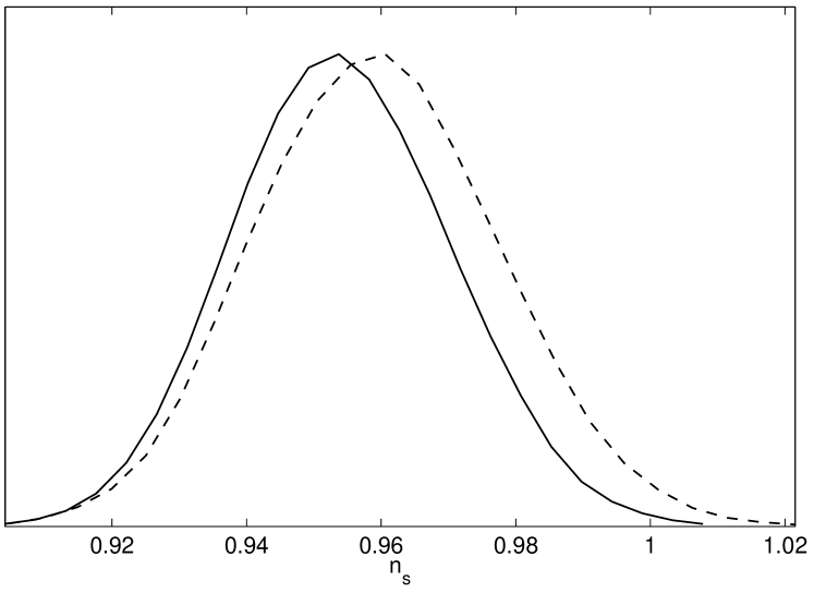
Qualitative understanding of our results can be obtained from studying the marginalized distributions for , shown in Fig. 1, obtained using CosmoNest. For reasons explained later, we did not include marginalization over the SZ effect in obtaining these likelihoods, which shifts them somewhat towards as compared to those of the WMAP team wmap3 . A rapid guide to the expected result can be obtained by employing a gaussian approximation to the marginalized posterior distribution for . As shown by Trotta T , the Bayes factor can be computed in this approximation as a function of , being the ‘number of sigmas’ of the putative detection, and the information content which measures the reduction of the allowed parameter volume between the prior and posterior (where is the prior width and the standard deviation of the posterior). For WMAP3 alone and our choice of prior and . Employing Eq. (18) of Ref. T yields the estimate , i.e. the varying model is preferred but only very mildly. However, this expression assumes that the gaussian form holds quite far into its tail, which may not be valid, and so we proceed to results from the full numerical calculation (which we anyway had to do to obtain these marginalized likelihoods as a by-product, as explained in Appendix B).
Using CosmoNest, we ran the Harrison–Zel’dovich (HZ) and spectral index cases () to find the difference in evidence for WMAP3, with and without the external CMB and large-scale structure data sets. We found that using WMAP alone, , in agreement with the estimate above. However, when the extra data sets are included, , which is substantial but not strong evidence for the necessity of as an extra parameter. The results are given in Table 1.
The difference of 1.65 in between the two datasets can be understood simply from the marginalized likelihoods shown in Fig. 1. Although the curves are similar near the peaks, and the maximum likelihood value has shifted only by about , the difference in the mean and more importantly the variance have a large effect in the tails. The probability of the value is about 4 times smaller in the WMAP+all case, which would, all else being considered equal, translate into a change of in explaining most of the difference. Nevertheless, this shift is not particularly significant on the Jeffreys’ scale.
III.2 The inflationary plane
A non-zero value of is commonly interpreted as a strong indication in favour of inflation. However slow-roll inflationary models predict not just a non-zero , but also a non-zero value for the tensor-to-scalar ratio . A proper model comparison motivating inflation should therefore examine not the spectral index model but the two-parameter extension of HZ into the – plane. There is no simple way to make an estimate of the outcome in this case.
At this point we run into the issue of the choice of prior for . While it is uncontroversial to choose a uniform prior for , whose value is more or less known, is instead a parameter whose order-of-magnitude is currently unknown (sometimes called a ‘scale’ parameter). We will consider two possibilities. The first, Case 1, is that has a uniform prior in the range , which is the assumption used by Spergel et al. wmap3 for parameter estimation. The second, Case 2, considers the Jeffreys’ prior which states that for scale parameters the prior should be uniform in rather than . For the problem to be well-defined this needs to be cut off at both ends. We use the same upper limit, and as a lower limit take the smallest conceivable inflation scale of the electroweak scale, which would yield (where is the energy density). The prior range is therefore . Results are shown in Table 1.
| Datasets | Model | |
| WMAP only | HZ | |
| WMAP + all | HZ | |
| + (uniform prior) | ||
| + (log prior) |
For Case 1, CosmoNest calculations indicate of . The large amount of unused prior parameter space in the – plane means that this model is somewhat disfavoured as compared to HZ.
For Case 2, a calculation is not in fact really necessary, since the vast majority of the prior space lies in the region where is observationally negligible, and hence generates the same likelihood as a model where the spectral index alone varies. We confirm this explicitly by computing evidence over a limited range and extrapolating the result down to .
We conclude therefore that the evidence in the inflationary plane does carry significant prior dependence, bracketted by the values we have found under Case 1 and Case 2. Given the present shape of the likelihood, the evidence for the inflation model will not be as large as for the spectral index model under any prior choice, and may be significantly less. For a uniform prior on , the inflation model is actually rated below Harrison–Zel’dovich.
III.3 Systematic effects
The evidence computation we have described takes into account only statistical uncertainties. However one should also consider the possible effect of systematic uncertainties, and there are some indications that these are present at a level which would have some impact on our conclusions, despite the very careful job that the WMAP team have done. We highlight some of these issues here.
There is some effect from the precise choice of dataset used. All the dataset combinations quoted in Ref. wmap3 give very similar constraints on , though none corresponds precisely to the dataset compilation we are employing. Curiously though, the dataset WMAP+all on the LAMBDA archive,111http://lambda.gsfc.nasa.gov which adds two supernovae datasets to our compilation, gives an value about one-sigma lower than any other dataset quoted, which would be expected to lead to a stronger result for the Bayes factor. However it is puzzling that this data compilation gives a lower (and optical depth ) than do any of the separate datasets from which it is compiled.
There is some uncertainty in how to treat the Sunyaev–Zel’dovich effect and gravitational lensing. The WMAP team allow only for the former, while Lewis has argued Lewis that the two effects are of the same order, and nearly cancel, at least as regards their effect on , and that it is better to ignore both than to include only one. Accordingly we have not included the SZ correction, which increases as compared to the WMAP3 analysis.
Another subtlety concerns the modelling of the beam. As discussed in Ref. Peiris there are different options for doing this, which appear to have a slight effect on the constraint on . We have followed the procedure described in that paper, rather than that of the main WMAP3 papers wmap3 .
Yet more uncertainty surrounds the modelling of the recombination process. According to Ref. DG , inclusion of additional two-photon decays leads to significant differences as compared to the standard RECFAST treatment used in the WMAP papers. If confirmed, this is perhaps not too important for WMAP, but would certainly matter at Planck sensitivity (Antony Lewis, private communication).
Also, the reionization optical depth and are correlated. The constraint on comes mainly from the estimate of the power in the low multipoles of CMB polarization. Substantial foregrounds are present in polarization data, so that their removal using just the frequency information gathered by WMAP can be tricky. Foreground subtraction uncertainties could therefore affect and hence .
Finally, we note that the inclusion of Lyman alpha power spectrum data (not used in the WMAP3 papers) seems to have a marginally significant effect. According to the analysis of Ref. SSM , inclusion of this data shifts upwards by around one-sigma while leaving the uncertainty unchanged. Similar results are obtained in Ref. VHL though the trend is less clear as they round their quoted results at the second decimal place.
While individually none of the above would have a very major effect on model selection conclusions, that there are so many clearly urges caution in interpretting a result whose statistical significance remains rather marginal.
IV Conclusions
We have carried out a Bayesian model selection analysis of WMAP3 data, as advocated by the WMAP team. We have found that WMAP3 data do indeed give support for a varying spectral index when combined with other data, with the Bayes factor compared to the Harrison–Zel’dovich spectrum being approximately . According to the Jeffreys’ scale, this should be regarded as significant, but neither strong nor decisive. It corresponds to probabilistic odds of about 8 to 1 against the Harrison–Zel’dovich model (i.e. the chance that is equal to one is about that of tossing a coin three times and them all being heads). WMAP3 alone does not provide any discrimination between the models.
In computing our numbers, we have assumed throughout that the prior model probabilities are equal, so that models are regarded as equally likely before the data came along. Anyone who prefers to make an alternative assumption is welcome to do so, and can readily follow the consequences using the evidence numbers we have supplied. For instance, a perfectly plausible standpoint might be that since inflation is a physical model, its predictions should be taken more seriously than pure HZ which is motivated only by symmetry considerations. Hence its prior model probability should be greater, perhaps tipping the post-data odds decisively against HZ. Readers are quite welcome to take that viewpoint, but should bear in mind that their conclusion then derives from a mixture of the data and their prior prejudice. From the data alone, the situation remains to be decisively resolved.
In a companion paper PLMP , we forecast the abilities of the Planck satellite to resolve this situation, in light of the WMAP3 results.
Acknowledgements.
The authors were supported by PPARC. We thank Mike Hobson, Martin Kunz, Antony Lewis, Cédric Pahud, Hiranya Peiris, Douglas Scott, John Skilling, and Roberto Trotta for helpful discussions. We acknowledge use of the UK National Cosmology Supercomputer (COSMOS) funded by Silicon Graphics, Intel, HEFCE and PPARC.Appendix A The Nested Sampling Algorithm
Our implementation of the Nested Sampling algorithm is described in Ref. MPL . To summarize, the algorithm (as first developed in Ref. Skilling ) recasts the problem of calculating the evidence as a one-dimensional integral in terms of the remaining prior mass , where . So the integral is transformed
| (1) |
where is the likelihood . The algorithm samples the prior a large number of times, assigning a ‘prior mass’ probabilistically to each sample. The samples are ordered by likelihood, and the integration follows as the sum of the sequence,
| (2) |
The scheme is illustrated in Figure 2.
In order to compute the integral accurately the prior mass is logarithmically sampled. We start by randomly placing points uniformly in the prior space, where in a typical cosmological application . We then iteratively discard the lowest likelihood point , replacing it with a new point uniformly sampled from the remaining prior mass (i.e. with likelihood ). Each time a point is discarded the prior mass remaining shrinks by a factor that is known probabilistically, and the evidence is incremented accordingly. In this way the algorithm works its way towards the higher likelihood regions.
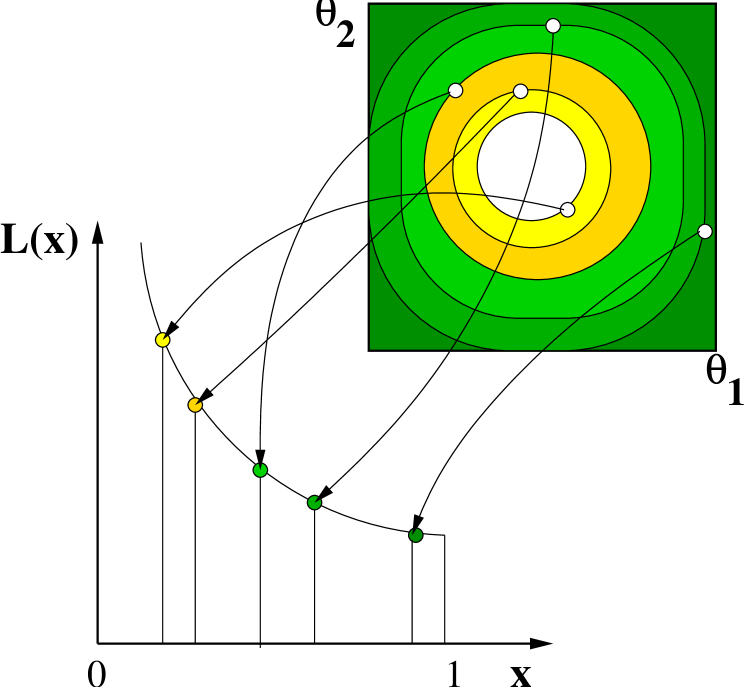
As the remaining prior mass shrinks by orders of magnitude, the challenging part is to find an efficient way to draw new points from the remaining prior volume. We do this by using the remaining points at each stage to define an ellipsoid that encompasses the extremes of the points and is aligned with their principal axes. The ellipsoid is expanded by a constant enlargement factor, in order to allow for the iso-likelihood contours not being exactly elliptical, as well as to take in the edges. New points are then selected uniformly within the expanded ellipse until one has a likelihood exceeding the old minimum.
The process is terminated when the integral has been computed to desired accuracy (see Ref. MPL ). In the end the evidence contributed by the points remaining is added to the accumulated evidence.
The method is general, and the effects of topology and dimensionality are implicitly built into it.
Appendix B CosmoNest
The Cosmological Monte Carlo code (CosmoMC) developed by Lewis and Bridle Lewis:2002 was created to perform an exploration of the cosmological parameter space, through the Monte Carlo Markov Chain process (for an overview of MCMC methods see Ref. MCMC ). While it is most commonly used with the Metropolis–Hastings algorithm, other sampling algorithms (such as Gibbs Sampling and Slice Sampling) can easily be implemented. The Nested Sampling algorithm can be considered as just another Monte Carlo sampling algorithm. The important difference is that the generation of a chain, which in this case is not a Markov chain, is ancillary to its primary purpose of calculating the evidence accurately.
The Cosmological Nested Sampling code (CosmoNest) we have developed is an additional module that works as part of CosmoMC.
B.1 Evidence evaluation
CosmoMC has a ‘memory’ of only one point: the algorithm needs only to know where it is in order to decide where to go next. CosmoNest needs to know about the point it is discarding, but must also hold in its memory all the other live points, as well as knowing how far through the prior mass it has progressed and what value of the evidence () it has accumulated. The output of a CosmoNest run consists of the set of discarded minimum likelihood points, along with their value, their likelihood, and total accumulated evidence to that point.
CosmoMC runs multiple chains for two purposes: increasing the speed of generating samples, and as a way of estimating the extent to which the chains have explored the parameter space (the Gelman–Rubin statistic). Here we run multiple iterations of CosmoNest to obtain an estimate of the uncertainty in the computed evidence.
B.2 Posterior samples
The sequence of discarded points from the Nested Sampling process is similar to the Markov chain produced by an MCMC process with one important difference: the MCMC points are sampled from the posterior whereas the Nested Sampling points are sampled from the prior with a known distribution in . With the appropriate weightings, the ‘chain’ of discarded points (distributed uniformly in ) plus the remaining live points (distributed uniformly in within the remaining volume) can be used to construct the posterior probability distribution of the parameters, as outlined in Ref. Skilling .

To summarize, from Bayes’ theorem
| (3) |
where is the posterior probability of a parameter point given data , is the likelihood and the prior. So for an element in the chain of discarded points, the posterior weighting is
| (4) |
where is the prior mass associated with that particular point. The points finally remaining also need to be included to avoid undersampling the centre of the distribution. They are taken as uniformly sampling the remainder of the prior space.
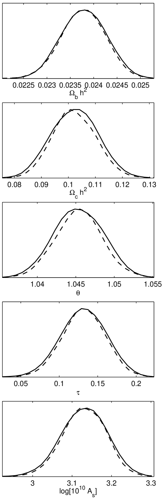
Figure 3 shows as an example of the posterior weights assigned in a particular run. The early points have negligible weight as their likelihood is low, and the late ones because the prior mass per point becomes small. We see that in this case the live points have to be included to properly sample the centre of the distribution. The fractional contribution from live points can be reduced by running the code for longer. The structure of these weights should be contrasted with Metropolis–Hastings where all samples have integer weights (values greater than one accruing when new samples are rejected and instead the original sample duplicated).
Using this method we can reconstruct the posterior samples and compare to similar results from standard Metropolis–Hastings MCMC. We illustrate this in Fig. 4. Posteriors obtained from the two methods are in good agreement.
B.3 The information
The information is defined as (minus) the logarithm of the amount the posterior is compressed inside the prior Skilling . It is easy to compute from the posterior samples once the evidence has been calculated:
| (5) |
The uncertainty on a single estimate of the evidence is dominated by the Poisson uncertainty in the number of steps (replacements) to reach the bulk of the posterior. This is given by . For the priors we have been considering , and given our choice of , this uncertainty turns out to be 0.15 to 0.2.
B.4 Public code release
The CosmoNest code is now freely available for public use, and can be
downloaded from www.cosmonest.org. Its use requires a working
installation of the CosmoMC package of Lewis and Bridle
Lewis:2002 .
References
- (1) D. N. Spergel et al. (WMAP Collaboration), astro-ph/0603449; G. Hinshaw et al. (WMAP Collaboration), astro-ph/0603451; L. Page et al. (WMAP Collaboration), astro-ph/0603450.
- (2) H. Jeffreys, Theory of Probability, 3rd ed, Oxford University Press (1961).
- (3) D. J. C. MacKay, Information theory, inference and learning algorithms, Cambridge University Press (2003).
- (4) P. Gregory, Bayesian Logical Data Analysis for the Physical Sciences, Cambridge University Press (2005).
- (5) P. Mukherjee, D. Parkinson, and A. R. Liddle, Astrophys. J. Lett. 638, L51 (2006), astro-ph/0508461.
- (6) A. R. Liddle and D. H. Lyth, Cosmological inflation and large-scale structure, Cambridge University Press (2000).
- (7) A. R. Liddle, Mon. Not. Roy. Astron. Soc. 351, L49, astro-ph/0401198.
- (8) R. Harrison, Phys. Rev. D1, 2726 (1970); Ya. B. Zel’dovich, Mon. Not. Roy. Astron. Soc. 160, 1p (1972).
- (9) D. Lindley, Biometrika 44, 187 (1957).
- (10) R. Trotta, astro-ph/0504022.
- (11) A. Jaffe, Astrophys. J. 471, 24 (1996), astro-ph/9501070; P. S. Drell, T. J. Loredo, and I. Wasserman, Astrophys. J. 530, 593 (2000), astro-ph/9905027; M. V. John and J. V. Narlikar, Phys. Rev. D65, 043506 (2002), astro-ph/0111122; A. Slosar et al., Mon. Not. Roy. Astron. Soc. 341, L29 (2003), astro-ph/0212497; T. D. Saini, J. Weller, and S. L. Bridle, Mon. Not. Roy. Astron. Soc. 348, 603 (2004), astro-ph/0305526; P. J. Marshall, M. P. Hobson, and A. Slosar, Mon. Not. Roy. Astron. Soc. 346, 489 (2003), astro-ph/0307098; A. Niarchou, A. H. Jaffe, and L. Pogosian, Phys. Rev. D69, 063515 (2004), astro-ph/0308461; B. A. Bassett, P. S. Corasaniti and M. Kunz, Astrophys. J. Lett. 617, L1 (2004), astro-ph/0407364; M. Bridges, A. N. Lasenby, and M. P. Hobson, astro-ph/0511573; P. Mukherjee, D. Parkinson, P. S. Corasaniti, A. R. Liddle, and M. Kunz, astro-ph/0512484; M. Kunz, R. Trotta, and D. Parkinson, astro-ph/0602378.
- (12) M. Beltrán, J. Garcia-Bellído, J. Lesgourgues, A. R. Liddle, and A. Slosar, Phys. Rev. D71, 063532 (2005), astro-ph/0501477.
- (13) J. Magueijo and R. D. Sorkin, astro-ph/0604410.
- (14) J. Skilling , in Bayesian Inference and Maximum Entropy Methods in Science and Engineering, ed. R. Fischer et al., Amer. Inst. Phys., conf. proc., 735, 395 (2004), (available at http://www.inference.phy.cam.ac.uk/bayesys/).
- (15) C. L. Kuo et al., Astrophys. J. 600, 32 (2004), astro-ph/0212289.
- (16) T. J. Pearson et al., Astrophys. J. 591, 556 (2003), astro-ph/0205388.
- (17) C. Dickinson et al., Mon. Not. Roy. Astron. Soc. 353, 732 (2004), astro-ph/0402498.
- (18) W. C. Jones et al., astro-ph/0507494.
- (19) M. Tegmark et al., Astrophys. J. 606, 702 (2004), astro-ph/0310725.
- (20) W. Percival et al., Mon. Not. Roy. Astron. Soc. 327, 1297 (2001), astro-ph/0105252.
- (21) H. Peiris and R. Easther, astro-ph/0603587.
- (22) A. Lewis, astro-ph/0603753.
- (23) V. K. Dubrovich and S. I. Grachev, Astron. Lett. 31, 359 (2005), astro-ph/0501672.
- (24) U. Seljak, A. Slosar, and P. McDonald, astro-ph/0604335.
- (25) M. Viel, M. G. Haehnelt, and A. Lewis, astro-ph/0604310.
- (26) C. Pahud, A. R. Liddle, P. Mukherjee, and D. Parkinson, astro-ph/0605004.
- (27) A. Lewis and S. Bridle, Phys. Rev. D 66, 103511 (2002), astro-ph/0205436, code available from http://cosmologist.info/cosmomc.
- (28) W. R. Gilks, S. Richardson, and D. J. Speigelhalter, Markov Chain Monte Carlo in Practice, Chapman and Hall, London (1996); D. S. Sivia, Bayesian Data Analysis, Clarendon Press, Oxford (1996).