A Two-Zone Model for Type I X-ray Bursts on Accreting Neutron Stars

Abstract

We construct a two-zone model to describe hydrogen and helium burning on the surface of an accreting neutron star and use it to study the triggering of type I X-ray bursts. Although highly simplified, the model reproduces all of the bursting regimes seen in the more complete global linear stability analysis of Narayan & Heyl (2003), including the regime of delayed mixed bursts. The results are also consistent with observations of type I X-ray bursts. At low accretion rates $\dot{M}/\dot{M}_{\mathrm{Edd}}\lesssim 0.1$, thermonuclear helium burning via the well-known thin-shell thermal instability triggers bursts. As $\dot{M}$ increases, however, the trigger mechanism evolves from the fast thermal instability to a slowly growing overstability involving both hydrogen and helium burning. The competition between nuclear heating via the $\beta$-limited CNO cycle and the triple-$\alpha$ process on the one hand, and radiative cooling via photon diffusion and emission on the other hand, drives oscillations with a period approximately equal to the hydrogen-burning timescale. If these oscillations grow, the gradually rising temperature at the base of the helium layer eventually provokes a thin-shell thermal instability and hence a delayed mixed burst. This overstability closely resembles the delayed mixed bursts of Narayan & Heyl. For $\dot{M}/\dot{M}_{\mathrm{Edd}}\gtrsim 0.25$ there is no instability or overstability, and there are no bursts. Nearly all other theoretical models, including detailed time-dependent multi-zone calculations, predict that bursts should occur for all $\dot{M}/\dot{M}_{\mathrm{Edd}}\lesssim 1$, in conflict with both our results and observations. We suggest that this discrepancy arises from the assumed strength of the hot CNO cycle breakout reaction ¹⁵O($\alpha$,$\gamma$)¹⁹Ne in these other models. That observations agree much better with the results of Narayan & Heyl and our two-zone model, both of which neglect breakout reactions, may imply that the true ¹⁵O($\alpha$,$\gamma$)¹⁹Ne cross section is much smaller than assumed in previous investigations.

1. Introduction

Type I X-ray bursts are thermonuclear explosions that occur on the surfaces of accreting neutron stars (Babushkina et al., 1975; Grindlay & Heise, 1975; Grindlay et al., 1976; Belian et al., 1976; Woosley & Taam, 1976; Joss, 1977; Maraschi & Cavaliere, 1977; Lamb & Lamb, 1977, 1978). They are triggered by unstable helium or hydrogen burning (for reviews, see Lewin et al., 1993, 1995; Cumming, 2004; Strohmayer & Bildsten, 2006). For a wide range of accretion rates, the basic physics of the burst onset is that of the well-known thin-shell thermal instability (Schwarzschild & Härm, 1965; Hansen & van Horn, 1975), which operates as follows. In equilibrium, the energy that is generated by nuclear burning is exactly balanced by the outward diffusion of photons coupled with radiation from the stellar surface. If the nuclear reaction rates are sufficiently temperature-sensitive, a positive temperature perturbation causes the nuclear energy generation rate to increase faster than the rate at which the stellar surface can cool, causing a thermonuclear runaway and hence a type I X-ray burst. The physics of this instability can be described quite well with a simple one-zone model (Fujimoto et al., 1981; Paczyński, 1983a; Bildsten, 1998; Cumming & Bildsten, 2000). If the amount of accreted matter needed to ignite a burst were roughly independent of the accretion rate $\dot{M}$, as suggested by simple models, one would expect the recurrence time $t_{\mathrm{rec}}$ to vary as $\dot{M}^{-1}$. This is in reasonable agreement with observations for a range of $\dot{M}\lesssim 0.1\dot{M}_{\mathrm{Edd}}$, where $\dot{M}_{\mathrm{Edd}}$ denotes the mass accretion rate at which the accretion luminosity is equal to the Eddington limit. However, for $0.1\lesssim\dot{M}/\dot{M}_{\mathrm{Edd}}\lesssim 0.3$, observations show that $t_{\mathrm{rec}}$ increases with increasing $\dot{M}$, and bursts are found to cease altogether for $\dot{M}/\dot{M}_{\mathrm{Edd}}\gtrsim 0.3$ (van Paradijs et al., 1979, 1988; Cornelisse et al., 2003; Remillard et al., 2006). Moreover, for $0.1\lesssim\dot{M}/\dot{M}_{\mathrm{Edd}}\lesssim 0.3$, most of the accreted matter appears to burn stably between consecutive bursts (van Paradijs et al., 1988; in’t Zand et al., 2003). Simple thin-shell thermal instability models, on the other hand, predict that bursts should occur for all $\dot{M}/\dot{M}_{\mathrm{Edd}}\lesssim 1$ and that $t_{\mathrm{rec}}$ should decrease monotonically with increasing $\dot{M}$.

Narayan & Heyl (2003, hereafter NH03) developed a global linear stability analysis of the accreted nuclear fuel on the surface of a neutron star. Unlike thin-shell thermal instability models, for which one assumes that purely thermal perturbations trigger bursts, NH03’s analysis was quite general and made no assumptions as to the trigger mechanism. Apart from confirming the standard thermal instability for $\dot{M}/\dot{M}_{\mathrm{Edd}}\lesssim 0.1$, NH03 discovered a new regime of unstable nuclear burning for $0.1\lesssim\dot{M}/\dot{M}_{\mathrm{Edd}}\lesssim 0.3$ that they referred to as “delayed mixed bursts.” This regime reproduced the increase in $t_{\mathrm{rec}}$ with increasing $\dot{M}$ seen in observations, as well as the occurrence of considerable stable burning between successive bursts. It also predicted the absence of bursts for $\dot{M}/\dot{M}_{\mathrm{Edd}}\gtrsim 0.3$, again in agreement with observations. Recently, Cooper & Narayan (2005) and Cooper et al. (2006) have suggested that the stable burning that precedes delayed mixed bursts is crucial for the production of the carbon fuel needed to trigger superbursts (for reviews of superbursts, see Kuulkers, 2004; Cumming, 2005), since only stable nuclear burning can produce carbon in sufficient quantities (Schatz et al., 1999, 2001, 2003; Koike et al., 2004; Woosley et al., 2004; Fisker et al., 2005).

It is perhaps not surprising that a global linear stability analysis is able to reproduce type I X-ray burst observations better than simple thin-shell thermal instability models. However, the fact that the results of all time-dependent multi-zone models with large reaction networks conflict with observations as well (Ayasli & Joss, 1982; Taam et al., 1996; Fisker et al., 2003; Heger et al., 2005) is much more problematic. Like the global linear stability analysis, these latter models include no preconceived instability criteria. Therefore, they should in principle be able to reproduce the regime of delayed mixed bursts and the absence of bursts for $\dot{M}/\dot{M}_{\mathrm{Edd}}\gtrsim 0.3$, as observed in nature. The disagreement between the predictions of time-dependent multi-zone burst models and the global linear stability analysis of NH03 suggests that some crucial aspect of the physics is different between the two. Understanding this discrepancy is of fundamental importance in the study of type I X-ray bursts.

While the global linear stability analysis of NH03, with its identification of the delayed mixed burst regime, succeeded in reproducing several puzzling observations of bursts, unfortunately, the complexity of the model and the absence of a specific stability criterion make it difficult to understand the basic physics of delayed mixed bursts. To rectify this situation, we construct here a simple two-zone model that reproduces all of the basic features of the global analysis. We begin in §2 with a derivation of our model. In §3, we discuss the equilibria of the model and analyze their stability as a function of accretion rate. We then integrate the equations that govern the model and use the results in §4 to explain the physics of the onset of delayed mixed bursts. We discuss our results in §5, and we conclude in §6.

2. The Model

We assume that matter accretes spherically onto a neutron star of gravitational mass $M=1.4M_{\odot}$ and areal radius $R=10\,\mathrm{km}$ at an accretion rate per unit area $\dot{\Sigma}$ as measured in the local frame of the accreted plasma. We consider all physical quantities to be functions of the column depth $\Sigma$, which we define as the rest mass of the accreted matter as measured from the stellar surface divided by $4\pi R^{2}$. We denote the Eulerian time and spatial derivatives as $\partial/\partial t$ and $\partial/\partial\Sigma$, respectively, and we denote the Lagrangian derivative following a parcel of matter as $D/Dt$, where $D/Dt=\partial/\partial t+\dot{\Sigma}\partial/\partial\Sigma$. We describe the composition of the matter by the hydrogen mass fraction $X$, helium mass fraction $Y$, and heavy element fraction $Z=1-X-Y$. The mass fractions at $\Sigma=0$, $X_{0}$, $Y_{0}$, and $Z_{0}$, are those of the accreted plasma. In this work, we assume that all heavy elements are CNO and that the composition of the accreted matter is that of the Sun: $\xout{=}0.7$, $Y_{0}=0.28$, $Z_{0}=0.02$.

The following set of four partial differential equations governs the thermal structure and time evolution of the material (e.g., NH03; see Table 1 of that paper for the definitions of the various symbols):

$$\frac{\partial T^{4}}{\partial\Sigma}=\frac{3\kappa F}{ac},$$ (1)

$$\frac{\partial F}{\partial\Sigma}=T\frac{Ds}{Dt}-(\epsilon_{\mathrm{H}}+\epsilon_{\mathrm{He}}),$$ (2)

$$\frac{DX}{Dt}=-\frac{\epsilon_{\mathrm{H}}}{E^{*}_{\mathrm{H}}},$$ (3)

$$\frac{DZ}{Dt}=\frac{\epsilon_{\mathrm{He}}}{E^{*}_{\mathrm{He}}}.$$ (4)

Since we are interested in developing a simple model that avoids unnecessary details, we follow Bildsten (1998) and set the opacity to a constant value, $\kappa=0.4\kappa_{\mathrm{es}}=0.136$ $\mathrm{cm}^{2}\,\mathrm{g}^{-1}$, where $\kappa_{\mathrm{es}}$ is the Thomson scattering opacity. We assume that a nondegenerate, ideal gas supplies the pressure $P$, which is a good approximation for the shallow column depths we consider in this work. The specific entropy $s$ is in general a function of both $T$ and $P=g\Sigma$, and so

$$T\frac{Ds}{Dt}=C_{\mathrm{p}}\frac{\partial T}{\partial t}+C_{\mathrm{p}}\dot{\Sigma}\left(\frac{\partial T}{\partial\Sigma}-\frac{T}{\Sigma}\nabla_{\mathrm{ad}}\right),$$ (5)

where we set the specific heat at constant pressure $C_{\mathrm{p}}=5k_{\mathrm{B}}/2m_{\mathrm{p}}$ for an assumed mean molecular weight $\mu=1$, and $\nabla_{\mathrm{ad}}\equiv(\partial\ln T/\partial\ln\Sigma)_{s}=2/5$ for an ideal gas. We ignore the terms $\propto\dot{\Sigma}$ for reasons we will give in §3 (this is a standard approximation in most one-zone models of type I X-ray bursts, e.g., Bildsten, 1998; Cumming & Bildsten, 2000) although we have done calculations with these terms included, and we have verified that they are not important. Thus, equation (2) becomes

$$\frac{\partial F}{\partial\Sigma}=C_{\mathrm{p}}\frac{\partial T}{\partial t}-(\epsilon_{\mathrm{H}}+\epsilon_{\mathrm{He}}).$$ (6)

The usual one-zone approach to type I X-ray bursts (Fujimoto et al., 1981; Paczyński, 1983a; Bildsten, 1998; Cumming & Bildsten, 2000) focuses primarily on helium burning, for which a single zone is adequate. Several authors have introduced more elaborate two-zone models of type I X-ray bursts (Buchler & Perdang, 1979; Barranco et al., 1980; Regev & Livio, 1984; Livio & Regev, 1985; Yasutomi, 1987), but these models usually include only helium burning, and all of the nuclear burning is confined to a single zone. José et al. (1993) present a two-zone model of thermonuclear burning on accreting white dwarfs that includes both hydrogen and helium burning, but the two fuels are forced to burn in separate zones by construction. This approximation is too severe for realistic modeling of type I X-ray bursts. The global linear stability analysis of NH03 clearly shows that the interaction between hydrogen and helium burning plays a key role in delayed mixed bursts. Motivated by this, we describe in this paper a new model with the following two zones: (i) a zone that begins at the surface of the star, where $\Sigma=0$, and extends to the depth $\Sigma_{\mathrm{H}}$ at which hydrogen is depleted via nuclear burning, and (ii) a zone that begins at $\Sigma_{\mathrm{H}}$ and extends to the depth $\Sigma_{\mathrm{He}}$ at which helium is depleted via nuclear burning. Hydrogen, helium, and CNO are all present in zone (i), while only helium and CNO are present in zone (ii). Furthermore, we include both hydrogen and helium burning in zone (i), but we include only helium burning in zone (ii) since hydrogen is not present. Note that, in our model, hydrogen fully depletes before all of the helium burns by construction, so that $\Sigma_{\mathrm{He}}>\Sigma_{\mathrm{H}}$. This condition is satisfied over the entire range of $\dot{\Sigma}$ of interest in this work. We discuss the case for which $\Sigma_{\mathrm{He}}<\Sigma_{\mathrm{H}}$ in §5. We make the simplification that all thermonuclear processes within a zone take place at the bottom of that zone. Equation (2) thus implies that the flux $F$ in a particular zone is a constant with respect to $\Sigma$, and so $T^{4}$ varies linearly with $\Sigma$ within each zone (see equation 1).

In the simplest one-zone models, all parameters of the matter are taken to be constant within the zone. Clearly this prescription is a gross simplification, for in reality the physical parameters $X$, $Y$, $Z$, $T$, and $F$ vary smoothly as functions of $\Sigma$. In order to improve the accuracy of our model, we assume linear profiles with respect to depth of the various quantities of interest (except $F$). Thus we take

$$X(\Sigma,t)=\left\{\begin{array}[]{ll}\xout{(}1-\Sigma/\Sigma_{\mathrm{H}}),&\Sigma<\Sigma_{\mathrm{H}}\\ 0,&\Sigma>\Sigma_{\mathrm{H}},\\ \end{array}\right.$$ (7)

$$Z(\Sigma,t)=\left\{\begin{array}[]{lll}Z_{0}+(Z_{\mathrm{H}}-Z_{0})(\Sigma/\Sigma_{\mathrm{H}}),&\Sigma<\Sigma_{\mathrm{H}}\\ Z_{\mathrm{H}}+(1-Z_{\mathrm{H}})(\Sigma-\Sigma_{\mathrm{H}})/\Delta\Sigma,&\Sigma_{\mathrm{H}}<\Sigma<\Sigma_{\mathrm{He}}\\ 1,&\Sigma>\Sigma_{\mathrm{He}},\\ \end{array}\right.$$ (8)

$$T^{4}(\Sigma,t)=\left\{\begin{array}[]{lll}T_{\mathrm{H}}^{4}(\Sigma/\Sigma_{\mathrm{H}}),&\Sigma<\Sigma_{\mathrm{H}}\\ T_{\mathrm{H}}^{4}+(T_{\mathrm{He}}^{4}-T_{\mathrm{H}}^{4})(\Sigma-\Sigma_{\mathrm{H}})/\Delta\Sigma,&\Sigma_{\mathrm{H}}<\Sigma<\Sigma_{\mathrm{He}}\\ T_{\mathrm{He}}^{4},&\Sigma>\Sigma_{\mathrm{He}},\\ \end{array}\right.$$ (9)

$$F(\Sigma,t)=\left\{\begin{array}[]{lll}F_{\mathrm{H}},&\Sigma<\Sigma_{\mathrm{H}}\\ F_{\mathrm{He}},&\Sigma_{\mathrm{H}}<\Sigma<\Sigma_{\mathrm{He}}\\ 0,&\Sigma>\Sigma_{\mathrm{He}},\\ \end{array}\right.$$ (10)

where

$$Z_{\mathrm{H}}\equiv Z(\Sigma_{\mathrm{H}}),\,\,\,\,\,T_{\mathrm{H}}\equiv T(\Sigma_{\mathrm{H}}),\,\,\,\,\,T_{\mathrm{He}}\equiv T(\Sigma_{\mathrm{He}}),$$ (11)

$$\Delta\Sigma\equiv\Sigma_{\mathrm{He}}-\Sigma_{\mathrm{H}},$$ (12)

and the five quantities $\Sigma_{\mathrm{H}}$, $Z_{\mathrm{H}}$, $T_{\mathrm{H}}$, $\Sigma_{\mathrm{He}}$, and $T_{\mathrm{He}}$ are functions of time. Note that equation (9) is exact for the aforementioned simplifications of constant opacity and constant flux within a zone. Figure 1 shows a pictorial representation of the model. For simplicity, we assume that the flux $F$ entering the bottom of the helium-burning zone from the stellar interior is zero. Integrating equation (1) gives

$$F_{\mathrm{H}}=\frac{acT_{\mathrm{H}}^{4}}{3\kappa\Sigma_{\mathrm{H}}},$$ (13)

$$F_{\mathrm{He}}=\frac{ac(T_{\mathrm{He}}^{4}-T_{\mathrm{H}}^{4})}{3\kappa\Delta\Sigma}.$$ (14)

Figure 1.— A schematic representation of how the composition, temperature, and flux vary as a function of column depth in the proposed two-zone model. , $Y_{0}$, and $Z_{0}$ denote the hydrogen, helium, and CNO mass fractions of the accreted plasma, respectively. Zone (i) extends from $\Sigma=0$ to $\Sigma=\Sigma_{\mathrm{H}}$, and zone (ii) extends from $\Sigma=\Sigma_{\mathrm{H}}$ to $\Sigma=\Sigma_{\mathrm{He}}$.

For the relatively high accretion rates we consider in this work, hydrogen burns to helium via the hot CNO cycle, so the corresponding nuclear energy generation rate $\epsilon_{\mathrm{H}}=E^{*}_{\mathrm{H}}\gamma_{\mathrm{H}}Z$ is a function only of $Z$, where $\gamma_{\mathrm{H}}=9.1\times 10^{-4}\,\mathrm{s}^{-1}$ (Hoyle & Fowler, 1965). Helium burns to carbon via the triple-$\alpha$ reaction. The corresponding energy generation rate $\epsilon_{\mathrm{He}}$ is a strong function of temperature, but it depends also on $Y$ and the density $\rho$. In this work, we simplify matters by approximating $\epsilon_{\mathrm{He}}$ to be a function only of temperature (Hansen et al., 2004), so we set

$$\epsilon_{\mathrm{He}}(T)=E^{*}_{\mathrm{He}}\gamma_{\mathrm{He}}(T_{0}/T)^{3}\exp(-T_{0}/T),$$ (15)

where $T_{0}=4.4027\times 10^{9}\,\mathrm{K}$ and we choose $\gamma_{\mathrm{He}}=0.1\,\mathrm{s}^{-1}$ such that $\epsilon_{\mathrm{He}}$ in our model is a reasonable representation of the true $\epsilon_{\mathrm{He}}(T,Y,\rho)$ at densities typical of those at which helium burns on accreting neutron stars.

We wish to derive a set of five differential equations that determine the behavior of the five physical quantities $\Sigma_{\mathrm{H}}$, $Z_{\mathrm{H}}$, $T_{\mathrm{H}}$, $\Sigma_{\mathrm{He}}$, and $T_{\mathrm{He}}$. To do this, we integrate equations (3), (4), and (6) from $0$ to $\Sigma_{\mathrm{H}}$ and equations (4) and (6) from $\Sigma_{\mathrm{H}}$ to $\Sigma_{\mathrm{He}}$. This gives

$$\int_{0}^{\Sigma_{\mathrm{H}}}\left(\frac{\partial X}{\partial t}+\dot{\Sigma}\frac{\partial X}{\partial\Sigma}\right)d\Sigma=-\int_{0}^{\Sigma_{\mathrm{H}}}\frac{\epsilon_{\mathrm{H}}}{E^{*}_{\mathrm{H}}}d\Sigma,$$ (16)

$$\int_{0}^{\Sigma_{\mathrm{H}}}\left(\frac{\partial Z}{\partial t}+\dot{\Sigma}\frac{\partial Z}{\partial\Sigma}\right)d\Sigma=\int_{0}^{\Sigma_{\mathrm{H}}}\frac{\epsilon_{\mathrm{He}}}{E^{*}_{\mathrm{He}}}d\Sigma,$$ (17)

$$\int^{\Sigma_{\mathrm{H}}}_{0}\frac{\partial F}{\partial\Sigma}d\Sigma=\int^{\Sigma_{\mathrm{H}}}_{0}\left(C_{\mathrm{p}}\frac{\partial T}{\partial t}-\epsilon_{\mathrm{H}}-\epsilon_{\mathrm{He}}\right)d\Sigma,$$ (18)

$$\int_{\Sigma_{\mathrm{H}}}^{\Sigma_{\mathrm{He}}}\left(\frac{\partial Z}{\partial t}+\dot{\Sigma}\frac{\partial Z}{\partial\Sigma}\right)d\Sigma=\int_{\Sigma_{\mathrm{H}}}^{\Sigma_{\mathrm{He}}}\frac{\epsilon_{\mathrm{He}}}{E^{*}_{\mathrm{He}}}d\Sigma,$$ (19)

$$\int^{\Sigma_{\mathrm{He}}}_{\Sigma_{\mathrm{H}}}\frac{\partial F}{\partial\Sigma}d\Sigma=\int^{\Sigma_{\mathrm{He}}}_{\Sigma_{\mathrm{H}}}\left(C_{\mathrm{p}}\frac{\partial T}{\partial t}-\epsilon_{\mathrm{He}}\right)d\Sigma.$$ (20)

Since $\epsilon_{\mathrm{He}}$ is a very strong function of temperature, most of the energy generated via helium burning within a zone will be released near the bottom of that zone, where the temperature is greatest. Therefore, when we integrate over $\epsilon_{\mathrm{He}}$, we make the approximation that the temperature throughout the zone is the temperature at the base, so we set

$$\int^{\Sigma_{\mathrm{H}}}_{0}\epsilon_{\mathrm{He}}d\Sigma\equiv\epsilon_{\mathrm{He}}(T_{\mathrm{H}})\Sigma_{\mathrm{H}},$$ (21)

$$\int^{\Sigma_{\mathrm{He}}}_{\Sigma_{\mathrm{H}}}\epsilon_{\mathrm{He}}d\Sigma\equiv\epsilon_{\mathrm{He}}(T_{\mathrm{He}})\Delta\Sigma.$$ (22)

In contrast, $\epsilon_{\mathrm{H}}$ is a weak function of depth, and so the energy generated via hydrogen burning within zone (i) will be released more evenly throughout the zone. Therefore, when we integrate over $\epsilon_{\mathrm{H}}$, we perform the integral exactly according to equation (8):

$$\int^{\Sigma_{\mathrm{H}}}_{0}\epsilon_{\mathrm{H}}d\Sigma=E^{*}_{\mathrm{H}}\gamma_{\mathrm{H}}\int^{\Sigma_{\mathrm{H}}}_{0}Z(\Sigma,t)d\Sigma=E^{*}_{\mathrm{H}}\gamma_{\mathrm{H}}\left(\frac{Z_{\mathrm{H}}+Z_{0}}{2}\right)\Sigma_{\mathrm{H}}.$$ (23)

To derive the system of differential equations that govern our model, we evaluate the integrals in equations (16-20) according to the ansätze of equations (7-10) and the approximations described above. Using the ansätz for $X(\Sigma,t)$ in equation (7) and the result of equation (23), equation (16) becomes

$$\int_{0}^{\Sigma_{\mathrm{H}}}\frac{\partial}{\partial t}\left[\xout{\left missing}(1-\frac{\Sigma}{\Sigma_{\mathrm{H}}}\right)\right]d\Sigma+\dot{\Sigma}\int_{0}^{\Sigma_{\mathrm{H}}}\frac{\partial X(\Sigma,t)}{\partial\Sigma}d\Sigma=$$

$$-\gamma_{\mathrm{H}}\left(\frac{Z_{\mathrm{H}}+Z_{0}}{2}\right)\Sigma_{\mathrm{H}}.$$

From the fundamental theorem of calculus, and recalling that $\Sigma_{\mathrm{H}}=\Sigma_{\mathrm{H}}(t)$, this gives

$$\xout{\int}_{0}^{\Sigma_{\mathrm{H}}}\left(\frac{\Sigma}{\Sigma_{\mathrm{H}}^{2}}\frac{\partial\Sigma_{\mathrm{H}}}{\partial t}\right)d\Sigma+\dot{\Sigma}(0-\xout{)}=-\gamma_{\mathrm{H}}\left(\frac{Z_{\mathrm{H}}+Z_{0}}{2}\right)\Sigma_{\mathrm{H}}.$$ (25)

By performing analogous steps on equations (17-20), equations (16-20) may now be written as

$$\frac{1}{2}\xout{\frac{\partial missing}{\partial missing}}{\Sigma_{\mathrm{H}}}{t}=\xout{\dot{\Sigma}}-\gamma_{\mathrm{H}}\left(\frac{Z_{\mathrm{H}}+Z_{0}}{2}\right)\Sigma_{\mathrm{H}},$$ (26)

$$\frac{1}{2}\left[\frac{\partial Z_{\mathrm{H}}}{\partial t}\Sigma_{\mathrm{H}}-(Z_{\mathrm{H}}-Z_{0})\frac{\partial\Sigma_{\mathrm{H}}}{\partial t}\right]=\frac{\epsilon_{\mathrm{He}}(T_{\mathrm{H}})}{E^{*}_{\mathrm{He}}}\Sigma_{\mathrm{H}}-(Z_{\mathrm{H}}-Z_{0})\dot{\Sigma},$$ (27)

$$C_{\mathrm{p}}\left(\frac{\partial T_{\mathrm{H}}}{\partial t}-\frac{T_{\mathrm{H}}}{4\Sigma_{\mathrm{H}}}\frac{\partial\Sigma_{\mathrm{H}}}{\partial t}\right)\left(\frac{4}{5}\Sigma_{\mathrm{H}}\right)=E^{*}_{\mathrm{H}}\gamma_{\mathrm{H}}\left(\frac{Z_{\mathrm{H}}+Z_{0}}{2}\right)\Sigma_{\mathrm{H}}+$$

$$\epsilon_{\mathrm{He}}(T_{\mathrm{H}})\Sigma_{\mathrm{H}}-(F_{\mathrm{H}}-F_{\mathrm{He}}),$$

$$\frac{1}{2}\left[\frac{\partial Z_{\mathrm{H}}}{\partial t}\Delta\Sigma-(1-Z_{\mathrm{H}})\left(\frac{\partial\Sigma_{\mathrm{He}}}{\partial t}+\frac{\partial\Sigma_{\mathrm{H}}}{\partial t}\right)\right]=$$

$$\frac{\epsilon_{\mathrm{He}}(T_{\mathrm{He}})}{E^{*}_{\mathrm{He}}}\Delta\Sigma-(1-Z_{\mathrm{H}})\dot{\Sigma},$$ (29)

$$C_{\mathrm{p}}\int^{\Sigma_{\mathrm{He}}}_{\Sigma_{\mathrm{H}}}\frac{\partial T(\Sigma,t)}{\partial t}d\Sigma=\epsilon_{\mathrm{He}}(T_{\mathrm{He}})\Delta\Sigma-F_{\mathrm{He}}.$$ (30)

As the quantities $\Sigma_{\mathrm{H}}$, $Z_{\mathrm{H}}$, $T_{\mathrm{H}}$, $\Sigma_{\mathrm{He}}$, and $T_{\mathrm{He}}$ are functions of only one independent variable $t$, equations (26-30) can be rewritten as the following set of coupled ordinary differential equations:

$$\frac{d\Sigma_{\mathrm{H}}}{dt}=2\dot{\Sigma}-\frac{\gamma_{\mathrm{H}}\Sigma_{\mathrm{H}}}{\xout{missing}}(Z_{\mathrm{H}}+Z_{0}),$$ (31)

$$\frac{dZ_{\mathrm{H}}}{dt}=2\frac{\epsilon_{\mathrm{He}}(T_{\mathrm{H}})}{E^{*}_{\mathrm{He}}}-\frac{(Z_{\mathrm{H}}-Z_{0})}{\Sigma_{\mathrm{H}}}\left(2\dot{\Sigma}-\frac{d\Sigma_{\mathrm{H}}}{dt}\right),$$ (32)

$$\frac{dT_{\mathrm{H}}}{dt}=\frac{5}{4C_{\mathrm{p}}}\left[E^{*}_{\mathrm{H}}\gamma_{\mathrm{H}}\left(\frac{Z_{\mathrm{H}}+Z_{0}}{2}\right)+\epsilon_{\mathrm{He}}(T_{\mathrm{H}})-\frac{F_{\mathrm{H}}-F_{\mathrm{He}}}{\Sigma_{\mathrm{H}}}\right]$$

$$+\frac{T_{\mathrm{H}}}{4\Sigma_{\mathrm{H}}}\frac{d\Sigma_{\mathrm{H}}}{dt},$$ (33)

$$\frac{d\Sigma_{\mathrm{He}}}{dt}=\left(2\dot{\Sigma}-\frac{d\Sigma_{\mathrm{H}}}{dt}\right)-\frac{\Delta\Sigma}{(1-Z_{\mathrm{H}})}\left[2\frac{\epsilon_{\mathrm{He}}(T_{\mathrm{He}})}{E^{*}_{\mathrm{He}}}-\frac{dZ_{\mathrm{H}}}{dt}\right],$$ (34)

$$\frac{dT_{\mathrm{He}}}{dt}=\frac{5(T_{\mathrm{He}}^{4}-T_{\mathrm{H}}^{4})^{2}}{4C_{\mathrm{p}}(T_{\mathrm{He}}^{8}-5T_{\mathrm{He}}^{4}T_{\mathrm{H}}^{4}+4T_{\mathrm{He}}^{3}T_{\mathrm{H}}^{5})}\times$$

$$\left[\epsilon_{\mathrm{He}}(T_{\mathrm{He}})-\frac{F_{\mathrm{He}}}{\Delta\Sigma}+\frac{C_{\mathrm{p}}(T_{\mathrm{He}}-T_{\mathrm{H}})}{\Delta\Sigma}\frac{d\Sigma_{\mathrm{H}}}{dt}\right]+\frac{T_{\mathrm{He}}}{4\Delta\Sigma}\left[1-\left(\frac{T_{\mathrm{H}}}{T_{\mathrm{He}}}\right)^{4}\right]\frac{d\Delta\Sigma}{dt}$$

$$-\left(\frac{T_{\mathrm{H}}^{8}-5T_{\mathrm{H}}^{4}T_{\mathrm{He}}^{4}+4T_{\mathrm{H}}^{3}T_{\mathrm{He}}^{5}}{T_{\mathrm{He}}^{8}-5T_{\mathrm{He}}^{4}T_{\mathrm{H}}^{4}+4T_{\mathrm{He}}^{3}T_{\mathrm{H}}^{5}}\right)\frac{dT_{\mathrm{H}}}{dt}.$$

These are the fundamental equations of our two-zone model. They can be expressed in the compact form

$$\frac{d\bf x}{dt}={\bf f}_{\dot{\Sigma},\xout{,}Z_{0}}({\bf x}),$$ (36)

where ${\bf x}$ represents the vector {$\Sigma_{\mathrm{H}},Z_{\mathrm{H}},T_{\mathrm{H}},\Sigma_{\mathrm{He}},T_{\mathrm{He}}$}, and $\dot{\Sigma}$, , and $Z_{0}$ are free parameters.

The reader should note that several of the dimensionless coefficients in the above equations are $\sim 1$ and may be set to unity. Furthermore, $\Sigma_{\mathrm{H}}$ and $\Sigma_{\mathrm{He}}$ change over much longer timescales than $T_{\mathrm{H}}$ and $T_{\mathrm{He}}$, and so the $d\Sigma_{\mathrm{H}}/dt$ and $d\Sigma_{\mathrm{He}}/dt$ terms in equations (2) and (2) can be set to zero. Therefore, equations (2) and (2) can be replaced by

$$\frac{dT_{\mathrm{H}}}{dt}=\frac{5}{4C_{\mathrm{p}}}\left[E^{*}_{\mathrm{H}}\gamma_{\mathrm{H}}\left(\frac{Z_{\mathrm{H}}+Z_{0}}{2}\right)+\epsilon_{\mathrm{He}}(T_{\mathrm{H}})-\frac{F_{\mathrm{H}}-F_{\mathrm{He}}}{\Sigma_{\mathrm{H}}}\right],$$ (37)

$$\frac{dT_{\mathrm{He}}}{dt}=\frac{5}{4C_{\mathrm{p}}}\left[\epsilon_{\mathrm{He}}(T_{\mathrm{He}})-\frac{F_{\mathrm{He}}}{\Delta\Sigma}\right]-\frac{dT_{\mathrm{H}}}{dt},$$ (38)

with little loss of accuracy, although the results we present are for the full equations (31-2).

3. Equilibria and Their Stability

Our goal in this section is to find the equilibrium solutions of the above two-zone model and to determine their stability. To find the equilibrium solutions, we set $d/dt=0$, so that equations (31-2) become the following set of 5 coupled algebraic equations:

$$\gamma_{\mathrm{H}}\left(\frac{Z_{\mathrm{H}}+Z_{0}}{2}\right)\Sigma_{\mathrm{H}}=\dot{\Sigma}\xout{,}$$ (39)

$$\epsilon_{\mathrm{He}}(T_{\mathrm{H}})\Sigma_{\mathrm{H}}=\dot{\Sigma}(Z_{\mathrm{H}}-Z_{0})E^{*}_{\mathrm{He}},$$ (40)

$$F_{\mathrm{H}}-F_{\mathrm{He}}=E^{*}_{\mathrm{H}}\gamma_{\mathrm{H}}\left(\frac{Z_{\mathrm{H}}+Z_{0}}{2}\right)\Sigma_{\mathrm{H}}+\epsilon_{\mathrm{He}}(T_{\mathrm{H}})\Sigma_{\mathrm{H}},$$ (41)

$$\epsilon_{\mathrm{He}}(T_{\mathrm{He}})\Delta\Sigma=\dot{\Sigma}(1-Z_{\mathrm{H}})E^{*}_{\mathrm{He}},$$ (42)

$$F_{\mathrm{He}}=\epsilon_{\mathrm{He}}(T_{\mathrm{He}})\Delta\Sigma.$$ (43)

We solve this set of equations for the 5 equilibrium values $\Sigma_{\mathrm{H}}^{\mathrm{eq}}$, $Z_{\mathrm{H}}^{\mathrm{eq}}$, $T_{\mathrm{H}}^{\mathrm{eq}}$, $\Sigma_{\mathrm{He}}^{\mathrm{eq}}$, and $T_{\mathrm{He}}^{\mathrm{eq}}$. When we do this, we obtain

$$F_{\mathrm{H}}^{\mathrm{eq}}=\dot{\Sigma}\left[\xout{E^{*}_{\mathrm{H}}}+(1-Z_{0})E^{*}_{\mathrm{He}}\right],$$ (44)

$$F_{\mathrm{He}}^{\mathrm{eq}}=\dot{\Sigma}(1-Z_{\mathrm{H}}^{\mathrm{eq}})E^{*}_{\mathrm{He}}.$$ (45)

Thus the flux emitted from the stellar surface, $F_{\mathrm{H}}^{\mathrm{eq}}$, equals the flux released via steady-state nuclear burning of all the fuel, and the flux entering zone (i), $F_{\mathrm{He}}^{\mathrm{eq}}$, equals the flux released via steady-state nuclear burning of the helium within zone (ii). Note that the equilibria are functions of $\dot{\Sigma}$, , and $Z_{0}$. See Figure 2 for plots of the equilibrium values of the five fundamental variables as a function of the Eddington-scaled accretion rate

$$l_{\mathrm{acc}}\equiv\frac{\dot{\Sigma}}{\dot{\Sigma}_{\mathrm{Edd}}},$$ (46)

where $\dot{\Sigma}_{\mathrm{Edd}}=1.0\times 10^{5}$ $\mathrm{g}\,\mathrm{cm}^{-2}\,\mathrm{s}^{-1}$.

Figure 2.— Equilibrium values of the five variables $T_{\mathrm{H}}$, $T_{\mathrm{He}}$, $\Sigma_{\mathrm{H}}$, $\Sigma_{\mathrm{He}}$, and $Z_{\mathrm{H}}$ as a function of $l_{\mathrm{acc}}\equiv\dot{\Sigma}/\dot{\Sigma}_{\mathrm{Edd}}$. Note that $T_{\mathrm{He}}^{\mathrm{eq}}>T_{\mathrm{H}}^{\mathrm{eq}}$ and $\Sigma_{\mathrm{He}}^{\mathrm{eq}}>\Sigma_{\mathrm{H}}^{\mathrm{eq}}$ for the indicated range of $l_{\mathrm{acc}}$. For larger accretion rates, the inequalities are reversed and the model described in this paper is no longer valid.

The behavior of the equilibrium quantities shown in Figure 2 is easily understood. Nuclear burning generates energy and heats the accreted layer. In equilibrium, hydrogen and helium burn at a rate $\propto l_{\mathrm{acc}}$, and so the equilibrium temperatures $T_{\mathrm{H}}^{\mathrm{eq}}$ and $T_{\mathrm{He}}^{\mathrm{eq}}$ are monotonically increasing functions of $l_{\mathrm{acc}}$. The rate at which helium burns is very temperature-sensitive, and so the depth at which helium depletes, $\Sigma_{\mathrm{He}}^{\mathrm{eq}}$, is a decreasing function of $l_{\mathrm{acc}}$. One-zone models often presume that no stable helium burning occurs prior to a burst, in which case $Z_{\mathrm{H}}^{\mathrm{eq}}=Z_{0}$. This would imply that $\Sigma_{\mathrm{H}}^{\mathrm{eq}}\propto l_{\mathrm{acc}}$ from equation (39). Taam & Picklum (1978) were the first to remark that stable helium burning prior to ignition increases the abundance of seed nuclei for the hot CNO cycle and thus expedites hydrogen burning. Figure 2 shows that this effect is significant for the accretion rates we consider, since $Z_{\mathrm{H}}^{\mathrm{eq}}$ is often much greater than $Z_{0}$. Consequently, far from increasing with $l_{\mathrm{acc}}$, $\Sigma_{\mathrm{H}}^{\mathrm{eq}}$ is in fact a decreasing function of $l_{\mathrm{acc}}$.

After we have solved for the equilibrium solution, we conduct a linear stability analysis to determine whether the system is stable or unstable to perturbations (e.g., Guckenheimer & Holmes, 1983). From equation (36),

$$\frac{d(\delta{\bf x})}{dt}=\left(\frac{\partial{\bf f}}{\partial{\bf x}}\right)_{{\bf x}={\bf x}^{\mathrm{eq}}}(\delta{\bf x}),$$ (47)

where $\partial{\bf f}/\partial{\bf x}$ denotes the Jacobian matrix, which is evaluated at the equilibrium ${\bf x}^{\mathrm{eq}}$. We calculate the eigenvalues of the Jacobian numerically using the standard procedure for a real, nonsymmetric matrix (Wilkinson & Reinsch, 1971; Press et al., 1992). If at least one of the eigenvalues has a positive real part, then the system is unstable to perturbations, and we say that type I X-ray bursts occur. Otherwise, the system is stable to bursts. Thus the eigenvalue with the greatest real part determines the bursting behavior of the system.

The top panel of Figure 3 shows the spectrum of the real parts of the eigenvalues $\lambda$ as a function of $l_{\mathrm{acc}}$. We have multiplied the eigenvalues by the accretion timescale,

$$t_{\mathrm{acc}}\equiv\frac{\Sigma_{\mathrm{He}}^{\mathrm{eq}}}{\dot{\Sigma}},$$ (48)

to make them dimensionless. The most negative eigenvalue has $\Re(\lambda)t_{\mathrm{acc}}\lesssim-1000$ and is not shown. The bottom panel of Figure 3 shows the normalized squared moduli of the components of the eigenvector ${\bf v}$ corresponding to the eigenvalue with the greatest real part. To construct ${\bf v}$, we nondimensionalize the perturbations $\delta x_{i}$ such that the components of the eigenvector are $v_{i}=\delta\ln(x_{i})$.

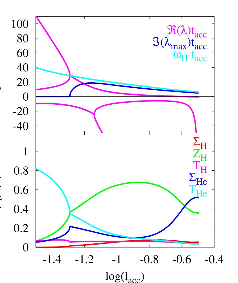
Figure 3.— Top panel: spectrum of the real parts of the eigenvalues as a function of $l_{\mathrm{acc}}$. Also shown are the imaginary part of the eigenvalue with the greatest real part and $\omega_{\mathrm{H}}\equiv 2\pi/t_{\mathrm{H}}$, where $t_{\mathrm{H}}\equiv\Sigma_{\mathrm{H}}^{\mathrm{eq}}/\dot{\Sigma}$ is the hydrogen-burning timescale. Each frequency is multiplied by the accretion timescale $t_{\mathrm{acc}}\equiv\Sigma_{\mathrm{He}}^{\mathrm{eq}}/\dot{\Sigma}$. Bottom panel: normalized components of the eigenvector corresponding to the eigenvalue with the greatest real part.

Figure 3 nicely illustrates the nature of the instability and the behavior of the resulting type I X-ray burst as a function of the accretion rate. For $\log(l_{\mathrm{acc}})\lesssim-1.3$, $\lambda$ is real and ${\bf v}$ is dominated by perturbations in $T_{\mathrm{He}}$, showing that a pure thermal perturbation in the helium burning region triggers the instability. Also, the perturbation grows very quickly since $\Re(\lambda)t_{\mathrm{acc}}\gg 1$. Hydrogen burning is clearly inconsequential to the instability since perturbations grow at a rate $\Re(\lambda)>\omega_{\mathrm{H}}$, where

$$\omega_{\mathrm{H}}\equiv\frac{2\pi}{t_{\mathrm{H}}}$$ (49)

and

$$t_{\mathrm{H}}\equiv\frac{\Sigma_{\mathrm{H}}^{\mathrm{eq}}}{\dot{\Sigma}}$$ (50)

is the hydrogen-burning timescale. These bursts (named helium bursts by NH03) are triggered by the well-known and standard thin-shell thermal instability.

For $-1.3\lesssim\log(l_{\mathrm{acc}})\lesssim-0.9$, $\Re(\lambda)t_{\mathrm{acc}}\gg 1$ so the bursts are still “prompt,” but now $\lambda$ is complex. This means that there is an overstability rather than a pure instability. Also, $\Re(\lambda)<\omega_{\mathrm{H}}$, which means that hydrogen burning now begins to play a role in the stability of the system. As a confirmation, we note that ${\bf v}$ involves perturbations of all five parameters, in particular the composition of the hydrogen-burning zone, showing that all the variables play a role in the instability.

For $-0.9\lesssim\log(l_{\mathrm{acc}})\lesssim-0.6$, $\Re(\lambda)t_{\mathrm{acc}}\lesssim 1$ and $\Im(\lambda)/\Re(\lambda)\gg 1$. This is the regime of delayed mixed bursts identified by NH03. The growing mode is overstable and undergoes several oscillations as the amplitude slowly increases. The angular frequency of the oscillations $\Im(\lambda)\approx\omega_{\mathrm{H}}$, showing that hydrogen burning plays a key role. We have verified that the imaginary parts of the eigenvalues in this regime derived using the global linear stability analysis of NH03 are approximately equal to $\omega_{\mathrm{H}}$ as well.

Finally, all eigenvalues have negative real parts for $\log(l_{\mathrm{acc}})\gtrsim-0.6$, and so no bursts occur at these high accretion rates. The $\Sigma_{\mathrm{He}}$ component begins to dominate ${\bf v}$ in this regime. For these systems, the effective radiative cooling rate of the accreted layer, which is proportional to $\Sigma_{\mathrm{He}}^{-2}$ (e.g., Fujimoto et al., 1981; Bildsten, 1998), is large enough to dampen any oscillations that might otherwise initiate an instability.

It is now clear why we are able to drop the terms $\propto\dot{\Sigma}$ in equation (2). In the helium and prompt mixed burst regimes, these terms are unimportant because thermal perturbations drive the instability, and they occur on a timescale much shorter than the accretion timescale $t_{\mathrm{acc}}$ (e.g., Bildsten, 1998). In the delayed mixed burst regime, although the mode grows on a timescale comparable to the accretion timescale, compositional perturbations primarily drive the overstability.

We consider our five-parameter, two-zone model to be “minimal,” by which we mean that no model consisting of only a proper subset of the five time-dependent variables $\Sigma_{\mathrm{H}}$, $Z_{\mathrm{H}}$, $T_{\mathrm{H}}$, $\Sigma_{\mathrm{He}}$, and $T_{\mathrm{He}}$ is able to reproduce the phenomenon of delayed mixed bursts. To demonstrate this, and to illustrate the specific role each parameter plays, we conduct linear stability analyses on truncated $n$-parameter models, where $n<5$, and we compare the results of these models to those of the full model. To perform these calculations, we determine the equilibria of the five parameters as usual, but we perturb only the $n$ parameters $\delta x_{i}$ and set the perturbations of the other $5-n$ parameters $\delta x_{i}=0$. We then solve for the eigenvalues of the corresponding $n\times n$ Jacobian matrix. See Figure 4 for plots of the real part of the largest eigenvalue of each model as a function of $l_{\mathrm{acc}}$. The middle dotted line is the eigenvalue for an isobaric purely thermal perturbation, where $\delta\Sigma_{\mathrm{H}}=\delta\Sigma_{\mathrm{He}}=\delta Z_{\mathrm{H}}=0$. All equilibria of this model are stable for $\log(l_{\mathrm{acc}})\gtrsim-1.2$. This result nicely complements the eigenvector analysis shown in Figure 3, which illustrates that thermal perturbations drive the instability for $\log(l_{\mathrm{acc}})\lesssim-1.2$, but they become less important for higher accretion rates. Using their global linear stability analysis, NH03 performed similar calculations in which they considered only thermal perturbations, and they obtained very similar results (see their Figures 16 and 17). The bottommost dotted line is the eigenvalue for a model in which only $\delta Z_{\mathrm{H}}=0$. This is a thermal perturbation as well, i.e., it includes no perturbation in the nuclear composition parameter $Z_{\mathrm{H}}$, but it is one in which the isobaric constraint is relaxed. Figure 4 shows again that all equilibria are stable for $\log(l_{\mathrm{acc}})\lesssim-1.2$. However, the eigenvalues near the transition between stability and instability are now complex. This is evident from the kink in the line at $\log(l_{\mathrm{acc}})\approx-1.35$, indicating that two real eigenvalues have merged into a complex-conjugate pair. The topmost dotted line is the eigenvalue for a model in which $\delta\Sigma_{\mathrm{H}}=\delta\Sigma_{\mathrm{He}}=0$. This perturbation is again isobaric, but it involves both thermal and compositional perturbations. Figure 4 shows that the eigenvalue is real, and that all equilibria are unstable.

Figure 4.— Real part of the largest eigenvalue as a function of $l_{\mathrm{acc}}$ for three models in which only a proper subset of the five parameters $\Sigma_{\mathrm{H}}$, $Z_{\mathrm{H}}$, $T_{\mathrm{H}}$, $\Sigma_{\mathrm{He}}$, and $T_{\mathrm{He}}$ is perturbed. The dotted lines show the normalized eigenvalues for models in which from top to bottom (i) $\delta\Sigma_{\mathrm{H}}=\delta\Sigma_{\mathrm{He}}=0$, (ii) $\delta\Sigma_{\mathrm{H}}=\delta\Sigma_{\mathrm{He}}=\delta Z_{\mathrm{H}}=0$, and (iii) $\delta Z_{\mathrm{H}}=0$. The solid line shows the normalized eigenvalue for the full model.

To better understand the role each parameter plays in the stability of the dynamical system, we first divide the perturbations into two classes. Equations (2) and (2) imply that $\delta T_{\mathrm{H}}$ and $\delta T_{\mathrm{He}}$ change on timescales on the order of the thermal diffusion timescale, whereas equations (31), (34), and (32) imply that $\delta\Sigma_{\mathrm{H}}$, $\delta\Sigma_{\mathrm{He}}$, and $\delta Z_{\mathrm{H}}$ change on timescales on the order of the accretion timescales $t_{\mathrm{H}}$ and $t_{\mathrm{acc}}$, which are usually much longer than the thermal diffusion timescale. Figures 3 and 4 demonstrate that, for $\log(l_{\mathrm{acc}})\lesssim-1.2$, purely thermal perturbations drive the instability, which grows on a timescale much shorter than the accretion timescale. A positive temperature perturbations $\delta T_{\mathrm{He}}>0$ grows quickly and accelerates helium burning, which decreases $\delta\Sigma_{\mathrm{He}}$. Although a decrease in $\delta\Sigma_{\mathrm{He}}$ increases the effective cooling rate, it does so over a much longer timescale, and so the effective cooling rate is usually unable to compensate for the positive temperature perturbation. Therefore, the system is still thermally unstable. Thus, for thermal perturbations, it makes little difference whether or not one allows $\delta\Sigma_{\mathrm{H}}$ and $\delta\Sigma_{\mathrm{He}}$ to vary with regard to the stability of the system (Paczyński, 1983a; Heger et al., 2005).

The situation is quite different for the delayed mixed burst regime, in which compositional perturbations $\delta Z_{\mathrm{H}}$ primarily drive the instability. A positive perturbation of any one of the three parameters $\delta T_{\mathrm{H}}$, $\delta T_{\mathrm{He}}$, or $\delta Z_{\mathrm{H}}$ will cause the other two to grow as well, for a positive temperature perturbation accelerates helium burning, which produces more CNO and hence increases $\delta Z_{\mathrm{H}}$, and a positive $\delta Z_{\mathrm{H}}$ perturbation accelerates hydrogen burning, which raises the temperature and hence increases $\delta T_{\mathrm{H}}$ and $\delta T_{\mathrm{He}}$. Since this system is stable to purely thermal perturbations, any unstable modes grow on the slow accretion timescale. But $\delta\Sigma_{\mathrm{H}}$ and $\delta\Sigma_{\mathrm{He}}$, which regulate the effective cooling rate, vary over a similar timescale. Therefore, $\delta\Sigma_{\mathrm{H}}$ and $\delta\Sigma_{\mathrm{He}}$ have time to respond to changes in the nuclear heating rate in this regime. A positive perturbation in any one of $\delta T_{\mathrm{H}}$, $\delta T_{\mathrm{He}}$, or $\delta Z_{\mathrm{H}}$ grows slowly and accelerates both hydrogen and helium burning, which decrease $\delta\Sigma_{\mathrm{H}}$ and $\delta\Sigma_{\mathrm{He}}$. Decreases in $\delta\Sigma_{\mathrm{H}}$ and $\delta\Sigma_{\mathrm{He}}$ raise the effective cooling rate over a similar timescale, which lowers the temperature and dampens nuclear burning. Consequently, $\delta\Sigma_{\mathrm{H}}$ and $\delta\Sigma_{\mathrm{He}}$ then slowly increase as freshly accreted matter advects into the layer until nuclear burning begins again. This cycle repeats, driving oscillations with a period on the order of the hydrogen burning timescale $t_{\mathrm{H}}$.

4. Time Evolution of the Onset of Delayed Mixed Bursts

Although linear stability analyses of the set of governing differential equations clearly determine whether or not the system will exhibit type I X-ray bursts, they can only hint at the nonlinear development of the instability and the underlying physics of the burst onset. To remedy this, we numerically integrate equations (31-2) to study the nonlinear evolution of the onset of delayed mixed bursts. We will not discuss the onset of prompt bursts in any detail, since the physics of prompt bursts has been previously studied by many authors and is generally well understood (Joss, 1978; Taam & Picklum, 1979; Joss & Li, 1980; Taam, 1980; Ayasli & Joss, 1982; Hanawa & Sugimoto, 1982; Taam, 1982; Paczyński, 1983b; Taam et al., 1993; Zingale et al., 2001; Woosley et al., 2004).

We perform the integration for a system with $\log(l_{\mathrm{acc}})=-0.7$, which is well inside the delayed mixed burst regime. Figure 3 shows that the system is marginally unstable, with $\Re(\lambda)t_{\mathrm{acc}}\approx 0.75$, and that the system undergoes oscillations with a period approximately equal to the hydrogen-burning timescale $t_{\mathrm{H}}$. We initiate the overstability by perturbing the equilibrium such that the initial conditions of the integration ${\bf x}_{0}=1.001\bf x^{\mathrm{eq}}$. Figure 5 shows the results of this calculation. The top panel illustrates the time evolution of the physical parameters. All modes other than the principal mode are transient and quickly decay after the initial perturbation. $T_{\mathrm{H}}$ and $T_{\mathrm{He}}$ are essentially in phase since the thermal diffusion timescale between $\Sigma_{\mathrm{H}}$ and $\Sigma_{\mathrm{He}}$ is much smaller than $t_{\mathrm{H}}$. The other physical parameters are pairwise out of phase, but each slowly grows and oscillates with the principal mode (Buchler, 1993). One can ascertain the relative phases by contrasting the phases of the various components of the complex eigenvector ${\bf v}$. For a comparison, we plot the time evolution of the physical parameters for a sequence of prompt bursts from a system with $\log(l_{\mathrm{acc}})=-1.4$ in Figure 6. The results of this prompt burst calculation are very similar to those of previous one- and two-zone models (Barranco et al., 1980; Paczyński, 1983a; Regev & Livio, 1984; Heger et al., 2005).

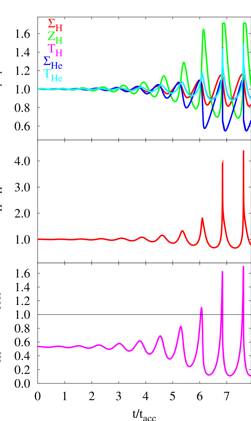
Figure 5.— Example of the time evolution of the overstability preceding a delayed mixed burst. $\xout{=}0.7$, $Z_{0}=0.02$, and $\log(l_{\mathrm{acc}})=-0.7$ for this calculation. Top panel: evolution of the normalized physical quantities. Middle panel: normalized lightcurve. Bottom panel: evolution of the ratio $(\partial\epsilon_{\mathrm{He}}/\partial T)/(\partial\epsilon_{\mathrm{cool}}/\partial T)$ evaluated at $\Sigma_{\mathrm{He}}$. A thin-shell thermonuclear instability ensues when $(\partial\epsilon_{\mathrm{He}}/\partial T)/(\partial\epsilon_{\mathrm{cool}}/\partial T)>1$.

Figure 6.— Example of the time evolution of prompt bursts. $\xout{=}0.7$, $Z_{0}=0.02$, and $\log(l_{\mathrm{acc}})=-1.4$ for this calculation. The top panel shows the lightcurve, and the bottom three panels show the time evolution of the five physical quantities. Note that $T_{\mathrm{He}}>T_{\mathrm{H}}$ and $\Sigma_{\mathrm{He}}>\Sigma_{\mathrm{H}}$.

To better understand the physics of the overstability preceding a delayed mixed burst, we consider a positive $T_{\mathrm{H}}$ perturbation. Since the thermal diffusion time from $\Sigma_{\mathrm{H}}$ to $\Sigma_{\mathrm{He}}$ is very short, $T_{\mathrm{He}}$ follows the time dependence of $T_{\mathrm{H}}$ throughout the integration. An increase in $T_{\mathrm{H}}$ causes the helium in zone (i) to burn at a higher rate, which increases $Z_{\mathrm{H}}$, and the simultaneous increase in $T_{\mathrm{He}}$ causes the helium in zone (ii) to burn at a higher rate also, which decreases $\Sigma_{\mathrm{He}}$. The larger $Z_{\mathrm{H}}$ causes hydrogen to burn at a higher rate, which decreases $\Sigma_{\mathrm{H}}$. This raises the effective cooling rate of the accreted layer, which is proportional to $1/\Sigma_{\mathrm{H}}^{2}$. When nuclear burning has nearly depleted the hydrogen in zone (i), both of the zones cool as freshly accreted matter advects down to larger column depths. $T_{\mathrm{H}}$ and $T_{\mathrm{He}}$ consequently decrease until enough nuclear fuel has accumulated to restart nuclear burning. Once this happens, $T_{\mathrm{H}}$ and $T_{\mathrm{He}}$ will increase and the cycle continues.

If the amplitudes of the oscillations increase in time, the temperature $T_{\mathrm{He}}$ at $\Sigma_{\mathrm{He}}$ may raise the helium nuclear energy generation rate high enough to trigger a thin-shell thermal instability and hence a type I X-ray burst. To understand when the burst will occur, we follow the basic one-zone, single-parameter linear stability analysis of Fujimoto et al. (1981) and consider the effective radiative cooling rate at $\Sigma_{\mathrm{He}}$

$$\epsilon_{\mathrm{cool}}\equiv\frac{acT_{\mathrm{He}}^{4}}{3\kappa\Sigma_{\mathrm{He}}^{2}}.$$ (51)

A thin-shell thermal instability develops when

$$\frac{\partial\epsilon_{\mathrm{He}}}{\partial T}>\frac{\partial\epsilon_{\mathrm{cool}}}{\partial T}$$ (52)

(Fujimoto et al., 1981; Hanawa & Fujimoto, 1982; Fushiki & Lamb, 1987). We plot the ratio $(\partial\epsilon_{\mathrm{He}}/\partial T)/(\partial\epsilon_{\mathrm{cool}}/\partial T)$ in the bottom panel of Figure 5. A comparison between the lightcurve shown in the middle panel and the ratio $(\partial\epsilon_{\mathrm{He}}/\partial T)/(\partial\epsilon_{\mathrm{cool}}/\partial T)$ in the bottom panel shows that a short type I X-ray burst, characterized by a sudden increase in the outward flux, occurs when the thin-shell thermal instability criterion $(\partial\epsilon_{\mathrm{He}}/\partial T)/(\partial\epsilon_{\mathrm{cool}}/\partial T)>1$ is satisfied. Note that the low peak flux of the burst is due to the restriction in our model that hydrogen burns only via the temperature-independent hot CNO cycle. In our two-zone model, this delayed mixed burst calculation evolves to a limit cycle of short bursts with a recurrence time $\approx t_{\mathrm{H}}$. In reality, hydrogen burning will proceed via the rp-process of Wallace & Woosley (1981) during the burst, and this will burn nearly all of the fuel and produce an Eddington-limited flux (e.g., Hanawa & Fujimoto, 1984; Woosley et al., 2004; Fisker et al., 2006). The system will then restart near $t/t_{\mathrm{acc}}\approx 0$ in Figure 5 and undergo several oscillations before having its next burst. Our two-zone model, which includes no rp-process reactions, is too simple to reproduce this behavior. Note also that, while equation (51) is the exact cooling rate for a suitably constructed one-zone model, it is only approximate for our two-zone model. However, it is accurate enough to illustrate that, much like prompt bursts, helium burning ultimately induces a thin-shell thermal instability that triggers a delayed mixed burst.

While the above calculation illustrates the physics of the onset of delayed mixed bursts, it does not unambiguously demonstrate that the bursts are in fact “delayed.” Specifically, we have not yet demonstrated that a significant period of stable burning will precede a type I X-ray burst. Although we began the integration by perturbing the equilibrium solution, a system that is dynamically unstable need not come anywhere close to its equilibrium. Unfortunately, we cannot set the initial conditions to that of a bare neutron star, for which ${\bf x_{0}}=$ {$\Sigma_{\mathrm{H}},Z_{\mathrm{H}},T_{\mathrm{H}},\Sigma_{\mathrm{He}},T_{\mathrm{He}}$} = {$0,Z_{0},0,0,0$}, because the time steps required to begin the integration from these initial conditions are too small to maintain numerical accuracy. Instead, we set ${\bf x_{0}}=$ {$\Sigma_{\mathrm{H}}^{\mathrm{eq}},Z_{\mathrm{H}}^{\mathrm{eq}},T_{\mathrm{H}}^{\mathrm{eq}},\Sigma_{\mathrm{H}}^{\mathrm{eq}}$, $T_{\mathrm{H}}^{\mathrm{eq}}$}, i.e. we start the system with the hydrogen-burning layer in place but without any helium-burning layer. We then integrate until a type I X-ray burst occurs. This calculation gives a recurrence time $t_{\mathrm{rec}}\equiv t_{\mathrm{H}}+t_{\mathrm{int}}$, where $t_{\mathrm{int}}$ is the integration time. From the recurrence time, we derive an estimate for the dimensionless quantity $\alpha$, which is defined as the accretion energy released between successive bursts divided by the nuclear energy released during a burst. Thus,

$$\alpha\approx\frac{\dot{\Sigma}c^{2}zt_{\mathrm{rec}}}{[\xout{E^{*}_{\mathrm{H}}}+(1-Z_{0})E^{*}_{\mathrm{He}}]\Sigma_{\mathrm{H}}+(1-Z_{\mathrm{H}})E^{*}_{\mathrm{He}}\Sigma_{\mathrm{He}}},$$ (53)

where $z=(1-2GM/Rc^{2})^{-1/2}-1$ is the gravitational redshift, and the values of $\Sigma_{\mathrm{H}}$, $Z_{\mathrm{H}}$, and $\Sigma_{\mathrm{He}}$ are determined from the numerical integration just prior to the burst. Both the accretion energy and nuclear energy of the burst in equation (53) are those measured locally at the stellar surface. In our expression for $\alpha$, we implicitly assume that all of the hydrogen and helium burns to CNO during a burst. Figure 7 shows that $\alpha\sim 100$ in the regime of prompt bursts, which is consistent with more sophisticated calculations (e.g., Woosley et al., 2004), and that $\alpha$ rises dramatically to values $\sim 1000$ for $\log(l_{\mathrm{acc}})\gtrsim-0.9$, which illustrates that the systems in the delayed mixed burst regime undergo long periods of stable nuclear burning prior to type I X-ray bursts. This is consistent with both the results of NH03 (see their Figures 15 and 18) and observations (van Paradijs et al., 1988).

Figure 7.— Shows $\alpha$-values of type I X-ray bursts as a function of $l_{\mathrm{acc}}$. The steep rise in $\alpha$ beginning at $\log(l_{\mathrm{acc}})\approx-0.9$ as $l_{\mathrm{acc}}$ increases is characteristic of delayed mixed bursts.

5. Discussion

In this section, we compare and contrast the results of the two-zone model presented in this work with the results of both the global linear stability analysis of NH03 and other theoretical models.

5.1. Comparison to the Global Stability Analysis of Narayan & Heyl

The primary goal of this work is to construct a simple model of nuclear burning on accreting neutron stars that elucidates the essential physics behind the more complicated and abstruse global linear stability analysis of NH03. We assess how well we have accomplished this goal below.

We begin by discussing the various bursting regimes and the ranges of accretion rates $l_{\mathrm{acc}}$ in which these regimes lie. A comparison between the results of §3 and Table 3 of NH03 demonstrates that the two-zone model reproduces all of the bursting regimes of NH03 for the relatively high $l_{\mathrm{acc}}$ considered in this work, and that the ranges of $l_{\mathrm{acc}}$ coincide very well with the results of NH03’s “canonical” neutron star, for which $M=1.4M_{\odot}$, $R=10.4$ km, and $T_{\mathrm{core}}=10^{8}$ K . However, the two-zone model cannot reproduce the hydrogen bursts that occur for $\log(l_{\mathrm{acc}})\lesssim-2.5$ because unstable thermonuclear hydrogen burning triggers these burst, but our expression for $\epsilon_{\mathrm{H}}$ is temperature-independent. We note that the $l_{\mathrm{acc}}$ ranges of the various regimes in the two-zone model depend somewhat on the values of $\kappa$ and $\gamma_{\mathrm{He}}$, assumed constant in our model.

The methods used to determine the equilibrium solution in each model differ somewhat, although this difference should not affect the eigenvalue. NH03 started with an assumed column depth of accreted plasma $\Sigma_{\mathrm{layer}}$ and determined the equilibrium solution of the physical quantities $\rho$, $T$, $F$, $X$, and $Y$ as functions of $\Sigma$. Next, they carried out a linear perturbation analysis to determine the stability of the equilibrium solution. If $\Re(\lambda)t_{\mathrm{acc}}\geq 3$, where in this case $t_{\mathrm{acc}}\equiv\Sigma_{\mathrm{layer}}/\dot{\Sigma}$, then the configuration was unstable and a type I X-ray burst was assumed to occur. If $\Re(\lambda)t_{\mathrm{acc}}<3$, the configuration was stable, and the process was repeated for a larger value of $\Sigma_{\mathrm{layer}}$. If $\Re(\lambda)t_{\mathrm{acc}}<3$ for all trial values of $\Sigma_{\mathrm{layer}}$, then the system was stable, and no type I X-ray bursts occurred. It is important to understand that the method of NH03 will find all systems that have positive eigenvalues to be unstable because $t_{\mathrm{acc}}$ increases as $\Sigma_{\mathrm{layer}}$ increases. In the two-zone model, we assume complete burning of the accreted matter, and we say that type I X-ray bursts occur if $\Re(\lambda)t_{\mathrm{acc}}>0$ and that no bursts occur otherwise. If a system is stable to bursts, the accreted matter steadily burns to completion, and both methods agree that this equilibrium is stable. If a system is unstable to bursts, the two-zone model determines that the complete steady-burning equilibrium solution is unstable. The method of NH03 may find that the identical system is unstable either before all of the fuel burns to completion (in a prompt burst, for example) or after all the fuel burns to completion (in, say, a delayed burst), but it will always determine that the system is indeed unstable. Therefore, although the two stability analyses differ to some extent, these differences are unimportant with respect to the determination of the eigenvalue of a system.

The eigenvalues derived using the two models agree quite well. We have shown already that the real parts of the eigenvalues agree quite well, for they delineate between the prompt and delayed bursting regimes. We now compare the imaginary parts. We have shown in §3 that $\Im(\lambda)\approx\omega_{\mathrm{H}}$ in the delayed mixed burst regime, which means that oscillations occur with a period equal to the hydrogen-burning timescale. To explicitly show that $\Im(\lambda)\approx\omega_{\mathrm{H}}$ in the global linear stability analysis, we consider the calculation presented in §4.2 of NH03. In that calculation, NH03 consider a system with $\log(l_{\mathrm{acc}})=-0.9$, which implies that $\dot{\Sigma}=1.04\times 10^{4}$ $\mathrm{g}\,\mathrm{cm}^{-2}\,\mathrm{s}^{-1}$, since $\dot{\Sigma}_{\mathrm{Edd}}=8.26\times 10^{4}$ $\mathrm{g}\,\mathrm{cm}^{-2}\,\mathrm{s}^{-1}$ for that system. Figures 8 and 9 of NH03 imply that $\Sigma_{\mathrm{H}}^{\mathrm{eq}}\approx 1.0\times 10^{8}$ $\mathrm{g}\,\mathrm{cm}^{-2}$, and so $\omega_{\mathrm{H}}=6.5\times 10^{-4}$ $\mathrm{s}^{-1}$ from equations (49) and (50). This value of $\omega_{\mathrm{H}}$ is very close to the $6.6\times 10^{-4}$ $\mathrm{s}^{-1}$ NH03 quote for the imaginary part of the eigenvalue they obtained in their calculation.

Revnivtsev et al. (2001) discovered a class of low-frequency oscillations that precede type I X-ray bursts in the systems 4U 1608$-$522, 4U 1636$-$536, and Aql X-1. These oscillations have periods $\sim 120$ seconds and have been observed when the accretion rate $l_{\mathrm{acc}}\approx 0.1$. While the modes resulting from the global stability analysis of NH03 are complex in this regime, the oscillation periods of these modes are roughly a factor of $10$ larger than the observed periods. It is now clear why NH03 were unsuccessful in explaining these observations. We have shown in §3 that the oscillation periods of overstable modes in this regime are approximately equal to the hydrogen-burning timescale $t_{\mathrm{H}}$. From equations (39) and (50),

$$t_{\mathrm{H}}=\frac{2\xout{missing}}{\gamma_{\mathrm{H}}(Z_{\mathrm{H}}^{\mathrm{eq}}+Z_{0})}>770\left(\frac{\xout{missing}}{0.7}\right)\mathrm{s}.$$ (54)

Thus the oscillations preceding a delayed mixed burst have too long of a period and cannot be associated with the oscillations observed by Revnivtsev et al. (2001) if hydrogen burns predominantly via the hot CNO cycle.

We have shown in §4 that, in the delayed mixed burst regime, a considerable amount of stable burning occurs prior to a type I X-ray burst. Consequently, $\alpha$, the ratio of the gravitational energy released via accretion to the nuclear energy released during a burst, rises dramatically near the critical $l_{\mathrm{acc}}$ above which bursts do not occur. A comparison between Figure 7 of this work and Figure 15 of NH03 demonstrates that the $\alpha$-values derived using the two different models agree quite well.

Using an improved version of the model of NH03, Cooper et al. (2006) found that increasing $Z_{0}$, the CNO abundance of the accreted plasma, diminishes the range of $l_{\mathrm{acc}}$ over which delayed mixed bursts occur. In fact, for large enough values of $Z_{0}$, Cooper et al. (2006) found that the ranges of $l_{\mathrm{acc}}$ in which prompt mixed bursts and delayed mixed bursts occur are separated by a regime of stable burning. Figure 8$a$ shows the normalized eigenvalues of the two-zone model for systems in which $Z_{0}\geq 0.02$. The critical $l_{\mathrm{acc}}$ above which bursts do not occur decreases with increasing $Z_{0}$, in agreement with Figure 5 of Cooper et al. (2006), but the two-zone model does not reproduce the regime of stable burning that separates the prompt mixed bursts from the delayed mixed bursts for our choices of $\kappa$ and $\gamma_{\mathrm{He}}$. However, we are able to reproduce this regime with certain combinations of $Z_{0}$, $\kappa$, and $\gamma_{\mathrm{He}}$. Figure 8$b$ shows the normalized eigenvalues for a model in which $Z_{0}=0.132$ and $\gamma_{\mathrm{He}}=0.3$. A stable burning regime separating prompt mixed bursts from the delayed mixed bursts is clearly evident for this calculation, showing that the two-zone model has the right qualitative behavior. However, our choice of $Z_{0}$ for this calculation is more than twice that required in the more accurate model of Cooper et al. (2006), showing that (not surprisingly) there are quantitative discrepancies.

Figure 8.— Real part of the largest eigenvalue as a function of $l_{\mathrm{acc}}$. ($a$) Normalized eigenvalue for models in which from top to bottom $Z_{0}=0.02$, $0.04$, $0.06$, $0.08$, $0.10$, and $0.12$. ($b$) Normalized eigenvalue for a model in which $Z_{0}=0.132$ and $\gamma_{\mathrm{He}}=0.3$. The prompt mixed burst and delayed mixed burst regimes are clearly separated by a regime of stable nuclear burning.

5.2. Comparison to Previous Theoretical Work

For accretion rates $l_{\mathrm{acc}}\lesssim 0.1$, type I X-ray bursts are well-understood theoretically, and the results of theoretical models are generally in accord with observations. This is not true for $l_{\mathrm{acc}}\gtrsim 0.1$. Nearly all theoretical models predict that accreting neutron stars should exhibit type I X-ray bursts for all $l_{\mathrm{acc}}\lesssim 1$ (Fujimoto et al., 1981; Ayasli & Joss, 1982; Taam, 1985; Taam et al., 1996; Bildsten, 1998; Fisker et al., 2003; Heger et al., 2005), whereas the model of NH03 and the two-zone model presented in this work suggest that bursts should cease for $l_{\mathrm{acc}}\gtrsim 0.25$, in agreement with observations (van Paradijs et al., 1979, 1988; Cornelisse et al., 2003; Remillard et al., 2006). Furthermore, our model and that of NH03 are the only models able to explain the dramatic increase in $\alpha$ with increasing $l_{\mathrm{acc}}$ observed by van Paradijs et al. (1988). In this section, we compare and contrast the two-zone model presented in this work with previous one-zone burst models. Additionally, we discuss the results of this work in relation to those of detailed time-dependent multi-zone models that utilize sophisticated nuclear reaction networks.

We begin by discussing the stability criterion of one-zone models (e.g., Fujimoto et al., 1981; Paczyński, 1983a; Bildsten, 1998; Cumming & Bildsten, 2000; Heger et al., 2005). These models presume that helium burning (or hydrogen burning for very low $l_{\mathrm{acc}}$) initiates a thermonuclear instability and produces a type I X-ray burst. As mentioned in §2, the hydrogen burning rate is temperature-independent for $T\gtrsim 10^{8}$ K and so hydrogen burning cannot be thermally unstable for $l_{\mathrm{acc}}\gtrsim 0.01$. Since all of the one-zone models give very similar results, we focus on the model of Heger et al. (2005), which is an extension of the model of Paczyński (1983a), for a comparison. Written in our notation, the differential equations (1-2) of Heger et al. (2005) that govern their model are

$$\frac{d\Sigma_{\mathrm{He}}}{dt}=\dot{\Sigma}-\Sigma_{\mathrm{He}}\frac{\epsilon_{\mathrm{He}}(T_{\mathrm{He}})}{E^{*}_{\mathrm{He}}},$$ (55)

$$\frac{dT_{\mathrm{He}}}{dt}=\frac{1}{C_{\mathrm{p}}}\left[\epsilon_{\mathrm{He}}(T_{\mathrm{He}})-\frac{F_{\mathrm{He}}}{\Sigma_{\mathrm{He}}}\right],$$ (56)

where $F_{\mathrm{He}}=acT_{\mathrm{He}}^{4}/3\kappa\Sigma_{\mathrm{He}}$. They presume that $\Sigma_{\mathrm{H}}^{\mathrm{eq}}>\Sigma_{\mathrm{He}}^{\mathrm{eq}}$ and that no stable helium burning occurs prior to the burst. The equilibrium solution to equations (55-56) is

$$\epsilon_{\mathrm{He}}(T_{\mathrm{He}})\Sigma_{\mathrm{He}}=F_{\mathrm{He}}=\dot{\Sigma}E^{*}_{\mathrm{He}},$$ (57)

or equivalently,

$$\epsilon_{\mathrm{He}}(T_{\mathrm{He}})=\epsilon_{\mathrm{cool}},$$ (58)

where $\epsilon_{\mathrm{cool}}$ is given by equation (51). Using the thin-shell thermal instability criterion of equation (52), one finds that the transition from stability to instability occurs when $\nu\equiv\partial\ln\epsilon_{\mathrm{He}}/\partial\ln T\approx 4$, since $\partial\ln\epsilon_{\mathrm{cool}}/\partial\ln T=4$. One finds nearly the same condition by performing a standard linear stability analysis on equations (55) and (56). Thus, from equation (15), the equilibria are stable to bursts when $T_{\mathrm{He}}^{\mathrm{eq}}\gtrsim 6\times 10^{8}$ K. However, Figures 2 and 4 illustrate that many of the equilibria in our two-zone model are stable to thermal perturbations for temperatures much less than $6\times 10^{8}$ K. To understand this, note that equation (58) implies that helium burning is the only source of nuclear energy generation. In our two-zone model, both hydrogen burning and helium burning are sources of nuclear energy generation, and so qualitatively $\epsilon_{\mathrm{cool}}\sim\epsilon_{\mathrm{He}}(T)+\epsilon_{\mathrm{H}}(Z)$. Hydrogen burning is temperature-independent, so equation (52) still gives the right criterion for a thin-shell thermal instability. However, because $\epsilon_{\mathrm{cool}}>\epsilon_{\mathrm{He}}$, the critical value of $\nu$ for instability is larger than $4$. Roughly, on expects something like $\nu_{\mathrm{crit}}\sim 4(\epsilon_{\mathrm{cool}}/\epsilon_{\mathrm{He}})$. Several authors (e.g., Fujimoto et al., 1981; Cumming & Bildsten, 2000) have included the effect of hydrogen burning on the stability criterion in their one-zone models. These models assume that no helium burning takes place prior to ignition, so $Z=Z_{0}$ throughout the accreted layer. Consequently, they find that the effect of hydrogen burning on the stability of the system is minor. In contrast, stable helium burning prior to ignition is substantial for $l_{\mathrm{acc}}\gtrsim 0.1$ in both our two-zone model and that of NH03, and so the effect of hydrogen burning on the stability of the system is considerable. Thus, hydrogen burning via the temperature-independent hot CNO cycle, augmented by the extra CNO produced from stable helium burning, helps stabilize nuclear burning on accreting neutron stars even at temperatures $\sim 3\times 10^{8}$ K, which is much less than the $\sim 6\times 10^{8}$ K needed to stabilize pure helium burning.

In the limit $\xout{\rightarrow}0$ and $Z_{0}\rightarrow 0$, equations (31-2) of our two-zone model reduce to the following set of two coupled differential equations:

$$\frac{d\Sigma_{\mathrm{He}}}{dt}=2\left[\dot{\Sigma}-\Sigma_{\mathrm{He}}\frac{\epsilon_{\mathrm{He}}(T_{\mathrm{He}})}{E^{*}_{\mathrm{He}}}\right],$$ (59)

$$\frac{dT_{\mathrm{He}}}{dt}=\frac{5}{4C_{\mathrm{p}}}\left[\epsilon_{\mathrm{He}}(T_{\mathrm{He}})-\frac{F_{\mathrm{He}}}{\Sigma_{\mathrm{He}}}\right]+\frac{T_{\mathrm{He}}}{4\Sigma_{\mathrm{He}}}\frac{d\Sigma_{\mathrm{He}}}{dt},$$ (60)

where again $F_{\mathrm{He}}=acT_{\mathrm{He}}^{4}/3\kappa\Sigma_{\mathrm{He}}$ from equation (14), and the equilibrium is given by equation (57). Equations (59) and (60) are effectively the same as equations (55) and (56). With the system of equations (59-60), we are able to reproduce the results of the one-zone models of Paczyński (1983a) and Heger et al. (2005). As expected, the critical temperature for stability is $\sim 6\times 10^{8}$ K in this case.

It is perhaps not surprising that one-zone models that focus only on helium burning are not able to reproduce all of the bursting regimes found using global linear stability analyses or observed in nature. As we have shown in this paper, one needs at least two zones, one in which only helium burns and another in which both hydrogen and helium burn together, to incorporate all of the key physics included in the model of NH03. One-zone models simply do not include enough physics. More troubling is the fact that the results of detailed multi-zone calculations of type I X-ray bursts (e.g., Ayasli & Joss, 1982; Taam et al., 1996; Fisker et al., 2003; Heger et al., 2005) do not reproduce the regime of delayed mixed bursts and are also inconsistent with observations for $l_{\mathrm{acc}}\gtrsim 0.1$. Since we do not have access to such models, we are unable to conduct a direct comparison between our model and these numerical calculations. However, we attempt to better understand this discrepancy by considering the work of Fisker et al. (2006).

Fisker et al. (2006) study the effects of the relatively unconstrained ¹⁵O($\alpha$,$\gamma$)¹⁹Ne reaction rate on type I X-ray bursts from neutron stars accreting at $l_{\mathrm{acc}}\approx 0.1$. This reaction is one of the two hot CNO cycle breakout reactions (Wagoner, 1969; Wallace & Woosley, 1981; Langanke et al., 1986; Wiescher et al., 1999; Schatz et al., 1999). For the lowest of the three trial reaction rates they consider, they find that, after an initial type I X-ray burst, hydrogen and helium burn stably via the hot CNO cycle and triple-$\alpha$ reactions, respectively, and the nuclear burning generates a slowly oscillating luminosity with a period approximately equal to the hydrogen-burning timescale. The nuclear burning behavior in this calculation is nearly identical to that of the nuclear burning preceding a delayed mixed burst found in §4. This similarity is perhaps to be expected, for the limited reaction networks employed in the model of NH03 and the present model omit hot CNO cycle breakout reactions entirely. For the two higher trial reaction rates investigated by Fisker et al. (2006), the breakout sequence ¹⁵O($\alpha$,$\gamma$)¹⁹Ne($p$,$\gamma$)²⁰Na diminishes the CNO abundance and thus reduces the rate of hydrogen burning. Hence, when helium ignition commences, the helium energy generation rate dominates the total nuclear energy generation rate, and a prompt type I X-ray burst occurs via a thin-shell thermal instability. We tentatively suggest that the discrepancies between the results of the global linear stability analysis of NH03 and the results of multi-zone calculations arise from differences in the treatment of hot CNO cycle breakout reactions. In the NH03 model and our two-zone model, hydrogen burning via the temperature-independent hot CNO cycle helps stabilize nuclear burning on accreting neutron stars. Breakout reactions would reduce the degree to which hydrogen burns via the hot CNO cycle and thereby increase the temperature-sensitivity of the total effective nuclear energy generation rate. Thus, breakout reactions would presumably extend the range of accretion rates in which nuclear burning is thermally unstable, but we do not include these reactions. That observations agree much better with the results of NH03 and our two-zone model may imply that the true cross sections of reactions such as the hot CNO cycle breakout reactions ¹⁵O($\alpha$,$\gamma$)¹⁹Ne and ¹⁸Ne($\alpha$,$p$)²¹Na are much smaller than the cross sections employed in the reaction networks of multi-zone models, i.e., the true ¹⁵O($\alpha$,$\gamma$)¹⁹Ne reaction rate is closer to the lowest reaction rate considered by Fisker et al. (2006). By omitting hot CNO cycle breakout reactions altogether, the model of NH03 is perhaps a better representation of the nuclear burning that precedes type I X-ray bursts than time-dependent multi-zone models as presently implemented.

The model we present in §2 is valid only when $\Sigma_{\mathrm{H}}<\Sigma_{\mathrm{He}}$, which restricts the range of accretion rates we can study to $l_{\mathrm{acc}}\lesssim 0.3$. We have constructed a similar model to determine the stability of nuclear burning on accreting neutron stars for which $\Sigma_{\mathrm{H}}>\Sigma_{\mathrm{He}}$, allowing us to study the stability of nuclear burning at higher $l_{\mathrm{acc}}$. Although we find that all equilibria for $l_{\mathrm{acc}}\gtrsim 0.3$ are stable, which is consistent with the results of NH03, we cannot state with confidence that either the two-zone model or the model of NH03 is an accurate representation of nuclear burning on accreting neutron stars for such high accretion rates. For $l_{\mathrm{acc}}\gtrsim 1$, nuclear reactions other than the hot CNO cycle and triple-$\alpha$ reaction almost certainly play a significant role in the nuclear burning prior to a type I X-ray burst. It is possible that there exists another unstable burning regime near $l_{\mathrm{acc}}\sim 1$, and the range of $l_{\mathrm{acc}}$ in which this regime might exist would probably depend upon the $l_{\mathrm{acc}}$ at which the effective hydrogen-burning rate becomes predominantly temperature-dependent rather than composition-dependent. While most low-mass X-ray binaries with $l_{\mathrm{acc}}\gtrsim 0.3$ do not have type I X-ray bursts, GX 17+2 and Cyg X-2 are notable exceptions (Kahn & Grindlay, 1984; Tawara et al., 1984; Sztajno et al., 1986; Kuulkers et al., 1995, 1997; Wijnands et al., 1997; Smale, 1998; Kuulkers et al., 2002), although these sources may exhibit type I X-ray bursts for other reasons. For example, bursts could occur at $l_{\mathrm{acc}}\sim 1$ if the accreted plasma is hydrogen-deficient (e.g., Cooper et al., 2006).

6. Conclusions

We have constructed a simple two-zone model of type I X-ray bursts on accreting neutron stars. This model reproduces the delayed mixed burst regime of NH03 as well as the helium and prompt mixed burst regimes of previous studies (Fujimoto et al. 1981; Fushiki & Lamb 1987; Cumming & Bildsten 2000; NH03), and it agrees well with observations of type I X-ray bursts (van Paradijs et al., 1979, 1988; Cornelisse et al., 2003; Remillard et al., 2006). More importantly, the model illustrates the physics of the onset of instability as a function of the local accretion rate $\dot{\Sigma}$, and it facilitates comparisons between global linear stability analyses (which are more accurate but difficult to understand physically) and other burst models.

A pure, rapidly growing thermal instability in the helium-burning zone triggers bursts at relatively low $\dot{\Sigma}$. As $\dot{\Sigma}$ increases above $0.1\dot{\Sigma}_{\mathrm{Edd}}$, the trigger mechanism evolves from that of a thermal instability to that of a slowly growing overstability involving all parameters, particularly the CNO mass fraction $Z_{\mathrm{H}}$ of the hydrogen-burning zone. The competition between nuclear heating via the $\beta$-limited CNO cycle as well as the triple-$\alpha$ process and radiative cooling via outward diffusion of photons coupled with radiation from the stellar surface drives oscillations with a period approximately equal to the hydrogen-burning timescale $\Sigma_{\mathrm{H}}^{\mathrm{eq}}/\dot{\Sigma}$. If these oscillations grow in time, the temperature $T_{\mathrm{He}}$ at the base of the helium layer will rise, eventually triggering a thin-shell thermal instability and hence a delayed mixed burst. For $\dot{\Sigma}/\dot{\Sigma}_{\mathrm{Edd}}\gtrsim 0.25$ radiative cooling from the stellar surface dampens the overstability, and no bursts occur. We consider our two-zone model to be “minimal,” by which we mean that no model consisting of only a proper subset of the five time-dependent variables $\Sigma_{\mathrm{H}}$, $Z_{\mathrm{H}}$, $T_{\mathrm{H}}$, $\Sigma_{\mathrm{He}}$, and $T_{\mathrm{He}}$ is able to reproduce the phenomenon of delayed mixed bursts.

Nearly all other theoretical models predict that bursts should occur for all $\dot{\Sigma}/\dot{\Sigma}_{\mathrm{Edd}}\lesssim 1$, in disagreement with the results of both NH03 and the two-zone model, as well as with observations. We suggest that this discrepancy arises from the assumed strength of the hot CNO cycle breakout reaction ¹⁵O($\alpha$,$\gamma$)¹⁹Ne (Wagoner, 1969; Wallace & Woosley, 1981; Schatz et al., 1999; Fisker et al., 2006) in time-dependent multi-zone burst models. That observations agree much better with the results of both NH03 and this work may imply that the true ¹⁵O($\alpha$,$\gamma$)¹⁹Ne cross section is much smaller than the cross sections employed in the reaction networks of these models. Further calculations such as those presented by Fisker et al. (2006) in which the ¹⁵O($\alpha$,$\gamma$)¹⁹Ne reaction rate in the networks of time-dependent multi-zone models is varied should be performed.

We have considered only two forms of nuclear burning in our model: hydrogen burning via the hot CNO cycle and helium burning via the triple-$\alpha$ process. While this simplification is almost surely reasonable for studying the onset of helium bursts, certain additional reactions may be important in the delayed mixed burst regime or at yet higher $\dot{\Sigma}$. In particular, hot CNO cycle breakout reactions such as ¹⁵O($\alpha$,$\gamma$)¹⁹Ne could significantly affect the CNO metallicity $Z_{\mathrm{H}}$ of the hydrogen burning zone and consequently have some effect on delayed mixed bursts. Additional hydrogen burning processes that could circumvent the hot CNO cycle such as the ¹⁵O($p$,$\gamma$)($\beta^{+}\nu$)¹⁶O($p$,$\gamma$)¹⁷F($p$,$\gamma$)¹⁸Ne($\beta^{+}\nu$)¹⁸F($p$,$\alpha$)¹⁵O reaction sequence (Stefan et al., 2006) could affect delayed mixed bursts as well. These issues are worthy of further investigation.

References

- Ayasli & Joss (1982) Ayasli, S. & Joss, P. C. 1982, ApJ, 256, 637
- Babushkina et al. (1975) Babushkina, O. P., Bratolyubova-Tsulukidze, L. S., Kudryavtsev, M. I., Melioranskiy, A. S., Savenko, I. A., & Yushkov, B. Y. 1975, Soviet Astronomy Letters, 1, 32
- Barranco et al. (1980) Barranco, M., Buchler, J. R., & Livio, M. 1980, ApJ, 242, 1226
- Belian et al. (1976) Belian, R. D., Conner, J. P., & Evans, W. D. 1976, ApJ, 206, L135
- Bildsten (1998) Bildsten, L. 1998, in NATO ASIC Proc. 515: The Many Faces of Neutron Stars., 419
- Buchler (1993) Buchler, J. R. 1993, Ap&SS, 210, 9
- Buchler & Perdang (1979) Buchler, J. R. & Perdang, J. 1979, ApJ, 231, 524
- Cooper et al. (2006) Cooper, R. L., Mukhopadhyay, B., Steeghs, D., & Narayan, R. 2006, ApJ, 642, 443
- Cooper & Narayan (2005) Cooper, R. L. & Narayan, R. 2005, ApJ, 629, 422
- Cornelisse et al. (2003) Cornelisse, R., in’t Zand, J. J. M., Verbunt, F., Kuulkers, E., Heise, J., den Hartog, P. R., Cocchi, M., Natalucci, L., Bazzano, A., & Ubertini, P. 2003, A&A, 405, 1033
- Cumming (2004) Cumming, A. 2004, Nuclear Physics B Proceedings Supplements, 132, 435
- Cumming (2005) —. 2005, Nuclear Physics A, 758, 439
- Cumming & Bildsten (2000) Cumming, A. & Bildsten, L. 2000, ApJ, 544, 453
- Fisker et al. (2005) Fisker, J. L., Brown, E. F., Liebendörfer, M., Thielemann, F.-K., & Wiescher, M. 2005, Nuclear Physics A, 752, 604
- Fisker et al. (2006) Fisker, J. L., Gorres, J., Wiescher, M., & Davids, B. 2006, accepted by ApJ (astro-ph/0410561)
- Fisker et al. (2003) Fisker, J. L., Hix, W. R., Liebendörfer, M., & Thielemann, F.-K. 2003, Nuclear Physics A, 718, 614
- Fujimoto et al. (1981) Fujimoto, M. Y., Hanawa, T., & Miyaji, S. 1981, ApJ, 247, 267
- Fushiki & Lamb (1987) Fushiki, I. & Lamb, D. Q. 1987, ApJ, 323, L55
- Grindlay et al. (1976) Grindlay, J., Gursky, H., Schnopper, H., Parsignault, D. R., Heise, J., Brinkman, A. C., & Schrijver, J. 1976, ApJ, 205, L127
- Grindlay & Heise (1975) Grindlay, J. & Heise, J. 1975, IAU Circ., 2879
- Guckenheimer & Holmes (1983) Guckenheimer, J. & Holmes, P. 1983, Nonlinear Oscillations, Dynamical Systems, and Bifurcations of Vector Fields (Applied Mathematical Sciences, New York: Springer)
- Hanawa & Fujimoto (1982) Hanawa, T. & Fujimoto, M. Y. 1982, PASJ, 34, 495
- Hanawa & Fujimoto (1984) Hanawa, T. & Fujimoto, M. Y. 1984, PASJ, 36, 199
- Hanawa & Sugimoto (1982) Hanawa, T. & Sugimoto, D. 1982, PASJ, 34, 1
- Hansen et al. (2004) Hansen, C. J., Kawaler, S. D., & Trimble, V. 2004, Stellar Interiors (New York: Springer-Verlag)
- Hansen & van Horn (1975) Hansen, C. J. & van Horn, H. M. 1975, ApJ, 195, 735
- Heger et al. (2005) Heger, A., Cumming, A., & Woosley, S. E. 2005, ApJ, submitted (astro-ph/0511292)
- Hoyle & Fowler (1965) Hoyle, F. & Fowler, W. A. 1965, in Quasi-Stellar Sources and Gravitational Collapse, 17
- in’t Zand et al. (2003) in’t Zand, J. J. M., Kuulkers, E., Verbunt, F., Heise, J., & Cornelisse, R. 2003, A&A, 411, L487
- José et al. (1993) José, J., Hernanz, M., & Isern, J. 1993, A&A, 269, 291
- Joss (1977) Joss, P. C. 1977, Nature, 270, 310
- Joss (1978) —. 1978, ApJ, 225, L123
- Joss & Li (1980) Joss, P. C. & Li, F. K. 1980, ApJ, 238, 287
- Kahn & Grindlay (1984) Kahn, S. M. & Grindlay, J. E. 1984, ApJ, 281, 826
- Koike et al. (2004) Koike, O., Hashimoto, M., Kuromizu, R., & Fujimoto, S. 2004, ApJ, 603, 242
- Kuulkers (2004) Kuulkers, E. 2004, Nuclear Physics B Proceedings Supplements, 132, 466
- Kuulkers et al. (2002) Kuulkers, E., Homan, J., van der Klis, M., Lewin, W. H. G., & Méndez, M. 2002, A&A, 382, 947
- Kuulkers et al. (1997) Kuulkers, E., van der Klis, M., Oosterbroek, T., van Paradijs, J., & Lewin, W. H. G. 1997, MNRAS, 287, 495
- Kuulkers et al. (1995) Kuulkers, E., van der Klis, M., & van Paradijs, J. 1995, ApJ, 450, 748
- Lamb & Lamb (1977) Lamb, D. Q. & Lamb, F. K. 1977, in Eight Texas Symposium on Relativistic Astrophysics, ed. M. D. Papagiannis (New York: New York Academy of Sciences), 261
- Lamb & Lamb (1978) Lamb, D. Q. & Lamb, F. K. 1978, ApJ, 220, 291
- Langanke et al. (1986) Langanke, K., Wiescher, M., Fowler, W. A., & Gorres, J. 1986, ApJ, 301, 629
- Lewin et al. (1993) Lewin, W. H. G., van Paradijs, J., & Taam, R. E. 1993, Space Science Reviews, 62, 223
- Lewin et al. (1995) —. 1995, in X-ray Binaries, ed. W. H. G. Lewin et al. (Cambridge: Cambridge Univ. Press)
- Livio & Regev (1985) Livio, M. & Regev, O. 1985, A&A, 148, 133
- Maraschi & Cavaliere (1977) Maraschi, L. & Cavaliere, A. 1977, Highlights of Astronomy, 4, 127
- Narayan & Heyl (2003) Narayan, R. & Heyl, J. S. 2003, ApJ, 599, 419 (NH03)
- Paczyński (1983a) Paczyński, B. 1983a, ApJ, 264, 282
- Paczyński (1983b) —. 1983b, ApJ, 267, 315
- Press et al. (1992) Press, W. H., Teukolsky, S. A., Vetterling, W. T., & Flannery, B. P. 1992, Numerical Recipes in FORTRAN (Cambridge: Cambridge University Press)
- Regev & Livio (1984) Regev, O. & Livio, M. 1984, A&A, 134, 123
- Remillard et al. (2006) Remillard, R. A., Lin, D., Cooper, R. L., & Narayan, R. 2006, ApJ, 646, 407
- Revnivtsev et al. (2001) Revnivtsev, M., Churazov, E., Gilfanov, M., & Sunyaev, R. 2001, A&A, 372, 138
- Schatz et al. (2001) Schatz, H., Aprahamian, A., Barnard, V., Bildsten, L., Cumming, A., Ouellette, M., Rauscher, T., Thielemann, F.-K., & Wiescher, M. 2001, Physical Review Letters, 86, 3471
- Schatz et al. (2003) Schatz, H., Bildsten, L., Cumming, A., & Ouellette, M. 2003, Nuclear Physics A, 718, 247
- Schatz et al. (1999) Schatz, H., Bildsten, L., Cumming, A., & Wiescher, M. 1999, ApJ, 524, 1014
- Schwarzschild & Härm (1965) Schwarzschild, M. & Härm, R. 1965, ApJ, 142, 855
- Smale (1998) Smale, A. P. 1998, ApJ, 498, L141
- Stefan et al. (2006) Stefan, I., de Oliveira Santos, F., Pellegriti, M. G., Dumitru, G., Navin, A., Angélique, J. C., Angélique, M., Berthoumieux, E., Buta, A., Borcea, R., Coc, A., Daugas, J. M., Davinson, T., Fadil, M., Grévy, S., Kiener, J., Lefebvre-Schuhl, A., Lenhardt, M., Lewitowicz, M., Negoita, F., Pantelica, D., Perrot, L., Roig, O., Saint Laurent, M. G., Ray, I., Sorlin, O., Stanoiu, M., Stodel, C., Tatischeff, V., & Thomas, J. C. 2006, preprint (nucl-ex/0603020)
- Strohmayer & Bildsten (2006) Strohmayer, T. & Bildsten, L. 2006, in Compact Stellar X-Ray Sources, ed. W. H. G. Lewin and M. van der Klis (Cambridge: Cambridge Univ. Press)
- Sztajno et al. (1986) Sztajno, M., van Paradijs, J., Lewin, W. H. G., Langmeier, A., Trumper, J., & Pietsch, W. 1986, MNRAS, 222, 499
- Taam (1980) Taam, R. E. 1980, ApJ, 241, 358
- Taam (1982) —. 1982, ApJ, 258, 761
- Taam (1985) —. 1985, Annual Review of Nuclear and Particle Science, 35, 1
- Taam & Picklum (1978) Taam, R. E. & Picklum, R. E. 1978, ApJ, 224, 210
- Taam & Picklum (1979) —. 1979, ApJ, 233, 327
- Taam et al. (1996) Taam, R. E., Woosley, S. E., & Lamb, D. Q. 1996, ApJ, 459, 271
- Taam et al. (1993) Taam, R. E., Woosley, S. E., Weaver, T. A., & Lamb, D. Q. 1993, ApJ, 413, 324
- Tawara et al. (1984) Tawara, Y., Hirano, T., Kii, T., Matsuoka, M., & Murakami, T. 1984, PASJ, 36, 861
- van Paradijs et al. (1979) van Paradijs, J., Cominsky, L., Lewin, W. H. G., & Joss, P. C. 1979, Nature, 280, 375
- van Paradijs et al. (1988) van Paradijs, J., Penninx, W., & Lewin, W. H. G. 1988, MNRAS, 233, 437
- Wagoner (1969) Wagoner, R. V. 1969, ApJS, 18, 247
- Wallace & Woosley (1981) Wallace, R. K. & Woosley, S. E. 1981, ApJS, 45, 389
- Wiescher et al. (1999) Wiescher, M., Görres, J., & Schatz, H. 1999, Journal of Physics G Nuclear Physics, 25, 133
- Wijnands et al. (1997) Wijnands, R. A. D., van der Klis, M., Kuulkers, E., Asai, K., & Hasinger, G. 1997, A&A, 323, 399
- Wilkinson & Reinsch (1971) Wilkinson, J. W. & Reinsch, C. 1971, Linear Algebra (New York: Springer-Verlag)
- Woosley et al. (2004) Woosley, S. E., Heger, A., Cumming, A., Hoffman, R. D., Pruet, J., Rauscher, T., Fisker, J. L., Schatz, H., Brown, B. A., & Wiescher, M. 2004, ApJS, 151, 75
- Woosley & Taam (1976) Woosley, S. E. & Taam, R. E. 1976, Nature, 263, 101
- Yasutomi (1987) Yasutomi, M. 1987, PASJ, 39, 769
- Zingale et al. (2001) Zingale, M., Timmes, F. X., Fryxell, B., Lamb, D. Q., Olson, K., Calder, A. C., Dursi, L. J., Ricker, P., Rosner, R., MacNeice, P., & Tufo, H. M. 2001, ApJS, 133, 195