Minimal Assumption Derivation of a weak Clauser-Horne Inequality

Abstract

According to Bell’s theorem a large class of hidden-variable models obeying Bell’s notion of local causality conflict with the predictions of quantum mechanics. Recently, a Bell-type theorem has been proven using a weaker notion of local causality, yet assuming the existence of perfectly correlated event types. Here we present a similar Bell-type theorem without this latter assumption. The derived inequality differs from the Clauser-Horne inequality by some small correction terms, which render it less constraining.
Keywords: Bell’s theorem; Reichenbach’s Principle of Common Cause; Perfect correlations

1 Introduction

In this article we continue the work of ? (?) and prove a Bell-type theorem from a still weaker set of assumptions. In contrast to ? (?), the weakening is reflected in the derived inequality: We get the Clauser-Horne inequality with small correction terms rendering our inequality less constraining.

There are many different Bell-type theorems with different aims, the weakening of the assumptions being one among many objectives. In order to set the theoretical stage, we would like to recall some works aiming to minimalize the strength of the assumptions and set them in context to our own work (see figure 1).

Figure 1: Comparison of the logical strengths of the different sets of assumptions. Each node stands for a set of assumptions from which a Bell-type inequality was derived. If two nodes are connected by an arrow, the set further upwards is a logical implication of the set further downwards but not vice versa. Caption: DET=Determinism, LOC=Locality, PCORR=$\exists$ perfectly correlated event types, LC=local causality, PCC=Reichenbach’s principle of common cause, X=further assumptions, shared by all derivations.

The experimental context of all these derivations is the EPR-Bohm experiment (see section 2). Furthermore, they all assume a locality and a causality condition for the observable events in terms of “hidden” variables. In its canonical interpretation, quantum mechanics (QM) violates the locality but not the causality condition. In his seminal derivation, ? (?) assumed local determinism (LOC and DET) and, additionally, the existence of perfectly correlated event types (PCORR). Then, ? (?) derived the CHSH-inequality—again with LOC and DET, but without PCORR. Moreover, ? (?) showed two years later, that the same inequality can even be derived if one replaces the assumption of local determinism with a weaker probabilistic notion, which he dubbed “local causality” (LC) (?, ?), and which was later analyzed by ? (?), ? (?) and ? (?) as a conjunction of a locality and a causality condition. As the long philosophical discussion demonstrates, it is already difficult to find an only necessary condition for probabilistic causation. And already ? (?) stressed that other definitions of LC are conceivable. ? (?) and ? (?) showed that Reichenbach’s Principle of Common Cause does indeed suggest another form of causality (PCC), which, together with LOC, includes Bell’s notion only as a special case. They also pointed out, that the existing proofs all assume the stronger notion and that it is thus not clear whether a Bell-type theorem can still be proven with PCC. We used PCC as our causality condition in ? (?) (GPW) for a proof of a Bell-type theorem, but the minimality of the logical strength of the assumptions was only relative (see figure 1), because we also assumed PCORR. Given this assumption, our set of assumptions was minimal. However, there are reasons to think that PCORR is false (see section 3.2), which limits the significance of our result. In this article, we derive a Bell-type inequality without assuming PCORR. Our approach is similarly “straightforward” as the one of ? (?). His intuition “that if a theorem is valid whenever we have perfect correlations, it cannot be totally wrong in the case of almost perfect correlations” can be formulated precisely and proven to be correct in our case.

This article is structured as follows. We describe the EPRB experiment and introduce our notation in section 2. In the main part, section 3, we derive a weak Clauser-Horne inequality. In section 4, we discuss our result and compare it to related work. Specifically, we discuss the significance of the small correction terms in our inequality.

2 The EPRB experiment

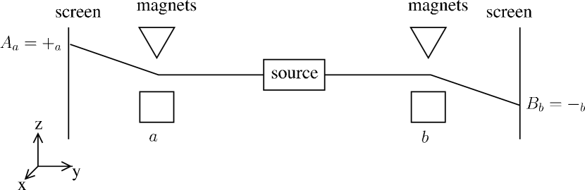
Figure 2: Setup of the EPR-Bohm experiment.

Consider the so-called EPR-Bohm (EPRB) experiment (?, ?, ?). Two spin-$\frac{1}{2}$ particles in the singlet state

$$|\Psi\rangle=\frac{1}{\sqrt{2}}\left(|\!\uparrow\downarrow\rangle-|\!\downarrow\uparrow\rangle\right)$$ (1)

are separated such that one particle moves to the measurement apparatus of Alice on the left and the other particle to the measurement apparatus of Bob on the right (see figure 2). The experimenter can arbitrarily choose the direction in which the spin is measured with a Stern-Gerlach magnet.

The event that Alice’s (Bob’s) measurement apparatus is set to measure the spin in direction $a$ ($b$) is symbolized by $a$ ($b$). $A_{a}$ ($B_{b}$) symbolizes the measurement outcome of Alice (Bob) for a measurement in direction $a$ ($b$). For each direction, there are two possible measurement outcomes: spin up ($A_{a}=+_{a}$, $B_{b}\!=\!+_{b}$) and spin down ($A_{a}=-_{a}$, $B_{b}\!=\!-_{b}$). We will always interpret these events also as elements of a Boolean algebra $\Omega$ with a classical probability measure $p$, constituting a classical probability space $(\Omega,p)$. E.g.

$$p(A_{a}B_{b}|ab)$$ (2)

denotes the probability that Alice’ measurement outcome is $A_{a}$ and Bob’s $B_{b}$, when measuring in the directions $a$ (Alice) and $b$ (Bob). We will often use the notation

$$p_{a,b}(\dots):=p(\dots|ab),$$ (3)

with which we can write (2) as

$$p_{a,b}(A_{a}B_{b}).$$ (4)

These probabilities are predicted by quantum mechanics as

$$p_{a,b}(+_{a}+_{b}) =\frac{1}{2}\sin^{2}\frac{\varphi_{a,b}}{2},$$ (5)

$$p_{a,b}(-_{a}-_{b}) =\frac{1}{2}\sin^{2}\frac{\varphi_{a,b}}{2},$$ (6)

$$p_{a,b}(+_{a}-_{b}) =\frac{1}{2}\cos^{2}\frac{\varphi_{a,b}}{2},$$ (7)

$$p_{a,b}(-_{a}+_{b}) =\frac{1}{2}\cos^{2}\frac{\varphi_{a,b}}{2},$$ (8)

where $\varphi_{a,b}$ denotes the angle between the two measurement directions $a$ and $b$. Also, the outcomes on each side are predicted separately to be completely random:

$$p_{a,b}(A_{a})=\frac{1}{2},$$ (9)

$$p_{a,b}(B_{b})=\frac{1}{2}.$$ (10)

3 Proof of a Bell-type theorem

We will first introduce our assumptions (sections 3.1 and 3.2). In the literature on Bell-type theorems, there is a huge amount of work devoted to the discussion of the assumptions. We do not intend to contribute to this discussion here. Rather, we will discuss the new elements in our set of assumptions. First, we will see that the first three assumptions imply the existence of a common cause which screens off the correlations in question. As in ? (?), the new and crucial thing here is that, in contrast to other derivations, we do not demand a single common cause for all the different correlations. Second, since we now have several different common causes, we need to adjust some assumptions (4 and 5) to this new situation. The comments on the remaining assumptions are there for the sake of clarity and not intended to contribute to the ongoing debate.

3.1 Locality and Causality

The correlation between ‘heads up’ and ‘tails down’ when tossing a coin is explained by the identity of the instances of the respective events: Every instance of ‘heads up’ is also an instance of ‘tails down’, and vice versa. Large spatial separation of coinciding instances of $A_{a}$ and $B_{b}$ suggests that such is not the case in the EPRB setup:

Assumption 1.

The coinciding instances of the events $A_{a}$ and $B_{b}$ are distinct.

Given this assumption, we can express

Assumption 2.

No $A_{a}$ or $B_{b}$ is causally relevant for the other.

This assumption is supported by the fact that the measurements can be made such that in each run of the experiment the instance of $A_{a}$ is space-like separated from the instance of $B_{b}$. If it were violated and if a cause temporally precedes its effects, the direction of causation would depend on the chosen inertial frame.

Assumption 3 (PCC).

If two events $A$ and $B$ with distinct coinciding instances are correlated and neither $A$ is causally relevant for $B$ nor vice versa, then there exists a partition $C=\{C_{i}\}_{i\in I}$ of $\Omega$, a common cause, such that

$$p(AB|C_{i})=p(A|C_{i})p(B|C_{i}),\qquad\forall i\in I.$$

We will assume the cardinality of $I$ to be countable. The common cause can alternatively be thought of as a variable (the “hidden” variable) taking on the elements of the partition as values. Thus, when we say “the value of the common cause”, we refer to an element of the partition. In the original formulation, Reichenbach used a partition with two elements, which is here generalized to a partition with countably many elements.
Now, as can be seen from equations (5)-(10), in general, the event $A_{a}$ is correlated with event $B_{b}$:

$$p_{a,b}(A_{a}B_{b})\neq p_{a,b}(A_{a})p_{a,b}(B_{b}),\mbox{ except for }\varphi_{a,b}=\frac{\pi}{2}\mod\pi.$$ (11)

With assumptions 1 and 2, PCC demands the existence of a common cause $C^{abAB}=\{C_{i}^{abAB}\}_{i\in I^{abAB}}$ which screens off the correlation:

$$p_{a,b}(A_{a}B_{b}|C_{i}^{abAB})=p_{a,b}(A_{a}|C_{i}^{abAB})p_{a,b}(B_{b}|C_{i}^{abAB}),\quad\forall i\in I^{abAB}.$$ (12)

As in ? (?) there is a common cause $C^{abAB}$ for each quadruple of measurement directions and outcomes $(a,b,A_{a},B_{b})$. That is different from other derivations, where a single common cause $\{C_{i}\}_{i\in I}$ is stipulated for all correlated events:

$$p_{a,b}(A_{a}B_{b}|C_{i})=p_{a,b}(A_{a}|C_{i})p_{a,b}(B_{b}|C_{i}),\quad\forall i\in I.$$ (13)

That such a common common cause (obeying (13)) was assumed in Bell-type theorems was pointed out and criticized by ? (?) and ? (?).

Mathematically, (13) is stronger than (12). Indeed, as already pointed out by ? (?) (p. 123), to get from (12) to (13) one needs at least one further assumption (see also ? (?), p. 15 et seq., and ? (?), p. 532 et seq.). The additional assumption states that the statistical independence in (12) does not get disrupted if one (additionally to $C_{i}^{abAB}$) conditionalizes on other events which are not causally relevant for $A_{a}$ and $B_{b}$. We do not have any strong argument for or against this assumption. To be sure, there are arguments which are brought forward in the literature in favour of it (see e.g. ? (?), ? (?), and ? (?)). But we think it is fair to say that the issue is contentious (see e.g. ? (?)). And, since we only need (12) for our derivation, we do not need to take sides on this question.

Assumption 4 (LOC).

$$p(A_{a}|abC_{i}^{abAB}) =p(A_{a}|aC_{i}^{abAB}),$$ (14)

$$p(B_{b}|abC_{i}^{abAB}) =p(B_{b}|bC_{i}^{abAB}).$$ (15)

This assumptions is meant to prevent the possibility of superluminal causation. Rather than to justify LOC, we will recall the justification of the analogue of it in the traditional derivations and show that the same justification works in our case as well. In this way, we back up our minimality claim.

In the traditional derivations, there is just one common cause. The condition then reads

$$p(A_{a}|abC_{i}) =p(A_{a}|aC_{i}),\quad\mbox{and}$$

$$p(B_{b}|abC_{i}) =p(B_{b}|bC_{i})\quad\mbox{(for all values of $a$, $b$, $A_{a}$ and $B_{b}$)}.$$ (16)

The canonical justification of (3.1) runs along the following lines. One first notes that the EPRB experiment can be set up such that the measurement outcome $A_{a}$ ($B_{b}$) and the choice of the measurement setting $b$ ($a$) are space-like separated. If Alice knew the value of the common cause (which, say, is part of her past light-cone) and (3.1) did not hold, Bob could send Alice a signal superluminally by setting up a measurement direction, since this would alter the corresponding probability of Alice’ measurement outcome. Now we do no longer have just one single common cause for all correlations but one for each. Nonetheless, the justification given above works all the same. In the sentence

“If Alice knew the value of the common cause (which, say, is part of her past light-cone) and (3.1) did not hold, Bob could send Alice a signal superluminally by setting up a measurement direction, since this would alter the corresponding probability of Alice’ measurement outcome.”,

just replace the italics with “the value of a common cause”.

3.2 Common causes for the maximal correlations

In their derivation ? (?) exploit that the screening-off condition entails that common causes of perfect correlations determine the effects. The slightest deviation from

$$p_{a=b}(+_{a}|-_{b})=p_{a=b}(+_{b}|-_{a})=1.$$ (17)

leads to a breakdown of that type of derivation. Of course, equation (17) is true according to QM and any apparent violation in actual experiments may be attributed to experimental shortcomings, for instance that, in practice, the measurement devices are never set up perfectly parallel.

Nevertheless, we would like to do without this assumption. Our motivation for this is twofold. First, there are theoretical grounds on which to expect a violation of the quantum mechanical prediction of perfect correlations. Theoretical work in the different approaches to quantum gravity suggests that tiny violations of Lorentz group invariance are to be expected. Seen as an implication of rotation invariance, (17) would not be warranted any more. The second motivation has to do with the prominent claim that Bell-type theorems rule out the existence of empirically adequate local hidden-variable models on empirical grounds alone. However, if besides the assumptions that define the model as a local hidden-variable model, the only constraint were empirical adequacy, PCORR should not be assumed, because small violations of it are consistent with empirical data.

These considerations motivate a weakening of (17) such that we just take the maximal correlations available, without assuming that they are perfect. We do this as follows. For each pair of measurement directions $(a,b)$, we parametrize the conditional probabilities $p_{a,b}(+_{a}|-_{b})$ and $p_{a,b}(+_{b}|-_{a})$ as

$$p_{a,b}(+_{a}|-_{b}) =1-\epsilon_{a,b},$$

$$p_{a,b}(+_{b}|-_{a}) =1-\epsilon_{b,a},\mbox{ with }\epsilon_{a,b},\epsilon_{b,a}\in[0,1].$$ (18)

We will call the set of all measurement directions of Alice (of Bob) $D_{A}$ ($D_{B}$). For each measurement direction $a\in D_{A}$ ($b\in D_{B}$), we pick out the measurement direction $\dot{a}\in D_{B}$ ($\dot{b}\in D_{A}$) for which $p_{a,b}(+_{a}|-_{b})$ ($p_{a,b}(+_{b}|-_{a})$) takes on its maximal value, or, equivalently, $\epsilon_{a,b}$ ($\epsilon_{b,a}$) takes on its minimal value. If the same minimal value is taken on for more than one direction, we make an arbitrary choice. We denote this minimal value with $\epsilon_{a}$ ($\epsilon_{b}$):

$$\epsilon_{a}: =\min_{b}\{\epsilon_{a,b}\},$$

$$\epsilon_{b}: =\min_{a}\{\epsilon_{b,a}\}.$$ (19)

Thus, we have

$$p_{a,\dot{a}}(+_{a}|-_{a}) =1-\epsilon_{a},$$

$$p_{\dot{b},b}(+_{b}|-_{b}) =1-\epsilon_{b}.$$ (20)

Because of assumptions 1 to 3, we have (in the notation of formula (12)) a common cause $\{C_{i}^{a\dot{a}+-}\}_{i\in I^{a\dot{a}+-}}$ ($\{C_{i}^{\dot{b}b-+}\}_{i\in I^{\dot{b}b-+}}$) for the events $+_{a}$ and $-_{\dot{a}}$ ($+_{b}$ and $-_{\dot{b}}$). Henceforth, we will use the short hand $\{C_{i}^{a}\}_{i\in I^{a}}$ ($\{C_{i}^{b}\}_{i\in I^{b}}$) for $\{C_{i}^{a\dot{a}+-}\}_{i\in I^{a\dot{a}+-}}$ ($\{C_{i}^{\dot{b}b-+}\}_{i\in I^{\dot{b}b-+}}$). With this notation, we get:

$$p_{a,\dot{a}}(+_{a},-_{a}|C^{a}_{i}) =p_{a,\dot{a}}(+_{a}|C^{a}_{i})p_{a,\dot{a}}(-_{a}|C^{a}_{i}),\forall i\in I^{a},$$

$$p_{\dot{b},b}(-_{b},+_{b}|C^{b}_{i}) =p_{\dot{b},b}(-_{b}|C^{b}_{i})p_{\dot{b},b}(+_{b}|C^{b}_{i}),\forall i\in I^{b}.$$ (21)

Assumption 5.

$$p(aC_{i}^{a}) =p(a)p(C_{i}^{a})$$ (22)

$$p(bC_{i}^{b}) =p(b)p(C_{i}^{b})$$ (23)

$$p(abC_{i}^{a}) =p(ab)p(C_{i}^{a}),$$ (24)

$$p(abC_{i}^{b}) =p(ab)p(C_{i}^{b}),$$ (25)

$$p(abC_{i}^{a}C_{j}^{b}) =p(ab)p(C_{i}^{a}C_{j}^{b}).$$ (26)

With this assumption one would like to exclude that the common causes are causally relevant for the setting of the measurement apparatuses or vice versa. Furthermore, one would like to exclude a common cause for these factors.

3.3 Constraints for $p_{a,b}(+_{a}+_{b})$, $p(+_{a}|a)$, and $p(+_{b}|b)$

To obtain a Bell-type inequality we need an upper and a lower bound for

$$p_{a,b}(+_{a}+_{b}),p(+_{a}|a),\mbox{ and }p(+_{b}|b).$$ (27)

We will need the following proposition.

Proposition 1.

Let two events $A$ and $B$ with $p(A)=p(B)=0.5$ be almost perfectly correlated ($p(A|B)=1-\epsilon$) and assume a common cause $C=\{C_{i}\}_{i\in I}$, such that

$$p(AB|C_{i})=p(A|C_{i})p(B|C_{i}),\forall i\in I.$$ (28)

Then

$$\sum_{i\in I_{1}}p(C_{i})-\sqrt{\epsilon}\leq p(A)<\sum_{i\in I_{1}}p(C_{i})+4\sqrt{\epsilon}-2\epsilon,$$ (29)

where

$$I_{1} :=\{i\in I:p(A|C_{i})\geq 1-\sqrt{\epsilon}\}.$$ (30)

We prove proposition 1 in appendix A.

With the definition

$$C:=\vee_{i\in I_{1}}C_{i},$$ (31)

equation (29) reads

$$p(C)-\sqrt{\epsilon}\leq p(A)<p(C)+4\sqrt{\epsilon}-2\epsilon,$$ (32)

or, equivalently,

$$p(A)-4\sqrt{\epsilon}+2\epsilon<p(C)\leq p(A)+\sqrt{\epsilon}.$$ (33)

We define

$$I_{1}^{a} :=\{i\in I^{a}:p_{a,\dot{a}}(+_{a}|C_{i}^{a})\stackrel{{\scriptstyle(*)}}{{=}}p(+_{a}|aC_{i}^{a})\geq 1-\sqrt{\epsilon_{a}}\},$$

$$C^{a} :=\vee_{i\in I_{1}^{a}}C_{i}^{a},$$

$$I_{1}^{b} :=\{i\in I^{b}:p_{\dot{b},b}(+_{b}|bC_{i}^{b})\stackrel{{\scriptstyle(*)}}{{=}}p(+_{b}|bC_{i}^{b})\geq 1-\sqrt{\epsilon_{b}}\},$$

$$C^{b} :=\vee_{i\in I_{1}^{b}}C_{i}^{b}.$$ (34)

In $(*)$, we use LOC.

With the substitutions

$$p(\dots) \rightarrow p_{a,\dot{a}}(\dots), \qquad p(\dots) \rightarrow p_{\dot{b},b}(\dots),$$

$$A \rightarrow+_{a}, \quad A \rightarrow+_{b},$$

$$B \rightarrow-_{\dot{a}}, \quad B \rightarrow-_{\dot{b}},$$

$$C \rightarrow C^{a}, \quad C \rightarrow C^{b},$$

$$\epsilon \rightarrow\epsilon_{a}, \quad\epsilon \rightarrow\epsilon_{b},$$ (35)

we get

$$p_{a,\dot{a}}(+_{a})-4\sqrt{\epsilon_{a}}+2\epsilon_{a} <p_{a,\dot{a}}(C^{a}) \leq p_{a,\dot{a}}(+_{a})+\sqrt{\epsilon_{a}},$$

$$p_{\dot{b},b}(+_{b})-4\sqrt{\epsilon_{b}}+2\epsilon_{b} <p_{\dot{b},b}(C^{b}) \leq p_{\dot{b},b}(+_{b})+\sqrt{\epsilon_{b}}.$$ (36)

Using assumption 4, 5, and the definition

$$\epsilon:=\max_{a,b}\{\epsilon_{a},\epsilon_{b}\},$$ (37)

we get

$$p(+_{a}|a)-\Delta^{+} <p(C^{a}) \leq p(+_{a}|a)+\Delta^{-},$$

$$p(+_{b}|b)-\Delta^{+} <p(C^{b}) \leq p(+_{b}|b)+\Delta^{-},$$ (38)

with

$$\Delta^{+} =4\sqrt{\epsilon}-2\epsilon,$$

$$\Delta^{-} =\sqrt{\epsilon}.$$ (39)

Using again assumptions 4 and 5, the following bounds for $p(+_{a}+_{b}|ab)$ can be derived (this is shown in appendix B):

$$p_{a,b}(+_{a}+_{b})-\Delta_{a,b}^{+}<p(C^{a}C^{b})\leq p_{a,b}(+_{a}+_{b})+\Delta_{a,b}^{-},$$ (40)

with

$$\Delta_{a,b}^{+} =\frac{(p(a)+p(b))(5\sqrt{\epsilon}-2\epsilon)}{p(ab)},$$

$$\Delta_{a,b}^{-} =\frac{(p(a)+p(b))\sqrt{\epsilon}}{p(ab)}.$$ (41)

3.4 A weak Clauser-Horne inequality

In the next step, we make use of a constraint, which holds for the probabilities of arbitrary events. For events $A$ and $B$ to be elements of a classical probability space, it is not enough that

$$0\leq p(A)\leq 1,$$

$$0\leq p(B)\leq 1,$$

$$0\leq p(AB)\leq 1,$$ (42)

and

$$p(AB) \leq p(A),$$

$$p(AB) \leq p(B).$$ (43)

We note first, that (“$\bar{A}$” means “not $A$”)

$$p(AB)+p(A\bar{B})+p(\bar{A}B)+p(\bar{A}\bar{B})=1.$$ (44)

It is also

$$p(A) =p(AB)+p(A\bar{B}),\quad\mbox{and}$$

$$p(B) =p(AB)+p(\bar{A}B),$$ (45)

and hence

$$p(A)+p(B)-p(AB)=p(AB)+p(A\bar{B})+p(\bar{A}B),$$ (46)

which implies with equation (44)

$$0\leq p(A)+p(B)-p(AB)\leq 1.$$ (47)

For more than two events there are more constraints in the form of such inequalities. For four events $A$, $A^{\prime}$, $B$ and $B^{\prime}$, one constraint reads

$$-1\leq p(AB)+p(AB^{\prime})+p(A^{\prime}B^{\prime})-p(A^{\prime}B)-p(A)-p(B^{\prime})\leq 0.$$ (48)

This is the Clauser-Horne inequality (?, ?), which we prove in appendix C. This inequality is an a priori constraint for arbitrary events. Hence, for the measurement directions $1,2\in D_{A}$ and $3,4\in D_{B}$, it is also

$$-1\leq p(C^{1}C^{3})+p(C^{1}C^{4})+p(C^{2}C^{4})$$

$$-p(C^{2}C^{3})-p(C^{1})-p(C^{4})$$

$$\leq 0.$$ (49)

Together with inequality (40)

$$p_{a,b}(+_{a}+_{b})-\Delta_{a,b}^{+}<p(C^{a}C^{b})\leq p_{a,b}(+_{a}+_{b})+\Delta_{a,b}^{-}$$

and inequality (3.3)

$$p(+_{a}|a)-\Delta^{+} <p(C^{a}) \leq p(+_{a}|a)+\Delta^{-},$$

$$p(+_{b}|b)-\Delta^{+} <p(C^{b}) \leq p(+_{b}|b)+\Delta^{-}$$

one gets

$$-1-\Delta_{1,3}^{-} -\Delta_{1,4}^{-}-\Delta_{2,4}^{-}-\Delta_{2,3}^{+}-2\Delta^{+}$$

$$< p_{1,3}(+_{1}+_{3})+p_{1,4}(+_{1}+_{4})+p_{2,4}(+_{2}+_{4})$$

$$-p_{2,3}(+_{2}+_{3})-p(+_{1}|1)-p(+_{4}|4)$$

$$< \Delta_{1,3}^{+}+\Delta_{1,4}^{+}+\Delta_{2,4}^{+}+\Delta_{2,3}^{-}+2\Delta^{-},$$ (50)

with

$$\Delta_{a,b}^{-} =\frac{(p(a)+p(b))\sqrt{\epsilon}}{p(ab)},$$

$$\Delta_{a,b}^{+} =\frac{(p(a)+p(b))(5\sqrt{\epsilon}-2\epsilon)}{p(ab)},$$

$$\Delta^{-} =\sqrt{\epsilon},$$

$$\Delta^{+} =4\sqrt{\epsilon}-2\epsilon.$$ (51)

Note that this inequality reduces to the Clauser-Horne inequality for $\epsilon=0$.

3.5 Contradiction

The predicted values of $p_{1,3}(+_{1},+_{3})$, $p_{1,4}(+_{1},+_{4})$, $p_{2,4}(+_{2},+_{4})$ and $p_{2,3}(+_{2},+_{3})$ by QM are such that the maximal violation for the lower bound of (3.4) occurs (among others) for the angles $\varphi_{1,3}=\varphi_{1,4}=\varphi_{2,4}=\frac{\pi}{4}$ and $\varphi_{2,3}=\frac{3\pi}{4}$:

$$-1-\Delta_{1,3}^{-} -\Delta_{1,4}^{-}-\Delta_{2,4}^{-}-\Delta_{2,3}^{+}-\Delta^{+}-\Delta^{+}$$

$$< p_{1,3}(+_{1}+_{3})+p_{1,4}(+_{1}+_{4})+p_{2,4}(+_{2},+_{4})$$

$$-p_{2,3}(+_{2}+_{3})-p(+_{1}|1)-p(+_{4}|4)=-\frac{\sqrt{2}+1}{2}.$$ (52)

The maximal violation for the upper bound occurs (among others) for the angles $\varphi_{1,3}=\varphi_{2,4}=\frac{3\pi}{4}$, $\varphi_{1,4}=\frac{5\pi}{4}$ and $\varphi_{2,3}=\frac{\pi}{4}$:

$$\frac{\sqrt{2}-1}{2}= p_{1,3}(+_{1}+_{3})+p_{1,4}(+_{1}+_{4})+p_{2,4}(+_{2}+_{4})$$

$$-p_{2,3}(+_{2}+_{3})-p(+_{1}|1)-p(+_{4}|4)$$

$$< \Delta_{1,3}^{+}+\Delta_{1,4}^{+}+\Delta_{2,4}^{+}+\Delta_{2,3}^{-}+\Delta^{-}+\Delta^{-},$$ (53)

With $p(ab)=\frac{1}{4}$ and $p(a)=p(b)=\frac{1}{2}$, one has

$$\Delta_{a,b}^{-}=4\sqrt{\epsilon}\quad\mbox{and}\quad\Delta_{a,b}^{+}=20\sqrt{\epsilon}-8\epsilon.$$ (54)

With the chosen angles and measurement probabilities one gets

$$\frac{\sqrt{2}-1}{2}<40\sqrt{\epsilon}-12\epsilon.$$ (55)

for the lower bound. This inequality is violated for

$$\epsilon\leq\epsilon^{l}_{\max},\quad\epsilon^{l}_{\max}=2.689\cdot 10^{-5}.$$ (56)

The inequality for the upper bound reads

$$\frac{\sqrt{2}-1}{2}<66\sqrt{\epsilon}-24\epsilon,$$ (57)

which is violated for

$$\epsilon\leq\epsilon^{u}_{\max},\quad\epsilon^{u}_{\max}=9.869\cdot 10^{-6}.$$ (58)

Thus the quantum mechanical predictions contradict the predictions of a hidden variable model obeying our assumptions for

$$\epsilon\leq\epsilon^{l}_{\max}=2.698\cdot 10^{-5}.$$ (59)

4 Discussion

Figure 3: Comparison with other constraints.

Even though the four sets of assumptions in ? (?), ? (?), ? (?) and ? (?) (see figure 1) differ, they all imply the same constraints on the correlations as expressed in the Clauser-Horne inequality.

One of the questions left open by ? (?) is what constraints are implied without assuming the existence of perfectly correlated events. Since with a slightest deviation from perfect correlations the proof by ? (?) breaks down, it gives no hint as to whether the same Bell-type constraints follow nor whether a contradiction to QM is entailed at all. In the present paper we have given a partial answer to that question.

The inequality we get at the end of our derivation is stronger than the quantum mechanical predictions (for $\epsilon\leq\epsilon^{l}_{\max}$), but weaker than the Clauser-Horne inequality (for $\epsilon>0$). Thus, the weakening of the assumptions is also reflected in a resulting weakening of the constraints. Note however that we did not prove that this weakening is really an implication of our assumptions. What we have shown is only that the conditional probabilities at least have to obey the constraint (3.4). To prove the stronger proposition, one could try to construct a separate common cause model obeying all our assumptions that violates the Clauser-Horne inequality without correction terms, but does not violate the weak Clauser-Horne inequality.

Now, we would like to compare our inequality to other prominent constraints (see figure 3). Even though Bell’s theorem excludes models which obey local causality, the predictions of QM for $p(A_{a}B_{b}|ab)$ still obey the no-signalling constraint

$$\sum_{B_{b}}p(A_{a}B_{b}|ab) =\sum_{B_{b}}p(A_{a}B_{b}|ab^{\prime}),$$

$$\sum_{A_{a}}p(A_{a}B_{b}|ab) =\sum_{A_{a^{\prime}}}p(A_{a^{\prime}}B_{b}|a^{\prime}b),$$ (60)

which states that the probability of the measurement outcome on one side does not depend on the measurement direction on the other side (given the quantum mechanical state of the system). Moreover, there are some correlations obeying no-signalling which are not permitted by quantum mechanics. The bounds, which are allowed by quantum mechanics, were first derived by ? (?). Notoriously, still more constraining are the Bell inequalities. The situation is drawn schematically in figure 3. The boarder at the margin is the least constraining coming from the no-signalling condition (4). Next is the Tsirelson-bound, which is again weaker than the bound coming from the Clauser-Horne inequality (local causality). The bound coming from inequality (3.4) lies between the Tsirelson bound and the bound coming from the Clauser-Horne inequality, depending on the value of $\epsilon$. For $\epsilon\neq 0$ there are quantum mechanical states which do violate the Clauser-Horne inequality but not (3.4). This reveals the following a priori possibility. As ? (?) showed, the correlations coming from pure entangled states always violate the Clauser-Horne inequality. For $\epsilon\neq 0$, Gisin’s argument is not sufficient to conclude that all entangled states violate inequality (3.4). Hence, it is an open question, whether or not there exist models obeying all our assumptions, for the correlations of some entangled pure states.

Even though $\epsilon^{l}_{\max}$ is not zero, it is still very small. Particularly, violations of correlations deviating only through $\epsilon^{l}_{\max}$ from being perfect, can experimentally not be ruled out. This means that we cannot rule out the existence of an empirically adequate hidden variable model obeying all our assumptions. On the other hand, from a theoretical point of view, a deviation from perfect correlation of order $\epsilon^{l}_{\max}$ is rather big. Modulo some theoretical assumptions, any non-vanishing $\epsilon$ can be interpreted as a violation of rotation invariance (see section 3.3), which moreover induces a violation of Lorentz invariance. Triggered by theoretical works in various approaches to quantum gravity, which either imply violations of Lorentz invariance or render such a violation natural, there has been a tremendous experimental effort for finding signatures of such violations during the last ten years or so (for a recent review, see e.g. ? (?)). The constraints coming from negative results of such experiments are rather strong. In view of these findings, one would expect $\epsilon$ to be smaller than $\epsilon^{l}_{\max}$ and the inequality (3.4) to be violated.

Appendix A Proof of proposition 1

Proposition 1.

Let two events $A$ and $B$ with $p(A)=p(B)=0.5$ be almost perfectly correlated ($p(A|B)=1-\epsilon$) and assume a common cause $C=\{C_{i}\}_{i\in I}$, such that

$$p(AB|C_{i})=p(A|C_{i})p(B|C_{i}),\quad\forall i\in I.$$ (61)

Then

$$\sum_{i\in I_{1}}p(C_{i})-\sqrt{\epsilon}\leq p(A)<\sum_{i\in I_{1}}p(C_{i})+4\sqrt{\epsilon}-2\epsilon,$$ (62)

where

$$I_{1} :=\{i\in I:p(A|C_{i})\geq 1-\sqrt{\epsilon}\}.$$ (63)

Proof.

We will partition $I$ into the following three subsets:

$$I_{1} :=\{i\in I:p(A|C_{i})\geq 1-\sqrt{\epsilon}\},$$

$$I_{2} :=\{i\in I:\sqrt{\epsilon}<p(A|C_{i})<1-\sqrt{\epsilon}\},$$

$$I_{3} :=\{i\in I:p(A|C_{i})\leq\sqrt{\epsilon}\}.$$ (64)

It is

$$p(A)=\sum_{i\in I_{1}}p(A|C_{i})p(C_{i})+\sum_{i\in I_{2}}p(A|C_{i})p(C_{i})+\sum_{i\in I_{3}}p(A|C_{i})p(C_{i}).$$ (65)

With the definitions (A) the following inequalities hold:

$$p(A) \geq\sum_{i\in I_{1}}p(A|C_{i})p(C_{i})\geq(1-\sqrt{\epsilon})\sum_{i\in I_{1}}p(C_{i})\geq\sum_{i\in I_{1}}p(C_{i})-\sqrt{\epsilon},$$

$$p(A) \leq\sum_{i\in I_{1}}p(C_{i})+\sum_{i\in I_{2}}p(A|C_{i})p(C_{i})+\sqrt{\epsilon}.$$ (66)

Hence, to complete the proof we have to show that

$$\sum_{i\in I_{2}}p(A|C_{i})p(C_{i})<3\sqrt{\epsilon}-2\epsilon.$$ (67)

It is

$$\frac{\epsilon}{2}=\underbrace{p(A)}_{\frac{1}{2}}-\underbrace{p(AB)}_{\frac{1-\epsilon}{2}} =\sum_{i\in I}\left[p(A|C_{i})-p(AB|C_{i})\right]p(C_{i})$$

$$\stackrel{{\scriptstyle(*)}}{{=}}\sum_{i\in I}\left[p(A|C_{i})-p(A|C_{i})p(B|C_{i})\right]p(C_{i})$$

$$=\sum_{i\in I}p(A|C_{i})\left[1-p(B|C_{i})\right]p(C_{i}),$$ (68)

where we used (61) to get equality $(*)$. Since everything is symmetric in $A$ and $B$, the same holds if one exchanges $A$ and $B$ for each other. We thus have

$$\sum_{i\in I}p(A|C_{i})\left[1-p(B|C_{i})\right]p(C_{i}) =\frac{\epsilon}{2},$$ (69)

$$\sum_{i\in I}p(B|C_{i})\left[1-p(A|C_{i})\right]p(C_{i}) =\frac{\epsilon}{2}.$$ (70)

Since all terms in the sums on the L.H.S. of eq. (69, 70) are positive, the following inequalities hold for all subsets $I^{\subset}$ of the value space $I$:

$$0\leq\sum_{i\in I^{\subset}}p(A|C_{i})\left[1-p(B|C_{i})\right]p(C_{i}) \leq\frac{\epsilon}{2},\quad\forall I^{\subset}\subset I,$$ (71)

$$0\leq\sum_{i\in I^{\subset}}p(B|C_{i})\left[1-p(A|C_{i})\right]p(C_{i}) \leq\frac{\epsilon}{2},\quad\forall I^{\subset}\subset I.$$ (72)

Subtracting (71) from (72), one gets

$$\left|\sum_{i\in I^{\subset}}\left[p(A|C_{i})-p(B|C_{i})\right]p(C_{i})\right|\leq\frac{\epsilon}{2},\quad\forall I^{\subset}\subset I.$$ (73)

With the definitions

$$I_{2}^{A\geq B} :=\left\{i\in I_{2}:p(A|C_{i})\geq p(B|C_{i})\right\},$$ (74)

$$I_{2}^{A<B} :=\left\{i\in I_{2}:p(A|C_{i})<p(B|C_{i})\right\}$$ (75)

and applying (73) for these sets, one gets

$$\left|\sum_{i\in I_{2}^{A\geq B}}\left[p(A|C_{i})-p(B|C_{i})\right]p(C_{i})\right| =\sum_{i\in I_{2}^{A\geq B}}\left|p(A|C_{i})-p(B|C_{i})\right|p(C_{i})\leq\frac{\epsilon}{2},$$ (76)

$$\left|\sum_{i\in I_{2}^{A<B}}\left[p(A|C_{i})-p(B|C_{i})\right]p(C_{i})\right| =\sum_{i\in I_{2}^{A<B}}\left|p(A|C_{i})-p(B|C_{i})\right|p(C_{i})\leq\frac{\epsilon}{2}.$$ (77)

Adding these two inequalities, one gets:

$$\sum_{i\in I_{2}}\left|p(A|C_{i})-p(B|C_{i})\right|p(C_{i})\leq\epsilon.$$ (78)

We partition $I_{2}$ in the following two subsets:

$$I_{2}^{\geq\sqrt{\epsilon}} :=\left\{i\in I_{2}:\left|p(A|C_{i})-p(B|C_{i})\right|\geq\frac{\sqrt{\epsilon}}{2}\right\},$$

$$I_{2}^{<\sqrt{\epsilon}} :=\left\{i\in I_{2}:\left|p(A|C_{i})-p(B|C_{i})\right|<\frac{\sqrt{\epsilon}}{2}\right\}.$$ (79)

From

$$\sum_{i\in I_{2}^{\geq\sqrt{\epsilon}}}\left|p(A|C_{i})-p(B|C_{i})\right|p(C_{i})\geq\frac{\sqrt{\epsilon}}{2}\sum_{i\in I_{2}^{\geq\sqrt{\epsilon}}}p(C_{i})$$ (80)

together with (78), we get

$$\sum_{i\in I_{2}^{\geq\sqrt{\epsilon}}}p(C_{i})\leq 2\sqrt{\epsilon}.$$ (81)

Remember, that we want to derive an upper bound for

$$\sum_{i\in I_{2}}p(A|C_{i})p(C_{i}).$$ (82)

With (81), we already have

$$\sum_{i\in I_{2}}p(A|C_{i})p(C_{i}) =\sum_{i\in I_{2}^{\geq\sqrt{\epsilon}}}p(A|C_{i})p(C_{i})+\sum_{i\in I_{2}^{<\sqrt{\epsilon}}}p(A|C_{i})p(C_{i})$$

$$<(1-\sqrt{\epsilon})2\sqrt{\epsilon}+\sum_{i\in I_{2}^{<\sqrt{\epsilon}}}p(A|C_{i})p(C_{i}).$$ (83)

We will use again inequality (71), this time for the set $I_{2}^{<\sqrt{\epsilon}}$:

$$\sum_{i\in I_{2}^{<\sqrt{\epsilon}}}p(A|C_{i})\left[1-p(B|C_{i})\right]p(C_{i}) \leq\frac{\epsilon}{2}.$$ (84)

Because we are looking at the subset $I_{2}^{<\sqrt{\epsilon}}$, it is

$$\sum_{i\in I_{2}^{<\sqrt{\epsilon}}}p(A|C_{i})\left[1-p(B|C_{i})\right]p(C_{i})>\sum_{i\in I_{2}^{<\sqrt{\epsilon}}}p(A|C_{i})\left[1-p(A|C_{i})-\frac{\sqrt{\epsilon}}{2}\right]p(C_{i}).$$ (85)

With (84), one gets

$$\sum_{i\in I_{2}^{<\sqrt{\epsilon}}}p(A|C_{i})\left[1-p(A|C_{i})-\frac{\sqrt{\epsilon}}{2}\right]p(C_{i}) <\frac{\epsilon}{2}.$$ (86)

Now, since $I_{2}^{<\sqrt{\epsilon}}$ is a subset of $I_{2}$, $p(A|C_{i})$ takes on values in the interval $[\sqrt{\epsilon},1-\sqrt{\epsilon}]$. One can check that each summand is certainly greater than for $p(A|C_{i})=1-\sqrt{\epsilon}$. We have

$$\sum_{i\in I_{2}^{<\sqrt{\epsilon}}}p(A|C_{i})\left[1-p(A|C_{i})-\frac{\sqrt{\epsilon}}{2}\right]p(C_{i})>(1-\sqrt{\epsilon})\frac{\sqrt{\epsilon}}{2}\sum_{i\in I_{2}^{<\sqrt{\epsilon}}}p(C_{i}).$$ (87)

We get the constraint

$$\sum_{i\in I_{2}^{<\sqrt{\epsilon}}}p(C_{i})<\frac{\sqrt{\epsilon}}{(1-\sqrt{\epsilon})}.$$ (88)

With (A) one gets

$$\sum_{i\in I_{2}}p(A|C_{i})p(C_{i})<(1-\sqrt{\epsilon})2\sqrt{\epsilon}+\sqrt{\epsilon}=3\sqrt{\epsilon}-2\epsilon,$$ (89)

which is what we wanted to show. We have

$$\sum_{i\in I_{1}}p(C_{i})-\sqrt{\epsilon}\leq p(A)<\sum_{i\in I_{1}}p(C_{i})+4\sqrt{\epsilon}-2\epsilon.$$ (90)

∎

Appendix B Bounds for $p(+_{a}+_{b}|ab)$

With (3.3) and assumption 5, we get

$$p(+_{a}|a) =p(+_{a}C^{a}|a)+p(+_{a}\overline{C^{a}}|a)<p(C^{a}|a)+4\sqrt{\epsilon}-2\epsilon$$

$$=p(+_{a}C^{a}|a)+p(\overline{+_{a}}C^{a}|a)+4\sqrt{\epsilon}-2\epsilon,$$ (91)

and hence

$$p(+_{a}a\overline{C^{a}})<p(\overline{+_{a}}aC^{a})+p(a)\left(4\sqrt{\epsilon}-2\epsilon\right).$$ (92)

Furthermore, we have

$$p(\overline{+_{a}}C^{a}|a) \stackrel{{\scriptstyle(*)}}{{=}}\sum_{i\in I_{1}^{a}}p(\overline{+_{a}}|aC^{a}_{i})p(C^{a}_{i})$$

$$=\sum_{i\in I_{1}^{a}}\left(1-p(+_{a}|aC^{a}_{i})\right)p(C^{a}_{i})$$

$$\leq\sqrt{\epsilon}\sum_{i\in I_{1}^{a}}p(C^{a}_{i})\leq\sqrt{\epsilon},$$ (93)

where we used assumption 5 to get equality $(*)$. We can write (B) as

$$p(\overline{+_{a}}aC^{a})\leq p(a)\sqrt{\epsilon},$$ (94)

such that we get from (92)

$$p(+_{a}a\overline{C^{a}}X)<p(a)\left(5\sqrt{\epsilon}-2\epsilon\right),$$ (95)

because for any $X$ and any $Y$, $p(XY)\leq p(Y)$. Next, from

$$p(+_{a}aC^{a}X)=p(aC^{a}X)-p(\overline{+_{a}}aC^{a}X)$$ (96)

together with (94) and because $p(\overline{+_{a}}aC^{a}X)\leq p(\overline{+_{a}}aC^{a})$ we get

$$p(+_{a}aC^{a}X)\geq p(aC^{a}X)-p(a)\sqrt{\epsilon}.$$ (97)

Starting from the other inequalities in (3.3), we get inequalities analogue to (95) and (97). We have

$$p(+_{a}a\overline{C^{a}}X) <p(a)\left(5\sqrt{\epsilon}-2\epsilon\right),$$ (98)

$$p(+_{b}b\overline{C^{b}}X) <p(b)\left(5\sqrt{\epsilon}-2\epsilon\right),$$ (99)

$$p(+_{a}aC^{a}X) \geq p(aC^{a}X)-p(a)\sqrt{\epsilon},$$ (100)

$$p(+_{b}bC^{b}X) \geq p(bC^{b}X)-p(b)\sqrt{\epsilon}.$$ (101)

Now, we can derive an upper bound for $p\left(+_{a}+_{b}ab\right)$, using (98) and (99):

$$\begin{split}p(+_{a}+_{b}ab)&=p(+_{a}+_{b}abC^{a})+p(+_{a}+_{b}ab\overline{C^{a}})\\ &<p(+_{a}+_{b}abC^{a})+p(a)\left(5\sqrt{\epsilon}-2\epsilon\right)\\ &<p(+_{a}+_{b}abC^{a}C^{b})+\left(p(a)+p(b)\right)\left(5\sqrt{\epsilon}-2\epsilon\right)\\ &\leq p(abC^{a}C^{b})+\left(p(a)+p(b)\right)\left(5\sqrt{\epsilon}-2\epsilon\right).\end{split}$$ (102)

Using also assumption 5, we finally obtain

$$p(+_{a}+_{b}|ab) \equiv \frac{p(+_{a}+_{b}ab)}{p(ab)}$$ (103)

$$< \frac{p(abC^{a}C^{b})+\left(p(a)+p(b)\right)(5\sqrt{\epsilon}-2\epsilon)}{p(ab)}$$

$$= p(C^{a}C^{b}|ab)+\left(p(a)+p(b)\right)\frac{5\sqrt{\epsilon}-2\epsilon}{p(ab)}$$

$$= p(C^{a}C^{b})+\left(p(a)+p(b)\right)\frac{5\sqrt{\epsilon}-2\epsilon}{p(ab)}.$$

Next, we derive a lower bound.

$$\begin{split}p(+_{a}+_{b}ab)&\geq p(+_{a}+_{b}abC^{a}C^{b})\\ &\geq p(+_{b}abC^{a}C^{b})-p(a)\sqrt{\epsilon}\\ &\geq p(abC^{a}C^{b})-\left(p(a)+p(b)\right)\sqrt{\epsilon},\end{split}$$ (104)

$$p(+_{a}+_{b}|ab) \equiv \frac{p(+_{a}+_{b}ab)}{p(ab)}$$ (105)

$$\geq p(C^{a}C^{b})-\frac{\left(p(a)+p(b)\right)\sqrt{\epsilon}}{p(ab)}.$$

(103) and (105) imply

$$p(+_{a}+_{b}|ab)-\Delta_{a,b}^{+}<p(C^{a}C^{b})\leq p(+_{a}+_{b}|ab)+\Delta_{a,b}^{-},$$ (106)

with

$$\Delta_{a,b}^{-} =\frac{\left(p(a)+p(b)\right)\sqrt{\epsilon}}{p(ab)},$$

$$\Delta_{a,b}^{+} =\frac{\left(p(a)+p(b)\right)(5\sqrt{\epsilon}-2\epsilon)}{p(ab)}.$$ (107)

Appendix C Proof of the Clauser-Horne Inequality

In this appendix we will prove inequality (48). We consider arbitrary four events $A$, $A^{\prime}$, $B$, and $B^{\prime}$ together with their complements. The sum over all $16$ possibilities equals one:

$$\sum_{a,a^{\prime},b,b^{\prime}}p(a,a^{\prime},b,b^{\prime})=1,\qquad\mbox{where}\quad a\in\{A,\bar{A}\}\quad\mbox{etc.}$$ (108)

We also have

$$p(AB)= p(AA^{\prime}BB^{\prime})+p(AA^{\prime}B\bar{B^{\prime}})+p(A\bar{A^{\prime}}BB^{\prime})+p(A\bar{A^{\prime}}B\bar{B^{\prime}}),$$

$$p(AB^{\prime})= p(AA^{\prime}BB^{\prime})+p(A\bar{A^{\prime}}BB^{\prime})+p(AA^{\prime}\bar{B}B^{\prime})+p(A\bar{A^{\prime}}\bar{B}B^{\prime}),$$

$$p(A^{\prime}B^{\prime})= p(AA^{\prime}BB^{\prime})+p(AA^{\prime}\bar{B}B^{\prime})+p(\bar{A}A^{\prime}BB^{\prime})+p(\bar{A}A^{\prime}\bar{B}B^{\prime}),$$

$$p(A^{\prime}B)= p(AA^{\prime}BB^{\prime})+p(AA^{\prime}B\bar{B^{\prime}})+p(\bar{A}A^{\prime}BB^{\prime})+p(\bar{A}A^{\prime}B\bar{B^{\prime}}),$$

$$p(A)= p(AA^{\prime}BB^{\prime})+p(AA^{\prime}B\bar{B^{\prime}})+p(A\bar{A^{\prime}}BB^{\prime})+p(A\bar{A^{\prime}}B\bar{B^{\prime}})$$

$$+p(AA^{\prime}\bar{B}B^{\prime})+p(AA^{\prime}\bar{B}\bar{B^{\prime}})+p(A\bar{A^{\prime}}\bar{B}B^{\prime})+p(A\bar{A^{\prime}}\bar{B}\bar{B^{\prime}}),$$

$$p(B^{\prime})= p(AA^{\prime}BB^{\prime})+p(A\bar{A^{\prime}}BB^{\prime})+p(AA^{\prime}\bar{B}B^{\prime})+p(A\bar{A^{\prime}}\bar{B}B^{\prime})$$

$$+p(\bar{A}A^{\prime}BB^{\prime})+p(\bar{A}\bar{A^{\prime}}BB^{\prime})+p(\bar{A}A^{\prime}\bar{B}B^{\prime})+p(\bar{A}\bar{A^{\prime}}\bar{B}B^{\prime}).$$ (109)

Thus

$$p(AB)+ p(AB^{\prime})+p(A^{\prime}B^{\prime})-p(A^{\prime}B)-p(A)-p(B^{\prime})$$

$$= -\big{[}p(AA^{\prime}B\bar{B^{\prime}})+p(AA^{\prime}\bar{B}\bar{B^{\prime}})+p(A\bar{A^{\prime}}\bar{B}B^{\prime})+p(A\bar{A^{\prime}}\bar{B}\bar{B^{\prime}})$$

$$+p(\bar{A}A^{\prime}BB^{\prime})+p(\bar{A}A^{\prime}B\bar{B^{\prime}})+p(\bar{A}\bar{A^{\prime}}BB^{\prime})+p(\bar{A}\bar{A^{\prime}}\bar{B}B^{\prime})\big{]}.$$ (110)

Because each term appears only once on the R.H.S. of equation (C), equation (108) implies the Clauser-Horne inequality:

$$-1\leq p(AB)+p(AB^{\prime})+p(A^{\prime}B^{\prime})-p(A^{\prime}B)-p(A)-p(B^{\prime})\leq 0.$$ (111)

References

- BellBell Bell, J. S. (1964). On the Einstein-Podolsky-Rosen Paradox. Physics, 1, 195. (Reprinted in (?, ?, pp. 14-21))
- BellBell Bell, J. S. (1971). Introduction to the Hidden-Variable Question. In Foundations of quantum mechanics (p. 171). New York: Academic. (Reprinted in (?, ?, pp. 29-39).)
- BellBell Bell, J. S. (1975, July 28). The theory of local beables. TH-2053-CERN. (Presented at the Sixth GIFT Seminar, Jaca, 2–7 June 1975, reproduced in Epistemological Letters, March 1976, and reprinted in (?, ?, pp. 52-62))
- BellBell Bell, J. S. (1987). Speakable and unspeakable in quantum mechanics. Cambridge: Cambridge University Press.
- Belnap SzabóBelnap Szabó Belnap, N., Szabó, L. (1996). Branching space-time analysis of the GHZ theorem. Foundations of Physics, 26, 989-1002.
- BohmBohm Bohm, D. (1951). Quantum theory. New York: Prentice Hall.
- ButterfieldButterfield Butterfield, J. (1989). A Space-Time Approach to the Bell inequality. In J. T. Cushing E. McMullin (Eds.), Philosophical consequences of quantum theory (p. 114-144). Notre Dame: University of Notre Dame Press.
- ButterfieldButterfield Butterfield, J. (1992a). Bell’s theorem: What it takes. The British Journal for the Philosophy of Science, 43(1), 41-83.
- ButterfieldButterfield Butterfield, J. (1992b). David Lewis Meets John Bell. Philosophy of Science, 59(1), 26-43.
- CabelloCabello Cabello, A. (2002). Violating Bell’s Inequality Beyond Cirel’son’s Bound. Phys. Rev. Lett., 88, 060403.
- CartwrightCartwright Cartwright, N. (1979). Causal Laws and Effective Strategies. Noûs, 13, 419–437.
- Clauser HorneClauser Horne Clauser, J., Horne, M. (1974). Experimental consequences of objective local theories. Physical Review D, 10, 526-535.
- Clauser, Horne, Shimony, HoltClauser et al. Clauser, J., Horne, M., Shimony, A., Holt, R. (1969). Proposed Experiment to Test Local Hidden-Variable Theories. Physical Review Letters, 23, 880-884.
- Clauser ShimonyClauser Shimony Clauser, J., Shimony, A. (1978). Bell’s theorem: experimental tests and implications. Rep. Prog. Phys., 78, 1881-1927.
- Clifton KentClifton Kent Clifton, R., Kent, A. (2000). Simulating Quantum Mechanics by Non-Contextual Hidden Variables. Proc. Roy. Soc. Lond. A, 456, 2101-2114. (URL = http://xxx.lanl.gov/abs/quant-ph/9908031)
- Eells SoberEells Sober Eells, E., Sober, E. (1983). Probabilistic Causality and the Question of Transitivity. Philosophy of Science, 50, 35-57.
- Einstein, Podolsky, RosenEinstein et al. Einstein, A., Podolsky, B., Rosen, N. (1935). Can quantum-mechanical description of physical reality be considered complete? Physical Review, 47, 777–780.
- GisinGisin Gisin, N. (1991). Bell’s inequality holds for all non-product states. Physics Letters A, 154, 201-202.
- GisinGisin Gisin, N. (2005). Can relativity be considered complete? From Newtonian nonlocality to quantum nonlocality and beyond. (URL = http://arxiv.org/abs/quant-ph/0512168)
- Graßhoff, Portmann, WüthrichGraßhoff et al. Graßhoff, G., Portmann, S., Wüthrich, A. (2005). Minimal Assumption Derivation of a Bell-type inequality. British Journal for the Philosophy of Science, 56, 663-680. (URL = http://lanl.arxiv.org/abs/quant-ph/0312176)
- Greenberger, Horne, ZeilingerGreenberger et al. Greenberger, D., Horne, M., Zeilinger, A. (1989). Going beyond Bell’s theorem. In M. Kafatos (Ed.), Bell’s theorem, quantum theory, and conceptions of the universe (p. 73-76). Dordrecht: Kluwer.
- HensonHenson Henson, J. (2005). Comparing causality principles. Studies In History and Philosophy of Modern Physics, 36(3), 519-543. (URL = http://xxx.lanl.gov/abs/quant-ph/0410051)
- Hofer-SzabóHofer-Szabó Hofer-Szabó, G. (2006). Separate- versus common-common-cause-type derivations of the Bell inequalities. (forthcoming)
- Hofer-Szabó RédeiHofer-Szabó Rédei Hofer-Szabó, G., Rédei, M. (2004). Reichenbachian Common Cause Systems. British Journal for the Philosophy of Science, 43, 1819-1826. (URL = http://philsci-archive.pitt.edu/archive/00001246/)
- Hofer-Szabó, Rédei, SzabóHofer-Szabó et al. Hofer-Szabó, G., Rédei, M., Szabó, L. E. (1999). On Reichenbach’s Common Cause Principle and Reichenbach’s Notion of Common Cause. British Journal for the Philosophy of Science, 50(3), 377–399. (URL = http://xxx.lanl.gov/abs/quant-ph/9805066)
- JarrettJarrett Jarrett, J. P. (1984). On the Physical Significance of the Locality Conditions in the Bell Arguments. Noûs, 18, 569–589.
- Jones CliftonJones Clifton Jones, M., Clifton, R. (1993). Against Experimental Metaphysics. In P. French, J. T.E. Euling, H. Wettstein (Eds.), Mid-west studies in philosophy (Vol. XVIII, p. 295-316). Notre Dame: University of Notre Dame Press.
- MattinglyMattingly Mattingly, D. (2005). Modern Tests of Lorentz Invariance. Living Rev. Relativity, 8. (URL (cited on 9 February 2006) = http://www.livingreviews.org/lrr-2005-5)
- MaudlinMaudlin Maudlin, T. (1994). Quantum non-locality and relativity. Cambridge: Blackwell.
- PearlPearl Pearl, J. (2000). Causality: Models, reasoning, and inference. New York: Cambridge University Press.
- PitowskyPitowsky Pitowsky, I. (1989). Quantum probability - quantum logic (No. 321). Berlin: Springer-Verlag.
- RedheadRedhead Redhead, M. (1987). Incompleteness, nonlocality and realism. Clarendon Press.
- ReichenbachReichenbach Reichenbach, H. (1956). The direction of time. Los Angeles: University of California Press.
- RyffRyff Ryff, L. C. (1997, December). Bell and Greenberger, Horne, and Zeilinger theorems revisited. American Journal of Physics, 65(12), 1197–1199.
- ShimonyShimony Shimony, A. (2005). Bell’s Theorem. In E. N. Zalta (Ed.), The stanford encyclopedia of philosophy (summer 2005 edition). (URL = http://plato.stanford.edu/archives/sum2005/entries/bell-theorem)
- SkyrmsSkyrms Skyrms, B. (1980). Causal necessity. New Haven: Yale University Press.
- Spirtes, Glymour, ScheinesSpirtes et al. Spirtes, P., Glymour, C., Scheines, R. (1993). Causation, prediction, and search. Berlin: Springer-Verlag.
- Suppes ZanottiSuppes Zanotti Suppes, P., Zanotti, M. (1976). On the Determinism of Hidden Variable Theories with Strict Correlation and Conditional Statistical Independence of Observables. In P. Suppes (Ed.), Logic and probability in quantum mechanics (p. 445-455). Dordrecht: Reidel.
- Tsirelson (Cirel’son)Tsirelson (Cirel’son) Tsirelson (Cirel’son), B. (1980). Quantum Generalizations of Bell’s Inequality. Letters in Mathematical Physics, 4, 93-100.
- UffinkUffink Uffink, J. (1999). The Principle of the Common Cause Faces the Bernstein Paradox. Philosophy of Science(66), 512-525.
- van Fraassenvan Fraassen van Fraassen, B. C. (1982). The Charybdis of Realism: Epistemological Implications of Bell’s Inequalities. Synthese, 52, 25-38.
- WeinsteinWeinstein Weinstein, S. (2006). Superluminal Signaling and Relativity. Synthese, 148, 381-399.
- WüthrichWüthrich Wüthrich, A. (2004). Quantum correlations and common causes. Bern: Bern Studies in the History and Philosophy of Science.