A synoptic comparison of the MHD and the OPAL
equations of state

Abstract

A detailed comparison is carried out between two popular equations of state (EOS), the Mihalas-Hummer-Däppen (MHD) and the OPAL equations of state, which have found widespread use in solar and stellar modeling during the past two decades. They are parts of two independent efforts to recalculate stellar opacities; the international Opacity Project (OP) and the Livermore-based OPAL project. We examine the difference between the two equations of state in a broad sense, over the whole applicable $\varrho-T$ range, and for three different chemical mixtures. Such a global comparison highlights both their differences and their similarities.

We find that omitting a questionable hard-sphere correction, $\tau$, to the Coulomb interaction in the MHD formulation, greatly improves the agreement between the MHD and OPAL EOS. We also find signs of differences that could stem from quantum effects not yet included in the MHD EOS, and differences in the ionization zones that are probably caused by differences in the mechanisms for pressure ionization. Our analysis do not only give a clearer perception of the limitations of each equation of state for astrophysical applications, but also serve as guidance for future work on the physical issues behind the differences. The outcome should be an improvement of both equations of state.

1 Introduction

Stellar modeling, and in particular helio- and asteroseismology, require an equation of state and corresponding thermodynamic quantities that are smooth, consistent, valid over a large range of temperatures and densities, and that incorporate the most important chemical elements of astrophysical relevance (for a review see Christensen-Dalsgaard & Däppen 1992).

In astrophysics, the equation of state plays two basic roles. On the one hand, it supplies the thermodynamic properties necessary for describing gaseous objects such as stars and gas-planets. On the other hand it also provides the ionization equilibria and level populations, which can be used as the foundation for opacity calculations. Thanks to helioseismology, the Sun has broadened this perspective. The remarkable precision by which we have now peered into the Sun, puts strong demands on any physics going into a solar model. This, to such a degree, that we can turn around the argument and use the Sun as an astrophysical laboratory to study Coulomb systems under conditions not yet achieved on Earth.

Although the solar plasma is only moderately non-ideal, the tight observational constraints prompts the use of methods normally reserved for studies of more strongly-coupled plasmas. In this way the solar experiment addresses a much broader range of plasmas, e.g., Jovian planets, brown dwarfs and low-mass stars, as well as white dwarfs (Cauble et al. 1998).

The two equation-of-state efforts we compare in this paper are associated with the two leading opacity calculations of the eighties and nineties. The MHD EOS (Hummer & Mihalas 1988; Mihalas et al. 1988; Däppen et al. 1988) was developed for the international Opacity Project (OP) described and summarized in the two volumes by Seaton (1995) and Berrington (1997). The OPAL EOS is the equation of state underlying the OPAL opacity project at Livermore (Rogers 1986; Rogers et al. 1996, and references therein).

Another highly successful EOS address the extreme conditions in low-mass stars and giant planets and include the transition to the fluid phase (Saumon & Chabrier 1989; Saumon et al. 1995). In a trade-off between accuracy and range of validity, this EOS has so far only been computed for H/He-mixtures, rendering it less suitable for verification by helioseismic inversions. The equations of state by, e.g., Stolzmann & Blöcker (1996, 2000) and Bi et al. (2000) employ analytical fits to a great range of non-ideal effects resulting in accurate, flexible and fast equation of state calculations. The drawback of both attempts are their assumptions of complete ionization, again making it hard to verify them by helioseismic inversions. Comparisons with these and other EOS should, however, be an essential part of efforts to further develop precise stellar EOS.

The OP and OPAL projects are based on two rather different philosophies; the chemical picture and the physical picture, respectively, as detailed in Sect. 2.1.1 and 2.1.2. The effect of Coulomb interactions is reviewed in Sect. 2.2, and a correction, $\tau$, to these, that seems to account for a substantial part of the differences between the two formalisms, is explored in Sect. 2.2.2.

Detailed comparisons between the MHD and OPAL EOS have proved very useful for discovering the importance and consequences of several physical effects (Däppen et al. 1990; Däppen 1992, 1996). In Sect. 3, we extend these comparisons to a systematic search in the entire $T$–$\rho$ plane, and in Sect. 4 we take a closer look at the EOS under solar circumstances.

The consensus of the last few years has been that in helioseismic comparisons the OPAL EOS is closer to the Sun than the MHD EOS (Christensen-Dalsgaard et al. 1996) although both are remarkably better than earlier theories. However, recent helioseismic inversions for the adiabatic exponent $\gamma_{1}=(\partial\ln p/\partial\ln\varrho)_{ad}$ (Basu et al. 1999; Di Mauro et al. 2002) indicates that the MHD EOS fares better than OPAL in the upper 3% of the sun including the ionization zones of hydrogen and helium.

Recently the previously converging Solar abundances (Grevesse & Noels 1993; Grevesse et al. 1996), have been upset by new abundance analysis (Asplund et al. 2005) performed on 3D simulations of convection in the Solar surface layers. This approach avoids the free-parameters necessary in conventional abundance analysis employing 1D atmosphere models. The result is a lower Solar heavy element abundance causing severe disagreements with helioseismic observations (See, e.g., Bahcall et al. 2005a, and references therein). The consequences for equation of state issues and helioseismic measurements are further discussed in Sect. 6.

These new developments again highlights the importance of competing equation-of-state efforts and systematic comparisons such as the present.

2 Beyond Ideal Plasmas

The simplest model of a plasma is a non-ionizing mixture of nuclei and electrons, obeying the classical perfect gas law. However, an ideal gas can be more general than a perfect gas. Ideal only refers to the interactions between particles in the gas. The interactions in any gas redistribute energy and momentum between the particles, giving rise to statistical equilibrium. In an ideal gas these interactions do not contribute to the energy of the gas, implying that they are point interactions. Since the Coulomb potential is long-range in nature, and not a $\delta$-function, real plasmas cannot be ideal.

Deviations from the perfect gas law, such as ionization, internal degrees of freedom (i.e., excited states), radiation and Fermi-Dirac statistics of electrons are all in the ideal regime. And the particles forming the gas can be classical or quantum, material or photonic; as long as their interactions have infinitessimal range, the gas is still ideal. All such ideal effects can be calculated as exactly as desired.

The ideal picture, is however, not adequate even for the solar case. At the solar center, an ideal-gas calculation leaves about 25% of the gas un-ionized. On the other hand, the mere size of the neutral (unperturbed) atoms, do not permit more than 7% of the hydrogen to be unionized at these densities, provided the atoms stay in the ground state and are closely packed. At the temperature at the center of the Sun neither of these assumptions can possibly hold and the mere introduction of size and packed immediately imply interactions between the constituents of the plasma and it is therefore no longer ideal.

In a plasma of charges, $Z$, with average inter-particle distance $\langle r\rangle$, we define the coupling parameter, $\Gamma$, as the ratio of average potential binding energy over mean kinetic energy $k_{\rm B}T$

$$\Gamma=\frac{Z^{2}e^{2}}{k_{\rm B}T\langle r\rangle}\ .$$ (1)

Plasmas with $\Gamma\gg 1$ are strongly coupled, e.g. the interior of white dwarfs, where coupling can become so strong as to force crystallization. Those with $\Gamma\ll 1$ are weakly coupled, as in stars more massive than slightly sub-solar.

As one can suspect, $\Gamma$ is the dimensionless coupling parameter according to which one can classify theories. Weakly-coupled plasmas lend to systematic perturbative ideas (e.g. in powers of $\Gamma$), strongly coupled plasma need more creative treatments. Improvements in the equation of state beyond the model of a mixture of ideal gases are difficult, both for conceptual and technical reasons. The new treatise on stellar structure and evolution by Weiss et al. (2004) contains a comprehensive presentation of the current state of the equation of state.

2.1 Chemical and Physical Picture

The present comparison is not merely between two EOS-projects, but also between two fundamentally different approaches to the problem. The chemical picture is named for its foundation in the notion of a chemical equilibrium between a set of pre-defined molecules, atoms and ions.

In the physical picture only the “elementary” particles of the problem are assumed from the outset — that is, nuclei and electrons. Composite particles appear from the formulation.

2.1.1 Chemical Picture: MHD EOS

Most realistic equations of state that have appeared in the last 30 years belong to the chemical picture and are based on the free-energy minimization method. This method uses approximate statistical mechanical models (for example the non-relativistic electron gas, Debye-Hückel theory for ionic species, hard-core atoms to simulate pressure ionization via configurational terms, quantum mechanical models of atoms in perturbed fields, etc.). From these models a macroscopic free energy is constructed as a function of temperature $T$, volume $V$, and the particle numbers $N_{1},\ldots,N_{m}$ of the $m$ molecules, atoms and ions (and delectrons) included in the plasma model. At given $T$ and $V$, this free energy is minimized subject to the stoichiometric constraints connecting the various particle species through ionizations and dissociations. The solution of this minimum problem then gives both the equilibrium concentrations and, if inserted in the free energy and its derivatives, the equation of state and the thermodynamic quantities.

Obviously, this procedure automatically guarantees thermodynamic consistency, through the fulfillment of the Maxwell relations. As an example, when the Coulomb pressure correction (see Sect. 2.2) to the ideal-gas contribution originates from the free energy (and not merely as a correction to the pressure), there will be corresponding terms in all the other thermodynamic variables, as well as changes to the equilibrium concentrations. This is not properly appreciated in some of the equations of state used for modern stellar atmosphere models (all in the chemical picture), and the values of thermodynamic derivatives will therefore depend on how they are evaluated. This affects the value of the adiabatic temperature gradient, $\nabla_{\rm ad}$, and hence the boundaries of convection zones. In the physical picture, outlined below, thermodynamic consistency is ensured in a similar way; by modeling a thermodynamic potential and evaluating all thermodynamic quantities and derivatives from the Maxwell relations. One major advantage of using the chemical picture lies in the possibility to model complicated plasmas, and to obtain numerically smooth thermodynamical quantities.

In the chemical picture, perturbed atoms must be introduced on a more-or-less ad-hoc basis to avoid the familiar divergence of internal partition functions (see e.g.  Ebeling et al. 1976). In other words, the approximation of unperturbed atoms precludes the application of standard statistical mechanics, i.e. the attribution of a Boltzmann-factor to each atomic state. The conventional remedy is to modify the atomic states, e.g. by cutting off the highly excited states in function of density and temperature.

The MHD equation-of-state is based on an occupation probability formalism (Hummer & Mihalas 1988), where the internal partition functions $Z_{s}^{\rm int}$ of species $s$ are weighted sums

$$Z_{s}^{\rm int}=\sum_{i}w_{is}g_{is}\exp\left(-\frac{E_{is}}{k_{\rm B}T}\right)\ .$$ (2)

Here, $is$ label state $i$ of species $s$, and $E_{is}$ is the energy and $g_{is}$ the statistical weight of that state. The coefficients $w_{is}$ are the occupation probabilities that take into account charged and neutral surrounding particles. In physical terms, $w_{is}$ gives the fraction of all particles of species $s$ that can exist in state $i$ with an electron bound to the atom or ion, and $1-w_{is}$ gives the fraction of those that are so heavily perturbed by nearby neighbors that their states are effectively destroyed. Perturbations by neutral particles are based on an excluded-volume treatment and perturbations by charges are calculated from a fit to a quantum-mechanical Stark-ionization theory (for details see Hummer & Mihalas 1988).

The Opacity Project and, with it, the MHD equation-of-state restricts itself to the case of stellar envelopes, where density is sufficiently low that the concept of atoms makes sense. This was the main justification for realizing the Opacity-Project in the chemical picture and basing it on the Mihalas, Hummer, Däppen equation of state (Hummer & Mihalas 1988; Mihalas et al. 1988; Däppen et al. 1988, hereinafter MHD). The Opacity Project is mainly an effort to compute accurate atomic data, and to use these in opacity calculations. Plasma effects on occupation numbers are of secondary interest.

2.1.2 Physical Picture: OPAL EOS

The chemical pictures heuristic separation of the atomic-physics from the statistical mechanics is avoided in the physical picture. It starts out from the grand canonical ensemble of a system of electrons and nuclei interacting through the Coulomb potential (Rogers 1981a, 1986, 1994). Bound clusters of nuclei and electrons, corresponding to ions, atoms and molecules are sampled in this ensemble. Any effects of the plasma environment on the internal states are obtained directly from the statistical mechanical analysis, rather than by assertion as in the chemical picture.

There is an impressive body of literature on the physical picture. Important sources of information with many references are the books by Ebeling et al. (1976), Kraeft et al. (1986), and Ebeling et al. (1991). However, the majority of work on the physical picture was not dedicated to the problem of obtaining a high-precision equation of state for stellar interiors. Such an attempt was made for the first time by the OPAL-team at Lawrence Livermore National Laboratory (Rogers 1986; Iglesias & Rogers 1995; Rogers et al. 1996, and references therein), and used as a foundation for the OPAL opacities (Iglesias et al. 1987, 1992; Iglesias & Rogers 1991, 1996; Rogers & Iglesias 1992).

The OPAL approach avoids the ad-hoc cutoff procedures necessary in free energy minimization schemes. The method also provides a systematic procedure for including plasma effects in the photon absorption coefficients. An effective potential method is used to generate atomic data which have an accuracy similar to single configuration Hartree-Fock calculations (Rogers 1981b).

In contrast to the chemical picture, plagued by divergent partition functions, the physical picture has the power to avoid them altogether. Partition functions of bound clusters of particles (e.g. atoms and ions) are divergent in the Saha approach, but has a compensating divergent scattering state part in the physical picture (Ebeling et al. 1976; Rogers 1977). A major advantage of the physical picture is that it incorporates this compensation at the outset. A further advantage is that no assumptions about energy-level shifts have to be made; it follows from the formalism that there are none.

As a result, the Boltzmann sum appearing in the atomic (ionic) free energy is replaced by the so-called Planck-Larkin partition function (PLPF), given by (Ebeling et al. 1976; Kraeft et al. 1986; Rogers 1986)

$${\rm PLPF}=\sum_{is}g_{is}\left[\exp\left(-\frac{E_{is}}{k_{\rm B}T}\right)\ -\ 1\ +\ \frac{E_{is}}{k_{\rm B}T}\right]\ .$$

The PLPF is convergent without additional cut-off criteria as are required in the chemical picture. We stress, however, that despite its name the PLPF is not a partition function, but merely an auxiliary term in a virial coefficient (see, e.g., Däppen et al. 1987).

The major disadvantage of the physical picture, is its formulation in terms of density- or activity-expansions. Expansions that first of all are very cumbersome to carry out, which means that so far only terms up to $\frac{5}{2}$ in density have been evaluated (Alastuey & Perez 1992; Alastuey et al. 1994, 1995). Second, the slow convergence of the problem, means that even this extraordinary accomplishment has a rather limited range of validity. The chemical picture, on the other hand, do not need to rely on expansions, and complicated expressions, possibly with the correct asymptotic behavior, can be used freely.

2.2 The Coulomb correction

The Coulomb correction, that is, the consequence of an overall attractive binding force of a neutral plasma deserves close attention, because it describes the main truly non-ideal effect under conditions as found in the interior of normal stars. Already in a number of early papers (e.g.  Berthomieu et al. 1980; Ulrich 1982; Ulrich & Rhodes 1983; Shibahashi et al. 1983, 1984) it was suggested that improvements in the equation of state, especially the inclusion of a Coulomb correction, could reduce discrepancies between computed and observed $p$-modes in the Sun. Responding to this, Christensen-Dalsgaard et al. (1988), showed that the MHD equation of state indeed improved the agreement with helioseismology. That the largest change was caused by the Coulomb correction was not immediately clear, since the MHD equation of state also incorporates other improvements over previous work.

From early comparisons between the MHD and OPAL equations of state (Däppen et al. 1990), it turned out, rather surprisingly, that the net effect of the other major improvement, the influence of hydrogen and helium bound states on thermodynamic quantities, became to a large degree eclipsed beneath the influence of the Coulomb-term. In the solar hydrogen and helium ionization zones the Coulomb-term is the dominant correction to the ionizing perfect gas. This discovery led to an upgrade of the simple, but astrophysically useful Eggleton et al. (1973) (EFF) equation of state through the inclusion of the Coulomb interaction term (CEFF) (see Christensen-Dalsgaard 1991; Christensen-Dalsgaard & Däppen 1992).

The leading-order Coulomb correction is given by the Debye-Hückel (DH) theory, which replaces the long-range Coulomb potential with a screened potential, as outlined below.

2.2.1 The Debye-Hückel approximation

The Debye & Hückel (1923) theory of electrolytes, describes polarization in liquid solutions of electrons and positive ions. This description also applies to ionizing gases. Assuming the particles can move freely, the electrons will congregate around the ions, and the ions will repel each other due to their charges. With their smaller mass and higher speeds, the paths of electrons are deflected by the ions increasing the chance of finding an electron closer to an ion. This screening by the electrons decreases the repulsion between the ions, acting as an overall attractive force in the plasma.

The fundamental assumption of Debye and Hückel is that of statistical equilibrium, according to which the local density of particles of type $j$ (including electrons) immersed in a potential $\psi$ around an ion, $i$, can be expressed as

$$n_{j}({{\mbox{\boldmath{$r$}}}}_{i})=\langle n_{j}\rangle\exp(-Z_{j}e\psi({{\mbox{\boldmath{$r$}}}}_{i})/k_{\rm B}T)\ ,$$ (3)

where $Z_{j}e$ and $\langle n_{j}\rangle$ are the charge and mean density of the particles and $n_{j}({{\mbox{\boldmath{$r$}}}})$ are the perturbed densities. $\psi({{\mbox{\boldmath{$r$}}}})$ is the plasma-potential or the effective (screened) inter-particle potential. Over-all charge neutrality dictates that

$$\sum_{j}\langle n_{j}\rangle Z_{j}=0\quad\Leftrightarrow\quad\langle n_{\rm e}\rangle=\sum_{j\neq{\rm e}}\langle n_{j}\rangle Z_{j}\ .$$ (4)

With these perturbed densities, the corresponding charge density is

$$\rho({{\mbox{\boldmath{$r$}}}}_{i})=\sum_{j}Z_{j}e\langle n_{j}\rangle e^{-Z_{j}e\psi({{\mbox{\boldmath{$r$}}}}_{i})/k_{\rm B}T}+Z_{i}e\delta({{\mbox{\boldmath{$r$}}}}_{i})$$

resulting in the Poisson equation

$$\nabla^{2}\psi({{\mbox{\boldmath{$r$}}}}_{i})=-4\pi e\left[\sum_{j}Z_{j}\langle n_{j}\rangle e^{-Z_{j}e\psi({{\mbox{\boldmath{$r$}}}}_{i})/k_{\rm B}T}+Z_{i}\delta({{\mbox{\boldmath{$r$}}}}_{i})\right]\ .$$ (5)

To make Eq. (5) more tractable, the exponential is expanded in a power series. The most critical of Debye’s approximations is to retain only terms up to first order. The zero-order term is the net-charge, Eq. (4). Solving Eq. (5) with the remaining first-order terms results in a screened Coulomb potential—the Debye-Hückel potential

$$\psi(r)=\frac{Ze}{r}e^{-r/\lambda_{\rm DH}}\ ,$$ (6)

where $\lambda_{\rm DH}$ is the Debye-length

$$\lambda_{\rm DH}^{-2}=\frac{4\pi e^{2}}{k_{\rm B}T}\sum_{i}Z_{i}^{2}n_{i}\ .$$ (7)

The approximation of disregarding higher order terms affects the low temperature and high density region where the inter-particle interactions becomes too large to be described by just the first order term. This is a manifestation of the problems with the classical, long-range part of the Coulomb field in a plasma.

Investigations taking the physical picture point of view indicate that the original potential defined in (5), is a good choice for a plasma potential (Rogers 1981a), and only the truncation of the exponential resulting in the Debye-Hückel potential is of limited validity (Rogers 1994)

At high densities the effect is in fact overestimated by using the Debye-Hückel potential (6). The relative Coulomb pressure in the Debye-Hückel theory, expressed in terms of the coupling parameter, $p_{\rm DH}/(nk_{\rm B}T)=-\Gamma^{3/2}/\sqrt{12}$, is a negative contribution to the pressure. At very high densities, the over-estimation of the Coulomb pressure can be so severe as to result in a negative total pressure. The negative pressure differences seen in the comparison plots in Sects. 3 and 4, suggests that the amplitude of the Coulomb pressure is larger in OPAL than in MHD. This statement is true when the $\tau$-correction, mentioned below, is applied to the MHD EOS.

To get a feeling for the behavior of the Coulomb pressure, we use the perfect gas law to obtain the approximate expression

$$\Gamma\propto R^{1/3}\mu^{-1/3}\langle Z^{2}\rangle^{1/3}\ ,$$ (8)

where $\mu$ is the mean-molecular weight. This leads us to anticipate differences between OPAL and MHD, stemming from different treatments of the plasma interactions, to increase with $R$, and that such differences will be somewhat reduced when we mix in helium and metals.

2.2.2 The $\tau$ correction in DH theory

As they were investigating electrolytic solutions of molecules under terrestrial conditions, it was natural for Debye and Hückel to consider electrolytes made up of hard spheres. Assuming there is a distance of closest approach, $r_{\rm min}$ to the ion, Eq. (6) is modified to

$$\psi(r)=\frac{Ze}{1+r_{\rm min}/\lambda_{\rm DH}}\frac{e^{-(r-r_{\rm min})/\lambda_{\rm DH}}}{r}\ ,$$ (9)

for $r\geq r_{\rm min}$ and constant, $\psi(r_{\rm min})$, inside, removing the short range divergence. To obtain the free energy, we apply the so-called recharging procedure detailed in Fowler & Guggenheim (1956) to Eq. (9), and get the result without $r_{\rm min}$, multiplied by the factor

$$\tau(x)=3[\ln(1+x)-x+\frac{1}{2}x^{2}]x^{-3}\ ,$$ (10)

where $x=r_{\rm min}/\lambda_{\rm DH}$. In short, the recharging procedure consists of varying all charges in the potential and integrating from zero to full charge. Equation (10) is the analytical result of this integration and is based on the assumption that $r_{\rm min}$ is independent of the charge of any particles. The $\tau$-factor goes from one to zero as $x$ increase, reducing the Coulomb pressure which was overestimated before. With the $\tau$ correction we can avoid the negative pressures mentioned above.

Graboske et al. (1969) proposed to use

$$r_{\rm min}=\langle Z\rangle e^{2}\left[k_{\rm B}T\frac{F_{3/2}(\eta_{\rm e})}{F_{1/2}(\eta_{\rm e})}\right]^{-1}\ ,$$ (11)

for stellar plasmas, and it was later used in the MHD EOS but not in OPAL. This choice of $r_{\rm min}$ is merely the distance of equipartition between thermal and potential energy of electrons approaching ions. Since the charges are opposite there are, however, no classical limits to their approach. Also notice that since this choice of $r_{\rm min}$ depends explicitly on charge, the recharging procedure will result in a different form of $\tau$.

A thorough and critical review of the Debye-Hückel theory can be found in Fowler & Guggenheim (1956), Chp. IX, and a very clear presentation is found in Kippenhahn & Weigert (1992), though the latter does not mention $\tau$.

2.2.3 Other higher-order Coulomb corrections

Obviously, the $\tau$ correction is just one particular higher-order Coulomb correction. We can use it as a model for developing more general expressions, by allowing some liberty in the choice of $r_{\rm min}$. Let us begin by asking about the distance of closest approach for quantum-mechanical electrons. Heisenberg’s uncertainty relation puts firm limits on how localized particle can be — it is smeared out over a volume the size of a de Broglie wavelength $\lambda=\hbar/p$. This de-localization eliminates the infinite charge densities associated with classical point-particles, and hence the short-range divergence of the Coulomb potential.

Based on that, we can tentatively suggest a distance of closest approach which is the combined radii of the electron and ion: $\frac{1}{2}\lambda_{\rm e}+\frac{1}{2}\langle\lambda_{\rm ion}\rangle$. The diffraction parameter, $\gamma_{ij}$, between two particles $i$ and $j$, emerging from a more careful quantum-mechanical analysis implies the use of the de Broglie wavelength in relative coordinates

$$r_{\rm min}=\lambda\kern-3.87495pt\raise 1.72218pt\hbox{-}_{\rm ij}=(\hbar^{2}/2\mu_{\rm ij}k_{\rm B}T)^{1/2}\propto T^{-1/2}\ ,$$ (12)

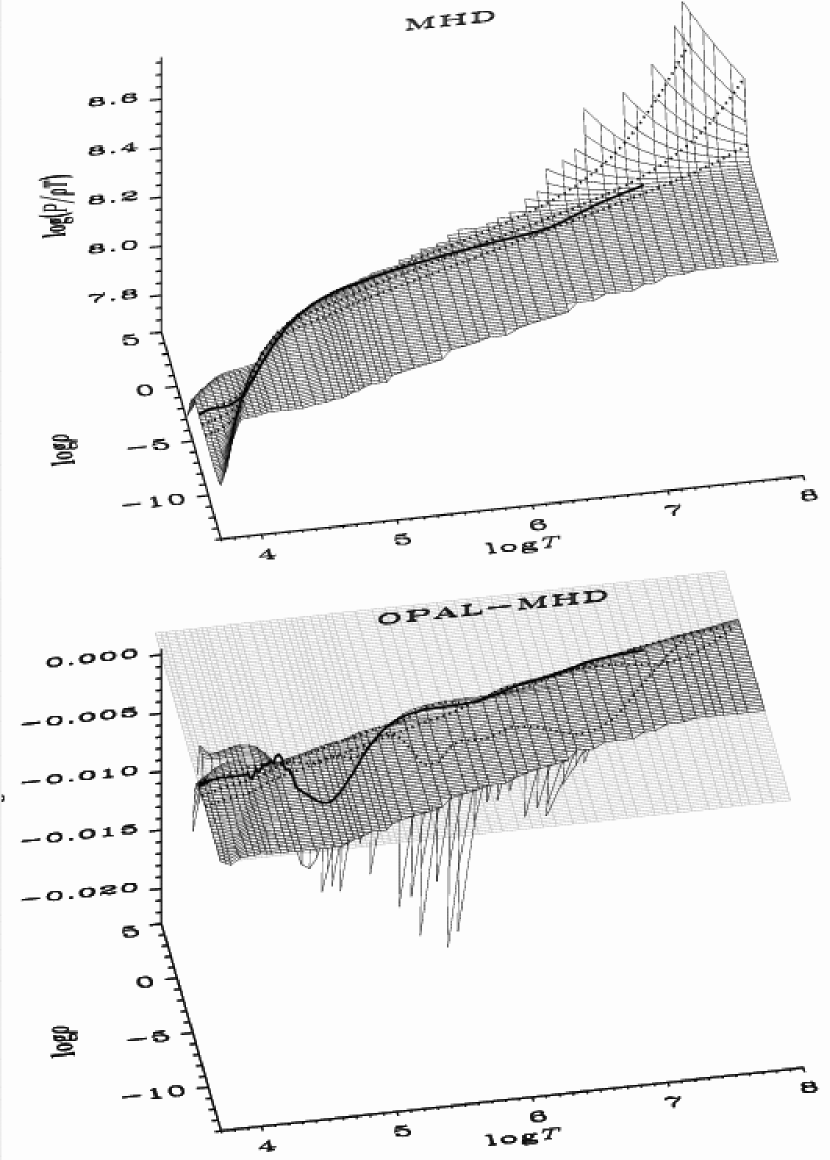
Figure 5: The reduced pressure, $P/(\varrho T)$, for the H-He mixture in the upper panel, and its differences (OPAL minus MHD) in the lower panel.

where $\mu_{ij}$ is the reduced mass. Comparing the $\tau$-function with the quantum diffraction modification in Fig. 5 of (Rogers 1994), we see a similarity in the functional form. The asymptotic behavior differs though: $\tau(x)\rightarrow x^{-1}$ for $x\rightarrow\infty$ in the hard-sphere model, whereas quantum diffraction goes as $x^{-1/2}$. The two functions are very close up to $x\simeq 1$, though, suggesting that preliminary investigations of quantum diffraction effects in the MHD EOS could be carried out by means of the $\tau$-function and a new $r_{\rm min}$ as given by Eq. (12).

Dividing Eq. (12) by $\lambda_{\rm DH}$, we find that the correction is now a function of $\varrho$ only. That is, going from a hard-sphere model of interactions, to including quantum diffraction, the factor alleviating the short-range divergence of the Coulomb potential becomes a function of $\varrho$ instead of $R$.

Abandoning the hard-sphere ion correction for the benefit of quantum diffraction, still leaves us with only the first term of the Coulomb interactions. Could the higher order terms be represented by $\tau$ in some form? It turns out that $\tau$ would only fit in a very limited range, and it would be more fruitful to use proper expressions. The present analysis however, shows that the effect of including higher-order Coulomb terms, is smaller than has previously been estimated by the MHD EOS. It therefore might be a better approximation to leave them out for at least the solar case. As shown in Fig. 13 of Nayfonov et al. (1999), the coupling parameter attains appreciable values in the outer layers of the Sun and higher-order Coulomb terms will most likely cause better agreement with helioseismology.

3 The EOS landscape in $\varrho$ and $T$

For this comparison, we have computed MHD EOS tables with exactly the same $\varrho/T$-grid points as the OPAL-tables (Rogers et al. 1996), to ensure that the equation-of-state comparison is not influenced by interpolation errors. We do actually use the respective interpolation routines to access the table-values, but by interpolating on the exact grid-points for identical mixtures, we should not lose precision in the process.

Table 1: Chemical mixtures 2 and 3 (see text)

element	$X_{i}(\%)$	[$N_{i}/N_{\rm H}$]	$X_{i}(\%)$	[$N_{i}/N_{\rm H}$]
H	80.00	0.00000	80.00	0.00000
He	20.00	-1.20098	16.00	-1.29789
C	0.00	—	0.762643	-3.09693
N	0.00	—	0.223398	-3.69693
O	0.00	—	2.171950	-2.76693
Ne	0.00	—	0.842053	-3.27923

We compare tables with three different chemical mixtures, successively adding more elements to the plasma: Mix 1 is pure hydrogen, Mix 2 a hydrogen-helium mixture and Mix 3 is a 6-element mixture that, besides hydrogen and helium, also includes C, N, O and Ne. In Table 1 we list the exact mixtures, both by mass abundance, $X_{i}$, of chemical element, $i$, and as logarithmic number fractions relative to hydrogen [$N_{i}/N_{H}$]. The choice of mixtures is that of the currently available OPAL-tables, to avoid interpolations in $X$ and $Z$. In the comparisons of this section, we have omitted the radiative contributions.

The MHD equation of state now includes relativistically degenerate electrons, (Gong et al. 2001b) as do the new version of OPAL (Rogers & Nayfonov 2002). This, of course, is significant for stellar modeling and important for helioseismic investigations of the Solar radiative zone (Elliott & Kosovichev 1998). For the present paper, however, it is irrelevant due to the lack of controversy on the subject, and we will therefore limit ourselves to dealing with non-relativistic electrons.

All plots of differences in this paper present absolute differences. Since the absolute quantities span less than an order of magnitude and as they have quite complicated behaviors, we found that normalizing the differences would confuse more than illuminate. The solar track (also presented in Sect. 4) overlaid on the surface plots is not hidden behind the surface, so as to give an idea of the behavior in otherwise obscured regions.

While the MHD tables and the pure-hydrogen OPAL table have the same resolution, Mix 2 and Mix 3 OPAL tables have three times higher resolution both in $T$ and $\varrho$. This can only affect the comparisons of the solar Mix 2 and 3 cases, Sect. 4, where it might introduce some extra interpolation-wiggles in the OPAL-MHD differences. The table comparisons are all done on the low resolution grid.

For the case of pure hydrogen (Mix 1) we plot the logarithmic absolute pressure, but for the other mixtures we plot the logarithm of a reduced pressure, $P/(\varrho T)$, to make it easier to identify non-ideal effects and the location of ionization zones. This choice will of course not affect the differences of the logarithms.

Apart from the actual pressure we also investigate the three derivatives

$$\chi_{\varrho}=\left(\frac{\partial\ln P}{\partial\ln\varrho}\right)_{T}\,,\quad\chi_{T}=\left(\frac{\partial\ln P}{\partial\ln T}\right)_{\varrho}\,,{\rm and}\quad\gamma_{1}=\left(\frac{\partial\ln P}{\partial\ln\varrho}\right)_{S}\ ,$$ (13)

where $\gamma_{1}$ is the adiabatic derivative often called $\Gamma_{1}$. These three derivatives form a complete set and fully describe the equation of state.

3.1 Pure hydrogen

We start with the simplest mixture, that is, pure hydrogen (Mix 1). The case of hydrogen is, however, far from simple, not the least because of its negative ion and molecular species. All in all five species of hydrogen: H, H⁺, H^-, H₂ and H${}^{+}_{2}$ are included in both EOS.

The number of negative hydrogen ions does never exceed a few parts in a thousand compared to the other hydrogen species. Already at moderate temperature, they dissociate into hydrogen atoms. Despite its low abundance, H^- does have an impact on the electron balance since it is the only (significant) electron sink. The heavy elements with their low abundances are most affected by this. Apart from this indirect effect on the heavy elements, the most important feature of the H^--ion is of course its bound-free and free-free opacity, which is the primary source of opacity in atmospheres of G, K and M stars.

The positive and neutral hydrogen molecules can be seen in the low-temperature-high-density corner of the tables, where their abundance reaches up to 28% of hydrogen, by mass. At slightly lower densities, which is of greater astrophysical interest, these molecules only become important at temperatures below those considered here.

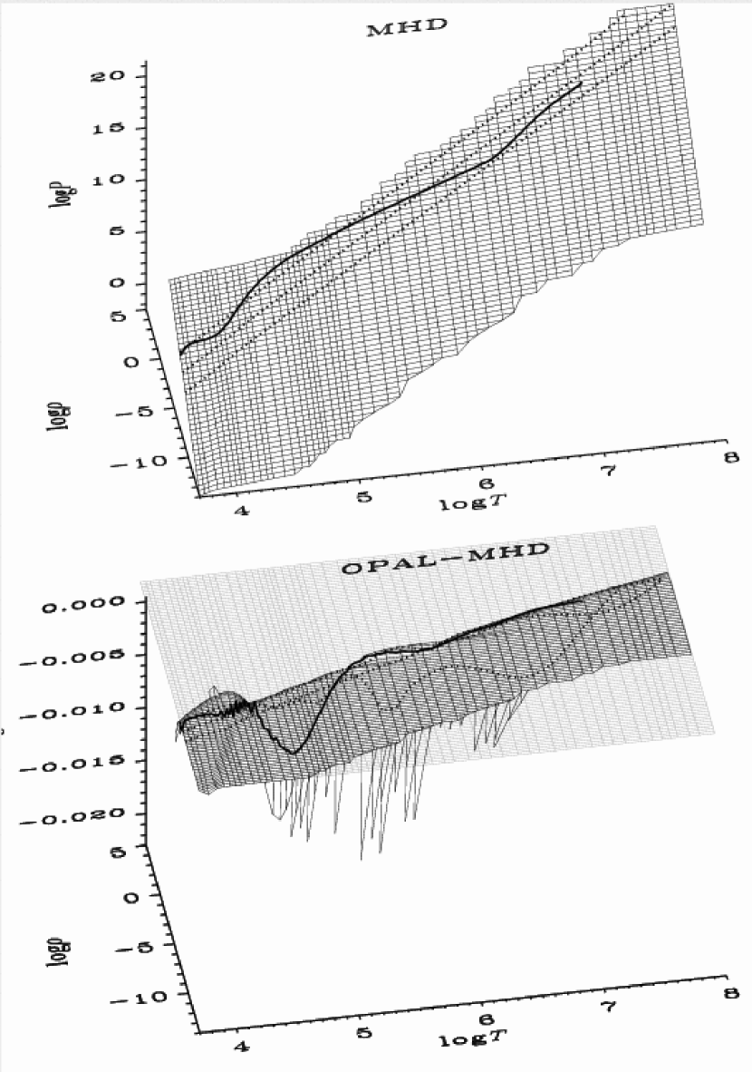
Figure 1: Comparison of log${}_{10}P$ in the two pure hydrogen tables. The upper panel shows the absolute value from the MHD EOS and the lower panel shows the difference; OPAL minus MHD. The strange boundaries of the surface simply reflects the shape of the tables. We also overlay the solar track from Sect. 4 for comparison. On this plot alone we also show iso-$R$ tracks (dotted lines) for log${}_{10}R=-2,-1,0$, going from low to high densities.

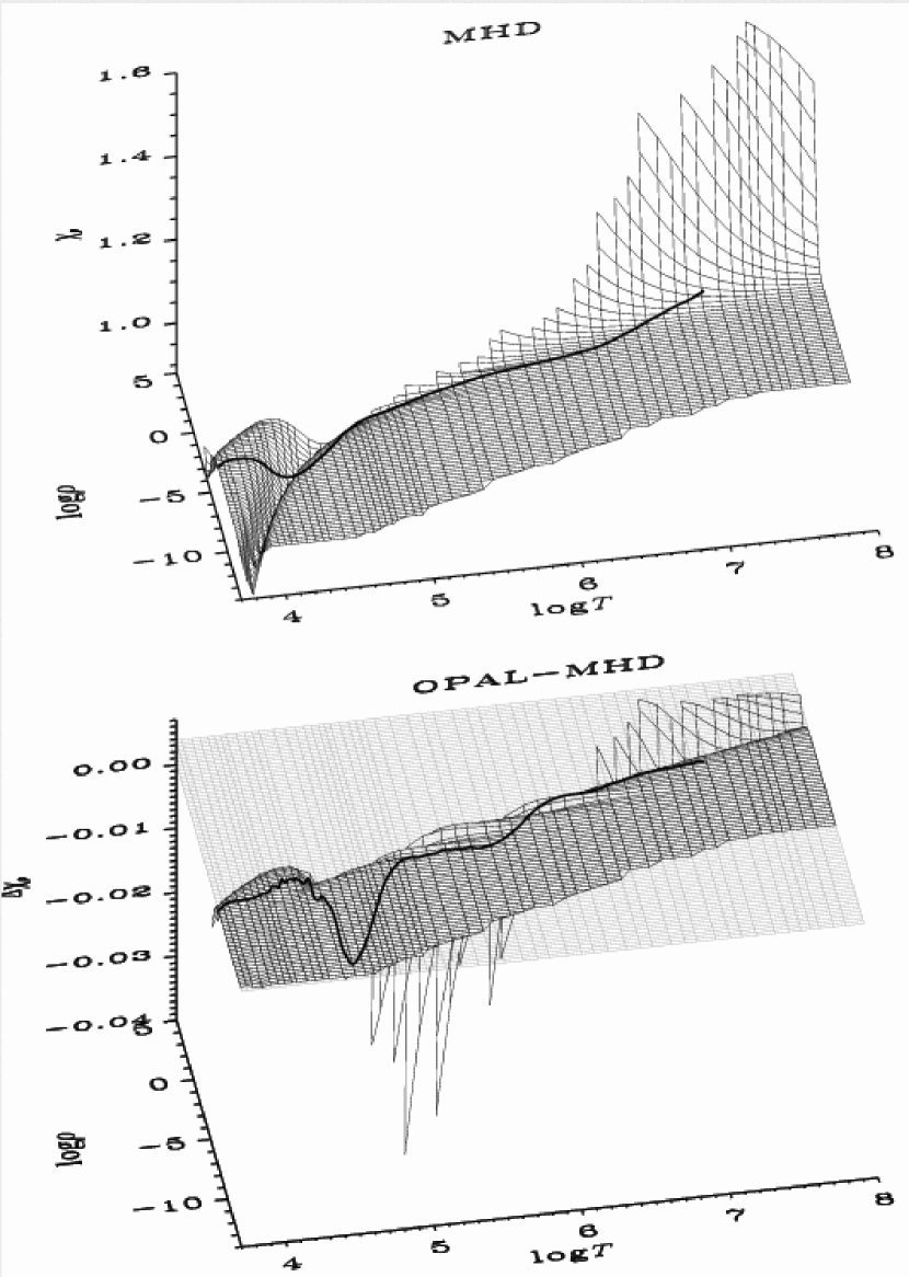
Figure 2: The logarithmic pressure derivative with respect to density $\chi_{\varrho}=(\partial\ln P/\partial\ln\varrho)_{T}$ for pure hydrogen in the upper panel, and its differences (OPAL minus MHD) in the lower panel.

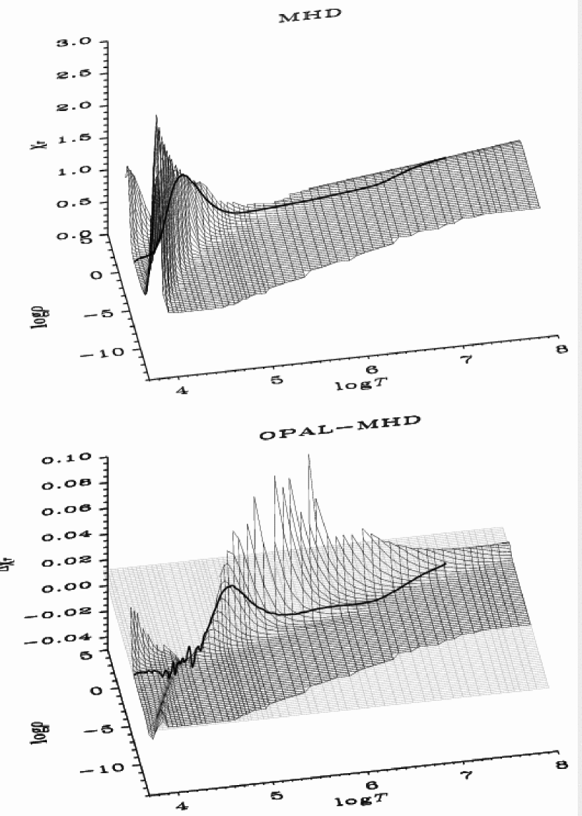
Figure 3: The logarithmic pressure derivative with respect to temperature $\chi_{T}=(\partial\ln P/\partial\ln T)_{\varrho}$ for pure hydrogen in the upper panel, and its differences (OPAL minus MHD) in the lower panel.

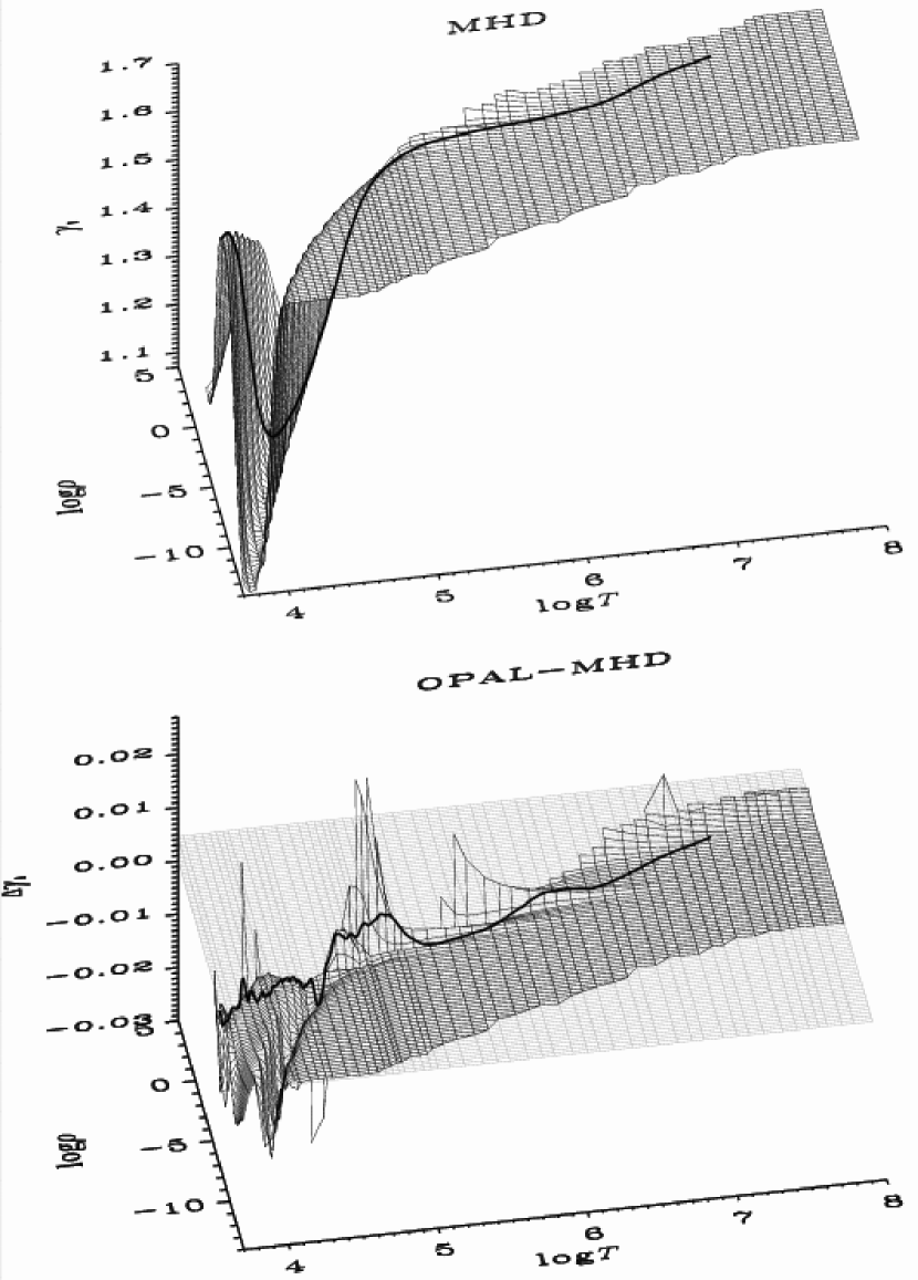
Figure 4: The adiabatic logarithmic pressure derivative with respect to density $\gamma_{1}=(\partial\ln P/\partial\ln\varrho)_{S}$ for pure hydrogen in the upper panel, and its differences (OPAL minus MHD) in the lower panel.

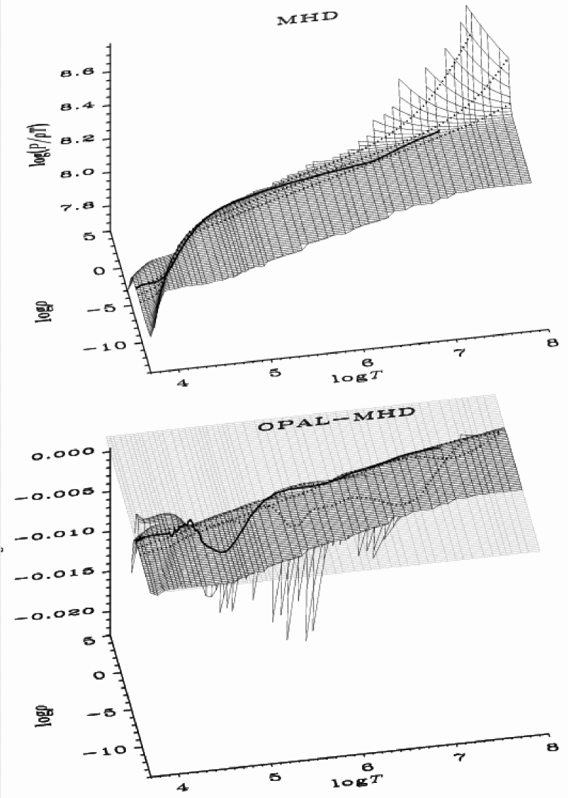
Figure 9: Reduced pressure for mixture 3 (cf. Tab. 1) in the upper panel, and its differences (OPAL minus MHD) in the lower panel.

The most important feature in the hydrogen-EOS landscapes of Figs. 1–4 is, by far, the ionization (from atom to positive ion), seen as a curved rift in all the derivatives. It is hardly visible in the surface-plot of the full pressure (Fig. 1), but becomes obvious in those of the reduced pressure (Figs. 5 and 9).

The OPAL-team introduced the quantity

$$R=T_{6}^{3}\varrho^{-1}\ ,$$ (14)

where $T_{6}=T/10^{6}$, as a convenient quantity to describe the approximate $\varrho-T$-stratification of many stars. This is clearly seen in the upper panel of Fig. 1 where we also plotted three iso-$R$ tracks, bracketing the solar track. Since the full pressure surface is so close to a plane, this plot conviniently shows the range and borders of the tabels. When interpreting the surface plots in the following sections, keep in mind this non-rectangular shape of the tables. In the lower panel of Fig. 1 these iso-$R$ tracks also bracket the main feature in the differences: A sharply rising ridge, bell-shaped in log$T$ and centered around log$T=5.5$, approximately aligned with log$R=0$. This ridge is a signature of differences in the pressure ionization. The sign of $\Delta P$ in Fig. 1 tells us that MHD has a more abrupt pressure ionization than the softer OPAL. The reason for this difference is still not completely clear. It might be related to differences in the treatment of the short-range suppression of the Coulomb forces, as mentioned in Sect. 2.2.2 and 2.2.3, or it could be a result of differences in the mechanism of pressure ionization (Iglesias & Rogers 1995; Basu et al. 1999; Gong et al. 2001a).

We now turn to the logarithmic pressure derivatives, $\chi_{\varrho}$ and $\chi_{T}$, displayed in Fig. 2 and 3, respectively. In both figures, the ionization zone is easily recognized as the canyon or ridge starting in the low-temperature-low-density corner, slowly bending over to follow the solar track and disappear at about log$T=6$.

In most of the $\varrho-T$ plane both derivatives are equal to one reflecting that the gas is a perfect gas. In this region the differences are very small (i.e. less than 0.03%), confirming that both the chemical and the physical picture converges appropriately to the perfect gas case.

At low temperatures $\chi_{\varrho}$ and $\chi_{T}$ are dominated by temperature ionization, which is about an order of magnitude more prominent in $\chi_{T}$ than in $\chi_{\varrho}$. This region is a fairly well known regime and here we can directly compare the two pictures. The differences are indeed small in this region, less than 1% and less than a tenth of the differences in the high-$R$ ridge.

The rise of $\chi_{T}$ in the low-$T$-high-$\varrho$ corner is due to H₂-molecules. About 28% by mass, of the hydrogen atoms are bound in molecules in this region, but at higher densities they quickly dissociate. As beautifully illustrated by Mihalas et al. (1988) in their Fig. 1, hydrogen recombines fully to H₂ at large densities when assuming a Saha equilibrium. This is obviously absurd (there is no room for molecules – or atoms) and both the MHD and OPAL EOS pressure dissociate hydrogen here, as would be expected from a realistic EOS. In MHD this is modeled in the same manner as the pressure ionization of atoms, as explained below Eq. (2). This is most likely a rough approximation, but due to the efficient ionization with density, the details might be less important. The fact that the differences increase while the absolute value decreases indicates that MHD is pressure dissociating faster than OPAL.

The differences are again dominated by the sharp ridge at high $R$, but in contrast to pressure (Fig. 1), the differences in $\chi_{\varrho}$ and $\chi_{T}$ return to zero for high temperatures and densities. As for pressure, the solar track falls over or climbs the $R$-edge in the middle of the ionization zone, as it is traversing the iso-$R$ at log$R\simeq 0$.

These high-$R$ differences occur in a region where there is competition between the Coulomb terms and electron degeneracy. This makes the interpretation much more difficult. Two possible reasons are the previously mentioned short-range part of the Coulomb interactions and the changes induced in the internal atomic states by the dense, perturbing surroundings.

In the MHD EOS, all energy levels of internal states are assumed to be unaltered by the plasma environment. That is, the effect of the perturbation by surrounding neutral and charged particles on the internal state is restricted to a lowering of the occupation probability of the given state only. In the OPAL EOS, the net result looks similar, but there the relative stability of energy levels to perturbations is not merely postulated but the result of in-situ calculations of the Schrödinger or Dirac equation for each configuration of nuclei and electrons, based on parameterized Yukawa potentials (Rogers 1981b), as mentioned in Sect. 2.1.2.

Looking at $\gamma_{1}$ in Fig. 4 we immediately notice how well this quantity displays the ionization zones while leaving out everything else. This property is also reflected in the differences, which here are of about the same magnitude in the ionization zone as in the high-$R$ ridge. The high-$R$ differences have also changed characteristics, changing sign periodically, while retaining the overall bell-shape in log$T$ of the amplitude. We mention, however, that at least some of this behavior might be due to the numerical differentiation scheme used in the OPAL EOS (see Sect. 5 and Fig. 26).

3.2 Hydrogen and helium mixture

The effect of helium in the thermodynamical quantities is revealed by the addition of 20% helium and comparison with the pure-hydrogen case. The first thing we notice from Fig. 5 is how well the reduced pressure $P/(\varrho T)$ reveals all the dissociation and ionization zones (except H^-); The H₂-formation in the low-$T$-high-$\varrho$ corner and the prominent ionization of hydrogen together with the two He ionization zones, the first eventually merging with the H ionization. The effect of degenerate electrons is evident in the high-$T$-high-$\varrho$ corner.

We also notice another thing: while the pure hydrogen OPAL-table was cutting the high-$\varrho$, low-$T$ corner, leaving a little less for the comparison, the mixture OPAL-tables allow a full comparison since they have the same boundaries as the MHD tables. The slightly larger table reveals a new feature in the differences. For pure hydrogen, the pressure difference drops suddenly in the high-$\varrho$, low-$T$ corner, due to faster molecule formation in OPAL as compared to MHD. But in the slightly larger tables used for the remainder of this section, this difference suddenly goes to zero before it falls down the high-$R$ edge.

In the pressure differences, one can just barely identify the first helium ionization zone, whereas the second is too faint to be seen here. The high-$R$ differences are a little smaller than for pure hydrogen, as anticipated from Eq. (8) and the discussion following it. This can be most clearly seen by comparing the dip in the hydrogen ionization zone.

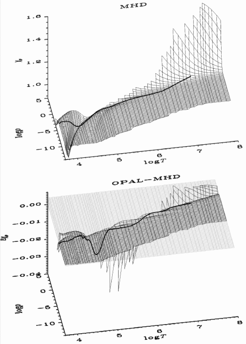
Figure 6: $\chi_{\varrho}$, the logarithmic pressure derivative at constant temperature, for the H-He mixture in the upper panel, and its differences (OPAL minus MHD) in the lower panel.

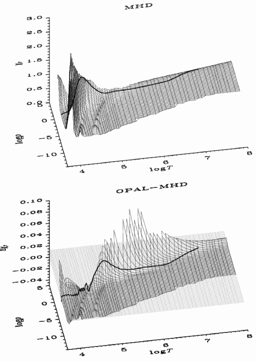
Figure 7: $\chi_{T}$, the logarithmic pressure derivative at constant density, for the H-He mixture in the upper panel, and its differences (OPAL minus MHD) in the lower panel.

The addition of helium is also evident in the logarithmic pressure derivatives in Fig. 6 and 7. First we see the deep rift (ridges in Fig. 7) of the hydrogen ionization zone. Then comes a small groove from the first helium ionization zone, a groove which, when it widens and gets shallower at higher densities, eventually merges with the hydrogen ionization zone, as is the case for the solar track. Widely separated from the hydrogen and first helium ionization zones, we find the second helium ionization zone. It seems to disappear at the low density edge of the table, but that is only so because the ridge gets very sharp and is unresolved in temperature, at low densities. Hotter stars, that is, stars shifted towards lower $R$, will clearly exhibit three, more distinct ionization zones when compared with the Sun.

Apart from the two helium ionization zones, the differences in the pressure derivatives are very similar to the pure hydrogen case. The high-$R$ differences are somewhat smaller though, as are the differences in the hydrogen ionization zone. The differences in $\chi_{\varrho}$ also displays a very small ripple along log$R\simeq-4$, which might be due to differences in the differentiation technique (see Sect. 5).

From the differences in $\chi_{T}$ (Fig. 7), we see that the absolute differences in the three ionization zones are just about the same. If we instead compare the differences relative to the size of the respective ionization ridges, we get 0.16% and 3% relative differences for the hydrogen and helium ionization zones respectively. That is, MHD and OPAL have about 20 times better agreement on hydrogen than on helium.

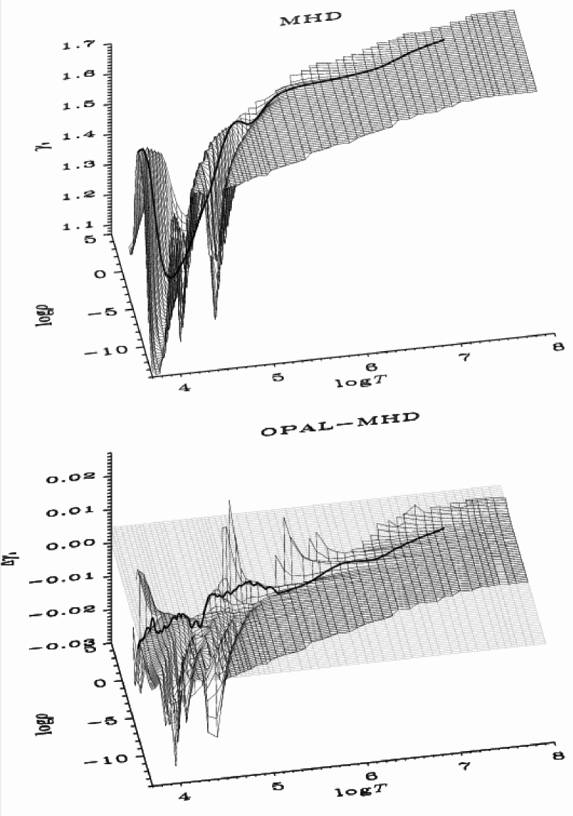
Figure 8: $\gamma_{1}$ for the H-He mixture in the upper panel, and its differences (OPAL minus MHD) in the lower panel.

In Fig. 8, $\gamma_{1}$ appears like what we would anticipate from the pure hydrogen case in Fig. 4. The first helium ionization zone is only visible at low densities, as it merges with the hydrogen ionization zone shortly before the solar track is reached.

The differences, however, exhibit a much more complicated structure. Along each of the ionization zones, there is a deep valley in the differences, and along the bottom of these valleys runs a very sharp ridge, bringing the differences up to positive values. This is a clear sign of a broad negative peak minus a sharp negative peak, meaning that MHD temperature ionize faster than does OPAL. In the beginning of this section, we found that MHD was also pressure ionizing faster than OPAL, so all in all OPAL is the softer EOS of the two. The ridge-in-the-middle-of-the-valley picture is also found in the pure hydrogen case (Fig. 4), but as the hydrogen ionization zone is not fully covered at low densities, the low-$T$ side of the valley is missing.

3.3 H,He,C,N,O and Ne mixture

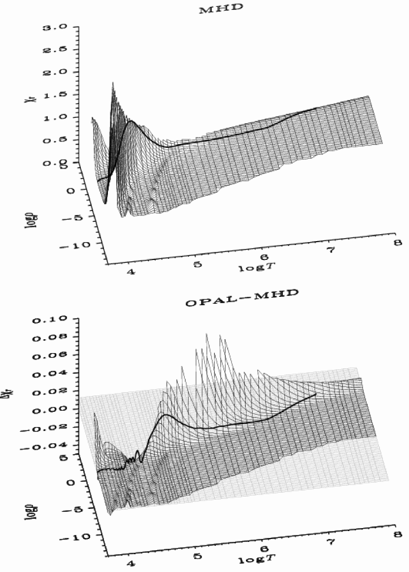
Figure 11: $\chi_{T}$, the logarithmic pressure derivative with respect to temperature, for the full mixture in the upper panel, and its differences (OPAL minus MHD) in the lower panel.

In this section we add the last four elements considered, namely carbon, nitrogen, oxygen and neon. Comparing Figs. 9-11 of this section with the corresponding Figs. 5-7 of the previous section, hardly any differences appear, neither in the absolute values nor in the differences between the two EOS.

For a few points on the high-$R$ boundary of the tables, differences in $\chi_{\varrho}$ and $\gamma_{1}$ have increased dramatically. At least some of these odd points are the same for $\chi_{\varrho}$ and $\gamma_{1}$. This might indicate that these points are spurious, possibly associated with convergence problems in either EOS in this difficult region.

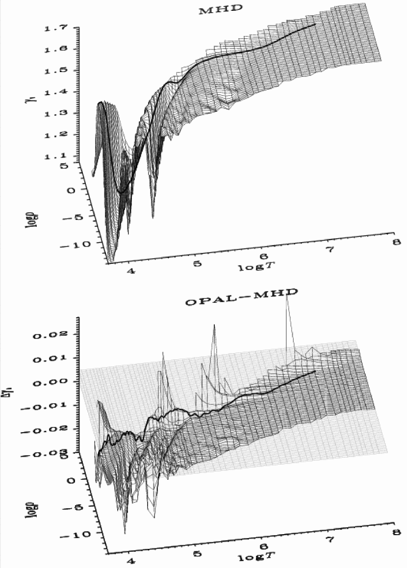
Figure 12: The adiabatic logarithmic pressure derivative, $\gamma_{1}$, for the six element mixture in the upper panel, and its differences (OPAL minus MHD) in the lower panel.

The heavy elements are just barely discernible in the differences of $\chi_{\varrho}$ (Fig. 11). However, for $\gamma_{1}$, in Fig. 12, the heavy elements appear clearly both in the absolute $\gamma_{1}$ and in the $\gamma_{1}$ differences, especially along the low-$\varrho$ edge of the table. Between the first and second ionization zones of helium (cf. Fig. 8), we notice some wiggles, which are likely resulting from the third ionization zones of carbon and nitrogen, and the second ionization zones of oxygen and neon. Above the second ionization zone of helium, we can see all the ionization zones from the fourth ionization zone of carbon right up to the tenth ionization of neon, although they are not all resolved in this $\varrho$-$T$-grid. A rough estimate reveals that the relative difference between MHD and OPAL for the heavy elements is of about the same magnitude as the one for the helium ionization zones, i.e. 3%, or about 20 times worse than the 0.16% agreement for hydrogen.

This unexpectedly large discrepancy for the heavy elements might be a hint that these differences are primarily caused by differences in the lower excited states. For hydrogenic ions, there are analytical solutions for all states. This might explain the small discrepancy for hydrogen. For ions with more than one electron there are no analytical treatments, except for their higher states, which become nearly hydrogenic. So it might well be that the lower lying states of the non-hydrogenic ions are responsible for the differences noticed here. The Yukawa potentials (Rogers 1981b), which are used to describe bound electron states in OPAL, are fitted to give the correct (experimental) ionization energies. MHD uses experimental results for the energy levels. It is no surprise therefore to get quasi-perfect agreement on the location of the ionization zones (confirmed by the ridge-in-the-middle-of-the-valley picture in the $\gamma_{1}$ differences), whereas the energies of lower lying excitation levels might differ These differences propagate into the partition functions and affect the course of ionization. In addition, the differences in the adopted micro-field distribution, and the mechanism by which they ionize highly excited states, might play a rôle in this region (Nayfonov & Däppen 1998; Nayfonov et al. 1999). Since the differences occur at the low-$\varrho$ edge of the table, we expect however, that they mainly reveal differences in the thermal ionization, not in pressure ionization.

Let us return to pressure and have a closer look at the non-ideal effects in the high-$T$-high-$\varrho$ corner. From the dotted iso-$R$ lines in Fig. 9, it is clear that the non-ideal effects are not functions of $R$ alone. Instead it turns out that they are largely functions of $\varrho^{2}/T^{3}$. Comparing the perfect gas pressure and the fully degenerate, non-relativistic electron pressure

$$P_{\rm perf}=\frac{\varrho k_{\rm B}T}{\mu m_{\rm u}}\quad{\rm and}\quad P_{\rm e}^{\rm deg}=\frac{1}{5}\left(\frac{3}{8\pi}\right)^{2/3}\frac{h^{2}}{m_{\rm e}}\left(\frac{\varrho}{\mu_{\rm e}m_{\rm u}}\right)^{5/3},$$

we see that the two pressures compete along $\varrho^{2}\propto T^{3}$-lines. This means that relative to high-$R$ (Coulomb) effects, there are more degeneracy effects in the high-$T$-$\varrho$ corner of the table, which reveals the nature of the sharp rise of both $P$ and $\chi_{\varrho}$ in this region. The correlation with larger OPAL$-$MHD differences (See lower panel of Fig. 9) prompted us to perform a direct comparison between the Fermi-Dirac integrals from the two codes. We found non-systematic differences a reassuring eight orders of magnitude smaller than the EOS differences we observe in this region.

An alternative explanation could be the lack of electron exchange effects in the MHD EOS. This is a combined effect of Heisenberg’s uncertainty relation (Heisenberg 1927) and Pauli’s exclusion principle (Pauli 1925): Due to the former, electron wavefunctions are extended, but due to the latter, the wavefunctions of two close electrons with same spin cannot overlap. This results in the combined wavefunction either having a bulge or a node at the mid-point between the two electrons, giving rise to two different kinds of contributions to the Coulomb interactions. In the fully ionized, weak degeneracy limit, the first-order e-e exchange pressure (DeWitt 1961, 1969) is negative and proportional to $\varrho^{2}/T$. Analyzing the differences in solar solar case, we actually find in Sect. 4, that those powers of $\varrho$ and $T$ are the ones best describing the differences above $T\simeq 2\times 10^{6}\,$K

4 Comparisons in the Sun

To study the EOS under solar conditions, we have evaluated the MHD and OPAL EOS on a $\varrho-T$ track that corresponds to the Sun using the respective interpolation routines. Obviously, this is a simplified comparison, not of evolutionary models of the Sun, but merely of the equations of state for fixed solar-like circumstances. As demonstrated elsewhere, such a simplified procedure is well justified (See e.g. Christensen-Dalsgaard et al. 1988).

We use the three chemical mixtures from Table 1, bearing in mind that Mix 3 has about twice solar metallicity. In contrast to the comparisons of the previous section, we now include radiative contributions. This will of course not change the differences of thermodynamic quantities, since both formalism use the well-known additive radiative contributions (Cox & Guili 1968).

In all the figures of this section, we notice that the MHD and the OPAL EOS differs very little at temperatures below 20 000 K and above $10^{6}$ K, but they differ significantly in between. And though the differences are small above 20 000 K, they are still of the same magnitude as the relativistic effects which are well within reach of helioseismology (Elliott & Kosovichev 1998) —and they look intriguingly systematic.

The wiggles in the differences, most noticeable in the region between log$T$=4-4.5, are almost certainly due to the interpolation schemes. They become quite dominant in the $\gamma_{1}$ difference. As mentioned in Sect. 3, the tabular resolution of the OPAL tables for Mix 2 and 3 is about three times better than that of the corresponding MHD tables, whereas the pure hydrogen tables (Mix 1) have the same (low) resolution. Comparing the figures based on low resolution tables (figs. 13–16) with those based on high resolution table (Figs. 17–20), we notice that the high-frequency component in the difference plots are much larger in the former than in the latter. This is especially visible around $\log T\simeq 4--4.5$ and $\log T\simeq 5.1--5.9$. This indicates that the OPAL results have larger interpolation errors, since the MHD tables all have the same resolution. A more detailed study of interpolation errors in tables, was written by Bahcall et al. (2004), for the case of OPAL opacities.

4.1 Pure hydrogen

If we take a look at the absolute pressure in Fig. 13 a), we notice a bend at log$T=6.4$. This marks the bottom of the convection zone. Inside the convection zone, that is below log$T=6.4$, there is adiabatic stratification of pressure and temperature, i.e.

$$\nabla_{\rm ad}=\left(\frac{\partial\log T}{\partial\log P}\right)_{\rm ad}=\frac{\gamma_{1}-\chi_{\varrho}}{\gamma_{1}\chi_{T}}.$$ (15)

When the gas is nearly fully ionized, essentially $\nabla_{\rm ad}=2/5$, evidenced as the straight-line part of the curve in Fig. 13 a). In the ionization zones (the outer $0.02R_{\odot}$), $\nabla_{\rm ad}$ is lowered to about 0.11 at log$T\simeq 4.1$, again clearly evidenced as a depression in the pressure curve. $\nabla_{\rm ad}$ comes back to $2/5$ at log$T\simeq 3.76$, but this happens at the top of the convection zone where there is a downward bend to a radiative stratification. The depth of the convection zone is about 0.285$R_{\odot}$, and just slightly higher, at a depth of 0.25$R_{\odot}$, hydrogen finally gets fully ionized according to MHD (fewer than 1 in 10⁵ are still neutral), at a temperature of log$T=6.3$. For comparison, MHD predicts that hydrogen is 99.88% ionized in the middle of the convection zone at log$T=6$. Both results are largely due to pressure ionization, without which about a quarter of the hydrogen would still be neutral at the solar center. So, although it is reasonable to say that the hydrogen ionization zone is confined to the outermost 2% of the Sun, one should also bear in mind the long tail of unionized hydrogen that is extending almost to the bottom of the convection zone. This tail has an especially large effect on the opacity, since in the visual and UV only bound states can add opacity to the constant “background opacity” from electron scattering.

In the upper plot of Fig. 14 we can actually see the differences between the absolute values of $\chi_{\varrho}$. It is evident that OPAL has a much smoother and broader ionization zone than the somewhat bumpy MHD. Turning off the $\tau$-correction (dashed lines), almost centers MHD on OPAL, but the bumps remain the same. These bumps were also noticed by Nayfonov & Däppen (1998) and their analysis showed that in the region where log$T=4.2$–$5.2$ the bumps are caused by excited states in hydrogen. In this part of the Sun, hydrogen is 30% increasing to 97.8% ionized, so even a small amount of neutral hydrogen can have a significant effect on the EOS.

At log$T\gtrsim 6.5$ we see how degeneracy sets in, with the electron component of $\chi_{\varrho}$ increasing towards its fully degenerate value of $5/3$. In the lower plot, we notice that degeneracy is accompanied by an increase in the differences. This could be attributed to the MHD EOS not including electron-electron exchange effects, as pointed out in Sect. 3.3.

The behavior of $\chi_{T}$ (Fig. 15) confirms the picture obtained from Fig. 14, that is, MHD ionizing faster and being more bumpy than OPAL. However, since the dynamic range of $\chi_{T}$ is much larger than that of $\chi_{\varrho}$, the bumps, which have still about the same size as those of $\chi_{\varrho}$, are now being dwarfed by the much larger ionization peak in $\chi_{T}$. Comparing the differences shown in the lower plots, we notice that the overall differences are about twice as large as for $\chi_{\varrho}$, but the ionization peak in the respective upper plots is about 10 times larger for $\chi_{T}$ than for $\chi_{\varrho}$. We also notice that in $\chi_{T}$, as a likely result of the higher dynamic range, the interpolation-wiggles at log$T\lesssim 4.6$, are much more prominent than in $\chi_{\varrho}$.

We can also distinguish MHD from OPAL in the absolute values of $\gamma_{1}$ (Fig. 16 a)), although they are much closer than in the $\chi$’s of Fig. 14 and 15. This is confirmed in the differences shown in panel b), which are overall smaller by an order of magnitude compared to the $P$-, $\chi_{\varrho}$- and $\chi_{T}$-differences. In contrast to our experience with $P$, $\chi_{\varrho}$ and $\chi_{T}$, here diminishing the $\tau$-correction in MHD (dashed and dotted lines) does not lead to any better agreement with OPAL. This is again convincing evidence that $\gamma_{1}$ is a very efficient filter for high-$R$ effects. The differences that we see are therefore due to the physics of ionization, except at low temperatures, where interpolation errors seem to dominate.

4.2 Hydrogen and helium mixture

The effect of helium is very hard to see in the reduced pressure shown in Fig. 17 a), and in the shape of the differences in Fig. 17 b). However, a comparison with the pure hydrogen case (Fig. 13), allows us none the less to see a few changes to the differences in the lower panels; The peak around log$T=4.7$ gets considerable smaller by adding helium, except for the $\tau=1$ case, where the difference actually increases in this region. Also, the differences outside the high-$R$ region decrease by adding helium, independently of the choice of $\tau$.

In general, adding helium does not alter the shape of the differences in $P$, $\chi_{\varrho}$ or $\chi_{T}$, and the changes due to composition are only manifest by a change of the amplitude of the peak around log$T=4.7$. This is surely due to the fact that most of the ionization in the Sun takes place in the high-$R$ region, so that the first-order high-$R$ differences due to the ionizations themselves simply dwarf the second-order effects due to detailed partition functions, among other. The solar track does follow the ionization zones to some degree, and only enters the hydrogen ionization zone “head on”. With the solar track curving along the hydrogen ionization zone in this way the ionization features will be smoothed out over a much larger temperature interval than if we had examined an iso-chore. This smoothing leads to more blending of ionization zones from various elements, hampering analysis. The shape, merging and smoothing of the ionization features is best seen in Figs. 9–11.

This behavior is clearly illustrated in, e.g., $\chi_{\varrho}$ (Fig. 18 a), where we observe a rather sharp onset of ionization followed by a much slower transition to full ionization. The second ionization of helium appears as part of the bump around log$T=5$. The bump is somewhat more pronounced than in the pure hydrogen case. A more careful comparison with the pure hydrogen case (Fig. 14) reveals the first ionization zone of helium as a slight extension of the hydrogen peak, on the side towards higher temperatures. Helium gets almost fully ionized at log$T=6.0$, where 1.77% is singly ionized and 98.23% doubly ionized. The ionization only proceeds gradually towards higher temperature, until at log$T=6.75$ it suddenly becomes fully ionized. This happens at a depth of $0.63R_{\odot}$, at the edge of the hydrogen burning core. At log$T=6.5$, just slightly above the temperature where hydrogen gets fully ionized, there is finally no more neutral helium left.

For $\chi_{T}$ (Fig. 19 panel a), the bump at log$T\simeq 5$ is a clear sign of the helium added, as opposed to the similar but more entangled bump in $\chi_{\varrho}$ (cf. Fig. 14 and 18). The second He ionization zone is very distinct in $\gamma_{1}$ (Fig. 20 a), and the first ionization zone is manifested by a widening of the hydrogen ionization zone towards the high-$T$ side. The differences (panel b) are just as entangled as for pure hydrogen (Fig. 16) but with lower amplitude. On the descending part, just above log$T=5$, there are some large interpolation errors, caused by the change to the coarser grid. We also notice a peculiar bump at log$T=6.6$

Looking at the various difference plots in this section, we see a correlation between a high amplitude in the differences and a high $R$-value, a property we already inferred from the solar track (Fig. 1). The minimum in $R$ is found at the base of the convection zone, where we also find a local minimum in the magnitude of the differences between the EOS. The location of this local minimum coincide for all four thermodynamic quantities. This confirms our suspicion that at least some of the discrepancy stems from $\tau$. The reason for this conjecture is that the differences between MHD EOS with different $\tau$ almost vanishes in this region, whereas they increase in the same way as the MHD-OPAL differences grow for intermediate temperatures.

At high temperatures, above a minimum occurring at log$T\simeq 6.4$, the MHD-OPAL differences grow, but the differences between the three $\tau$ versions themselves remain small. On the solar track, log$R=-1.8$ at the minimum of the MHD-OPAL difference, and it only rises slightly to -1.4 at log$T=6.8$ where the solar track bends to follow more or less an iso-$R$ line. The constant $R$ value is attained around log$T=6.15$. The differences between the $\tau$-versions are indeed the same in both of these regions (this is best seen in the pressure differences e.g. Fig. 17), which explains why the three curves with different $\tau$ follow each other so closely at high temperatures. The MHD-OPAL difference in this region can therefore not be explained by the $\tau$-correction. It also turns out that in this region, the differences of the $\varrho$-$T$ plane are mainly functions of $\varrho^{2}/T^{3}$ instead of $R$. In Sect. 3.3 we suggested that this dependence might arise from electron exchange effects or maybe from possibly different evaluations of the Fermi-Dirac integrals. However, a third explanation might be based on the quantum diffraction mentioned in Sect. 2.2.3.

4.3 H,He,C,N,O and Ne mixture

Adding C, N, O and Ne to the H-He mixture has two main effects: first, it displaces 4% He (cf. Tab. 1), thereby diminishing the helium features, and second it leads to a slight decrease in the high-$R$ OPAL-MHD differences due to the increased mean charge [see Eq. (8)]. Only in $\gamma_{1}$ (Fig. 24), can the heavy elements be observed directly. Comparing with the H-He case (Fig. 20), and going from low to high temperatures, we first notice a slight diminishment of the feature associated with the first ionization zone of helium due to the 4% decrease of the helium content. This weakening of the He⁺ feature is counteracted by the second ionization zone of carbon (24.38 eV), as well as that of the less abundant Ne (21.56 eV) and N⁺ (29.60 eV). The feature of the second ionization zone of helium (54.42 eV) is also diminished, but counteracted by the third ionization zone of oxygen O⁺⁺ (54.93 eV), the most abundant heavy element. C⁺⁺, C³⁺, N⁺⁺ and Ne⁺⁺ adds further ionization in this temperature region, but on either side of of the helium bump, effectively smoothing the feature a little.

This feature is used for helioseismic determinations of the Solar helium abundance (Basu & Antia 1995), as there are no helium lines in the Solar (photospheric) spectrum. A change in the strength of this feature, either from a change in abundances (primarily oxygen) or a change in the equation of state, will therefore have an effect on the Solar helium abundance. This is in particular interesting as the proposed new Solar abundances by Asplund et al. (2005) lowers $Z$ to about 1.1% and it will be discussed further in Sect. 6.

The helium signal in $\gamma_{1}$ is also shown as the solid curve in Fig. 25 where we have plotted the differences between Mix 2 and Mix 3 with respect to Mix 1. The two helium ionizations zones are prominent at $\log T\simeq 4.6$ and at $\log T\simeq 5$. There are also effects from the 20% lower hydrogen abundance, especially at lower $T$. The dashed line in Fig. 25 shows the effect of adding the metals; reducing the helium features, adding a broad feature around $\log T\simeq 6.2$ and adding a “continuum” of features from there, and down to the second helium ionization zone. Note that the helium features are not reduced in proportion to the change in $Y$, indicating the metals that have ionization zones here.

Continuing in our exploration of $\gamma_{1}$ and going to higher temperatures we notice a slight straightening of the “knee” around log$T\simeq 5.3$, due to the intermediate ionization stages of C, N and Ne with ionization potentials between 47 eV and 240 eV. Finally, at log$T\simeq 6.2$, we find a broad dip supplied by the two uppermost ionization stages of C,N,O and Ne, having ionization energies in the range between 400 eV and 1 360 eV.

The only quantity in which the introduction of heavy elements is manifested directly is $\gamma_{1}$, which is an important key variable in helioseismology (since it is closely related to adiabatic sound speed $c^{2}=\gamma_{1}p/\varrho$). The promise of these features is that the presence of heavy elements is well marked in $\gamma_{1}$. Actually, this marking is so distinct (Gong et al. 2001a), that in future solar and stellar applications of the MHD and OPAL equations of state it might be worth to include more heavy elements The influence due to our small quantity of heavy elements is about three times larger than the difference between OPAL and MHD, though we hasten to add that our heavy element abundance of $Z=4\%$ is chosen too high in order to exhibit the effects more clearly; they would of course decrease with a more solar metallicity around $Z=1$–$2$%.

We have not discussed radiation pressure yet, merely because of the lack of controversy about it. However, it is worth a few notes. The ratio between radiation pressure and gas pressure is constant along iso-$R$ lines the two being equal around log$R\simeq-4.5$. The largest radiation effects therefore occur at log$T=6.4$ where there is also the smallest discrepancy between OPAL and MHD. The effect of radiation changes log$P$, $\chi_{\varrho}$, $\chi_{T}$ and $\gamma_{1}$ by $0.0007,-0.001,0.003,-0.002$, respectively.

5 Discrepancies due to differentiation

A closer inspection of the derivatives in the perfect gas region reveals some discrepancies which are likely due to the numerical differentiation performed in the OPAL EOS. This is most noticeable in $\gamma_{1}$, where the OPAL-MHD differences in the perfect gas region are as large as 0.03%, which admittedly is small indeed. Helioseismology will, however, soon be dealing with such precision. This difference most probably comes from problems in the numerical calculation of an adiabatic change as performed in OPAL (note that MHD uses essentially analytical expressions for $\gamma_{1}$, $\chi_{\varrho}$ and $\chi_{T}$ Since an adiabatic change is not rectangular in the $T-\varrho$ plane, such an interpretation is consistent with the fact that the differences in the derivatives with respect to $\varrho$ and $T$ ($\chi_{\varrho}$ and $\chi_{T}$, respectively) are about one order of magnitude smaller. This also means, that in the ionization zones where pressure and entropy are non-linear functions of $\varrho$ and $T$, this differentiation noise must be much larger. On the other hand, the differences between OPAL and MHD are still at least an order of magnitude larger than this differentiation noise. We hope, however, that future improvements will make OPAL and MHD converge to within that level of the actual EOS, requiring higher numerical standards.

The differences in $\chi_{\varrho}$ and $\chi_{T}$ have a tendency to follow iso-$R$ tracks, while the differences in $\gamma_{1}$ follow isotherms. These two behaviors are still unexplained. In Fig. 26, the differences following isotherms are pretty clear, but the iso-$R$ differences are also visible, well below the rising mountain at high $R$-values.

6 New metal abundances

Recently the previously converging Solar abundances (Grevesse & Noels 1993; Grevesse et al. 1996), have been upset by new abundance analysis by Asplund et al. (2005) (and references therein) performed on 3D radiation-coupled hydrodynamical simulations of convection in the Solar surface layers (See, e.g., Stein & Nordlund 1998). This approach completely avoids the concepts of micro- and macro-turbulence of 1D models, as the line-broadening velocity-fields are included explicitly. This results in synthetic spectral lines that not only have the widths of the observed lines, but also match the detailed (asymmetric) shapes of the lines (Asplund et al. 2000). This reduces the number of free parameters to essentially the abundances we seek, and gives less ambiguous abundances. The result is a general lowering of the Solar heavy element abundances (Asplund et al. 2005) and most notably a halving of the oxygen abundance. This has a severe impact on the previously close agreement between Solar models and helioseismic observations (See, e.g., Bahcall et al. 2005a, and references therein). The lowering $Z$ to about 1.1%, decreases the opacity at the bottom of the convection zone thereby decreasing the depth of the convection zone (Bahcall et al. 2005a, b) at odds with helioseismic measurements (Christensen-Dalsgaard et al. 1991; Basu & Antia 1997; Bahcall et al. 2004).

In Sect. 4.3 we touched upon the determination of the helium abundance by helioseismically measuring the bump in $\gamma_{1}$ around $T=10^{5}\,K$. This bump also has a contribution from oxygen, as shown in Fig. 25, and a lowering of the oxygen abundance will therefore have an effect on the Solar helium abundance. To keep the agreement with the helioseismic helium abundance determination, a smaller $Z$ has to be accompanied by a an increase in $Y$. We have interpolated the $\gamma_{1}$-differences of Mix 2 and 3 with respect to Mix 1, to find the amplitude of the feature around $\log T=5$. From this we find that a change of $Z$ from 1.8% to 1.1% should be accompanied by an increase of $Y$ by 0.0039 (using MHD) in order to keep the bump unchanged. Basu & Antia (2004) perform a helio-seismic determination of the Solar helium abundance using the new and lower $Z$, but based on the updated OPAL EOS (Rogers & Nayfonov 2002). They use a slightly higher $Z=1.26$% for the new abundances and find an increase in $Y$ of 0.0050. To translate to our choices of $Z$ we derive a $\Delta Y/\Delta Z=-1.029$ from their results, which gives a $Y$-increase of 0.0072. This means that the $\gamma_{1}$ of the OPAL EOS is about 1.8 times more sensitive to the heavy element content, than the MHD EOS is. Evolutionary models with the two sets of abundances, calibrated to the present Solar radius and luminosity, on the other hand, result in a decrease of $Y$ by 0.005 (Bahcall et al. 2005a)—a total discrepancy between models and helioseismology of about 0.0089, accompanied by large discrepancies in the depth of the convection zone and sound speed and density profiles. For comparison, the helioseismic method for measuring the amplitude of the He-bump, has an uncertainty of only 0.001-0.002. It is worth mentioning here, that Basu (1998) find that inversions using the MHD equation of state results in $Y$ being about 0.004 higher than when using OPAL. This is most likely a consequence of our finding above, that the heavy elements make a larger contribution to $\gamma_{1}$ in the OPAL EOS, resulting in a lower helium abundance compared to the same analysis based on the MHD EOS. The difference between OPAL and MHD in this region, although at a maximum here, is therefore too small to solve the problem. This is, however, also a region of the Sun with rather extreme plasma conditions, as measured by the coupling parameter (See Eq. [1]) making this a likely site for further improvements to the equation of state.

Lin & Däppen (2005) performed a very interesting analysis of response of the intrinsic $\gamma_{1}$ to a range of abundance changes, and the ability of helioseismology to pick-up these changes. The intrinsic $\gamma_{1}$ differences between a model and the Sun, are the differences between $\gamma_{1}$s reduced to the same temperature and density stratification, i.e., subtracting the effects of different stratifications and finding the intrinsic differences (Basu & Christensen-Dalsgaard 1997), as caused by equation of state differences or abundance differences, and therefore directly comparable to our Figs. 16, 20 and 24. Lin & Däppen (2005) find that a change in $Y$ of 0.01 for fixed $X$, results in changes in $\gamma_{1}$ of similar magnitude as we see between MHD and OPAL in the present work. Furthermore, a decrease in the carbon abundance actually improves the agreement between the Sun and models below $r=0.95R_{\odot}$. Both effects are visible in helioseismic inversions of the models. Bear in mind that these abundance changes are accompanied by changes to the sound speed and density too, and we are therefore still far from a reconciliation between the new abundance determinations and the helioseismic inversions.

An examination of the new opacities from the Opacity Project (Seaton & Badnell 2004; Badnell et al. 2005) shows that the sensitivity to changes in the helium abundance is minimal in the region around the bottom of the convection zone. The change in helium opacity is compensated by a similar, but opposite change in the hydrogen and heavy element opacities, and the depth of the convection zone will therefore be unaffected by a small increase of the helium content.

7 Conclusion

The present comparison of the two MHD and OPAL EOS has revealed the reasons of several differences between these equations of state. They can be summarized as follows (in order of importance):

• We find the largest differences at high densities and low temperatures, or more precisely, at high $R$-values. From Sect. 2.2.1 and Eq. (8) we know that this property is indicative of differences in the treatment of plasma interactions. Comparing the peaks of the differences in e.g. pressure (See Figs. 13, 17 and 21), we obtain Mix 1-to-Mix 2 ratios of 0.797, and Mix 1-to-Mix 3 ratios of 0.788, which agrees very well with Eq. (8), and thus further substantiates our interpretation. These differences are lowered dramatically when we set $\tau=1$ in MHD, indicating that it is worthwhile to abolish $\tau$ and reconsider how to get rid of the short-range divergence in the plasma-potential (See Sect. 2.2.3).

• In the high-temperature-high-density corner of the tables we observe how degeneracy sets in. Along with degeneracy, we also notice how some specific differences are growing. This effect could be due to quantum diffraction or exchange effects, both included in OPAL but not in MHD. Quantum diffraction is the effect of the quantum mechanical smearing out of, primarily, the electron due to its wave nature. The exchange effect is a modification of the quantum diffraction arising from the anti-symmetric nature of two-particle wavefunctions of fermions.

• Differences also appear in the ionization zones, and a great deal of them can be attributed to the $\tau$ correction, but not all of it. The causes for the rest of these differences are not easily identified. They might be due to the basic differences between the physical- and the chemical approach to the plasma. The treatment of bound state energies and wave functions might have an effect in this region. These are highly accurate in MHD but calculated in the isolated particle approximation, whereas they are approximate (fitted to ground-state energies), but varying with the plasma environment in OPAL. We have also tried experimenting with the assumed critical field strength used in MHD for the disruption of a bound state [Eq. (4.24) of Hummer & Mihalas (1988)]. However, this intervention had only a very small effect. Earlier investigations by Iglesias & Rogers (1995) indicated that a change in the micro-field distribution might have a greater effect, and that highly excited states are more populated in the OPAL EOS, although the OPAL EOS ionizes the plasma more readily than MHD (Nayfonov & Däppen 1998).

• The evaluation of thermodynamic differentials is done numerically in OPAL but analytically in MHD. For the quantities we have examined here, the difference becomes most apparent in $\gamma_{1}$. In the trivial perfect gas region of the $\varrho-T$ plane, OPAL is rugged on a 0.03% scale (see Sect. 5), as opposed to the smooth MHD. These 0.03% may sound negligible, but helioseismology is approaching that level. In ionization zones, the discrepancies due to differentiation are most likely larger. On the other hand, physical differences between the two EOS are still at least an order of magnitude larger.

• New Solar abundance analysis performed on 3D convection simulations by Asplund et al. (2005) lowers the metallicity and almost halves the oxygen abundance (the most abundant heavy element in the Sun), with detrimental effects on the agreement with helioseismology. Since the helium abundance is found from helioseismic measurements of the bump in $\gamma_{1}$ from the second helium ionization, and since this feature is blended with the third ionization of oxygen, a reduction in oxygen should be accompanied by an increase in helium. Specifically we find that an 0.45% increase of $Y$ is necessary to keep the bump unchanged with respect to the proposed change of oxygen. This is of the same magnitude, but opposite the change in $Y$ required for a Solar evolution model to fit the current radius and luminosity of the Sun (Bahcall et al. 2005a).

For helioseismic studies of the equation of state it is a fortunate property of the Sun that high-$R$ conditions are found exclusively in the convection zone, where the stratification is essentially adiabatic, and therefore virtually decoupled from radiation and the uncertainty in the opacity (Christensen-Dalsgaard & Däppen 1992). As opacity calculations are still subject to errors of 5-10%, we stress the importance of the fact that opacity effects do not contaminate the structure of the convection zone. This means that the solar convection zone is a perfect laboratory for investigations of the most controversial parts of the EOS.

The difference between $\gamma_{1}$ from and EOS and that of the Sun can be inferred from helioseismology, and that with an accuracy that by far exceeds the discrepancy between the two of the best present EOS for stellar structure calculations (Christensen-Dalsgaard et al. 1988). The pursuit for a better EOS is therefore not at all academic, and we can improve both solar models and atomic physics in the process (Basu & Christensen-Dalsgaard 1997).

Figure 10: $\chi_{\varrho}$, the logarithmic pressure derivative at constant temperature, for the full mixture in the upper panel, and its differences (OPAL minus MHD) in the lower panel.

Figure 13: The logarithmic pressure along a solar $\varrho,T$-track for pure hydrogen. The upper panel shows the absolute values of the MHD (solid line) and the OPAL (dashed line) pressure. We also plot the MHD pressure, using $\tau=1$ to show the effect of omitting this correction (cf. Sect. 2.2.2). These three pressures are indistinguishable unless we look at the lower plot, showing the difference OPAL minus MHD. Here we show, apart from the normal MHD, also the version with $\tau=1$, which seems closer to OPAL, and a version where we have halved the argument of $\tau$.

Figure 14: The logarithmic pressure derivative with respect to density, $\chi_{\varrho}$, along the solar track for pure hydrogen. a) the absolute value, b) the difference (OPAL minus MHD).

Figure 15: The logarithmic pressure derivative with respect to temperature, $\chi_{T}$, along the solar track for pure hydrogen. a) the absolute value, b) the difference (OPAL minus MHD).

Figure 16: The adiabatic logarithmic pressure derivative, $\gamma_{1}$, along the solar track for pure hydrogen. a) the absolute value, b) the difference (OPAL minus MHD).

Figure 17: The reduced pressure in the H-He-mixture along the solar track. a) the absolute value, b) the difference (OPAL minus MHD). The thin horizontal line in panel a), indicates the fully ionized, perfect gas pressure.

Figure 18: $\chi_{\varrho}$ for the H-He-mixture along the solar track. a) the absolute value, b) the difference (OPAL minus MHD).

Figure 19: $\chi_{T}$ for the solar track and the H-He-mixture. a) the absolute value, b) the difference (OPAL minus MHD).

Figure 20: $\gamma_{1}$ for the solar track and the H-He-mixture. a) the absolute value, b) the difference (OPAL minus MHD).

Figure 21: Reduced pressure for the solar track and the 6-element mixture. a) the absolute value, b) the difference (OPAL minus MHD). The thin horizontal line in panel a), indicates the fully ionized, perfect gas pressure.

Figure 22: The logarithmic pressure derivative with respect to density $\chi_{\varrho}$ for the 6-element mixture along the solar track. a) the absolute value, b) the difference (OPAL minus MHD).

Figure 23: The logarithmic pressure derivative with respect to temperature $\chi_{T}$ for the 6-element mixture along the solar track. a) the absolute value, b) the difference (OPAL minus MHD).

Figure 24: The adiabatic logarithmic pressure derivative, $\gamma_{1}$, for the six-element mixture along the solar track. a) the absolute value, b) the difference (OPAL minus MHD).

Figure 25: The differences between $\gamma_{1}$ for the three different chemical mixtures along the solar track. The solid lines shows the Mix 2$-$Mix 1 difference and the dashed line is the Mix 3$-$Mix 1 difference.

Figure 26: This is a zoom-in on the fully ionized, perfect gas region of a pure hydrogen plasma (cf. Fig. 4), where $\gamma_{1}=5/3$. The upper panel shows the results for the MHD EOS which uses analytical expressions for all first- and second-order derivatives. The lower panel shows the same for the OPAL EOS, where derivatives are calculated numerically on a grid that are much denser in $\varrho$ and $T$ though, than in the tables published.

References

- Alastuey et al. (1994) Alastuey, A., Cornu, F., & Perez, A. 1994, Phys. Rev. E, 49, 1077
- Alastuey et al. (1995) Alastuey, A., Cornu, F., & Perez, A. 1995, Phys. Rev. E, 51, 1725
- Alastuey & Perez (1992) Alastuey, A. & Perez, A. 1992, Europhys. Lett., 20, 19
- Asplund et al. (2005) Asplund, M., Grevesse, N., & Sauval, J. 2005, in ASP Conf. Ser. 336, Cosmic abundances as records of stellar evolution and nucleosynthesis, eds. T. G. Barnes III & F. N. Bash (San Francisco: ASP), 25
- Asplund et al. (2000) Asplund, M., Nordlund, Å., Trampedach, R., Allende Prieto, C., & Stein, R. F. 2000, A&A, 359, 729
- Badnell et al. (2005) Badnell, N. R., Bautista, M. A., Butler, K., et al. 2005, MNRAS, 360, 458
- Bahcall et al. (2005a) Bahcall, J. N., Basu, S., Pinsonneault, M., & Serenelli, A. M. 2005a, ApJ, 618, 1049
- Bahcall et al. (2005b) Bahcall, J. N., Serenelli, A. M., & Basu, S. 2005b, ApJ, 621, L85
- Bahcall et al. (2004) Bahcall, J. N., Serenelli, A. M., & Pinsonneault, M. 2004, ApJ, 614, 464
- Basu (1998) Basu, S. 1998, MNRAS, 298, 719
- Basu & Antia (1995) Basu, S. & Antia, H. M. 1995, MNRAS, 276, 1402
- Basu & Antia (1997) Basu, S. & Antia, H. M. 1997, MNRAS, 287, 189
- Basu & Antia (2004) Basu, S. & Antia, H. M. 2004, ApJ, 606, L85
- Basu & Christensen-Dalsgaard (1997) Basu, S. & Christensen-Dalsgaard, J. 1997, A&A, 322, L5
- Basu et al. (1999) Basu, S., Däppen, W., & Nayfonov, A. 1999, ApJ, 518, 985
- Berrington (1997) Berrington, K. A., ed. 1997, The Opacity Project, Vol. 2 (Institute of Physics Publishing)
- Berthomieu et al. (1980) Berthomieu, G., Cooper, A., Gough, D., et al. 1980, in Lecture Notes in Physics, Vol. 125, Nonradial and Nonlinear Stellar Pulsation, eds. H. A. Hill & W. A. Dziembowski (Berlin: Springer Verlag), 307
- Bi et al. (2000) Bi, S. L., Di Mauro, M. P., & Christensen-Dalsgaard, J. 2000, A&A, 364, 157
- Cauble et al. (1998) Cauble, R., Perry, T. S., Bach, D. R., et al. 1998, Phys. Rev. Letters, 80, 1248
- Christensen-Dalsgaard (1991) Christensen-Dalsgaard, J. 1991, in Lecture Notes in Physics, Vol. 388, Challenges to theories of the structure of moderate-mass stars, eds. D. O. Gough & J. Toomre (Berlin: Springer), 11
- Christensen-Dalsgaard & Däppen (1992) Christensen-Dalsgaard, J. & Däppen, W. 1992, A&AR, 4, 267
- Christensen-Dalsgaard et al. (1996) Christensen-Dalsgaard, J., Däppen, W., Ajukov, S. V., et al. 1996, Science, 272, 1286
- Christensen-Dalsgaard et al. (1988) Christensen-Dalsgaard, J., Däppen, W., & Lebreton, Y. 1988, Nature, 336, 634
- Christensen-Dalsgaard et al. (1991) Christensen-Dalsgaard, J., Gough, D. O., & Thompson, M. J. 1991, ApJ, 378, 413
- Cox & Guili (1968) Cox, J. P. & Guili, R. T. 1968, Principles of Stellar Structure, Vol. 1, Physical Principles (Gordon and Breach, Science Publishers)
- Däppen (1992) Däppen, W. 1992, Rev. Mex. Astron. Astrofis., 23, 141
- Däppen (1996) Däppen, W. 1996, Bull. Astr. Soc. India, 24, 151
- Däppen et al. (1987) Däppen, W., Anderson, L., & Mihalas, D. 1987, ApJ, 319, 195
- Däppen et al. (1990) Däppen, W., Lebreton, Y., & Rogers, F. J. 1990, Solar Physics, 128, 35
- Däppen et al. (1988) Däppen, W., Mihalas, D., Hummer, D. G., & Mihalas, B. W. 1988, ApJ, 332, 261
- Debye & Hückel (1923) Debye, P. & Hückel, E. 1923, Physic. Zeit., 24, 185
- DeWitt (1961) DeWitt, H. E. 1961, J. Nucl. Energy, Part C: Plasma Phys., 2, 27
- DeWitt (1969) DeWitt, H. E. 1969, in Low Luminosity Stars, ed. S. S. Kumar (New York: Gordon and Breach), 211
- Di Mauro et al. (2002) Di Mauro, M. P., Christensen-Dalsgaard, J., Rabello-Soares, M. C., & Basu, S. 2002, A&A, 384, 666
- Ebeling et al. (1991) Ebeling, W., Förster, A., Fortov, V. E., Gryaznov, V. K., & Polishchuk, Y. A. 1991, Thermodynamic Properties of Hot Dense Plasmas (Stuttgart, Germany: Teubner)
- Ebeling et al. (1976) Ebeling, W., Kraeft, W., & Kremp, D. 1976, Theory of Bound States and Ionization Equilibrium in Plasmas and Solids (Berlin, DDR: Akademie Verlag)
- Eggleton et al. (1973) Eggleton, P. P., Faulkner, J., & Flannery, B. P. 1973, A&A, 23, 325
- Elliott & Kosovichev (1998) Elliott, J. R. & Kosovichev, A. G. 1998, ApJ, 500, L199
- Fowler & Guggenheim (1956) Fowler, R. & Guggenheim, E. A. 1956, Statistical Thermodynamics (Cambridge University Press)
- Gong et al. (2001a) Gong, Z., Däppen, W., & Nayfonov, A. 2001a, ApJ, 563, 419
- Gong et al. (2001b) Gong, Z., Däppen, W., & Zejda, L. 2001b, ApJ, 546, 1178
- Graboske et al. (1969) Graboske, H. C., Harwood, D. J., & Rogers, F. J. 1969, Physical Review, 186, 210
- Grevesse & Noels (1993) Grevesse, N. & Noels, A. 1993, in Origin and Evolution of the Elements, eds. N. Prantzos, E. Vangioni-Flam, & M. Cassé (Cambridge University press), 15
- Grevesse et al. (1996) Grevesse, N., Noels, A., & Sauval, A. J. 1996, in ASP Conf. Ser. 99, Cosmic Abundances, eds. S. S. Holt & G. Sonneborn (San Francisco: ASP), 117
- Heisenberg (1927) Heisenberg, W. 1927, Forsch. und Fortschr., 3, 83
- Hummer & Mihalas (1988) Hummer, D. G. & Mihalas, D. 1988, ApJ, 331, 794
- Iglesias & Rogers (1991) Iglesias, C. A. & Rogers, F. J. 1991, ApJ, 371, L73
- Iglesias & Rogers (1995) Iglesias, C. A. & Rogers, F. J. 1995, ApJ, 443, 460
- Iglesias & Rogers (1996) Iglesias, C. A. & Rogers, F. J. 1996, ApJ, 464, 943
- Iglesias et al. (1987) Iglesias, C. A., Rogers, F. J., & Wilson, B. G. 1987, ApJ, 322, L45
- Iglesias et al. (1992) Iglesias, C. A., Rogers, F. J., & Wilson, B. G. 1992, ApJ, 397, 717
- Kippenhahn & Weigert (1992) Kippenhahn, R. & Weigert, A. 1992, Stellar structure and evolution (Springer Verlag), chp. 18.4
- Kraeft et al. (1986) Kraeft, W., Kremp, D., Ebeling, W., & Röpke, G. 1986, Quantum Statistics of Charged Particle Systems (New York: Plenum)
- Lin & Däppen (2005) Lin, C.-H. & Däppen, W. 2005, ApJ, 623, 556
- Mihalas et al. (1988) Mihalas, D., Däppen, W., & Hummer, D. G. 1988, ApJ, 331, 815
- Nayfonov & Däppen (1998) Nayfonov, A. & Däppen, W. 1998, ApJ, 499, 489
- Nayfonov et al. (1999) Nayfonov, A., Däppen, W., Hummer, D. G., & Mihalas, D. 1999, ApJ, 526, 451
- Pauli (1925) Pauli, W. 1925, Zeits. f. Physik, 31, 765
- Rogers (1977) Rogers, F. J. 1977, Phys. Lett., 61A, 358
- Rogers (1981a) Rogers, F. J. 1981a, Phys. Rev. A, 24, 1531
- Rogers (1981b) Rogers, F. J. 1981b, Phys. Rev. A, 23, 1008
- Rogers (1986) Rogers, F. J. 1986, ApJ, 310, 723
- Rogers (1994) Rogers, F. J. 1994, in IAU Coll. 147, The Equation of State in Astrophysics, eds. G. Chabrier & E. Schatzman (Cambridge University Press), 16
- Rogers & Iglesias (1992) Rogers, F. J. & Iglesias, C. A. 1992, ApJS, 79, 507
- Rogers & Nayfonov (2002) Rogers, F. J. & Nayfonov, A. 2002, ApJ, 576, 1064
- Rogers et al. (1996) Rogers, F. J., Swenson, F. J., & Iglesias, C. A. 1996, ApJ, 456, 902
- Saumon & Chabrier (1989) Saumon, D. & Chabrier, G. 1989, in White Dwarfs, ed. G. Wegner (Berlin: Springer Verlag), 300
- Saumon et al. (1995) Saumon, D., Chabrier, G., & Horn, H. M. V. 1995, ApJS, 99, 713
- Seaton (1995) Seaton, M. J., ed. 1995, The Opacity Project, Vol. 1 (Institute of Physics Publishing)
- Seaton & Badnell (2004) Seaton, M. J. & Badnell, N. R. 2004, MNRAS, 354, 457
- Shibahashi et al. (1983) Shibahashi, H., Noels, A., & Gabriel, M. 1983, A&A, 123, 283
- Shibahashi et al. (1984) Shibahashi, H., Noels, A., & Gabriel, M. 1984, Mem. Soc. Astron. Ital., 55, 163
- Stein & Nordlund (1998) Stein, R. F. & Nordlund, Å. 1998, ApJ, 499, 914
- Stolzmann & Blöcker (1996) Stolzmann, W. & Blöcker, T. 1996, A&A, 314, 1024
- Stolzmann & Blöcker (2000) Stolzmann, W. & Blöcker, T. 2000, A&A, 361, 1152
- Ulrich (1982) Ulrich, R. 1982, ApJ, 258, 404
- Ulrich & Rhodes (1983) Ulrich, R. & Rhodes, E. 1983, ApJ, 265, 551
- Weiss et al. (2004) Weiss, A., Hillebrandt, W., Thomas, H.-C., & Ritter, H. 2004, Cox and Giuli’s Principles of Stellar Structure (Garching: Max-Planck Institut fur Astrophysik)