Fe K Emission and Absorption in the XMM-EPIC Spectrum of the Seyfert Galaxy IC 4329a
Abstract
We present a detailed analysis of the XMM-Newton long-look of the Seyfert galaxy IC 4329a. The Fe K bandpass is dominated by two resolved peaks at 6.4 keV and 7.0 keV, consistent with neutral or near-neutral Fe K and K emission. There is a prominent redward asymmetry in the 6.4 keV line, which could indicate emission from a Compton shoulder. Alternatively, models using dual relativistic disklines are found to describe the emission profile well. A low-inclination, moderately relativistic dual-diskline model is possible if the contribution from narrow components, due to distant material, is small or absent. A high-inclination, moderately relativistic profile for each peak is possible if there are roughly equal contributions from both the broad and narrow components. Combining the XMM-Newton data with RXTE monitoring data, we explore the time-resolved spectral behavior on time scales from hours to 2 years. We find no strong evidence for variability of the Fe K line flux on any time scale, likely due to the minimal level of continuum variability. We detect, at high significance, a narrow absorption line at 7.68 keV. This feature is most likely due to Fe XXVI K absorption blueshifted to 0.1 relative to the systemic velocity, suggesting a high-velocity, highly ionized outflow component. As is often the case with similar outflows seen in high-luminosity quasars, the power associated with the outflow represents a substantial portion of the total energy budget of the AGN. The outflow could arise from a radiatively-driven disk wind, or it may be in the form of a discrete, transient blob of ejected material.
1 Introduction
The hard X-ray emission of Seyfert 1 AGN is dominated by rapidly-variable emission thought to originate from inverse Comptonization of soft seed photons by a hot corona near the central black hole (e.g., Shapiro, Eardley & Lightman 1976; Sunyaev & Titarchuk 1980; Haardt et al. 1994). Furthermore, the disk, or some other cold, optically thick material, reprocesses the hard X-rays, as evidenced by the so-called ’Compton reflection humps’ seen in Seyfert spectra above 7 keV and peaking near 20–30 keV (Pounds et al. 1990).
Another signature of reflection is the Fe K emission line commonly seen at 6.4 keV; this has proved to be a valuable diagnostic of the accreting material near black holes. A few sources show evidence for a relativistically broadened component that is likely produced in the inner accretion disk, its profile sculpted by gravitational redshifting and relativistic Doppler effects (e.g., Fabian et al. 2002). However, a narrow Fe K component is a much more common feature in Seyfert 1s (e.g., O’Brien 2001, Yaqoob et al. 2001). FWHMs of several thousand km s-1 are typical (e.g., Yaqoob & Padmanabhan 2004). The narrow component is generally thought to originate in Compton-thick material far from the central black hole, such as the outer accretion disk, the putative molecular torus invoked in standard unification models, or Compton-thick gas commensurate with the Broad-Line Region (BLR).
At the same time, there is strong evidence from X-ray and UV grating observations for the presence of ionized material in the inner regions of a large fraction of AGN (e.g., Blustin et al. 2005). High-resolution spectroscopy shows that the gas is usually outflowing from the nucleus; typical velocities are a few hundred km s-1. Absorption due to a broad range of ionic species is commonly seen. For many sources, the relative line strengths argue for several different photoionized absorbing components, as opposed to a single absorber, along the line of sight. In the Fe K bandpass, absorption at 6.7 keV has been seen in NGC 3783 with XMM-Newton (Reeves et al. 2004), consistent with absorption by Fe XXV. In addition, absorption features near 7–8 keV have been detected in PG and BAL quasars(Reeves et al. 2003; Pounds et al. 2003b; Chartas et al. 2002) as well as in the high-luminosity Seyfert galaxy Mkn 509 (Dadina et al. 2005); such features have been attributed to strongly blueshifted, high-ionization Fe K-shell absorption at near-relativistic (0.2) velocities. These features may be signatures of high-velocity accretion disk winds.
IC 4329a is a well-studied, nearby (z = 0.01605: Willmer et al. 1991) Seyfert 1.2 nucleus embedded in a nearly edge-on host galaxy. It has consistently remained one of the X-ray-brightest Seyfert galaxies for at least a decade. Using simultaneous ASCA and RXTE data, Done, Madejski & ycki (2000) found the 6.4 keV Fe K core to be moderately broadened (20,000 km s-1 FWHM). The emission was parameterized using a relativistic diskline model, with emission extending inward only to 30–100 gravitational radii . Using a 60 ksec Chandra-HETGS observation performed in 2001, McKernan & Yaqoob (2004) not only detected a narrow 6.4 keV core, but also confirmed the presence of emission near 6.9 keV. This double-peaked complex could be fit by several competing models, included dual Gaussians, dual disklines, or a single diskline. Steenbrugge et al. (2005; hereafter S05) observed IC 4329a with XMM-Newton for 136 ksec in 2003 (see 2 for details). Their analysis concentrated primarily on the soft X-ray, RGS data, which revealed evidence for several absorbing components, including neutral absorption intrinsic to IC 4329a’s host galaxy, and a four-component warm absorber spanning a range of ionization states (the log of the ionization parameter ranged from –1.4 to +2.7). Evidence for absorption due to local, z=0 hot gas was also detected. The EPIC-pn data (see below) also detected two emission peaks near 6.4 and 6.9 keV (rest frame), identified as the Fe K core and a blend of Fe I K and Fe XXVI emission, respectively. S05 reported that the 6.4 keV line was narrow and did not vary with time, consistent with an origin far from the central black hole.
In this paper, we aim not only to parameterize the Fe K emission due to accreting material in IC 4329a, but also to search for absorption features in the Fe K bandpass that could be indicative of outflowing material. To this end, we have re-analyzed the XMM-Newton pn spectrum, concentrating on the Fe K bandpass. We also augment the XMM-Newton data with spectra derived from RXTE monitoring data to explore time-resolved spectroscopy over a wide range of time scales, search for variability in the Fe K core flux, and parameterize the relation between the core and the flux of the X-ray continuum. The XMM-Newton and RXTE observations and data reduction are described in 2. Spectral fits to the RXTE data are described in 3. Spectral fits to the Fe K bandpass of the XMM-Newton EPIC data are described in 4. Time-resolved spectral fitting to the RXTE and XMM-Newton data are described in 5. The results are discussed in 6, followed by a brief summary in 7.
2 Observations and Data Reduction
2.1 XMM-EPIC
IC 4329a was observed by XMM-Newton during revolution 670 on 2003 Aug 6–7, for a duration of 136 ksec. This paper uses data taken with the European Photon Imaging Camera (EPIC), which consists of one pn CCD back-illuminated array sensitive to 0.15–15 keV photons (Strüder et al. 2001), and two MOS CCD front-illuminated arrays sensitive to 0.15–12 keV photons (MOS1 and MOS2, Turner et al. 2001). Data from the pn were taken in Small Window Mode, data from the MOS1 was in PrimePartialW3/large window mode, and data from the MOS2 was in PrimePartialW2/small window mode. The thin filters were used for the pn and MOS2 cameras; the MOS1 used the medium filter. Spectra were extracted using XMM-SAS version 6.50 and using standard extraction procedures. For all three cameras, source data were extracted from a circular region of radius 40; backgrounds were extracted from circles of identical size, centered 3 away from the core. Hot, flickering, or bad pixels were excluded. Data were selected using event patterns 0–4 for the pn. To reduce pile-up, only pattern 0 events were extracted for the MOS cameras. However, we found (e.g., using the SAS task epatplot) that the MOS1 data above 2 keV were severely piled-up; the level of pile-up ranged from 5–10 at 2–3 keV to 50 at 10 keV. We do not consider the MOS1 data further in this paper. The MOS2 data above 6 keV suffered from a small level of pile-up, ranging from 3 at 6 keV to 10 at 10 keV. This reduction yielded 133.3 ksec of pn data, starting at 2003 Aug 6 at 06:57 UTC, and 132.9 ksec of MOS2 data, starting at 2003 Aug 6 at 06:51 UTC. After correcting for deadtime effects, the final exposure times for the pn and MOS2 were 93.2 ksec and 128.8 ksec, respectively. This paper will concentrate primarily on data obtained with the higher signal-to-noise pn, although MOS2 data were also analyzed for consistency. Background-subtracted pn light curves have already been presented in S05. We found a mean 2–10 keV pn count rate of 6.4 c s-1, corresponding to a flux of erg cm-2 s-1. The pn and MOS2 spectra were grouped to a minimum of 50 counts per bin with grppha.
Since background flares due to proton flux tend to have hard spectra, the 10–12 keV band of the pn is the band most sensitive to them. The 10–12 keV pn background light curve, plotted in log-space, is shown in Figure 1. To test if these flares had any impact on the pn source spectrum, we filtered out data collected during times when the 10–12 keV background light curve exceeded a count rate of + 2 (equal to 0.3 c s-1), where is the mean background rate and is the standard deviation of the light curve. This screening yielded a new exposure time of 71.6 ksec. We found that the only major difference was that the screened spectra tended to be fit with a photon index approximately 0.01 steeper than the unscreened spectra, but all other parameters remained virtually unchanged. In particular, the Fe K profile, the focus of this paper, remained unchanged. We therefore concentrated on the unscreened data in all analysis below to increase the signal-to-noise ratio, although we checked the screened data for consistency. However, we note that the brightness of the sources could have an impact on the degree of difference between the screened and unscreened spectra; IC 4329a is an X-ray bright AGN (the 2.5–12 keV source/background count rate ratio is at least 25), and for fainter sources, such screening could potentially have a much larger impact than for this data set.
2.2 RXTE observations and data reduction
IC 4329a has been monitored by RXTE once every 4.3 d since 2003 Apr 8 (hereafter referred to as long-term sampling). In this paper, we include data taken up until 2005 Oct 02. Due to sun-angle constraints, no data were taken from 2003 Oct 03 – 2003 Nov 20 or from 2004 Oct 04 – 2004 Nov 21. IC 4329a was subjected to intensive RXTE monitoring, once every third orbit (17 ksec) from 2003 Jul 10 to 2003 Aug 13 (hereafter referred to as medium-term sampling; short-term sampling refers to the XMM-Newton long-look detailed above). Each RXTE visit lasted 1 ksec.
2.2.1 PCA Data Reduction
Data were taken using RXTE’s proportional counter array (PCA; Swank 1998), which consists of five identical collimated proportional counter units (PCUs). For simplicity, data were collected only from PCU2 (PCU0 suffered a propane layer loss in 2000 May; the other three PCUs tend to suffer from repeated breakdown during on-source time). Count rates quoted in this paper are per 1 PCU. The data were reduced using standard extraction methods and FTOOLS v5.3.1 software. Data were rejected if they were gathered less than 10 from the Earth’s limb, if they were obtained within 30 min after the satellite’s passage through the South Atlantic Anomaly, if ELECTRON2 0.1, or if the satellite’s pointing offset was greater than 002.
As the PCA has no simultaneous background monitoring capability, background data were estimated by using pcabackest v3.0 to generate model files based on the particle-induced background, SAA activity, and the diffuse X-ray background. The ’L7-240’ background models appropriate for faint sources were used. This background subtraction is the dominant source of systematic error in RXTE AGN monitoring data (e.g., Edelson & Nandra 1999). Counts were extracted only from the topmost PCU layer to maximize the signal-to-noise ratio. Spectra from individual visits were merged to form a long-term time-averaged spectrum (all data) and a medium-term time-averaged spectrum (intensive monitoring only); total exposures were 278.1 ksec and 100.4 ksec, respectively.
Response matrices were generated using pcarsp v.8.0 over several periods between 2003 and 2005. The PCA response evolves slowly; due to the gradual leak of propane into the xenon layers, the spectral response hardens slowly with time. For example, application of a 2003 matrix to IC 4329a data observed in 2005 (or vice versa) results in a shift in photon index of only 0.04. For long-term time-averaged spectral analysis below, a 2004 response matrix was used.
2.2.2 HEXTE Data Reduction
The High-Energy X-Ray Timing Experiment (HEXTE) aboard RXTE consists of two independent clusters (A and B), each containing four scintillation counters (see Rothschild et al. 1998) which share a common 1 FWHM field of view. Source and background spectra were extracted from each individual RXTE visit using Science Event data and standard extraction procedures. The same good time intervals used for the PCA data (e.g., including Earth elevation and SAA passage screening) were applied to the HEXTE data. To measure real-time background measurements, the two HEXTE clusters each undergo two-sided rocking to offset positions, in this case, to 1.5 off-source, switching every 32 seconds. There is a galaxy cluster (Abell 3571, z = 0.039) located about 2 south of IC 4329a, at R.A. = 13h 47m 29s, decl. = –32 52 m. This source is detected in the RXTE all-sky slew survey (XSS; Revnivtsev et al. 2004), which shows the 8–20 keV flux of this source to be about half that of IC 4329a. This suggests that the presence of A3571 could affect HEXTE background determination for any HEXTE cluster which rocks to within roughly 1–2 of the center of A3571 (accounting for the extended size of the galaxy cluster and the 1 FWHM collimator response of the HEXTE clusters). However, BeppoSAX-PDS observations have shown no detection of A3571 above 15 keV (Nevalainen et al. 2004). The 8–20 keV emission seen by the XSS must therefore be emission only between 8 and 15 keV, and so the presence of A3571 can be safely ignored as far as contaminating the HEXTE background data is concerned. Cluster A data taken between 2004 Dec 13 and 2005 Jan 14 were excluded, as the cluster did not rock on/off source. Detector 2 aboard Cluster B lost spectral capabilities in 1996; these data were excluded from spectral analysis. Cluster A and B data were extracted separately and not combined, as their response matrices differ slightly. Deadtime corrections were applied, and the individual spectra were merged for each cluster to form a long- and medium-term time-averaged spectrum in the same manner as the PCA data. The net source exposure times for the long-term spectrum were 100.5 ksec (cluster A) and 101.8 ksec (cluster B). Net source exposure times for the medium-term spectrum were 37.0 ksec (A) and 36.5 ksec (B).
3 PCA/HEXTE Time-Average Spectral Analysis
We first discuss spectral fits to the long- and medium-term RXTE PCA and HEXTE data. The energy resolution of the PCA is low, but we discuss these data first for the purpose of characterizing the broadband hard X-ray continuum and constraining the strength of the Compton reflection component, and applying those constraints to the higher resolution XMM-Newton EPIC data. In addition, model fits to the long- and medium-term time-averaged spectra were used as templates when analyzing the time-resolved spectra, as described in 5. The medium-term data constitutes a large fraction (36) of the total long-term data, so the two spectra are not independent.
PCA data below 3.5 keV were discarded in order to disregard PCA calibration uncertainties below this energy and to reduce the effects of the warm absorber (e.g., S05). All PCA data above 24 keV were ignored: there are background features between 24 and 32 keV that are not properly modeled by the PCA calibration (as of 2006 Feb) for faint sources (C. Markwardt 2006, priv. comm.), and the source counts become dominated by statistical uncertainties at energies higher than 38 keV in the long-term data and 30 keV in the medium-term data. HEXTE data below 25 keV were excluded, as the responses of clusters A and B diverge somewhat for faint sources (N. Shaposhnikov 2005, priv. comm.); there is good agreement above 25 keV. HEXTE data above 100 keV were excluded as the source count rate becomes dominated by statistical uncertainties at higher energies. For the long-term time-averaged spectrum, HEXTE data above 50 keV were grouped as follows: channels 51–60, channels 61–75, and channels 76 and above were binned in groups of 2, 3, and 4, respectively. For the medium-term data, data above 39 keV were also binned: channels 39–50 and channels 51 and above were binned in groups of 3 and 8, respectively.
All spectral fitting for both RXTE and XMM-Newton data was done with XSPEC v.11.3.2 (Arnaud 1996). Errors quoted for spectral fit parameters are 90 confidence. All line energies quoted are for the rest frame unless otherwise indicated. All spectral fits included a wabs neutral absorption component. The Galactic column towards IC 4329a is cm-2 (Dickey & Lockman 1990), but previous studies have suggested additional absorption (e.g., Gondoin et al. 2001). Our analysis excludes data 2.5 keV (pn) or 3.5 keV (PCA) and is relatively insensitive to the total (Galactic + intrinsic) neutral column density; we leave this parameter free in our fits.
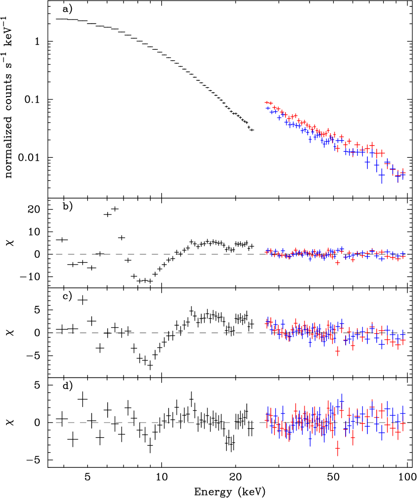
We first discuss joint fits to the long-term PCA/HEXTE spectra, plotted in Figure 2. In these fits, a constant coefficient was included to account for minor normalization offsets between the PCA and HEXTE. The first model tested, a simple power-law modified by cold absorption (Model 1), yielded large residuals near 6 keV due to the presence of the Fe K line; was 2129.17/128 degrees of freedom (). The addition of a Gaussian emission component (Model 2) at 6.38 keV, the Fe K line, was significant at greater than 99.99 confidence in an F-test, as / fell to 586.81/125. However, there still remained broad residuals due to the presence of the Compton reflection component. Model 3 included a pexrav component to model reflection of an underlying power-law component off optically thick and neutral material (Magdziarz & Zdziarski 1995). The inclination angle was assumed to be 30; the power-law cutoff energy was kept fixed at 270 keV as per the results of Perola et al. (1999). Elemental abundances were kept fixed at solar. Adding the pexrav component proved significant at greater than 99.99 confidence in an F-test, since / fell to 208.14/123. The photon index was 1.894. The reflection fraction (defined as /2, where is the solid angle subtended by the reflector) was 0.51 0.04. (With HEXTE data omitted, from PCA data alone is 0.55 0.07; .) Due to the degeneracy between and , it was not possible to fit for both these parameters simultaneously, although we note that for a more face-on inclination (cos() = 0.95), decreased slightly to 0.48 0.04 (with increasing by only 0.1). With the constant coefficient of the PCA fixed at 1.0, the constants for the HEXTE A and B spectra were 0.90 and 0.92, respectively. Table 1 summarizes the model parameters (including line emission parameters) for Model 3. Figure 2 shows the data/model residuals for the three models discussed.
Given the limit of PCA calibration (data/model residuals 2111See http://lheawww.gsfc.nasa.gov/users/keith/rossi2000/energyresponse.ps) and the high signal-to-noise ratio of this spectrum, systematic errors associated with background modeling and the PCA’s spectral response dominated the uncertainties. Finding a statistically acceptable time-averaged fit (with reduced ) was thus unlikely even if the model was representative of the intrinsic spectrum of the source. Additionally, given the low energy resolution of the PCA (1 keV at 6 keV), the PCA is largely insensitive to the detailed shape of the Fe K line; there were no other obvious residuals seen in the Fe K bandpass, e.g., the Fe K emission line was detected only at 90 confidence, and using a diskline model instead of a Gaussian yielded an equally acceptable fit. Model 3 was therefore adopted as a satisfactory baseline fit to the long-term time-averaged PCA/HEXTE spectrum.
Spectral fitting to the medium-term time averaged PCA/HEXTE spectrum proceeded in a manner identical to the long-term spectrum, testing the same three models, and with very similar results, although / was lower due to a lower signal-to-noise ratio. The results of the Model 3 fit are summarized in Table 1. Compared to the long-term time averaged spectrum, the medium-term and were both slightly lower. However, we note the similarity in line emission parameters. Furthermore, the fact that the same type of model was representative of both spectra is consistent with the notion that the general form of the broadband X-ray emission did not change over time.
Since the primary goal of the PCA/HEXTE fitting was to constrain the photon index and the reflection strength , we studed more detailed models only using the higher resolution EPIC-pn data (4). In particular, we adopted = 0.51, the reflection strength from the long-term fits, to use in the EPIC-pn spectral analysis.
4 pn Fits
We now discuss spectral fits to the time-averaged EPIC pn spectrum, shown in Figure 3 (all pn data are plotted with rebinning every 15 bins unless otherwise specified). The best-fitting model was then used as a template for time-resolved spectroscopic studies in 5. We ignored data 2.5 keV and concentrated only on hard X-ray emission. 4.1 describes preliminary fits to the data, including attempts to model the Fe K emission using Gaussians. 4.2 discusses relativistic diskline model fits. 4.3 discusses model fits to a narrow absorption feature seen at 7.68 keV, as well as its detection significance and origin. In 4.4, we present joint pn/RXTE fits. In 4.5, we show that the pn spectrum was consistent with the MOS2 and simultaneous RXTE spectra.
4.1 Fe K and K Emission: Preliminary Fits
Data/model residuals to a simple power-law fit (Model 1) are shown in Figure 3, the Fe K core and Compton reflection hump above 7 keV are clear. Model 2 included a Gaussian near 6.4 keV. For Model 3, a pexrav component with fixed at 0.51 was added. A high-energy cutoff of 270 keV, solar metal abundances, and an inclination of 30 were assumed. Data/model residuals are shown in Figure 4, indicating an excess near 7.0 keV, and a deficit near 7.7 keV suggesting an absorption feature of some kind. The best-fit spectral parameters for Models 1–3 are listed in Table 2. As an alternate parameterization of the Fe K edge, we fit an edge instead of a pexrav component, finding an edge energy of 7.16 0.07 and an optical depth of 0.05 0.01, consistent with Gondoin et al. (2001).
To model the emission near 7.0 keV (the “blue peak”; “red peak” refers to the 6.4 keV line) we added a second Gaussian (Model 4). The best-fit had a blue peak with energy centroid at 6.93 keV and a width of 121 eV. It was significant at 99.99 in an F-test to add this component. Data/model residuals are plotted in Figure 4; the best-fit spectral parameters are listed in Table 2.
In this model, the red peak centroid energy, 6.39 0.01 keV, was consistent with K emission from neutral or mildly ionized Fe. The core width , 91 13 eV, corresponds to a FWHM velocity of 9700 1400 km s-1; this is consistent with the value from Chandra-HETGS, 15100 km (Yaqoob & Padmanabhan 2004). The 6.4 keV line was resolved at the pn resolution of 140 eV: fixing to 1 eV resulted in large data/model residuals while increased by 91. The blue peak was also resolved: fixing to 1 eV caused to increase by 6.5, significant at 99.1 confidence in an F-test.
Given the energy resolution of the pn, it was not obvious from these parameters whether the blue peak was due to neutral Fe K at 7.06 keV, Fe XXVI at 6.966 keV, or a blend of both. To test if it was consistent with being due solely to Fe K, we fixed the blue peak Gaussian’s centroid energy at 7.06 keV and fixed the the KK flux ratio at 0.13. The width was kept tied to . The best fit model (Model 5; see Table 2) was slightly worse than Model 4 ( increased by 7.57), and, as shown in Figure 4, small data/model residuals appeared near 6.8 keV, suggesting excess unmodeled emission on the red side of the blue peak.
The data/model residuals for Models 4 and 5 (see Figure 4) also suggested unmodeled emission on the red side of the K line near 6.1 keV, prompting us to test for the presence of a Compton-scattering shoulder. Such a feature might be expected at 6.24 keV due to Fe K photons Compton-scattering on electrons in the medium in which the line is formed. The shoulder/core intensity ratio indicates scattering in, and an origin for the Fe K line in, Compton-thick or -thin material (ratio above or below 0.1–0.2, respectively; see Matt 2002 for further details). Building on Model 4, we added a third Gaussian emission component with centroid energy fixed at 6.24 keV and a width tied to that for the 6.4 keV core (Model 6). In the best-fit model, the equivalent width was 9 5 eV and the centroid energy was 6.13 keV (it was significant at 98.2 confidence in an F-test to let the centroid energy not be fixed at 6.24 keV). An F-test showed it was significant at 99.6 to add this component (compared to Model 4). Best-fit spectral parameters are listed in Table 3. Considering the pn energy resolution, this feature is consistent with emission from a Compton shoulder. The shoulder-to-core intensity in this case is 0.13, so we cannot rule out either a Compton-thin or Compton-thick origin for the K line. In these models, the Fe K line centroid energies are consistent with emission from neutral or only mildly ionized Fe.
4.2 Fe K and K Emission: Diskline Fits
We now discuss whether relativistic diskline models (Laor 1991) can describe the Fe K profile of IC 4329a. Done et al. (2000) noted from the ASCA observation that IC 4329a seems to have a slightly broadened red wing, though not as broad as that of the “archetypal” broad-line source, MCG–6-30-15 (Tanaka et al. 1995); see Figure 2 of Done et al. (2000). Their best-fit models suggested that there was not significant line emission at radii smaller than 30–100 ( G/). However, compared to the ASCA data, the pn spectrum reveals additional emission and absorption features in the Fe K band; in this section we explore if diskline models can successfully account for all of these features.
As seen by McKernan & Yaqoob (2004), the heights above the power-law continuum of the red and blue peaks in the 60 ksec HEG spectrum were approximately equal, prompting McKernan & Yaqoob (2004) to test if the two peaks could be the horns of a single diskline. Their best-fit model was one with an inclination angle = , rest-frame line energy of 6.74 keV, a flat radial emissivity profile ( 0.7, where the radial emissivity per unit area is quantified as a power law, r-β), and emission between 6 and 70 . However, the current EPIC-pn spectrum clearly shows that the and height above the power-law continuum of the red peak are much greater than those of the blue peak. A relativistic diskline model with near face-on inclination, e.g., 10, can typically produce only one peak, and thus one diskline cannot account for both peaks simultaneously. A diskline model with intermediate or high inclination angles is required to produce clearly-resolved two peaks. We attempted to fit such a model to the pn data, using a Laor diskline (Model 7). We tested inclination angles of 30, 50, and 70. The outer radius was fixed at 400 . In all fits, the inner radius went to very large values, usually 250–350 , with very poor constraints. All fits yielded poor or no constraints on . In all cases, there were large systematic data/model residuals across the Fe K bandpass, as shown in Figure 4 (see also Table 4). The values of for best-fit models were typically 1700–1920 for 1691 , significantly worse fits than e.g., the double-Gaussian model. We conclude that a single-diskline model is an inaccurate description of the data.
The unmodeled excess emission near 6.1 keV and 6.8 keV in the double-Gaussian model (K energy fixed; Model 5) potentially signified that the K and K emission components could each be independently modeled better with a diskline instead of symmetric Gaussian. McKernan & Yaqoob (2004) tested dual-diskline models for the HEG spectrum; the best-fit model was one with a nearly face-on disk, 6, a moderately steep emissivity index = 2.4 0.2, and emission spanning the radii between 6 (fixed) to 600 . S05’s best-fit double-diskline model was found to be consistent with this, with = 1.4, 17, and a profile very similar to a double-Gaussian model. We also fit a double-diskline model to the data, with , , , and for the red and blue disklines set equal to each other, and the normalization of the blue diskline equal to 0.13 that of the red diskline. was kept fixed at 400 ; it was not significant to thaw this parameter. Our best-fit model (Model 8, see Table 5) agrees generally well with that of S05; we found 12, = 2.1 0.3, and 26 . The energy of the red peak was 6.44 keV, more consistent with K emission from mildly ionized Fe than from neutral Fe. The blue peak energy was 6.98 0.09 keV. The equivalent width was 86 eV. The values of and Compton reflection strength were consistent with the prediction of George & Fabian (1991) that, for reflection off neutral material, the reflection strength will be equal to / 150 eV.
For this model, / was 1612.65/1688, similar to that for the Compton shoulder model. As shown in Figure 4, the dual-diskline model accounts well for all of the excess emission-like residuals near 6.1 and 6.8 keV, suggesting that the dual-diskline model is a better description of the data than the double Gaussian models (without a Compton shoulder). To quantify this statement, we replaced only the red peak Gaussian in Model 5 with a Laor component and refitted; / fell to 1621.18/1688, significant at 97.3 confidence in an F-test. Replacing only the blue peak Gaussian with a Laor component and refitting yielded / = 1623.74/1687, significant at only 84.8 confidence in an F-test.
A Laor profile assumes a maximally rotating Kerr black hole. Substituting the Laor model components with diskline model components and assuming a nonrotating Schwarzschild black hole (Fabian et al. 1989) yielded a virtually identical fit to the dual-Laor model For the remainder of this paper, “diskline” will denote the Laor model only.
Finally, we explored the possibility that in addition to the diskline emission, there could be non-negligible emission from narrow components. We added two narrow Gaussians to Model 8 at the rest-frame energies for Fe K and K, with the K normalization set to 0.13 times that of the K line. We first considered the possibility that each broad component is described by a low-inclination diskline component. We kept the widths of both Gaussians fixed at 10 eV. The best-fit model (referred to as Model 9 hereafter) was one with diskline parameters nearly identical to those in Model 8, with the K and K lines contributing only a small amount, and formally consistent with upper limits only in . The best-fit parameters are listed in Table 6. Data/model residuals appeared identical to those in Model 8. A key point here was to determine the maximum allowable for the narrow K line without significantly changing any of the diskline parameters; this was 30 eV, and in this case, the of the broad K line was 51 eV. We conclude that if the dual broad components are described by low-inclination, moderately-relativistic disklines, then the bulk or entirety of the emission must be from the broad components, but a contribution from dual narrow components cannot be ruled out.
We next considered a model wherein high-inclination disklines are responsible primarily for the red-wing emission, with a narrow component accounting for the bulk of the peak emission very close to 6.400 or 7.06 keV. We kept the rest-frame energies of the Fe broad and narrow components fixed at 7.06 keV. Parameters for the best-fit model (henceforth referred to as Model 10) are listed in Table 6. The best-fitting was nearly identical to that for Model 8 (no narrow emission lines). Data/model residuals looked identical to those in Model 8. The width of the narrow K line, 66 eV, corresponds to a FWHM velocity of 7100 km s-1. For Keplerian motion, this corresponds to a radius of 900 (1 2/).
We conclude that if a relativistic diskline is indeed required to best model the emission, then a degeneracy is present: models containing two broad lines and two narrow lines can fit the observed profile of IC 4329a equally well using either a low-inclination diskline (plus little or no narrow emission) or by narrow components plus high-inclination disklines. Alternatively, the Fe K emission profile can be described just as well using Gaussians for the 6.4 and 7.0 keV peaks plus a Compton shoulder with 10 eV. Below, we adopt Model 8, the dual-diskline model with no narrow emission lines, as our ’baseline’ model of the emission profile shape.
To further quantify any possible narrow emission or absorption features in addition to the Fe K and K profiles, we added a narrow Gaussian to Model 8, and, using the steppar command in XSPEC, derived confidence contours of line intensity versus centroid energy. The results are shown in Figure 5, and demonstrate that there were no additional obvious emission or absorption signatures from Fe XXV or XXVI at their rest-frame energies. In fact, the only obvious feature was the narrow absorption feature near 7.7 keV. Fitting narrow Gaussians at the rest-frame energies yielded upper limits in to Fe XXV emission (2 eV), Fe XXV absorption (3 eV), Fe XXVI emission (15 eV), and Fe XXVI absorption (8 eV). The constraints on line emission are stronger than those found by Bianchi et al. (2005) using the 10 ksec XMM-Newton observation of IC 4329a in 2001.
4.3 The 7.68 keV Narrow Absorption Feature
We now focus on modeling the narrow absorption feature at 7.7 keV, which persisted in the data/model residuals independently of how the emission lines were modeled, suggesting a physical origin distinct from that of the emission lines. 4.3.1 discusses simple model fits to the absorption line. In 4.3.2, we show that this feature is likely not an instrumental artifact, and in 4.3.3 we discuss the statistical significance of detecting this feature. 4.3.4 discusses possible origins for the line.
4.3.1 Gaussian Model Fit for the Line
We started with Model 8, the dual-diskline model (though results were independent of which model was used to model the emission profile). We first tested the hypothesis that the feature was indicative of reflection off ionized material, and could be modeled by a K-shell edge due to moderately ionized Fe. Adding an edge (Model 11) yielded a best-fit edge energy of 7.29 keV and an optical depth of 0.03 0.01 (see Table 7). However, the data/model residuals near 7.6 keV were not strongly affected. Forcing the edge energy closer to 7.4–7.6 keV did not improve the data/model residuals. Models incorporating a pexriv component (i.e., in addition to the pexrav component) with 3–10 erg cm s-1 ( 4/; is the 0.5–20 keV ionizing continuum flux; is the density of the reflecting material) similarly proved unsuccessful. We conclude that the feature is too narrow to be an Fe K absorption edge. The lack of an obvious Fe L edge due to moderately ionized Fe also argues against the edge hypothesis.
We then attempted to model the feature using a simple narrow, inverted Gaussian. We returned to Model 8, and added an inverted Gaussian near 7.7 keV (Model 12). The best-fit model successfully removed the data/model residuals, as shown in Figure 4. Spectral parameters for the best-fit Model 12 are listed in Table 7. The best-fit rest-frame energy centroid was 7.68 keV (7.56 keV in the observed frame); was 100 eV. The absolute value of the line intensity was ph cm-2 s-1; was 13 5 eV. The value of / was 1589.46/1685. Compared to Model 8, dropped by 23.19, and an F-test for adding this component yielded a null hypothesis probability of . However, there was no a priori reason to expect an absorption feature at that energy, and so the F-test, when used in this “standard” manner, tends to overestimate the significance of detecting such a feature. The statistical significance of detecting this component will be addressed in more detail in 4.3.3.
4.3.2 PN Background/Instrumental Effects
The pn background spectrum shows no obvious features at 7.56 keV in the observed frame. However, two instrumental features, a Ni K emission line at 7.48 keV and a Cu K emission line at 8.05 keV, are expected (Katayama et al. 2004; Freyberg et al. 2004). These lines originate from the electronics board located below the CCD camera. One might initially suspect that the 7.56 keV (observed-frame) absorption feature could be an artifact resulting from the 7.48 keV line, but there are several arguments against this notion. First, the background count rate is a factor of 40 fainter than that of the source: 5–9 keV count rates in the background and source (after background subtraction) were 0.045 c s-1 and 1.748 c s-1, respectively. As shown in Figure 6, there are no obvious features at these energies in the pn background spectrum of IC 4329a; S05 attempted to detect expected instrumental lines in the pn background to verify the energy scale, but did not detect any with sufficient significance. Second, there were no differences seen in the source spectrum when screened against the periods of highest background rates, as discussed in 2. Third, if it were the case that the 7.48 keV line affects the source spectrum, then one might also expect a feature near 8.05 keV as well, since the 8.05 keV line is actually stronger (Katayama et al. 2004). However, no such features are evident in the source spectrum: adding narrow Gaussians in either emission or absorption at 7.48 or 8.05 keV had no effect on the fit or residuals. Finally, these instrumental lines’ fluxes are at a minimum within 5 of the core (Katayama et al. 2004); the background in this case was extracted over a region located 3 away from the core. We are confident in concluding that the feature at 7.56 keV in the observed frame is intrinsic to the spectrum of IC 4329a and is not an artifact of the instrument or the background.
It has been reported that for pn “double event” data, events where photon energy is deposited on adjacent pixels, the registered photon energy can be 20 eV greater than the energy corresponding to an otherwise-identical single-pixel event (e.g., Pounds & Page 2005). The pn data had initially been extracted using pattern 0–4 events (single and double events); to test for this effect, we re-analyzed the pn data using only single-event (pattern=0) data. For both filtered and unfiltered data, the pattern=0 spectrum was virtually identical to the pattern4 spectrum, though with 30 fewer counts, and a continuum slope that was steeper by 0.05 in photon index. Importantly, however, the fitting results for Fe K bandpass features were virtually identical in all cases. We conclude that the emission and absorption features modeled here are not artifacts of pattern selection.
4.3.3 Estimating the Significance of the Detection of the 7.68 keV Absorption Feature
The standard, two-parameter F-test for the addition of a Gaussian to model the absorption line at 7.68 keV yielded a null hypothesis probability of (4.3 significance). However, using the F-test in this manner has a tendency to overestimate the detection significance, as the F-test does not take into account the possible range of energies where a line might be expected to occur, nor does it take into account the number of bins (resolution elements) present over that energy range. The F-test can yield the probability (equal to one minus the null hypothesis probability) of finding a feature at a given energy if the line energy is known in advance; see e.g., warnings by Protassov et al. (2002). However, in this case, there was no a priori expectation of a 7.68 keV feature, and in searching for narrow features at arbitrary energies, one is searching over many resolution elements and needs to account for the possibility that narrow features can occur by chance due to statistical noise. One might search the 4–9 keV bandpass for Fe K emission/absorption lines, including narrow features near 5–6 keV that have been generally interpreted as gravitationally redshifted Fe K emission (e.g., Turner et al. 2002, 2004). There are about 36 pn resolution elements over this energy range. The probability of detecting a feature at any energy in this range due is found from , where is the number of resolution elements. For IC 4329a, the probability that the 7.68 keV feature is spurious thus becomes (3.4 significance). We note that if the spectral bin sizes are smaller than the instrument resolution, then the number of bins where a line may be located has probably been over-estimated; this means the detection probability may have been underestimated.
Monte Carlo simulations were performed as an additional test of the line significance (see Porquet et al. 2004). These simulations tested the null hypothesis that the spectrum is well-fitted by a model that does not include the 7.68 keV absorption feature. For simplicity, Model 8 (dual disklines) was initially assumed.
We generated 1000 fake spectra as follows: We ran fakeit none on the null hypothesis model, with the photon statistics for a 93.2 ksec exposure, and then re-fit the model to this new fake spectrum, yielding a ”modified” null hypothesis model. We ran fakeit none a second time, using this re-fit model, again with a 93.2 ksec exposure. This was done to account for the uncertainty in the null hypothesis model itself; such uncertainty is relevant, for example, when one is testing for the presence of broad features, when broad features are present in the null hypothesis model, or when the original data set is relatively noisy. This entire process was repeated to generate 1000 fake spectra. For each fake spectrum, we re-grouped to a minimum of 50 counts bin-1 and re-fit the null hypothesis model, obtaining a value (hereafter ). We then added a narrow Gaussian component ( = 10 eV) to the fit. The line normalization was allowed to be positive or negative, to account for the possibility of detecting either an emission or absorption feature, since there had been no a priori expectation for either. We searched over the energy ranges 4.0–6.1 keV and 7.1–10.0 keV. The range 6.1–7.1 keV was excluded to avoid the possibility that the disklines or 7.1 keV pexrav edge would bias the Monte Carlo results. For each fake spectrum, we stepped the Gaussian centroid energy over this range in increments of 0.1 keV (e.g., slightly higher than the instrument resolution), fitting separately each time to ensure that the lowest value of was found. For each fake spectrum, the minimum value of was compared with , yielding a simulated value. Repeating this process 1000 times yielded a cumulative frequency distribution of the expected for a blind line search, assuming the null hypothesis model is correct. We compared this distribution with the observed value, 23.19 in this case. Not a single fake spectrum had 23.19. The inferred probability that the null hypothesis model was correct and that the feature is due to photon noise is thus 0.1; i.e., the 7.68 keV absorption feature is detected at 99.9 confidence.
Similarly, these simulations also can be used to quantify the probability that the Compton shoulder could be due to photon noise. The decrease in when the Compton shoulder was added was 19.1 (comparing models 5 and 6). Monte Carlo simulations, run in the same manner as above, using Model 5 (dual-Gaussian, Fe K energy fixed) as the ’baseline’ model, and searching over 5.8–6.3 keV, yielded no value of observed exceeded in 1000 simulations. The probability that the Compton shoulder is due to photon noise is thus 0.1.
Finally, we briefly address “publication bias”: there are half a dozen XMM-Newton observations of Seyfert 1 galaxies of length and quality (in terms of total number of photons) similar to that of the current observation (e.g., MCG–6-30-15, Fabian et al. 2002; NGC 3783, Reeves et al. 2004). One could thus argue that the significance of detecting the 7.68 keV feature should be reduced to 99.4. We leave it to the reader to include the relevance of such publication bias. However, given the very high value of , the unlikeliness that the feature is an artifact of background modeling, and and the low probability that it could be due to photon noise, we henceforth assume that the 7.68 keV absorption line is intrinsic to IC 4329a and adopt Model 12 as our new baseline model.
4.3.4 The Origin of the Line
As far as the origin of this feature is concerned, there are several candidates to consider. K-shell absorption due to Fe XXV or Fe XXVI is a prime candidate, given that absorption lines attributed to highly ionized Fe have been found in other AGN. If the 7.68 keV line is due to Fe XXVI, then its blueshift suggests an origin in material that is flowing towards the observer with a velocity 31000 km s-1 relative to systemic. If the absorption is due instead to the Fe XXV resonance line (6.697 keV in the rest frame), then the velocity is 44000 km s-1 relative to systemic.
To shed additional light on the origin of this feature, we modified Model 8 (dual-diskline) by including an xstar component (Bautista & Kallman 2001) to model absorption due to ionized material along the line of sight (Model 13). We assumed solar abundances, and kept the redshift as a free parameter. The best-fit model (see Table 7) was one with an ionization parameter characterized by log() = 3.73 erg cm s-1. At this ionization level, Fe K absorption is due almost exclusively to Fe XXVI. The value of /dof was 1584.92/1685, a slightly better fit compared to Model 12. The column density required was cm-2, and the radial velocity shift relative to systemic was –0.093, or –27000 km s-1. The best-fit model is thus consistent with the interpretation above that the absorption feature has an origin in highly ionized material outflowing at 0.1 relative to systemic.
It is not unreasonable to expect supersolar metallicities in AGN environments, given that studies of the BLRs of quasars spanning a range of redshifts generally yield metallicities near or several times solar (e.g., Dietrich et al. 2003a, 2003b). Our fit used solar abundances, but was rather insensitive to the Fe abundance, as one unresolved absorption line cannot break the –abundance degeneracy. For instance, refitting with the Fe abundance fixed at 3 solar yielded cm-2 (no change in ).
It is unlikely that the 7.68 keV feature is due to K absorption by highly ionized Fe (greater than Fe XVII), otherwise one would expect strong K absorption by the same species. For example, the energy of 7.68 keV is close to the absorption energy for Fe K XXIII or XXIV at the systemic velocity, with an ionization parameter log 2.5–3. In that case, however, we would expect an absorption trough due to all the K transitions from Fe XVII–XXIV, between roughly 7.3 and 7.9 keV, and, moreover, a very strong K absorption trough near 6.5–6.6 keV which is not seen in the data. We can similarly rule out redshifted Fe K XXV or XXVI resonant absorption (redshifts of 0.024 and 0.075 relative to systemic, respectively). In these cases, we would expect to see strong Fe K XXV or XXVI resonant absorption at similar redshifts. However, there are no obvious data/model residuals at those energies, and forcing a narrow Gaussian at those energies yields small upper limits on absorption, a few eV for either case.
It is unlikely that the 7.68 keV feature is due to blueshifted K absorption from lowly ionized Fe (7.1–7.2 keV in the rest frame). This would require the absorbing gas to have an ionization parameter smaller than log 2.1. For an absorber with log = 2.0 and a blueshift of 0.068 relative to systemic, a column density of cm-2 is required to fit the 7.68 keV line. However, this model introduces very strong spectral curvature below 4 keV; such curvature is not seen in the EPIC spectrum, as XSTAR modeling using low ionization photo-ionized absorbers yield poor fits to the pn spectrum below 4 keV for column densities above roughly 1021 cm-2 (as shown in Figure 7a). Additionally, for log in the range 1.5–2.1, Fe K absorption is just as strong, or stronger than, Fe K absorption. If the 7.68 keV line were from lowly ionized Fe K, then we would expect Fe K absorption at the same blueshift, near 6.9 keV (source frame). There are no obvious residuals near this energy; forcing an inverted narrow Gaussian into the model yields no change in the fit, with 2.8 eV. One can alleviate the requirement of having Fe K absorption by noting that K absorption is negligible compared to K for log 1.2. In that case, the dominant species will be XVII; the L-shell is full, so K absorption cannot be produced. However, as above, the required column density would introduce very strong spectral curvature into the spectrum below 4 keV, which is not seen. An origin for the 7.68 keV absorption feature in Fe K thus seems unlikely.
We next considered an origin in very highly blueshifted, moderately ionized Fe K (Fe XVII–XXII, rest-frame energies 6.44–6.51 keV). For instance, an xstar absorber with log = 2.1 0.2, a column density cm-2, blueshifted by 0.16 0.01 relative to systemic provided almost as good a fit above 3 keV as Model 13, with / = 1597.41/1685. Absorption due to a range of Fe species creates a trough; for this low a column, the trough is not deep, but at the resolution of the pn, the absorption feature has 12 eV and yielded a similar fit to a narrow Fe XXVI line. However, extrapolation of this model to energies down to 0.9 keV revealed large data/model discrepancies. Specifically, one expects very strong ( = 25–30 eV) absorption features near rest-frame energies of 0.91–0.94 keV due to L-shell absorption by moderately ionized Fe ( XIX–XX) and near 1.86 keV, likely due to Si XIV. For an absorber blueshifted by 0.16, we expect such features to appear at 1.06 and 2.13 keV, but the pn data at those energies show no such features ( 1 eV). More generally, the lack of any strong, highly blueshifted Fe L absorption lines and edges (S05) argues against intermediate species of Fe. An origin in very highly blueshifted Fe XVII thus seems unlikely.
There are transitions around 7.6–7.8 keV associated with highly ionized Ni K (XXV – XXVI or so), but an origin in Ni K with a velocity near systemic is unlikely unless Ni is many times overabundant compared to Fe in IC 4329a.
A local (z=0) origin should be discussed as well, given that several recent soft X-ray AGN spectra have revealed evidence for absorption due to the local hot interstellar medium (e.g., McKernan, Yaqoob & Reynolds 2004). In the case of IC 4329a, a local origin for the line would require an origin in K absorption from intermediate ionized Fe ( XXII). However, an accompanying K line would be expected in this case. Furthermore, the very high column density required to produce such a line (1022 cm-2) is an implausible physical description of the local hot interstellar medium. Similarly, the relativistic velocities required for strongly blueshifted Fe K absorption are not associated with the local hot interstellar medium. We conclude that a local origin for the line is unlikely.
Finally, Figure 7b shows a model spectrum of the effect of the soft X-ray absorbing components seen in S05 on a simple power-law continuum. These low- and moderately ionized components are too low in column density to introduce strong spectral curvature above 4 keV, suggesting that our emission and absorption modeling of the Fe K bandpass is robust.
4.4 Joint PCA/HEXTE/pn Fits
We applied our best-fitting XSTAR model to the pn and long-term RXTE spectra, fitting simultaneously. Constant offsets were included to account for cross-instrument normalizations. When the photon indices for all three instruments were tied, we obtained a best-fit with / = 2140.67/1808 and = 1.827 0.008. Allowing the photon index for the pn to differ resulted a much better fit, as / dropped to 1848/1807. The best-fit model had a Laor inclination of 10 7; we then re-fit with the pexrav inclination fixed at 10 The best-fitting spectral values are listed in Table 8.
4.5 Consistency Checks
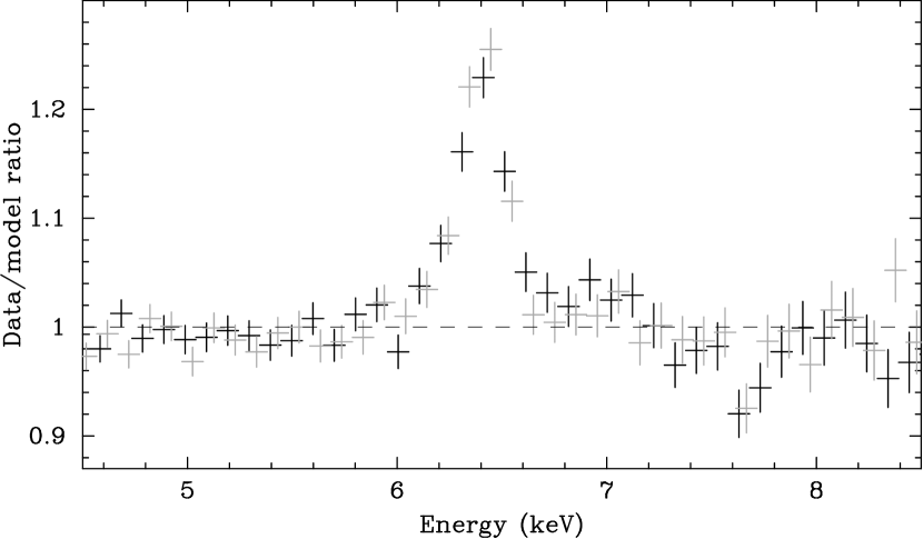
We checked for consistency between the pn and the MOS2 by applying the above models to the MOS2 data between 2.5 and 12 keV. Figure 8 shows the pn and MOS2 residuals to models consisting of a power-law plus pexrav, modified by neutral absorption; the shape of the Fe K profiles are overall similar. Applying the models above to the MOS2 data yielded quite similar fits, with most spectral parameters consistent between the two instruments, though the photon indices for the MOS2 spectra were about 0.15 steeper. We were able to confirm that the Fe K line is detected in the MOS2 data at 90 confidence, using an F-test to compare models 3 and 4. However, due to the lower signal-to-noise ratio in the MOS2, it was not possible to unambiguously verify the existence of the 7.68 keV absorption line ( 29 eV) or confirm that a dual-diskline model was a better fit than a double-Gaussian model.
To check for consistency between the pn and the RXTE PCA, we
generated a “7 day” simultaneous
PCA spectrum using RXTE data taken from the 36 obsids that occurred
within 3.5 days of the midpoint of the XMM-Newton observation.
This resulted in a PCA spectrum with a good exposure time of 19.6 ksec,
enough to
confirm that an Fe K line is present, but not enough to detect
other Fe K bandpass spectral features. The photon index
for Model 3 (Fe K line only), applied to the “7 day” spectrum, was
1.89 0.04, steeper than that of the model when applied to the pn data.
The 2–10 keV flux from the
“7 day,” medium-term and long-term modeled spectra are
erg cm-2 s-1,
erg cm-2 s-1,
and erg cm-2 s-1, respectively.
These values are about 30 higher
than the 2–10 keV flux estimated from model fits to the XMM-Newton pn
spectrum, erg cm-2 s-1.
This discrepancy with the PCA normalization
has been noted previously; see, e.g.,
Yaqoob et al. (2003)222This issue is also discussed in an ASCA Guest Observer Facility
Calibration memo at
http://heasarc.gsfc.nasa.gov/docs/asca/calibration/3c273_results.html.
5 Time-Resolved Spectral Fitting
Studying the time-resolved variability of the Fe K line and continuum components provides a complementary analysis to single-epoch spectral fitting. The simplest models predict that if the reprocessing time scale is negligible, then variations in the Fe K line flux should track continuum variations, modified only by a time delay equal to the light travel time between the X-ray continuum source and the Fe K line origin. However, recent studies of both broad and narrow Fe K lines have not been able to support this picture (e.g., Iwasawa et al. 1996, 1999; Reynolds 2000; Vaughan & Edelson 2001, Markowitz, Edelson & Vaughan 2003). Most of these studies found that Fe K lines tend to vary much less than the continuum, with no evidence for correlated variability, on any time scale. Markowitz, Edelson & Vaughan (2003) additionally showed that Fe K lines, like the continuum, tend to exhibit stronger variability amplitudes towards relatively longer time scales.
Variability of narrow absorption features has also been reported, e.g., Reeves et al. (2004) found evidence for the narrow Fe XXV absorption line in the XMM-Newton spectrum of NGC 3783 to increase in equivalent width over a day, suggesting an origin close to the central X-ray illuminating source. We investigated time-resolved spectroscopy IC 4329a to search for changes in the profile, fluxes, or peak energy of the Fe K emission or 7.68 keV absorption features in IC 4329a, and explore if any such variations are linked to continuum flux variations.
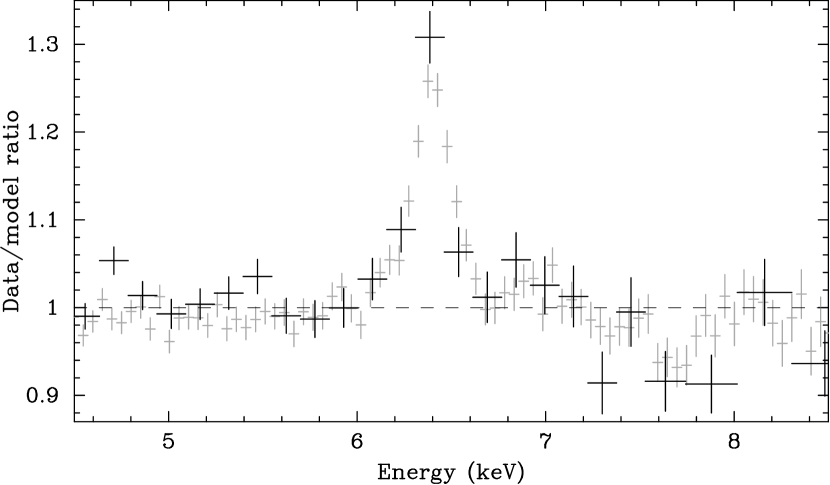
We started with short-term data and split the pn data into two time halves, each covering a duration of 66.3 ksec and with a good time exposure of 46.4 ksec. We fit each spectrum over 2.5–12 keV with Model 12 (dual-diskline plus narrow Gaussian in absorption). The best-fit spectral parameters, listed in Table 9, are all consistent with each other; differences in best-fit values can likely be attributed to less-than-optimal photon statistics. There is no evidence for temporal evolution in any of the absorption and emission profile parameters. The data/model residuals when each spectrum is fitted with a simple absorbed power-law are plotted in Figure 9 and show no obvious changes in the profile. However, given that the hard X-ray continuum light curve (shown in S05) displays minimal variability on these time scales, this is not surprising. Additionally, given the minimal continuum variability, we did not investigate spectral variability as a function of flux, i.e., high/low-flux states.
Next, we performed high time-resolution spectroscopy on all time scales to yield light curves of and the Fe K flux. Time bins were chosen with the goals of achieving adequate signal-to-noise in the Fe K flux light curve. The medium-term data were divided into 18 bins, each covering a duration of 1.972 days, or once every 30 satellite orbits; each bin contained 10 separate RXTE visits. The average exposure time per bin was 5.6 ksec. The long-term data were divided into 18 bins of approximately 44 days each in duration, with no bin overlapping the two 56-day monitoring gaps: data from the periods 2003 Apr 8 to 2003 Sep 29, 2003 Nov 24 to 2004 Sep 30, and 2004 Nov 25 to 2005 Oct 2 were divided into four, seven, and seven bins, respectively. The average good time per bin was 8.1 ksec, excluding bins 3 (100.9 ksec) and 4 (68.7 ksec), which overlapped with the medium-term sampling.
Models were applied to time-resolved data based on the time-averaged fits. The short-term data were divided into eight time bins, with each bin covering a duration of 16.6 ksec and with a good time exposure of 11.6 ksec. Spectral fitting was done over 2.5–12 keV. Model 5 (see Table 2), which featured Gaussians for the Fe K and K emission lines, was used for the short-term spectra. Using the dual-diskline model offered no improvement to the fits; also, the 7.68 keV absorption line was not detected in any RXTE spectrum. For both the long- and medium-term data, Model 3 (see Table 1), which featured a single Gaussian to model the Fe K emission, was used. More detailed fits were not practical, e.g., the Fe K line was not detected. Spectral fitting was done over 3.5–24 keV. The HEXTE statistical errors were too large to study variability, so HEXTE was excluded from the time-resolved analysis. The Fe K line detected in nearly every time bin at 99.8 confidence or greater in an F-test. When fitting the time-averaged models, it was not practical to thaw parameters such as the Fe K line profile shape or peak energy, given the PCA resolution and sensitivity. The neutral absorbing column density was kept as a free parameter. The F-test was used to determine which free parameters to include in the fits. The time-resolved spectral fits were repeated with each of photon index , reflection fraction , and Fe K line normalization frozen at their time-averaged values, and the values of total were compared via an F-test to determine which parameters could justifiably allowed to be free in the fits. The results are shown in Table 10. We found no formal requirement to thaw on any time scale: the total values of decreased only by 0.06 or 0.01 (long and medium, respectively) when was thawed from the time-averaged value. Moreover, when much larger time bins were used to adequately constrain , we found to correlate strongly with , but as noted by Vaughan & Edelson (2001), it is not possible to use the PCA to simultaneously constrain both and in an unbiased fashion, and false correlations can arise. All analysis hereafter assumes is kept fixed at the time-averaged value for each time scale. Strictly speaking, continuum flux should be kept constant in the light of a nonvariable Fe line flux (see below), since both components are expected to have a common origin, but for the current data this does not make any perceptible difference in the fits. As shown in Table 10, it was significant at 99.99 confidence to thaw only on the medium and long time scales, suggesting statistically significant variations in on these time scales. It was significant at 99 confidence to thaw only on the long time scale. Errors on the Fe K line flux and light curves were determined using the point-to-point variance, as discussed in detail by Vaughan & Edelson (2001) and Markowitz, Edelson & Vaughan (2003). The 2–10 keV flux was measured from each model fit. Errors on within a time bin were derived from the 2–10 keV continuum light curves, using the distribution of points within that time bin.
Mean spectral fit values and errors are listed in Table 11. Figure 10 shows the light curves for , , and for all three time scales We note that the long-term averages to the spectral fit parameters shown in Figure 10 and listed in Table 11 do precisely match the spectral-fit parameters to the long-term time average-spectrum listed in Table 1 (see 4.4 for notes comparing the PCA and pn 2–10 keV relative flux normalizations). This is due to the fact that the long-term time-averaged PCA spectrum has a substantial contribution from the medium-term time-averaged spectrum (the medium-term time-averaged spectrum comprises 36 of the long-term spectrum’s total exposure time). Figure 11 shows correlation diagrams for and plotted against . Table 11 also lists the Pearson correlation coefficients and null hypothesis probabilities. Finally, the fractional variability amplitudes, , as defined in Vaughan et al. (2003), are listed in Table 12 for the light curves.
From Figures 10 and 11 and Tables 11 and 12, one can see that there is not much variability in or on short time scales. However, tends to correlate well with on all three time scales, despite the somewhat narrow range spanned by . However, there is no strong evidence for variability in on any time scale; null hypothesis probabilities for a constant line flux cannot be rejected at greater than 60 confidence on any time scale. The lack of variability of the Fe line flux on short time scales has already been reported by S05. The results on long time scales are similar to those of Weaver, Gelbord & Yaqoob (2001), whose did not find any evidence for strong Fe line flux variability in IC 4329a based on five separate ASCA observations between 1993 and 1997.
6 Discussion
The XMM-Newton pn spectrum of IC 4329a reveals an Fe K emission profile with two peaks, identified as Fe K at 6.4 keV and Fe K at 7.0 keV. Modeling the 6.4 keV peak with a simple Gaussian reveals excess emission on the red side of the peak. The red wing can be fit either by a Compton shoulder of 10 eV, or by using relativistic diskline models. 6.1 discusses the emission profile in the framework of relativistic diskline models. The pn spectrum also reveals strong evidence for a narrow absorption feature at 7.68 keV, likely due to H-like Fe K blueshifted by 0.1 relative to systemic, suggesting a highly ionized outflow of some sort. 6.2 discusses the nature of this outflow.
6.1 The Fe K Emission Profile: Moderately Relativistic Disklines
The 6.4 keV peak is much stronger in terms of both and height above the power-law continuum than the 7.0 keV peak, ruling out models wherein both peaks are the Doppler horns of a single relativistic diskline model (e.g., McKernan & Yaqoob 2004). The red peak in particular is not symmetric: a moderate red wing is present, and models incorporating two symmetric peaks do not provide as good a fit to the data as models incorporating at least moderately-relativistic diskline emission from Fe K and Fe K. Alternatively, a dual-Gaussian fit plus a Compton shoulder provides an equally acceptable fit. However, if the redward asymmetry is indeed due to a diskline and not a Compton shoulder, than IC 4329a’s Fe K emission profile is thus distinct from more symmetric and more narrow profiles which lack a red wing, such as that seen in NGC 5548 (Yaqoob et al. 2001, Pounds et al. 2003a). Such narrow, symmetric profiles are generally suspected of having an origin in matter far from the black hole, such as in the outer accretion disk, broad line region, or the molecular torus. In IC 4329a, however, the presence of a moderate red wing leads us to conclude that the emission profile is instead modeled equally well with the following two diskline scenarios: (1) each peak is modeled by a low-inclination, moderately broadened diskline, plus little or no contribution from a narrow emission line, or (2) each peak is modeled as the sum of a narrow line, to account for the emission closest to the rest energy of the line, plus a high-inclination diskline. In the latter case, neither the narrow nor broad component dominates the emission.
In some Seyfert galaxies, identification of broad Fe lines is complicated by model degeneracies which arise when 3–6 keV spectral curvature due to warm absorption is taken into account (e.g., Reeves et al. 2004, Turner et al. 2005). In IC 4329a, however, only minimal spectral curvature above 3 keV, and no spectral curvature above 5 keV, is expected given the results of soft X-ray absorption modeling (see Figure 7b), and so the detection of a moderate red wing is robust. The best-fitting model includes emission extending in to a radius of 26 , similar to that found by Done et al. (2000) using ASCA. Done et al. (2000) note that IC 4329a’s profile does not seem as broadened and reddened as that of MCG–6-30-15, where the diskline emission extends down to 2–3 and the emissivity index is relatively steep, favoring emission from the central regions of the disk (Wilms et al. 2001; Young et al. 2005). The red wing emission in IC 4329a extends down only to energies of 5.4 keV (Done et al. 2000) or 5.7 keV (this work). Although our analysis cannot formally rule out an inner emission radius of 2, the Fe K emission profile in IC 4329a thus seems to fall into a category between those consisting of narrow lines and those consisting of very strongly relativistically broadened lines.
The lack of variability in the Fe K emission line is consistent with an origin in distant matter, as suggested, e.g., by S05. However, the line profile suggests a nonnegligible contribution from material origin close to the black hole. If in fact the bulk of the Fe K emission originates in the inner accretion disk, as in case (1), then a likely scenario is as follows: assuming that variations in the line track those in the X-ray continuum, modified only by a light travel time delay, the line will not vary strongly unless the continuum does. However, the continuum in IC 4329a does not display strong variability. Even on time scales of 2 years, the peak-to-trough continuum variations do not exceed 50, which simply may not be sufficient to trigger very strong trends in Fe K flux. Similarly, with time bins chosen to maximize the variability-to-noise in the Fe flux light curves, this analysis may simply not be sufficiently sensitive to track small-amplitude trends (50 variations) in line flux.
If there are approximately equal broad and narrow component contributions to the profile, as in case 2), then, for time scales longer than the light-crossing times between the continuum source and the sites of broad and narrow line production, it could again be the case that the lack of variability in either component is a result of the lack of strong continuum variability. However, the PCA is not sensitive enough to distinguish between the broad and narrow components. Specifically, if the narrow component, which comprises 60 of the total line emission, is constant, then the PCA time-resolved spectroscopy will not be sensitive to small changes in the broad component. In any case, the lack of strongly correlated variations between the continuum and line prevents us from making any firm conclusions about using variability to determine the location of the line-emitting material.
6.2 The 7.68 keV Absorption Feature: The Highly Ionized Outflow in IC 4329a
High-resolution spectroscopy of the Fe K band of several AGN has yielded evidence for highly ionized absorbing gas, e.g., NGC 3783 (Reeves et al. 2004) and MCG–6-30-15 (Young et al. 2005). In addition, there is evidence in PG and BAL quasars and one other high-luminosity Seyfert for Fe K lines and/or edges that suggest absorbing gas that is both highly ionized and outflowing at relativistic velocities. For instance, in PG 1211+143 (Pounds et al. 2003b), PDS 456 (Reeves et al. 2003), the BAL quasars APM 08279+5255 (Chartas et al. 2002; Hasinger, Schartel & Komossa 2002) and PG 1115+080 (Chartas et al. 2003), and the Seyfert galaxy Mkn 509 (Dadina et al. 2005), the ionization parameters were typically log 2.5 – 3.7, the outflow velocities spanned 0.08–0.34, and the absorber column densities were typically 1–5 cm-2.
The highly ionized (log 3.7), high-velocity (0.1 blueshift relative to systemic) absorbing material in IC 4329a has a derived ionization parameter and outflow velocity similar to what is found in these objects, though we note that the derived column density for the IC 4329a’s outflow component is about a factor of 10 lower. Nonetheless, we hereby add IC 4329a to this rather small but growing list, noting that IC 4329a is thus the lowest redshift AGN known to exhibit this type of outflow.
To estimate the distance between the central black hole and the outflowing gas, we can use = /( ), where is the number density. is the 2–200 keV illuminating continuum luminosity. We estimate the maximum possible distance to the material by assuming that the thickness must be less than the distance . The column density = , yielding the upper limit /(). We estimate the 2–200 keV flux from our models to be erg cm-2 s-1 (assuming = 70 km s-1 Mpc-1 and = 0.73), which corresponds to erg s-1. This yields cm, or 1.2 pc.
In the aforementioned PG and BAL quasars, the derived mass outflow rates are usually at least 1 yr-1 and on the order of the accretion inflow rate, suggesting that these outflows account for a substantial portion of the total energy budget of the AGN. Under the assumption that the gas is in equilibrium and that the outflow velocity is a constant, the mass outflow rate Ṁout for the IC 4329a component can be derived via conservation of mass: Ṁout = , where is the outflow velocity, is the proton mass, and is the covering fraction, which we will assume is 4/10 sr. Substituting = /, we find Ṁout gm s-1 = 5 yr-1. We note that the actual outflow rate should be lower if there is an extreme degree of collimation, or higher if the outflowing component is not directed along the line of sight.
We can compare this to the inflow accretion rate Ṁacc using = Ṁacc, where is the accretion efficiency parameter, typically 0.1. Using the XMM-Newton 2–10 keV flux of erg cm-2 s-1, we derive an 2–10 keV luminosity of erg s-1. Using the relation of Padovani & Rafanelli (1988), = 59 at =2 keV, and a photon index of 1.75, the bolometric luminosity is thus estimated to be = 32 = erg s-1. We find Ṁacc 0.3 yr-1. The kinetic power associated with the outflow component, estimated as Ṁout, is 31045 erg s-1, roughly the same as the bolometric luminosity. Similar to the situation in the aforementioned quasars, the outflow rate of this particular absorbing component may therefore represent a substantial fraction of the accretion inflow used to power the bolometric luminosity in IC 4329a. Similar calculations on the low-velocity, soft X-ray absorbing components (S05), using the 1–1000 Rydberg ionizing continuum luminosity estimated to be erg s-1, suggest that they, too, are associated with outflow rates that are of the same magnitude or higher than the inflow accretion rate. Our estimate for Ṁout is a rough figure, but the fact that it is an order of magnitude higher than Ṁacc suggests that if the outflow were sustained for very long periods, matter could not be transported into the black hole and it could not grow. A low covering fraction and/or a non-continuous, intermittent outflow is required to simultaneously have an outflow existing and the black hole being fed over time.
The high velocity of this outflow suggests that it may be associated with the accretion disk at a small radius. An explanation commonly invoked for the high-velocity, high-ionization absorbers in that the flow originates in the innermost part of a radiatively driven accretion disk wind (e.g., Proga, Stone & Kallman 2001; King & Pounds 2003), although one caution is that it is generally difficult to accelerate highly ionized ions using radiation pressure alone. In this scenario, the winds must be launched from very close in to the black hole, yet far enough away from the black hole that the outflow velocity exceeds the local escape velocity. For a Keplerian disk, the radius at which the escape velocity is 0.1 will be equal to (/)2 = 100; a radiatively driven wind could thus be applicable to IC 4329a if (neglecting acceleration) the wind is launched from a larger radius.
More specifically, King & Pounds (2003; see also Reeves et al. 2003) demonstrated that objects accreting near the Eddington rate are likely to exhibit radiatively driven winds with substantial column densities, and the outflow rates of these winds may be comparable to the accretion inflow rate. If the flow becomes optically-thick at small radii (10–100 ), extreme velocities and high column densities are likely to the associated with the flow. This scenario may be applicable to the high-velocity absorber in IC 4329a. However, we do not know a priori if the accretion rate of IC 4329a is indeed near Eddington. Uncertainty regarding IC 4329a’s black hole mass prevents precise knowledge about the accretion rate. The reverberation-mapped estimate for (Peterson et al. 2004) is formally an upper limit only, , implying an accretion rate relative to Eddington of / of 0.5 (best estimate, 1.29). Other methods yield higher black hole mass estimates. For example, using the photoionization method (estimating velocity dispersions based on H line widths) to estimate the distance from the central illuminating source to the broad-line region, Wandel, Peterson & Malkan (1999) estimate a black hole mass of . Along another track, Nikolajuk, Papadakis & Czerny (2004) suggest a prescription to estimate on the basis of short-term X-ray variability amplitude measurement, specifically the normalized excess variance, . They estimate = based on short-term RXTE light curves. We rebinned the short-term, pn 2.5–12 keV light curve with a sampling time of 6.8 ksec, to yield a light curve with enough data points (20) to get an accurate measurement of . We found = 0.00136 0.00010 (errors derived using Vaughan et al. 2003); the Nikolajuk et al. (2004) relation yields a estimate of , similar to the Nikolajuk et al. (2004) estimate333We note that the Nikolajuk et al. (2004) method assumes that the power spectral density function (PSD) contains a ’break’ (change in power-law slope from –2 to –1) at temporal frequencies corresponding to time scales larger than the duration over which one is measuring (see Nikolajuk et al. 2004 for derivation, as well as additional assumptions and caveats). PDS measurement for IC 4329a is still in progress, pending accumulation of long-term monitoring data, (A. Markowitz et al., in prep.), but we will assume that the PSD break for IC 4329a corresponds a time scale longer than 136 ksec (as expected for any Seyfert with a black hole mass larger than ; see Markowitz et al. 2003).. This value of the black hole mass places the estimated accretion rate / at 15 1 . A more accurate black hole mass determination, e.g., via more accurate reverberation mapping, is needed to resolve this issue. We can only conclude that we currently cannot rule out an accretion rate close to the Eddington limit, and so a radiatively-driven disk wind cannot be ruled out.
Another problem with the disk-wind scenario is that the 7.68 keV absorption feature is narrow, and consistent with a single component only. A broad range of velocities seems more physically plausible if we are seeing a continuous stream of gas being accelerated from rest to 0.1 (relative to the systemic velocity). However, there are no such indications in the Fe K bandpass of material at lower velocities. These facts suggest that we could be witnessing a discrete, transient, outflowing blob of material as opposed to a continuous flow.
In this case, the average mass outflow rate will be lower than the estimate given above, depending on the duty cycle of ejection. One constraint to note is that there are no indications from the soft X-rays (e.g., S05) for absorption at a similar relativistic outflow velocity, so the absorbing material would have to be in the form of a single blob consisting of a high-ionization component only, with no lowly- or moderately ionized contribution, for such a scenario to be applicable.
In addition to radiatively driven outflows, another mechanism whereby radio-quiet AGN can have material outflowing at relativistic velocities is described by the so-called aborted-jet model of Ghisellini, Haardt & Matt (2004). In this model, radio-quiet accreting black holes launch jets only intermittently, yielding discrete, fast-moving blobs that travel along the black hole rotation axis, as opposed to a jet that is continuously on. Extraction of black hole rotational energy, in addition to accretion energy, provides the energy source. The jet is launched at a velocity less the escape velocity, so blobs reach a maximum radius from the black hole before falling backwards and colliding with later-produced outflowing blobs. In the case of IC 4329a, we could thus be witnessing a singular, transient blob at a particular point in its outward journey, although its location must be 100 for this scenario to apply.
Finally, we note that this high-velocity hard X-ray absorber is unlikely to be directly physically connected to the soft X-ray absorbers seen by S05. The soft X-ray absorbers are likely too low in outflow velocity, column density, and ionization state to be part of the same outflow phenomenon as the hard X-ray absorber, suggesting physically distinct phenomena. There is no evidence that the soft X-ray absorbing material “feeds” or is “fed by” the hard X-ray absorber, and no obvious acceleration/deceleration mechanism.
7 Conclusions
We have presented a detailed analysis of the XMM-Newton pn long-look spectrum of IC 4329a. The Fe K bandpass is dominated by two peaks, identified as neutral or near-neutral Fe K and K emission. Both peaks are resolved; the K peak is estimated to have a FWHM velocity near 10,000 km s-1. There is excess emission on the red side of the 6.4 keV line, near 6.1 keV, and we find that three models can all describe the overall emission profile approximately equally well: (1) a model in which the Fe K and K lines are described by Gaussians, signifying neutral or near-neutral Fe emission, and the 6.1 keV emission is a Compton shoulder; (2) a model in which low-inclination dual-diskline profiles originating in mildly ionized Fe dominate the peaks, with little or no contribution from a narrow component; or (3) a model in which approximately equal contributions from a high-inclination diskline and a narrow component describe each peak. The resolution of an X-ray calorimeter is needed to deconvolve the narrow and broad components and break the degeneracy between these various cases. However, the 6.4 keV peak is much higher in equivalent width and height above the continuum compared to the 7.0 keV peak, ruling out models whereby both peaks are the Doppler horns of a single relativistic diskline. There is no strong evidence for emission or absorption at the systemic velocity by Fe XXV or Fe XXVI. In addition, we have used RXTE monitoring data to extract a PCA + HEXTE spectrum to derive tight constraints on the strength of the reflection component.
We have performed time-resolved spectral fitting on the XMM-Newton long-look and the RXTE monitoring data to probe the variability of the X-ray continuum, photon index and Fe K line flux on timescales spanning a day to 2 years. The photon index and 2–10 keV flux are well correlated. However, there is no strong evidence for variability in the Fe K line on any time scale probed, likely due to the minimal level of continuum variability displayed.
We find strong evidence for a narrow absorption line at 7.68 keV. We have used the Monte Carlo simulation method outlined in Porquet et al. (2004) to confirm the high level of detection significance and constrain the probability that the feature is due to photon noise to 0.1. The Monte Carlo method, as used here, accounts for uncertainty in the model, a minor improvement compared to Porquet et al. (2004). The most likely origin for the line is Fe XXVI, in highly ionized material blueshifted by 0.1 relative to systemic, and with a column cm-2. This phenomenon is similar to what is seen in other high luminosity AGN, including PG and BAL quasars, making IC 4329a the lowest redshift AGN known to exhibit this phenomenon. The mass outflow rate of this component is estimated to a few yr-1, and the associated kinetic power is estimated to be of the same order as the bolometric luminosity, suggesting that the outflow represents at least a substantial portion of the overall energy budget. The outflow may be associated with a radiatively driven disk wind. However, because of the narrow velocity range seen, it is also possible that the absorbing material is in the form of a discrete blob of emission. It is important to find as many of these absorbing features as possible in AGN spectra in order to correctly gauge their frequency of occurrence.
References
- (1) Arnaud, K. 1996, in Astronomical Data Analysis Software and Systems, Jacoby, G., Barnes, J., eds., ASP Conf. Series Vol. 101, p. 17
- (2) Bautista, M.A. & Kallman, T. 2001, ApJS, 134, 139 York: McGraw-Hill)
- (3) Bianchi, S., Matt, G., Nicastro, F., Porquet, D. & Dubau, J. 2005, MNRAS, 357, 599
- (4) Blustin, A.J., Page, M.J., Fuerst, S.V., Branduardi-Raymont, G. & Ashton, C.E. 2005, A&A, 431, 111
- (5) Chartas, G., Brandt, W.N., Gallagher, S.C. & Garmire, G. 2002, ApJ, 579, 169
- (6) Chartas, G., Brandt, W.N. & Gallagher, S.C. 2003, ApJ, 595, 85
- (7) Dadina, M., Cappi, M., Malaguti, G., Ponti, G. & De Rosa, A., 2005, A&A, 442, 641
- (8) Dickey, J. & Lockman, F. 1990, ARAA, 28, 215
- (9) Dietrich, M., Appenzeller, I., Hamann, F., Heidt, J., Jäger, K., Vestergaard, M.& Wagner, S.J. 2003a, A&A, 398, 891
- (10) Dietrich, M., Hamann, F., Shields, J.C., Constantin, A., Heidt, J., Jäger, K., Vestergaard, M.& Wagner, S.J. 2003b, ApJ, 589, 722
- (11) Done, C., Madejski, G. & ycki, P. 2000, ApJ, 536, 213
- (12) Edelson, R. & Nandra, K. 1999, ApJ, 514, 682
- (13) Fabian, A.C. et al. 1989, MNRAS, 238, 729
- (14) Fabian, A.C. et al. 2002, MNRAS, 335, L1
- (15) Freyberg, M. et al. 2004, SPIE, 5165, 112
- (16) George, I.M. & Fabian, A.C. 1991, MNRAS, 249, 352
- (17) Ghisellini, G., Haardt, F. & Matt, G. 2004, A&A, 413, 535
- (18) Gondoin, P. et al. 2001, A&A, 378, 806
- (19) Haardt, F., Maraschi, L. & Ghisellini, G. 1994, ApJ, 432, L95
- (20) Hasinger, G., Schartel, N. & Komossa, S. 2002, ApJ, 573, L77
- (21) Iwasawa, K. et al. 1996, MNRAS, 282, 1038
- (22) Iwasawa, K. et al. 1999, MNRAS, 306, L19
- (23) Katayama, H., Takahashi, I., Ikebe, Y., Matsushita, K. & Freyberg, M. 2004, A&A, 414, 767
- (24) King, A. & Pounds, K.A. 2003, MNRAS, 345, 657
- (25) Laor, A. 1991, ApJ, 376, 90
- (26) Magdziarz, P. & Zdziarski, A. 1995, MNRAS, 273, 837
- (27) Markowitz, A. et al. 2003, ApJ, 593, 96
- (28) Markowitz, A., Edelson, R. & Vaughan, S. 2003, ApJ, 598, 935
- (29) Matt, G. 2002, MNRAS, 337, 147
- (30) McKernan, B. & Yaqoob, T. 2004, ApJ, 608, 157
- (31) McKernan, B., Yaqoob, T. & Reynolds, C.S. 2004, ApJ, 617, 232
- (32) Nevalainen, J., Oosterbroek, T., Bonamente, M. & Colafrancesco, S. 2004, ApJ, 608, 166
- (33) Nikolajuk, M., Papadakis, I. & Czerny, B. 2004, MNRAS, 350, L26
- (34) O’Brien, P. et al. 2001, in “Workshop on X-ray Spectroscopy of AGN with Chandra and XMM-Newton,” MPE Report 279, p. 77
- (35) Padovani, P. & Rafanelli, P. 1988, A&A, 205, 53
- (36) Perola, G.C., Matt, G. & Cappi, M. 1999, A&A, 351, 937
- (37) Peterson, B.M. et al. 2004, ApJ, 613, 682
- (38) Porquet, D., Reeves, J.N., Uttley, P. & Turner, T.J. 2004, A&A, 427, 101
- (39) Pounds, K.A., Nandra, K., Stewart, G.C., George, I.M. & Fabian, A.C. 1990, Nature, 344, 132
- (40) Pounds, K.A., Reeves, J.N., Page, K.L., Edelson, R., Matt, G. & Perola, G.C. 2003a, MNRAS, 341, 953
- (41) Pounds, K.A., Reeves, J.N., King, A.R., Page, K.L., O’Brien, P.T. & Turner, M.J.L. 2003, MNRAS, 345, 705
- (42) Pounds, K.A. & Page, K.L. 2005, MNRAS, 360, 1123
- (43) Proga, D., Stone, J.M. & Kallman, T. 2001, AdSpR, 28, 459
- (44) Protassov, R., van Dyk, D.A., Connors, A., Kashyap, V.L. & Siemiginowska, A. 2002, ApJ, 571, 545
- (45) Reeves, J.N., O’Brien, P.T. & Ward, M. 2003, ApJ, 593, L65
- (46) Reeves, J.N., Nandra, K., George, I.M., Pounds, K.A., Turner, T.J. & Yaqoob, T. 2004, ApJ, 602, 648
- (47) Revnivtsev, M., Sazonov, S., Jahoda, K. & Gilfanov, M. 2004, A&A, 418, 927
- (48) Reynolds, C.S. 2000, ApJ, 533, 811
- (49) Rothschild, R. et al. 1998, ApJ, 496, 538
- (50) Shapiro, S., Lightman, A. & Eardley, D. 1976, ApJ, 204, 187
- (51) Steenbrugge, K.C., Kaastra, J.S., Sako, M., Branduardi-Raymont, G., Behar, E., Paerels, F.B.S., Blustin, A.J. & Kahn, S. 2005, A&A, 432, 453
- (52) Strüder, L. et al. 2001, A&A, 365, L18
- (53) Sunyaev, R. & Titarchuk, L. 1980, A&A, 86, 121
- (54) Swank, J. 1998, in Nuclear Phys. B (Proc. Suppl.): The Active X-ray Sky: Results From BeppoSAX and Rossi-XTE, Rome, Italy, 1997 October 21-24, eds. L. Scarsi, H. Bradt, P. Giommi, & F. Fiore, Nucl. Phys. B Suppl. Proc. (The Netherlands: Elsevier Science B.V.), 69, 12
- (55) Tanaka, Y. et al. 1995, Nature, 375, 659
- (56) Turner, M.J.L. et al. 2001, A&A, 365, L27
- (57) Turner, T.J., Mushotzky, R., Yaqoob, T., George, I.M., Snowden, S.,Netzer, H., Kraemer, S., Nandra, K. & Chelouche, D. 2002, ApJ, 574, L123
- (58) Turner, T.J., Kraemer, S. & Reeves, J.N. 2004, ApJ, 603, 62
- (59) Turner, T.J., Kraemer, S., George, I.M., Reeves, J.N. & Bottorff, M.C. 2005, ApJ, 618, 155
- (60) Vaughan, S. & Edelson, R., 2001, ApJ, 548, 694
- (61) Vaughan, S., Edelson, R., Warwick, R. & Uttley, P. 2003, MNRAS, 345, 1271
- (62) Wandel, A., Peterson, B.M. & Malkan, M. 1999, ApJ, 526, 579
- (63) Weaver, K., Gelbord, J. & Yaqoob, T. 2001, ApJ, 550, 261
- (64) Willmer, C.N.A. et al. 1991, AJ, 101, 57
- (65) Wilms, J. et al. 2001, MNRAS, 328, L27
- (66) Yaqoob, T., George, I.M., Nandra, K., Turner, T.J., Serlemitsos, P.J., Mushotzky, R. 2001, ApJ, 546, 759
- (67) Yaqoob, T., George, I.M., Kallman, T., Padmanabhan, U., Weaver, K. & Turner, T.J. 2003, ApJ, 596, 85
- (68) Yaqoob, T. & Padmanabhan, U. 2004, ApJ, 604, 63
- (69) Young, A.J. et al. 2005, ApJ, 631, 733
- (70)
| Parameter | Long Term | Medium Term |
|---|---|---|
| 208.14/123 | 82.7/101 | |
| 2–10 keV flux (erg cm-2 s-1) | 1.20 10-10 | 1.12 10-10 |
| 25–100 keV flux (erg cm-2 s-1) | 1.78 10-10 | 1.74 10-10 |
| 1.894 | 1.782 | |
| 0.51 0.04 | 0.35 | |
| (keV) | 6.38 | 6.33 0.03 |
| (eV) | 228 50 | 341 54 |
| (10-5 ph cm-2 s-1) | 18.2 | 25.3 1.9 |
| (eV) | 128 | 197 15 |
| (1020 cm-2) | 90 20 | 40 |
Note. — Model parameters for the best-fitting Model 3 (power-law + pexrav + Gaussian) to the PCA/HEXTE data. Errors are 90 confidence for one interesting parameter. , , , and are the centroid energy, width, intensity and equivalent width for the Fe K Gaussian emission component. Fe K line emission was not considered here. The high-energy cutoff in the pexrav component was fixed at 270 keV (e.g., Perola et al. 1999); the inclination was kept fixed at 30. The 25–100 keV flux is based on average of HEXTE cluster A and B model fluxes.
| Model 1 | Model 2 | Model 3 | Model 4 | Model 5 | ||
|---|---|---|---|---|---|---|
| 2598.24/1694 | 1727.57/1691 | 1641.80/1691 | 1622.47/1688 | 1630.04/1691 | ||
| 1.656 | 1.671 | 1.737 0.012 | 1.743 0.013 | 1.742 0.013 | ||
| (1020 cm-2) | 10 | 7 | 16 | 17 | 17 | |
| Red peak | E (keV) | … | 6.40 0.01 | 6.40 0.01 | 6.39 0.01 | 6.40 0.01 |
| … | 106 14 | 91 15 | 91 13 | 93 | ||
| … | 8.8 0.7 | 7.8 | 8.0 | 8.0 0.6 | ||
| (eV) | … | 86 6 | 75 | 76 | 77 6 | |
| Blue peak | E (keV) | … | … | … | 6.93 | 7.06 (fixed) |
| … | … | … | 121 | (= ) | ||
| … | … | … | 1.3 | (= 0.13 * ) | ||
| (eV) | … | … | … | 15 | (= 0.13 * ) | |
Note. — Best-fit spectral parameters for various models. Models 4 and 5 additionally included a Gaussian to model Fe K emission with centroid energy free and fixed, respectively. Line intensities are in units of 10-5 ph cm-2 s-1. A pexrav component was included in all models except 1 and 2, with reflection strength fixed at 0.51. The 2–10 keV flux for Models 4–5 was erg cm-2 s-1. See text for additional details.
| 1611.72/1686 | ||
| 1.744 0.012 | ||
| (1020 cm-2) | 9 | |
| Red peak | E (keV) | 6.40 0.01 |
| 76 | ||
| (10-5 ph cm-2 s-1) | 7.4 | |
| (eV) | 70 | |
| Blue peak | E (keV) | 7.06 (fixed) |
| (= ) | ||
| (10-5 ph cm-2 s-1) | (= 0.13 * ) | |
| (eV) | (= 0.13 * ) | |
| Compton shoulder | E (keV) | 6.13 |
| (= ) | ||
| (10-5 ph cm-2 s-1) | 1.1 0.5 | |
| (eV) | 9 5 | |
Note. — Best-fit spectral parameters to a model with Gaussians for Fe K, Fe K, and Compton shoulder emission.
| 1705.56/1691 | |
| 1.739 0.013 | |
| (1020 cm-2) | 8 |
| (keV) | 6.40 0.01 |
| (10-5 ph cm-2 s-1) | 8.6 |
| 84 | |
| 6 (unconstrained) | |
| 300 | |
| 30 (fixed) |
Note. — The outer radius was fixed at 400 . Results are presented here for an inclination angle of 30; angles of 50 or 70 yielded significantly worse fits.
| 1612.65/1688 | ||
| 1.741 0.013 | ||
| (1020 cm-2) | 14 | |
| Red peak | (keV) | 6.44 0.01 |
| (10-5 ph cm-2 s-1) | 8.9 | |
| 86 | ||
| Blue peak | (keV) | 6.98 0.09 |
| 2.1 0.3 | ||
| 26 | ||
| 12 | ||
Note. — For each Laor diskline component, the outer radius was kept fixed at 400 . The normalization of the blue peak diskline was fixed at 0.13 times that of the red peak.
| Model 9 | Model 10 | |||
|---|---|---|---|---|
| 1610.21 / 1687 | 1614.06 / 1686 | |||
| 1.741 0.013 | 1.743 0.013 | |||
| (1020 cm-2) | 14 | 14 | ||
| Gaussians | Red peak | (keV) | 6.40 (fixed) | 6.39 0.01 |
| 5.9 | 7.2 | |||
| (eV) | 52 | 66 | ||
| Blue peak | (keV) | 7.06 (fixed) | 7.06 (fixed) | |
| 10 (fixed) | 66 | |||
| Laor Disklines | Red peak | (keV) | 6.42 | 6.30 |
| 6.9 3.0 | 4.0 1.8 | |||
| (eV) | 65 28 | 37 17 | ||
| Blue peak | (keV) | 6.83 | 7.06 (fixed) | |
| 2.5 | 1.8 | |||
| 64 | 81 | |||
| 30 | 45 | |||
Note. — Best-fit spectral parameters for a model in which the red peak (Fe K) and blue peak (Fe K) are each modeled by the sum of a narrow Gaussian and a broad Laor diskline. The widths of the two Gaussians were tied. The intensity of the blue peak Gaussian was fixed at 0.13 that of the red peak Gaussian. The inner radii , emissivity index and inclination of the two diskline components were tied. The outer radii of both disklines were kept fixed at 400 . Line intensities are in units of 10-5 ph cm-2 s-1. The intensity of the blue peak diskline was kept fixed at 0.13 that of the red peak diskline. To get a reasonable fit, the centroid energy of the K Gaussian and the rest energy of the K diskline were both kept fixed at 7.06 keV. A pexrav component with = 0.51 was included in the model.
| Model 11 | Model 12 | Model 13 | ||
|---|---|---|---|---|
| 1605.81/1686 | 1589.46/1685 | 1584.92/1685 | ||
| 1.715 | 1.734 0.012 | 1.728 | ||
| (1020 cm-2) | 12 | 12 | 10 | |
| Red peak | (keV) | 6.44 0.01 | 6.44 0.01 | 6.44 0.01 |
| (10-5 ph cm-2 s-1) | 8.0 0.7 | 8.5 | 8.3 | |
| (eV) | 76 6 | 81 | 79 | |
| Blue peak | (keV) | 6.98 | 6.98 0.09 | 6.98 0.09 |
| 2.1 | 2.1 | 2.1 | ||
| 43 | 32 | 29 | ||
| 10 | 12 | 10 | ||
| Edge | (keV) | 7.29 | … | … |
| optical depth | 0.034 0.013 | … | … | |
| Gaussian | (keV) | … | 7.68 | … |
| … | 100 | … | ||
| (10-5 ph cm-2 s-1) | … | 1.0 0.3 | … | |
| (eV) | … | 13 5 | … | |
| Photoionized Abs. | Col. dens. (1022 cm-2) | … | … | 1.4 |
| log (erg cm s-1) | … | … | 3.73 | |
| z (rel. to systemic) | … | … | –0.093 | |
Note. — Spectral parameters for best-fit models which attempt to model the 7.68 keV absorption feature. The feature is too narrow to be modeled by an edge, as demonstrated by Model 11. However, modeling the feature with an inverted Gaussian (Model 12) or using an xstar model (Model 13) proved successful. See text for additional details.
| 1874.75/1807 | ||
| (RXTE) | 1.822 0.010 | |
| (pn) | 1.716 | |
| 0.36 0.04 | ||
| (1020 cm-2) | 9 | |
| Red peak | (keV) | 6.44 0.01 |
| (10-5 ph cm-2 s-1) | 12.8 1.0 | |
| (PCA; eV) | 149 12 | |
| (pn; eV) | 126 10 | |
| Blue peak | (keV) | 6.91 0.07 |
| 2.3 0.1 | ||
| 7 | ||
| 10 7 | ||
| Photoionized Abs. | Col. dens. (1022 cm-2) | 1.2 |
| log (erg cm s-1) | 3.99 | |
| z (rel. to systemic) | –0.093 | |
Note. — Spectral parameters for PCA, HEXTE and EPIC-pn fits using the XSTAR model. The photon indices for the PCA and HEXTE data were tied; that for the EPIC-pn was left free. The inclination of the pexrav component was set at 10, the best-fit inclination of the Laor components. Errors on log pegged at the hard upper limit of 4.00.
| First half | Second half | ||
|---|---|---|---|
| (erg cm-2 s-1) | 9.0 10-11 | 8.8 10-11 | |
| 1457.46/1492 | 1513.21/1490 | ||
| 1.752 | 1.732 | ||
| (1020 cm-2) | 15 | 14 | |
| Red peak | (keV) | 6.46 0.05 | 6.45 |
| (10-5 ph cm-2 s-1) | 8.2 | 8.8 | |
| (eV) | 78 | 86 | |
| Blue peak | (keV) | 7.04 | 7.01 0.12 |
| 3.3 | 2.1 | ||
| 70 | 35 | ||
| 22 | 12 | ||
| Gaussian | (keV) | 7.68 0.06 | 7.69 0.07 |
| 150 | 200 | ||
| (10-5 ph cm-2 s-1) | 1.2 | 0.8 0.5 | |
| (eV) | 15 | 11 7 | |
| F-test to include | 99.8 | 95.8 | |
Note. — Best-fitting model 12, featuring dual-disklines for the Fe K emission peaks and an inverted Gaussian for the 7.68 keV absorption feature, to the first and second halves of the EPIC-pn data. All spectral parameters are consistent with remaining constant over timescales 136 ksec. The final row shows the level of significance to include the inverted Gaussian according to an F-test used in the “standard” manner (see text for details).
| Time | ||||
|---|---|---|---|---|
| Scale | F | Prob | F | Prob |
| Short | 0.15 | 0.99 | 0.02 | 1.00 |
| Medium | 5.53 | 2.3 10-12 | 1.51 | 7.8 10-2 |
| Long | 3.04 | 2.3 10-5 | 2.28 | 1.9 10-3 |
Note. — Results of F-tests to determine which parameters it was significant to thaw in the time-resolved fits. High values of the F-statistic and low-values of the probability (of observing that value of F from a random set of data) indicate that the fits show improvement to thaw that parameter, suggesting statistically significant variations.
| Time | Mean | Mean | Mean | ||||
|---|---|---|---|---|---|---|---|
| Scale | 10-11 ph cm-2 s-1 | 10-5 ph cm-2 s-1 | Prob | Prob | |||
| Short | 8.91 0.12 | 1.771 0.027 | 8.22 1.03 | 0.809 | 1.5 10-2 | –0.099 | 0.82 |
| Medium | 13.29 0.06 | 1.828 0.033 | 20.47 3.43 | 0.819 | 3.2 10-5 | 0.272 | 0.27 |
| Long | 15.62 0.09 | 1.917 0.067 | 16.60 4.12 | 0.656 | 3.1 10-3 | –0.059 | 0.82 |
Note. — Mean values of , and . See text for details on error calculations. The Pearson correlation coefficients in Columns (4) and (6) are for and , respectively, plotted against , as shown in Figure 11. The corresponding null hypothesis probabilities (of achieving that value of from a random set of data) are listed in Columns (5) and (7). See 4.4 for notes relating PCA and pn flux normalizations.
| Time | Continuum | Line |
|---|---|---|
| Scale | () | () |
| Short | 3.46 0.48 | Undef. |
| Medium | 9.34 0.14 | 3.49 13.99 |
| Long | 12.99 0.17 | 5.54 19.42 |
Note. — Undefined fractional variability measurements indicate a measured variance that is smaller than that expected solely from measurement noise.