Superclusters of galaxies from the 2dF redshift survey.
I. The catalogue
We use the 2dF Galaxy Redshift Survey data to compile catalogues of superclusters for the Northern and Southern regions of the 2dFGRS, altogether 543 superclusters at redshifts . We analyse methods of compiling supercluster catalogues and use results of the Millennium Simulation to investigate possible selection effects and errors. We find that the most effective method is the density field method using smoothing with an Epanechnikov kernel of radius 8 Mpc. We derive positions of the highest luminosity density peaks and find the most luminous cluster in the vicinity of the peak, this cluster is considered as the main cluster and its brightest galaxy the main galaxy of the supercluster. In catalogues we give equatorial coordinates and distances of superclusters as determined by positions of their main clusters. We also calculate the expected total luminosities of the superclusters.
Key Words.:
cosmology: large-scale structure of the Universe – clusters of galaxies; cosmology: large-scale structure of the Universe – Galaxies; clusters: general1 Introduction
It is presently well established that galaxies form various systems from groups and clusters to superclusters. Galaxy systems are not located in space randomly: groups and clusters are mostly aligned to chains (filaments), and the space between groups is populated with galaxies along the chain. The largest non-percolating galaxy systems are superclusters of galaxies which contain clusters and groups of galaxies with their surrounding galaxy filaments.
Superclusters of galaxies have been used for a wide range of studies. Superclusters are produced by large-scale density perturbations which evolve very slowly. Thus the distribution of superclusters contains information on the large-scale initial density field, and their properties can be used as a cosmological probe to discriminate between different cosmological models. The internal structure of superclusters conserves information on the galaxy formation and evolution on medium scales. Properties of galaxies and groups in various supercluster environments can be used to study the evolution of galaxies on small scales. Superclusters are massive density enhancements and thus great gravitational attractors which distort the background radiation, yielding information on the gravitation field through the CMB distortion via the Sunyaev-Zeldovich effect, which can be detected using new satellites, such as PLANCK.
Early studies of superclusters of galaxies were reviewed by Oort (oort83 (1983)) and Bahcall (bahcall88 (1988)). These studies were based on observational data about galaxies, as well as on data about nearby groups and clusters of galaxies. Classical, relatively deep all-sky supercluster catalogues were constructed using the Abell (abell (1958)) and Abell et al. (aco (1989)) cluster catalogues by Zucca et al. (z93 (1993)), Einasto et al. (e1994 (1994), e1997 (1997), e2001 (2001)) and Kalinkov & Kuneva (kk95 (1995)).
The modern era of the study of various systems of galaxies began when new galaxy redshift surveys began to be published. The first of such surveys was the Las Campanas Galaxy Redshift Survey, followed by the 2 degree Field Galaxy Redshift Survey (2dFGRS) and the Sloan Digital Sky Survey (SDSS). These surveys cover large regions of the sky and are rather deep allowing to investigation of the distribution of galaxies and systems of galaxies out to fairly large distances from us. Catalogues of superclusters were compiled on the basis of these new surveys by Einasto et al. (2003a , 2003b , hereafter E03a and E03b), Basilakos (bas03 (2003)), Erdogdu et al. (erd04 (2004)) and Porter & Raychaudhury (pr05 (2005)). These observational studies have been complemented by the analysis of the evolution of superclusters and the supercluster-void network (Shandarin, Sheth, & Sahni shandarin04 (2004), Einasto et al. 2005b , Wray, Bahcall et al. wray06 (2006)).
| Sample | RA | DEC | |||
|---|---|---|---|---|---|
| deg | deg | ||||
| 2dFN | 147.5 223 | -6.3 +2.3 | 78067 | 229 | 12.42 |
| 2dFS | 325 55 | -36.0 -23.5 | 106328 | 314 | 18.71 |
So far the attention of astronomers has been focused either on small compact systems, such as groups and clusters, or on very large systems – rich superclusters of galaxies. Modern redshift surveys make it possible to investigate not only these classical systems of galaxies, but also galaxy systems of intermediate sizes and richness classes of various sizes, from poor galaxy filaments in large cosmic voids to rich superclusters. In the present series of papers we shall discuss the richest of these systems – superclusters of galaxies. We shall use the term ”supercluster” for galaxy systems larger than groups and clusters which have a certain minimal mean overdensity of the smoothed luminosity density field but are still non-percolating. They form intermediate-scale galaxy systems between groups and poor filaments and the whole cosmic web.
The main goal of this paper is to compile a new catalogue of superclusters using the 2dFGRS. To get a representative statistical sample we include in our catalogue superclusters of all richness classes, starting from poor superclusters of the Local Supercluster class, and ending with very rich superclusters of the Shapley Supercluster class. In the compilation of a statistically homogeneous and complete sample of superclusters we make use of the possibility to recover the true expected total luminosity of galaxy systems, using weights to compensate the absence of galaxies from the sample which are too faint to fall within the observational window of the survey. The use of weights has some uncertainties, so we have to investigate errors and possible biases of our procedure to recover the total luminosity of superclusters. To investigate selection effects and biases we shall investigate properties of simulated superclusters based on the catalogue of galaxies of the Millennium Simulation of the evolution of the structure of the Universe by Springel et al. (springel05 (2005)). In an accompanying paper we shall investigate properties of superclusters (Einasto et al. 2006a , hereafter Paper II). A similar study using the SDSS is in preparation.
The paper is composed as follows. In the next Section we shall describe the observational and model data used. In Section 3 we shall discuss superclusters in the cosmic web. In Section 4 we shall discuss selection effects and their influence on supercluster catalogues. This section is based on simulated superclusters using the Millennium Simulation. Sect. 5 describes the catalogue itself. In the last section we give our conclusions. The catalogue of superclusters is available electronically at the web-site http://www.aai.ee/maret/2dfscl.html.
| Sample | |||||
|---|---|---|---|---|---|
| Mpc | |||||
| Mill.A8 | 8964936 | 8 | 5.0 | 1444 | 125 |
| Mill.A6 | 8964936 | 6 | 6.3 | 1802 | 125 |
| Mill.A4 | 8964936 | 4 | 7.6 | 2244 | 125 |
| Mill.A1 | 8964936 | 0.5 | 8.75 | 32802 | 125 |
| Mill.F8 | 2094187 | 8 | 5.0 | 1734 | 125 |
| Mill.V8 | 1336622 | 8 | 5.0 | 1325 | 125 |
2 Data
In this paper we have used the 2dFGRS final release (Colless et al. col01 (2001), col03 (2003)) that contains 245591 galaxies. This survey has allowed the 2dFGRS Team and many others to estimate fundamental cosmological parameters and to study intrinsic properties of galaxies in various cosmological environments (see Lahav (lahav04 (2004) and lahav05 (2005) for recent reviews). The survey consists of two main areas in the Northern and Southern galactic hemispheres within the coordinate limits given in Table 1. The 2dF sample becomes very diluted at large distances, thus we restrict our sample to a redshift limit ; we apply a lower limit to avoid the confusion with unclassified objects and stars. In Table 1 is the number of galaxies, is the number of superclusters found, and is the volume covered by the sample (in units ). These numbers are based upon version B of the catalogue of groups by Tago et al (tago06 (2006), hereafter T06). This version of the group catalogue was found using the Friend-of-Friend (FoF) method with a linking length, which increased slightly with distance, as suggested by the study of the behaviour of groups with distance (for details see T06).
The catalogue of groups and single galaxies of T06 gives for all galaxies equatorial coordinates (for epoch 2000), the magnitudes, the morphological parameter , the observed absolute magnitude (and the respective luminosity in Solar units, ), and the estimated total luminosity, , also in Solar units. All magnitudes are given in the photometric system.
Galaxies were included in the 2dFGRS, if their corrected apparent magnitude lay in the interval from to . Actually the faint limit varies from field to field. In calculation of the weights these deviations have been taken into account, as well as the fraction of observed galaxies among all galaxies up to the fixed magnitude limit, this fraction is typically about 0.9, while in rare cases it might become very small. In such cases, to avoid too high values of respective corrections, we have applied the completeness correction only when the completeness is higher than 0.5, otherwise we assumed a value 1, i.e. no completeness correction was applied.
For comparison we used simulated galaxy samples of the Millennium Simulation by Springel et al. (springel05 (2005)). Data on comparison samples are shown in Table 2 (for details see Sect. 4).
3 Superclusters in the cosmic web
3.1 Definition of superclusters
Superclusters have been defined so far either as “clusters of clusters” using catalogues of clusters of galaxies, following Abell (abell (1958), abell61 (1961)), or as high-density regions in the galaxy distribution, following the pioneering study by de Vaucouleurs (deV53 (1953)) of the Local Supergalaxy. Nearby superclusters have been found mostly on the basis of combined galaxy and cluster data (Jõeveer, Einasto, Tago jet78 (1978), Gregory & Thompson gt78 (1978), Fleenor et al. fleenor05 (2005), Proust et al. 2006a , 2006b , Ragone et al. ragone06 (2006)). Until recently, more distant superclusters have been found almost exclusively on the basis of catalogues of rich clusters of galaxies by Abell (abell (1958)) and Abell et al. (aco (1989)). Only in recent years distant superclusters have been found using new deep redshift surveys of galaxies, such as the Las Campanas Redshift Survey, the 2dF Galaxy Redshift Survey, and the Sloan Digital Sky Survey (E03a, E03b, Basilakos bas03 (2003), Erdogdu et al. erd04 (2004) and Porter & Raychaudhury pr05 (2005)).
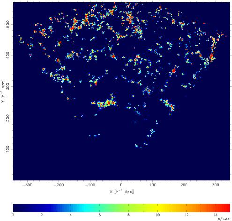
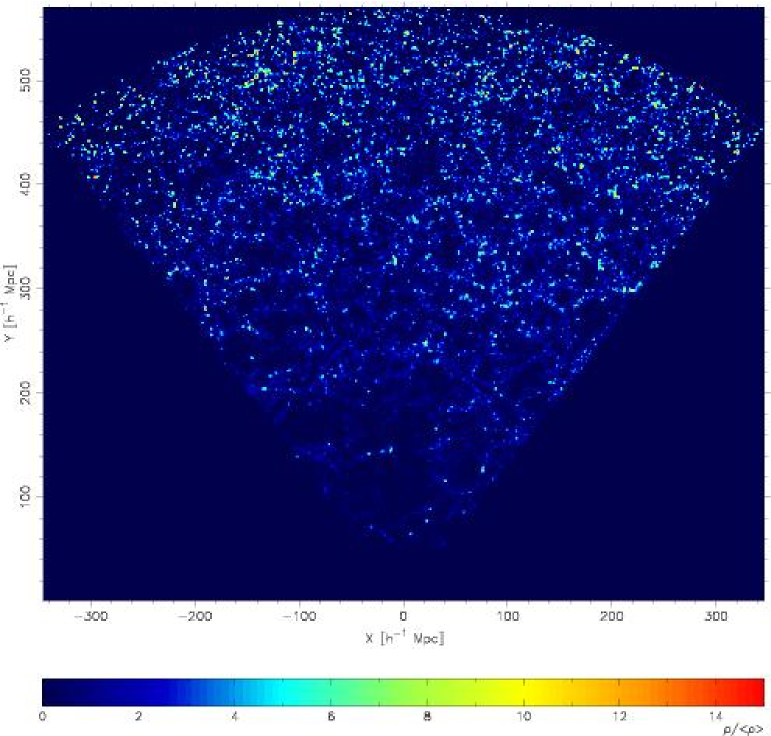
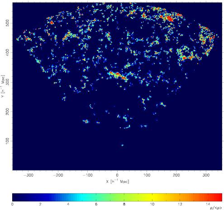
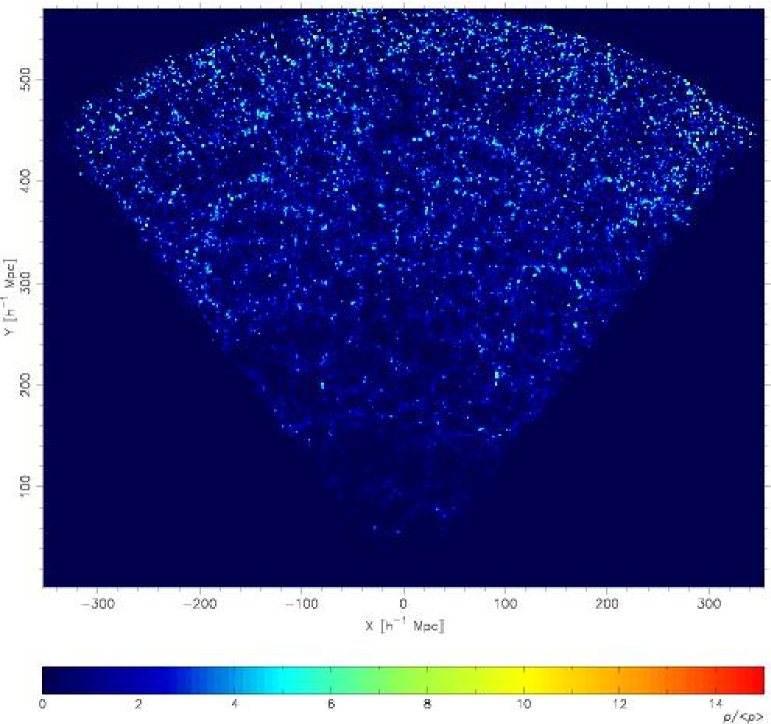
As in previous supercluster searches we are confronted with the problem of how to define superclusters. To visualize the problem we show in Fig. 1 2-dimensional projections of the 2dF Redshift Survey Northern and Southern regions. In these plots luminosity density was found using Gaussian smoothing with rms scale 0.8 Mpc, survey volumes were projected onto a great circle through respective regions of the sky, and the regions were rotated in order have symmetrical areas around the vertical axis. Galaxies and galaxy systems located in different global environments are plotted separately: the left panels show only systems located in high-density environment, and the right panels show only systems in low-density environment. High- and low-density regions are defined by the low-resolution density field smoothed with Epanechnikov kernel of radius 8 Mpc; a threshold density 4.5 was applied in the mean density units.
The comparison of left and right panels shows the presence of a striking contrast between galaxy systems in high- and low-density regions. Luminous systems in high-density regions are fairly compact; they have been conventionally classified as superclusters of galaxies. These systems are well isolated from each other. The majority of these high-density systems are fairly small in size. As we shall see below, these small systems contain only 1 – 2 clusters of galaxies and resemble in structure systems like the Local and the Coma Superclusters. We see also some very rich superclusters: in the Northern region the supercluster SCL126 (Einasto et al. e1997 (1997)) or the Sloan Great Wall (Nichol et al. nic06 (2006) and references therein); and in the Southern region the Sculptor Supercluster SCL9 (Einasto et al. e1997 (1997)).
In contrast, galaxy systems in the low-density region form an almost continuous network of small galaxy filaments. Faint galaxy systems are seen even within large low-density regions (cosmic voids). Most importantly, the distribution of galaxies in space is almost continuous: faint galaxy bridges join groups and clusters, and thus it is a matter of convention, where to put the border between superclusters and poorer galaxy systems.
Traditionally galaxy systems of various scale have been selected from the cosmic web using quantitative methods, such as the Friends-of-Friends (FoF) method or the Density Field (DF) method. In the first case neighbours of galaxies or clusters are searched using a fixed or variable search radius. This method is very common in searching systems of particles in numerical simulations, where all particles have identical masses. The variant with variable search radius has been successfully employed in the compilation of catalogues of groups of galaxies. For the 2dFGRS such catalogues have been published by Eke et al. (2004a ) and Tago et al.(T06). The FoF method was also used by Berlind et al. (berlind06 (2006)) to find groups in the SDSS survey, by Einasto et al. (e1994 (1994), e2001 (2001)) in the compilation of the Abell supercluster catalogues, and by Wray et al. (wray06 (2006)) to find superclusters in numerical simulations. This method is simple and straightforward and especially suitable for volume limited samples, such as the sample of Abell clusters and similar samples of simulated dark matter haloes.
The FoF method has the disadvantage that objects of different luminosity (or mass) are treated identically. Galaxy systems contain galaxies of very different luminosity from dwarf galaxies to luminous giant galaxies. Thus, using the FoF method, it is difficult to make a clear distinction between poor and rich galaxy systems, if their number density of galaxies is similar. The second problem of the FoF method is the complication in using neighbours: the method is simple if a constant linking length (neighbour search radius) is used, but the price for this simplicity is the elimination of faint galaxies from the analysis, in order to get a volume limited galaxy sample.
To overcome these difficulties, the DF method can be used. Here luminosities of galaxies are taken into account, both in the search of galaxy systems, as well as in the determination of their properties. The second advantage of the DF method is the possibility to make allowance for completeness and in this way to restore unbiased values of group (and supercluster) total luminosities.
There exists several variants of the density field method to investigate properties of the distribution of galaxies. Basilakos et al. (bpr01 (2001)) compiled a catalogue of superclusters using the PSCz flux limited galaxy catalogue, using cell sizes equal to the smoothing radius, 5 Mpc and 10 Mpc, for galaxy samples of maximal distance 150 and 240 Mpc, respectively. The use of a fairly large cell size introduces a bias to the density field, which has been corrected. Another variant of the density smoothing is the use of the Wiener Filtering technique, recently applied to the 2dFGRS to identify superclusters and voids by Erdogdu et al. (erd04 (2004)). The data are covered by a grid whose cells grow in size with increasing distance from the observer. Their “target cell width” is set to 10 Mpc at the mean redshift giving a smaller smoothing window for all objects closer and a much larger for galaxies farther away from us.
Our goal is to find superclusters of galaxies, poor and rich, at all distances from the observer until a certain limiting distance. To achieve this goal the selection procedure must be the same for all distances from the observer. For this reason we shall use constant cell size and constant smoothing radius over the whole sample. Of course, random errors of some quantities increase with distance, but we want to suppress systematic bias as much as possible. This allows the identification of smaller systems at all distances from the observer.
The key element in our scheme is the restoration of the expected total luminosity of superclusters as accurately as possible. This goal can be achieved using the weight for galaxies in the calculation of the density field. We have used this approach in estimating total luminosities of superclusters of the Las Campanas Survey and Sloan Early Data Release (E03a, E03b). We shall describe the estimation of expected total luminosities in the next section.
To apply the DF method the luminosity density field is calculated using an appropriate kernel, cell size and smoothing length. An additional parameter which influences the sample, is the threshold density to separate superclusters from poorer galaxy systems. It has the same meaning as the linking length in the FoF method. This is the key parameter which makes a clear distinction between rich and poor galaxy systems, and its influence is illustrated in Fig. 1.
Additionally a certain minimal radius (or volume) of objects must be fixed to avoid the inclusion of noise (too small systems) in our sample. And, finally, certain distance limits must be used for the whole sample to restrict the study to a region covered by observations with a sufficient spatial density of objects. The collection of all these selection parameters defines the final sample of superclusters.
3.2 Calculation of expected total luminosities of galaxies
Due to the selection of galaxies in a fixed apparent magnitude interval the observational window in absolute magnitudes shifts toward higher luminosities when the distance of the galaxies increases. This is the major selection effect in all flux-limited catalogues of galaxies. Due to this selection effect the number of galaxies seen in the visibility window decreases. When calculating estimated total luminosities of galaxies (and groups) we must take this effect into account.
We regard every galaxy as a visible member of a group or cluster within the visible range of absolute magnitudes, and , corresponding to the observational window of apparent magnitudes at the distance of the galaxy. To calculate total luminosities of groups we have to find the estimated total luminosity per one visible galaxy, taking into account galaxies outside of the visibility window. This estimated total luminosity is calculated as follows (E03b)
| (1) |
where is the luminosity of a visible galaxy of an absolute magnitude , and
| (2) |
is the luminosity-density weight (the ratio of the expected total luminosity to the expected luminosity in the visibility window). In the last equation are the luminosity limits of the observational window, corresponding to the absolute magnitude limits of the window , and is the absolute magnitude of the Sun. In the calculation of weights we assumed that galaxy luminosities are distributed according to the Schechter (S76 (1976)) luminosity function:
| (3) |
where and are parameters. Instead of the corresponding absolute magnitude is often used. We take in the band. In calculation of luminosities we used the -corrections according to Norberg et al. (2002MNRAS.336..907N (2002)).
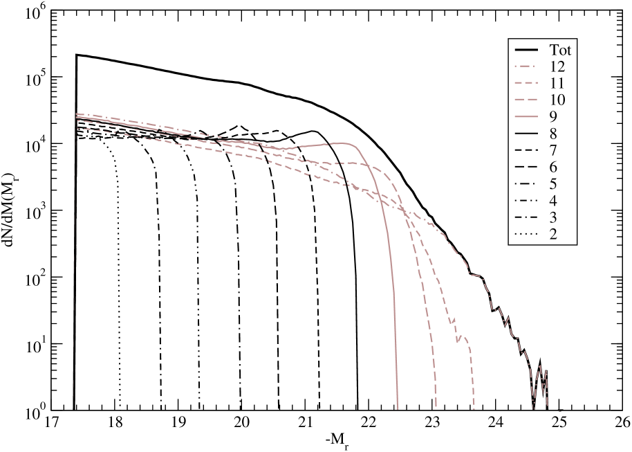
The weights used to calculate estimated total luminosities of superclusters are shown in the Fig. 2. What is important here is not only the absence of faint members of groups at large distance, but also the absence of faint groups. In this paper we are interested in the total luminosities of large systems (superclusters), thus in calculation of estimated total luminosities we use the set of Schechter parameters , , as found by Norberg et al. for the whole 2dF galaxy sample. Our calculations show that this set of Schechter parameters yields total mean luminosity density which is approximately independent of the distance from the observer, as expected for a fair sample of the Universe.
3.3 Preliminary study of 2dFGRS superclusters
We have compiled our 2dFGRS supercluster sample using three steps: 1) a preliminary study of 2dF superclusters to explore the selection parameters and to find the most suitable method to select superclusters; 2) investigation of superclusters in simulated galaxy samples for further analysis of selection parameters and possible biases and errors; 3) selection of the final 2dFGRS supercluster catalogue using parameters chosen during the preliminary study. In the preliminary phase we applied both the FoF and DF methods.
As in the compilation of the group catalogue by T06 we accept the upper limit of redshift of galaxies used in the supercluster search , corresponding to a distance of Mpc. In the calculating distances we use a flat cosmological model with the parameters: matter density , dark energy density (both in units of the critical cosmological density), and the mass variance on 8 Mpc scale in linear theory . Here and elsewhere is the present-day dimensionless Hubble constant in units of 100 km s-1 Mpc-1.
The FoF method is simple when absolute magnitude (volume) limited galaxy samples are used. In this case one can use a constant linking length over the whole sample to find superclusters. We tried two limiting absolute magnitudes, and , with distance limits 400 and 520 Mpc, respectively. A lower limit of the number of galaxies in superclusters of 100 was chosen. Superclusters were selected in the Northern and Southern regions; selection limits in coordinates are given in Table 1.
For the DF method we used a cell size of 1 Mpc. This is the characteristic size of compact galaxy systems – groups and clusters. Using this cell size and a small smoothing length 0.8 Mpc it was possible to follow the distribution of compact galaxy systems (clusters) (E03a, E03b). To characterize the global environment of galaxies a smoothing with characteristic scale 8 – 10 Mpc has been applied, using either a Gaussian or an Epanechnikov kernel, see De Propis et al. (dep03 (2003)), Croton et al. (cr04 (2005)) and Einasto et al. (2005b , hereafter E05b). To avoid excessive smoothing with large wings we used the Gaussian smoothing only to calculate the high-resolution density field with rms scale 0.8 Mpc. To find the low-resolution field we used the Epanechnikov kernel
| (4) |
where is the limiting radius for smoothing. We accepted in the following analysis the radius 8 Mpc.
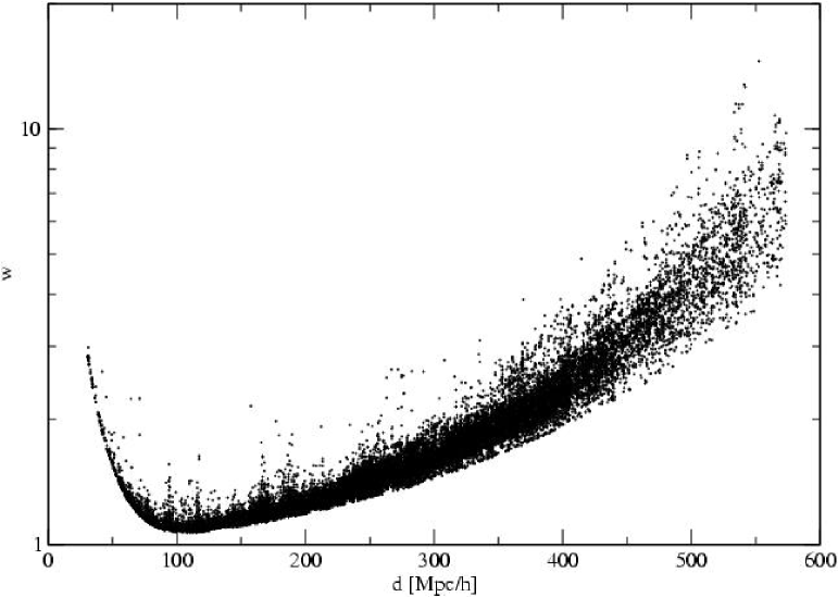
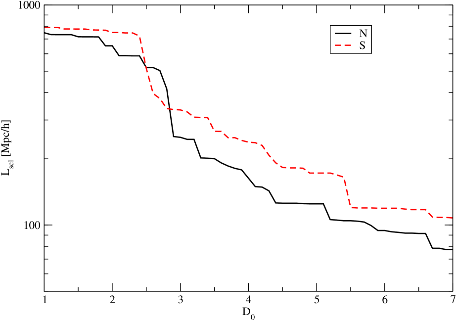
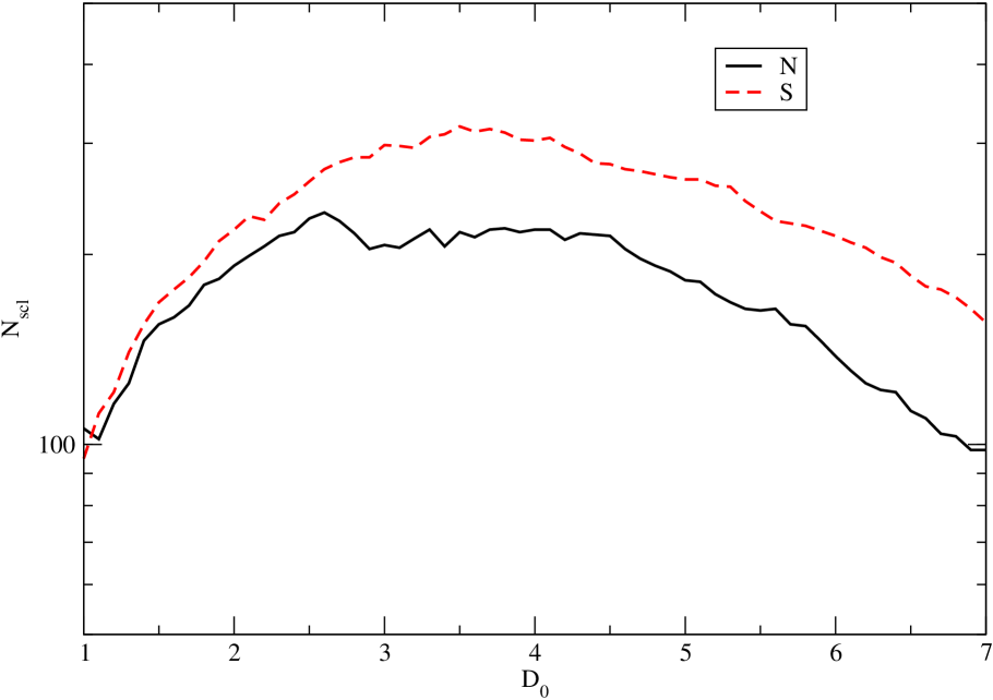
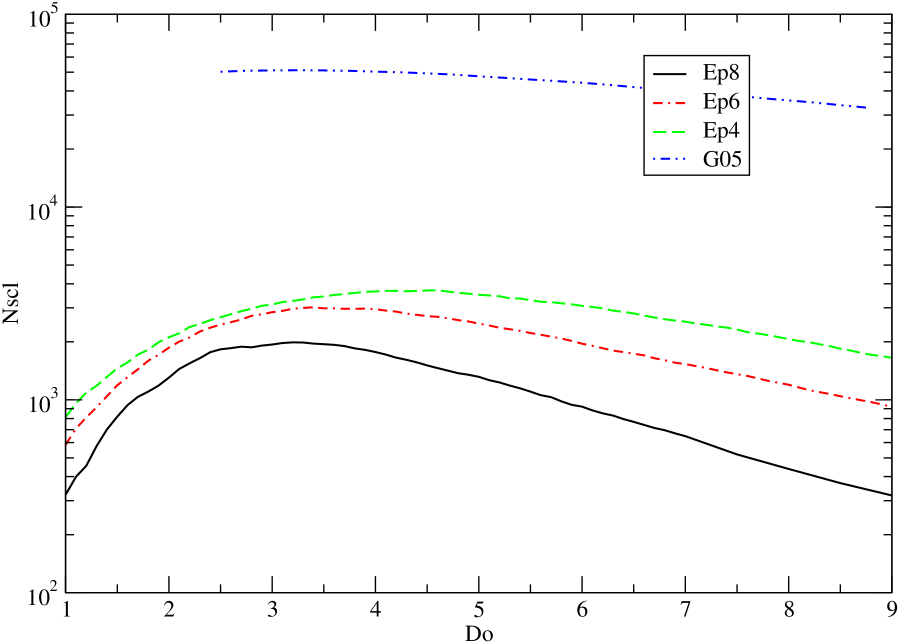
The next step in the selection of superclusters is the proper choice of the threshold density to separate high and low-density galaxy systems. Following E03a we compiled supercluster catalogues in a wide range of threshold densities from 1 to 7 in units of the mean luminosity density of the sample. For each threshold density value we found the number of superclusters, , and calculated the maximal diameter of the largest system found, (see Fig. 3). Detailed supercluster lists and their properties were calculated for several threshold densities in the range 45 (in units of the mean density).
Finally we have to fix the minimal volume (or radius) of systems to be considered as superclusters. This choice is important in order to have a difference between compact galaxy systems, such as groups and clusters, and more extended systems – i.e., superclusters. We take into account the fact that all compact systems transform to extended objects after smoothing. In our previous analysis (E03a and E03b) we used Gaussian smoothing with rms scale 10 Mpc, and the limiting radius of the smallest system to be considered as a supercluster 5.04 Mpc; this radius corresponds to a system of volume 535 ( Mpc)3. When using an Epanechnikov kernel with radius Mpc we can use a smaller limiting radius. Taking these considerations into account we used in our preliminary study 3.63 Mpc as the limiting radius, which corresponds to a limiting volume of 200 ( Mpc)3.
3.4 DF-clusters in superclusters
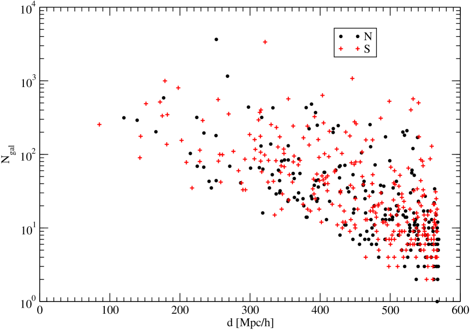
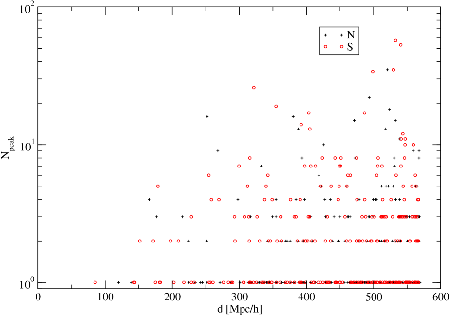
To get an idea of selection effects we show in Fig. 4 the number of galaxies in the superclusters. This number was found by searching for galaxies which lie in the volume above the threshold density level. As we see, the number decreases exponentially with distance. This effect is expected, since galaxies in the 2dFGRS sample are flux-limited, and at larger distances faint galaxies fall outside the observational window. A similar dependence is observed for groups of galaxies of the T06 sample for the same reason: faint distant groups cannot be detected.
This example shows that we cannot use the number of galaxies or groups as the richness criterion of superclusters. Instead of galaxies or groups we can use DF-clusters to characterize the richness of superclusters. The density field is corrected for selection effects using appropriate weights. This approach has been used by E03a and E03b, where lists of DF superclusters and DF-clusters have been compiled. We have followed this experience and have found lists of DF-clusters for all our samples.
To find DF-clusters we used the low-resolution density field, since it averages over the cluster environment, thus giving higher weight to clusters which are located in a high-density environment. In practical terms, all density peaks of the low-resolution density field were located, having a peak density a bit higher than the threshold density used in the supercluster search. We used minimal peak density 5.0 in units of the mean density. The DF-cluster is characterised by its peak density and its integrated peak density found by summing luminosity densities of all cells around the peak together with the central cell in 27 cells. Additionally we searched for galaxies and groups around the central peak within relative distance limits Mpc from the central peak. The smoothed density field integrates luminosities of galaxies inside the whole sphere of radius equal to the smoothing radius, ( Mpc)3, and DF-clusters characterize the luminosity of the central cluster as well as that of surrounding galaxies and groups. This sphere contains in nearby regions 2001000 galaxies and in most distant regions 350 galaxies.
The analysis shows that poor superclusters contain 1 – 2 DF-clusters, i.e. they a similar to the Local and Coma superclusters. In rich superclusters the number of DF-clusters is much higher. The distribution of the multiplicity of superclusters is shown in the right panel of Fig. 4. We see that the distribution is practically independent of the distance. At small distances the number of high-multiplicity superclusters is smaller, but this is a volume effect. What is more important, low-multiplicity superclusters are detected at all distances.
The analysis of properties of superclusters found with the DF and FoF methods demonstrates that the main properties of rich superclusters (positions, diameters, total luminosities etc) are rather stable and do not depend too much on the method to select them. In most cases it was possible to make a one-to-one identification of superclusters found with different methods or sets of selection parameters. Of course, in some cases a rich supercluster found with one method was split into two or more subclusters when a different set of parameters or method was used. As the real cosmic web is continuous, such differences are expected. It is encouraging that these differences were rather small. The only major disadvantage of the FoF method is that a large fraction of the data is not used, since all galaxies fainter than the magnitude limit are ignored. Thus the following analysis was carried out with the DF method only.
4 Analysis of simulated superclusters
The final step in our preliminary study is the analysis of simulated superclusters using the Millennium Simulation. The use of simulated superclusters has the advantage that true properties of model superclusters are known, and the comparison of properties of superclusters based on full data and simulated 2dF data allows us to estimate possible errors and biases of real superclusters.
4.1 Selection effects and biases of the catalogues
The major issue in using flux-limited galaxy samples as the 2dFGRS is the magnitude selection effect. Due to a fixed observational window in apparent magnitudes the range of absolute magnitudes of galaxies (and groups selected from the galaxy sample) changes with the distance. At the far side of the observational sample only very bright galaxies fall into the visibility window of the sample. Thus the number-density of galaxies drops with increasing distance dramatically. This makes it difficult to estimate the true number of galaxies and groups in superclusters.
To investigate selection effects in compiling the catalogue of groups of the 2dFGRS Tago et al (T06) used a simple method: nearby real groups were shifted to larger distance, and the change of the number of group members was investigated. In the present paper we shall use for the study of selection effects simulated galaxies and galaxy systems found in the Millennium Simulation of the structure evolution. For details of the model see Springel et al. (springel05 (2005)), Croton et al. (cr06 (2006)) and Gao et al. (gao05 (2005)). This simulation was made using modern values of cosmological parameters in a box of side-length 500 Mpc, using a very fine grid (about ), and the largest so far number of Dark Matter particles. Using semi-analytic methods simulated galaxies were calculated. The simulated galaxy catalogue contains almost 9 million objects, for which positions and velocities are given, as well as absolute magnitudes in the Sloan Photometric system (u,g,r,i,z). The limiting absolute magnitude of the catalogue is in the r band.
In order to study the influence of the smoothing length we applied an Epanechnikov kernel with radius 4, 6, and 8 Mpc to find the luminosity density field; respective models are marked in Table 2 as Mill.A4, Mill.A6 and Mill.A8 (A for all galaxies used in calculation of the density field). Further we simulated the influence of the observational selection. We put the observer at the lower left corner of the sample at coordinates , calculated distances of every galaxy from the observer, found apparent magnitudes using corrections, and selected galaxies in the observational window of the 2dFGRS , ; this subsample is designated as Mill.F8. To simulate volume-limited galaxy samples we applied a further limit, , in absolute magnitudes in photometric system g (close to system used in the 2dF Survey); this subsample is designated Mill.V8 (in the last samples a smoothing radius 8 Mpc was applied).
One of the first questions to be clarified is: is the luminosity-density relation, observed in the real Universe, also incorporated in simulations? Our experience has shown that it is not always taken into account in simulating galaxies in numerical models. We calculated the density field with a Gaussian kernel of rms scale 0.5 Mpc; this variant is designated Mill.A1. Further we found for every galaxy the local density value at the position of the galaxy, and calculated the number of galaxies in various absolute magnitude intervals separately for different local density environment. In magnitudes we used a step , and for density we used constant intervals in the logarithm of the density with step , starting from density value 0.1 in units of the mean luminosity density.
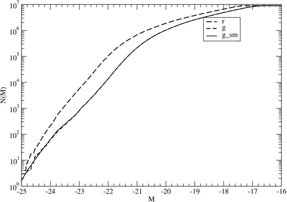
Results of this study are shown in Fig. 5. There are almost no galaxies in the first density bin (). Starting from the second bin each subsequent density bin contains more brighter galaxies, the number of faint galaxies in each bin is approximately constant, and the increase of the maximal luminosity is practically constant, when we move from lower density bins to higher ones. In other words, the luminosity-density relation is built in to the galaxy sample, and we can use the sample to study supercluster properties. The integrated luminosity function for the g and r bands is shown in the right panel of Fig. 5. Due to very large number of galaxies in the sample, the functions are very smooth, and only for the bright end was it necessary to apply a linear interpolation of the function (in representation), also shown in Fig. 5. This luminosity function was used instead of the Schechter law in calculating weights for galaxies according to Eq.2.
4.2 The test for variable smoothing length
We used the density fields calculated with an Epanechnikov kernel with radius 4, 6, and 8 Mpc to select superclusters in a wide range of threshold densities from 1 to 9 in units of the mean luminosity density. For comparison we applied a similar system search also for the high-resolution density field found with a Gaussian kernel and rms scale 0.5 Mpc. In the latter case we used a minimal volume of systems 20 , since this smoothing scale is suitable for the search of compact galaxy systems, such as groups and clusters.
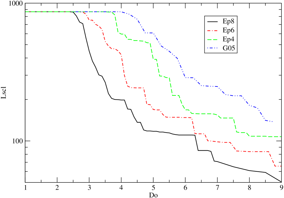
The length (maximal diameter) and the number of systems found are shown in Fig. 6 for all four subsamples. As in the case of real galaxy samples at low threshold density the largest system spans the whole region. To avoid the inclusion of very large percolating systems within our model supercluster catalogue, the threshold density has to be chosen so that the size of the largest system (diameter of the box around the system along coordinate axes) does not exceed a certain value of Mpc. We have chosen values given in Table 2, which correspond to the diameter of the largest supercluster ( Mpc). If one wants to get a higher number of superclusters, then a lower threshold density is to be used, but in this case the size of the largest system exceeds 200 Mpc.
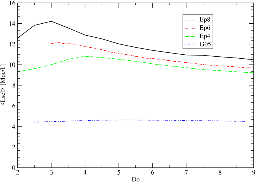
In addition to the diameter of the box around the supercluster we have found also the diameter of the sphere equal to the volume of the superclusters, by counting cells of size 1 Mpc inside the contour surrounded by threshold density level. We call this the effective diameter. Mean values of the effective diameters of superclusters of all samples are shown in Fig. 7 for various threshold density levels. We see that, in spite of the presence of very large percolating superclusters at low threshold density levels, the mean diameters are surprisingly constant. For our accepted threshold levels they lie between Mpc, for superclusters of samples Mill.A4 Mill.A8. The mean diameter of galaxy systems of the sample Mill.A1 is much lower since a lower limiting volume was used in the compilation of this sample.
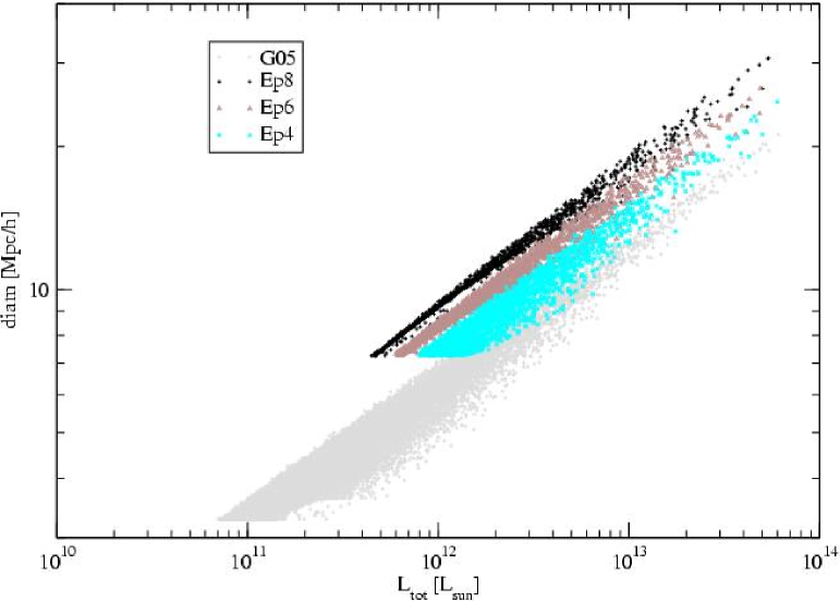
The right panel of Fig. 7 shows the effective diameters of individual superclusters as a function of their total luminosity (found by adding luminosity density values inside the threshold density contour multiplied by the mean luminosity per cell of the whole sample). We see that a very close relationship exists between the diameter and the luminosity of the supercluster. This close relationship is due to the fact that mean densities of superclusters vary in rather narrow limits. The strips of points for various subsamples are shifted with respect to each other: for a given luminosity the supercluster diameter is larger for larger smoothing kernels.
We have cross-correlated individual superclusters of subsamples Mill.A8, Mill.A6 and Mill.A4. For this purpose we find for every supercluster of subsamples Mill.A6 and Mill.A4 the closest supercluster of the sample Mill.A8. In most cases the mutual distance between such supercluster pairs from different subsamples is close to zero, i.e. we have found identical objects in both subsamples. Most very rich superclusters have almost identical counterparts of close total luminosity in different subsamples, as seen in Fig. 8 where total luminosities of cross-identified superclusters are compared. However, the lower the total luminosity of the supercluster the more often a supercluster in subsample Mill.A8 is split into two or more units in subsamples Mill.A6 and Mill.A4. In these cases luminosities of corresponding superclusters of subsamples Mill.A6 and Mill.A4 are lower than in the sample Mill.A8. This explains the presence of numerous dots below the main ridge in Fig. 8.
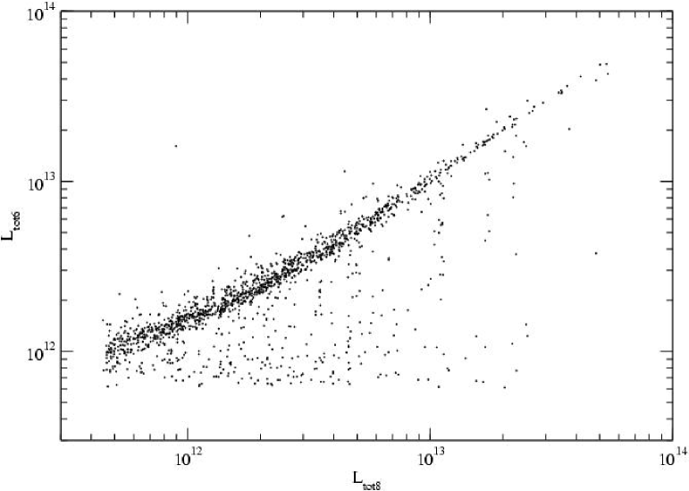
When we compare the distribution of supercluster luminosities of various subsamples, we see that the smaller the smoothing length in calculation of the density field, the higher the number of low-mass superclusters in the subsample. This tendency is seen also in Fig. 8. It is well-known that bridges between high-density knots in the galaxy distribution consist of faint galaxies (due to the density-luminosity relation). If the smoothing length is small then these bridges fall below the density threshold and a galaxy system is considered as consisting of two separate systems. In other words, the density field becomes noisier.
When one uses flux-limited galaxy samples, then at larger distance from the observer fainter galaxies are not visible and bridges between high-density knots cannot be detected. In volume limited samples fainter galaxies are excluded at all distances from the observer. Thus in real galaxy samples faint galaxy bridges disappear at large distance (or everywhere for volume-limited samples). To avoid a too noisy density field it is reasonable to use larger smoothing length. In the following we shall use only supercluster samples found with 8 Mpc smoothing.
4.3 Determination of supercluster centres
It is well-known that rich superclusters are great attractors. This effect is very well seen in numerical models, where it is easy to calculate the potential field. It is natural to identify the centers of superclusters with centres of deepest potential wells inside the supercluster. Rich superclusters have several concentration centres (DF-clusters); the depth of the respective potential wells is different, and only one has the deepest level. In such cases it is relatively easy to identify the dynamical center of the supercluster. The center identification is not so easy in real observational samples. To calculate the potential field the respective density field must be given in a rather large volume. This is easy in numerical models, but difficult in the real Universe, since even the largest modern redshift surveys cover relatively thin slices.
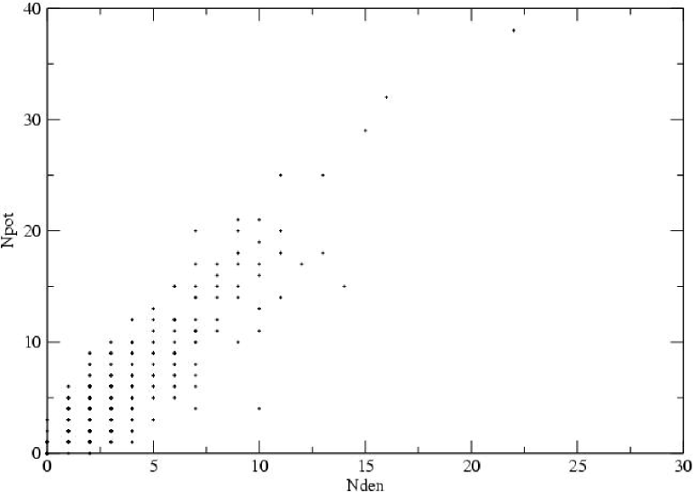
However, it is very easy to identify in real galaxy samples high-density knots of the density field – DF-clusters. The problem is: how well do the positions of high-density knots correlate with positions of depressions in the potential field? To study this problem, we calculated the potential field of the Millennium Survey by Fourier-transforming the high-resolution density field (model Mill.A1). Both fields were calculated on a grid. To have an impression of the fields they were transformed to FITS format and were scrutinized using the ds9 viewer (Smithsonian Astrophysical Observatory Astronomical Data Visualization Application, available for all major operating systems). This viewing impression, as well as the comparison of lists of density peaks and potential field depressions shows that practically all high-density knots in the density field can be recognized as depressions in the potential field.
To obtain a more quantitative relationship between maxima (and minima in case of the potential) of these fields we compared catalogues of maxima of the high-resolution density field and minima of the potential field. Also, in our test catalogues of superclusters extrema of both fields were marked. This comparison shows that the number of peaks of both fields in superclusters is close (see Fig. 9), and that in the majority of cases there exists a one-to-one correspondence between peaks of both fields. In the majority of cases the highest density peak corresponds to the deepest potential well. However, in about 10% superclusters the deepest potential well coincides not with the highest density peak, but with one the following peaks. This occurs mostly in cases where the surrounding potential field has a considerable slope (even within the supercluster), so that absolute values of the depth of the potential well do not always represent the strength of the density peak. Our impression is that in these cases the highest density peak suits even better as the center of the supercluster.
This analysis shows that there are good reasons to consider highest peaks of the smoothed density field as centres of superclusters.
4.4 Analysis of simulated flux-limited samples
We have constructed simulated flux- and volume-limited subsamples of Millennium Simulation galaxies. Using these subsamples we found superclusters and derived their properties for two cases. First, we used the density field of all galaxies, and calculated total luminosities of superclusters for two cases, using full data (Mill.A8 sample) and the simulated 2dF sample Mill.F8. In the second case estimated total luminosities of galaxies were found as for 2dFGRS applying Eq. (2). The luminosity function was taken directly from the simulation data, as shown in Fig. 5. This case allows us to estimate the errors of estimated total luminosities of superclusters using restored galaxy total luminosities. Here the lists of superclusters contain identical entries, only the number of galaxies within them and the estimated total luminosities differ. In this case we do not take into account the fact that the density field also has errors due to the use of incomplete (flux-limited) data.
To get an idea of the scale of the external errors of calculated total luminosities we calculated the smoothed density field using galaxies of the subsample Mill.F8. In this case the identification of superclusters with the first sample is more difficult, since centre coordinates may differ. For identification we identified for every supercluster of the subsample Mill.F8 (and Mill.V8) the closest system among the sample Mill.A8.
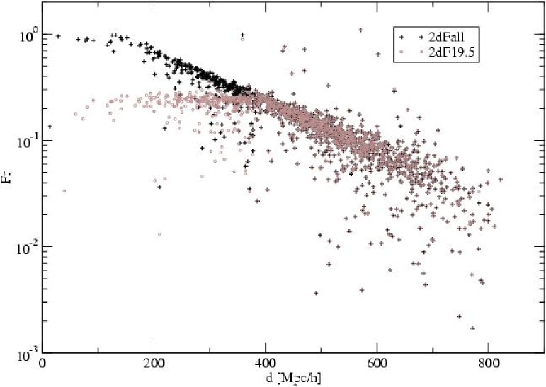
The left panel of Fig. 10 shows the fraction of the number of galaxies in superclusters of subsamples Mill.F8 and Mill.V8 with respect to the respective number in the sample Mill.A8. We see that at small distances this fraction for the subsample Mill.F8 is close to unity, i.e. almost all galaxies are present also in the flux-limited subsample. With increasing distance the fraction gradually decreases. The volume-limited subsample has at large distances from the observer a behaviour similar to the full flux-limited subsample, but on distances less than 400 Mpc the fraction remains constant at a level about 0.2. Some data-points above the main ridge at large distance are due to misidentification of superclusters in our automated procedure.
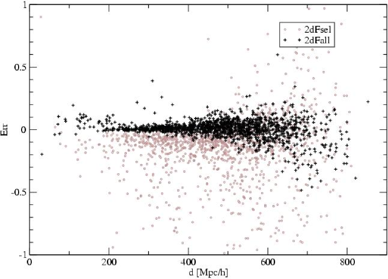
In the right panel of Fig. 10 we plot the relative error of the total luminosity of superclusters as a function of the distance from the observer. Black symbols show internal errors (i.e. supercluster volumes were found using identical density fields, and expected total luminosities were found for complete and simulated 2dF data), gray symbols show external errors (superclusters of the subsample Mill.F8 were found using the density field determined by the same subsample of simulated 2dF galaxies). We see that at large distance from the observer ( Mpc) both internal and external errors become large, since the number of galaxies in superclusters becomes too small. At intermediate distances Mpc internal errors are surprisingly small, and there are practically no systematic errors. External errors are larger, and have a negative tail, i.e. luminosities of superclusters determined from incomplete (flux-limited) data are systematically lower than those calculated using full data. Partly this difference is due to the fact that some superclusters of the sample Mill.A8 are split into smaller systems in the subsample Mill.F8.
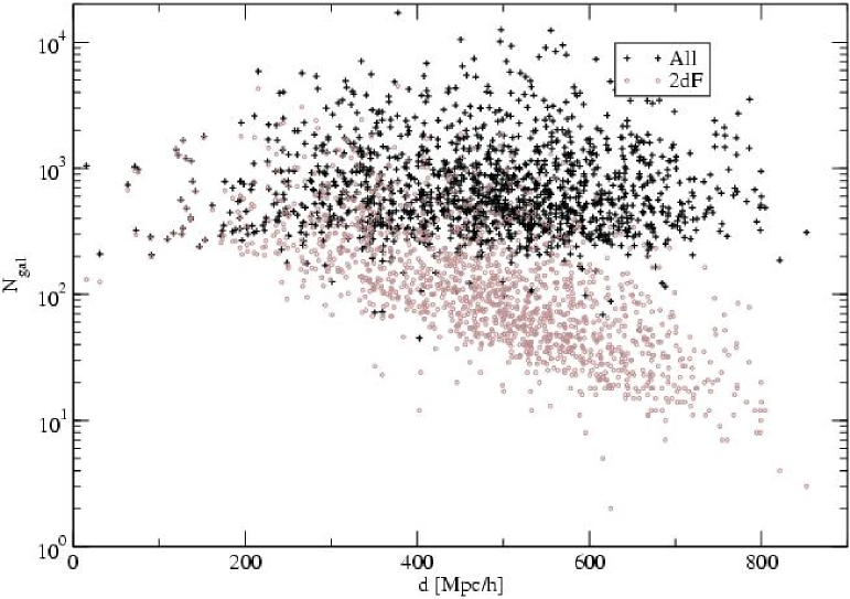
Fig. 11 (left panel) shows the number of galaxies in superclusters of samples Mill.A8 and Mill.F8 as a function of distance. We see that the true number of galaxies in superclusters exceeds 200 with only a few exceptions (remember that the galaxy sample of the Millennium Simulation is complete for luminosities exceeding an absolute magnitude in the r-band). In superclusters identified using flux-limited galaxy samples the number of galaxies decreases with distance. This decrease follows the same law as the fraction shown in Fig. 10 for simulated 2dFGRS superclusters.
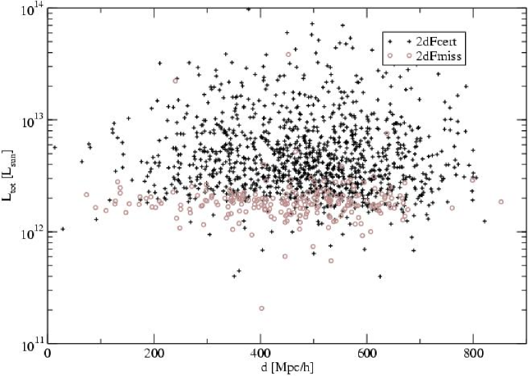
The comparison of lists of superclusters of samples Mill.A8 and Mill.F8 shows that about 200 superclusters of the full sample Mill.A8 have no counterparts in the sample Mill.F8, based on the flux-limited sample of galaxies. In other words, these superclusters are too weak to meet our selection criterion. We show the distribution of luminosities of missing superclusters as a function of distance in the right panel of Fig. 11 by gray symbols. For comparison luminosities of all detected superclusters are also shown. We see that all missing superclusters have low luminosities. In other words, the luminosity function of superclusters found on the basis of flux-limited galaxy samples is biased and needs to be corrected in the range of poor superclusters.
5 2dF supercluster catalogue
Based on the experience of the study of simulated superclusters we shall use for the compilation of the final catalogue of 2dFGRS superclusters the DF method. To calculate the luminosity density field we use an Epanechnikov kernel with radius 8 Mpc, and a rectangular grid of cell size 1 Mpc. To minimize the size of the density field box we treat Northern and Southern regions of 2dF separately. The coordinate system was rotated along the vertical axis so that the sample starts at axis:
| (5) |
| (6) |
| (7) |
where is the minimal value of the Right Ascension for the sample, which is and for the Northern and Southern samples, respectively. After the rotation of coordinates around the -axis both Northern and Southern samples fit in the first quadrant, and coordinates are non-negative. The size of the box along the vertical axis is determined by extreme coordinates of galaxies within the observed regions. Densities were calculated using the total estimated luminosities of galaxies, and then reduced to the mean density over the whole sample. To avoid the inclusion of unobserved regions all cells outside the observational window were marked.
The next step in the selection of superclusters is the proper choice of the threshold density to separate high and low-density galaxy systems. We compiled supercluster catalogues in a wide range of threshold densities from 1 to 7 in units of the mean luminosity density of the sample. For each threshold density value we found the number of superclusters, , and calculated the maximal diameter of the largest system found, . Fig. 3 shows results of these calculations. Based on these data we apply threshold density 4.6 for our final supercluster catalogue. Using this threshold density a few superclusters still have diagonal sizes exceeding 120 Mpc; these superclusters split into subsystems when a larger threshold density is used.
In our preliminary analysis we used a minimal volume 200 ( Mpc)3. The analysis shows that this limit is too high and excludes a number of small superclusters of the Local Supercluster class. Thus in our final catalogue we have used a smaller limiting volume of 100 ( Mpc)3, which corresponds to limiting radius 2.8 Mpc. Using this limit we include practically all galaxy systems which exceed the chosen threshold limit into our supercluster list, and exclude only systems which have a very small fraction of their volume above the threshold. At this level noise due to random errors of corrected galaxy luminosities becomes large. Remember that the use of smoothing with 8 Mpc radius means that all galaxies and groups within this radius are used in the calculation of the density field; thus even the smallest superclusters represent galaxy samples located in a much larger volume than the volume above the density threshold.
The lists of all 2dF groups and single galaxies were searched to find members of superclusters. The number of galaxies in superclusters as a function of the distance from the observer is shown in Fig. 4. As expected, this number decreases with distance. In very poor and distant superclusters the number of galaxies detected may fall below 3. These very poor superclusters have been excluded from our supercluster list. Also, as our analysis of simulated superclusters has shown, some parameters of very distant superclusters have rather large statistical uncertainties. For this reason we have divided our supercluster lists into two parts: the main sample (denoted A) contains superclusters up to distance 520 Mpc, and the supplementary sample (denoted B) has more distant superclusters.
We note that only about 1/3 of all galaxies of the 2dF survey are members of superclusters. The remaining galaxies and groups also belong to galaxy systems, but these systems are weaker and form in the density field enhancements with peak density less than our adopted threshold value 4.6.
We also compiled lists of compact high-density peaks of the density field – DF-clusters, using the low-resolution density field and threshold density 5.0 (in units of the mean density). DF-clusters are some equivalent to rich Abell-type clusters. Since luminosities were corrected to take into account galaxies outside the visibility window, DF-clusters form a volume-limited sample. DF-clusters are useful in the further identification of rich clusters of galaxies of the Abell cluster class. The right panel of Fig.4 shows the distance dependence of the number of DF-clusters in superclusters.
We calculated the luminous mass around the center of DF-cluster in a box containing the parent cell and all surrounding cells (altogether 27 cells). The most luminous group (from the list by T06) in this box was considered as the main group/cluster of the supercluster, and the brightest galaxy of the main cluster was taken as the main galaxy of the supercluster. The center of the supercluster was identified with the center of the main galaxy. Some poor superclusters do not contain peaks above the threshold 5.0 used in the search of DF-clusters. In these cases the most luminous group was considered as the center of the supercluster.
To have an idea of the spatial distribution of luminous matter we can have a look at respective density fields den-Ngr-570-86-ep8.fits and den-Sgr-516-312-ep8.fits on our web-page. These fields can be seen in coordinates using the viewer ds9. We see the multi-nucleus character of most superclusters. Note also the asymmetry of the distribution of galaxies in superclusters.
The final catalogue of 2dFGRS superclusters consists of four lists, two for each Galaxy hemisphere, the main lists A for superclusters up to distance 520 Mpc and supplementary lists B for more distant systems. These lists are given in the electronic supplement of the paper. The lists are ordered according to increasing RA, separately for the Northern and Southern hemispheres, but a common id-numeration for lists A and B. The lists have the following entries.
-
1.
Identification number.
-
2.
Equatorial coordinates (for the epoch 2000).
-
3.
The distance .
-
4.
The minimal size of the supercluster , where , , and are sizes of the supercluster along coordinates ; the sizes are determined from extreme coordinates of the density field above threshold density along coordinate axes.
-
5.
The maximal diameter (diagonal of the box containing the supercluster) .
-
6.
The effective diameter (the diameter of the sphere, equal to the volume of the supercluster).
-
7.
The ratio of the mean to effective diameter: , here is the mean diameter. This parameter characterizes the compactness of the system.
-
8.
The center offset parameter, ; here are coordinates of the geometric center of the supercluster, found on the basis of extreme values of coordinates, and are coordinates of the dynamical center (main cluster) of the supercluster. This parameter characterises the asymmetry of the supercluster.
-
9.
The peak density, (in units of the mean density).
-
10.
The mean density, , (in units of the mean density).
-
11.
The number of galaxies in the supercluster, .
-
12.
The number of groups, (including groups with only one visible galaxy) in the supercluster.
-
13.
The multiplicity of the supercluster, (the number of DF-clusters).
-
14.
The identification of the main cluster according to the group catalogue by T06.
-
15.
The number of visible galaxies in the main cluster.
-
16.
The luminosity of the main galaxy, .
-
17.
The total estimated luminosity of the supercluster, , in photometric system , expressed in Solar units. The total luminosity was found by summing all estimated total luminosities of member groups of the supercluster.
The lists of superclusters of the main catalogue, having total estimated luminosities above , are given in Tables LABEL:tab:Nscl and LABEL:tab:Sscl. The full lists of superclusters, both the main and supplementary, are available at the web-site of Tartu Observatory http://www.aai.ee/maret/2dfscl.html. Density fields in fits format are also available for 2dFGRS and Millennium Simulation samples, see readme.txt for details.
6 Conclusions
In this paper we have used the 2dF Galaxy Redshift Survey to compose a new catalogue of superclusters of galaxies. Our main conclusions are the following.
-
•
To analyse selection effects and possible biases, and to find suitable parameters to select superclusters of galaxies, we analysed simulated superclusters found using the Millennium Simulation of the evolution of the Universe.
-
•
We calculated the density field using the 2dF Galaxy Redshift Survey in the Northern and Southern region, applying smoothing with an Epanechnikov kernel of radius 8 Mpc, and using weights for galaxies which take allowance for faint galaxies outside the observational window of apparent magnitudes.
-
•
Using the smoothed density field we identified superclusters of galaxies as galaxy systems which occupy regions in the density field above the threshold density 4.6 in units of the mean density, and having a minimal volume of 100 ( Mpc)3, separately for the Northern and Southern regions of the 2dFGRS.
-
•
We calculated for all superclusters their main parameters: equatorial coordinates, distances, minimal, maximal and effective diameters, the number of galaxies, groups and DF-clusters, luminosities of main clusters and their main galaxies, total luminosities, overdensities and separation between geometrical and mass center.
-
•
The analysis of the properties of superclusters shows that our supercluster samples are free from known biases.
Acknowledgements.
We are pleased to thank the 2dF GRS Team for the publicly available final data release. The Millennium Simulation used in this paper was carried out by the Virgo Supercomputing Consortium at the Computing Centre of the Max-Planck Society in Garching. This research has made use of SAOImage DS9, developed by Smithsonian Astrophysical Observatory. The semi-analytic galaxy catalogue is publicly available at http://www.mpa-garching.mpg.de/galform/agnpaper. The present study was supported by Estonian Science Foundation grants No. 4695, 5347 and 6104 and 6106, and Estonian Ministry for Education and Science support by grant TO 0060058S98. This work has also been supported by the University of Valencia through a visiting professorship for Enn Saar and by the Spanish MCyT project AYA2003-08739-C02-01. J.E. thanks Astrophysikalisches Institut Potsdam (using DFG-grant 436 EST 17/2/05) for hospitality where part of this study was performed.References
- (1) Abell, G.: 1958, ApJS 3, 211
- (2) Abell, G., 1961, AJ, 66, 607
- (3) Abell, G., Corwin, H., Olowin, R.: 1989, ApJS 70, 1
- (4) Bahcall, N.A. 1988, ARA&A, 26, 631
- (5) Basilakos, S., 2003, MNRAS, 344, 602 astro-ph/0302596
- (6) Basilakos, S., Plionis, M., Rowan-Robinson, M., 2001, MNRAS, 323, 47
- (7) Berlind, A.A., Frieman, J., Weinberg, D.H. et al. 2006, ApJ, astro-ph/0601346
- (8) Colless, M.M., Dalton, G.B., Maddox, S.J., et al. : 2001, MNRAS 328, 1039, (astro-ph/0106498)
- (9) Colless, M.M., Peterson, B.A., Jackson, C.A., et al. : 2003, (astro-ph/0306581)
- (10) Croton, D.J., Farrar, G. R., Norberg, P. et al. 2005, MNRAS, 356, 1155 astro-ph/0407537
- (11) Croton, D.J., Springel, V., White, S.D.M. et al. 2006, MNRAS, 365, 11
- (12) De Propris, R., et al. (2dF GRS Team): 2002, MNRAS 329, 87
- (13) De Propris, R., et al. (2dF GRS Team): 2003, MNRAS 342, 725, (astro-ph/0212562)
- (14) de Vaucouleurs, G., 1953, AJ, 58, 30
- (15) Einasto, J., Einasto, M., Hütsi, G., et al. : 2003a, A&A 410, 425 (E03a)
- (16) Einasto, J., Einasto, M., Saar, E., et al. 2006, (Paper II)
- (17) Einasto, J., Hütsi, G., Einasto, M., et al. : 2003b, A&A 405, 425 (E03b)
- (18) Einasto, J., Tago E., Einasto, M., Saar, E.: 2005a, In ”Nearby Large-Scale Structures and the Zone of Avoidance”, eds. A.P. Fairall, P. Woudt, ASP Conf. Series, 329, 27, (astro-ph/0408463)
- (19) Einasto, J., Tago E., Einasto, M., et al. 2005b, A&A, 439, 45 (E05b)
- (20) Einasto, M., Einasto, J., Müller, V., Heinämäki, P., Tucker, D.L.: 2003c, AA 401, 851
- (21) Einasto, M., Einasto, J., Tago, E., Dalton, G. & Andernach, H., 1994, MNRAS, 269, 301 (E94)
- (22) Einasto, M., Einasto, J., Tago, E., Müller, V. & Andernach, H., 2001, AJ, 122, 2222 (E01)
- (23) Einasto, M., Einasto, J., Tago, E., et al. 2006; A&A (in preparation) (E06)
- (24) Einasto, M., Jaaniste, J., Einasto, J., et al. : 2003d, AA 405, 821
- (25) Einasto, M., Tago, E., Jaaniste, J., Einasto, J. & Andernach, H., 1997, A&A Suppl., 123, 119 (E97)
- (26) Eke, V. R., Baugh, C. M., Cole, S., et al. : 2004a, MNRAS 348, 866, (astro-ph/0402567)
- (27) Erdogdu, P., Lahav, O., Zaroubi, S. et al. 2004, MNRAS,352, 939
- (28) Fleenor, M.C., Rose, J.A., Christiansen, W.A. et al. 2005, AJ, 130, 957 [astro-ph/0512169]
- (29) Gao, L., White, S.D.M., Jenkins, A. et al. 2005, MNRAS, 363, 379
- (30) Gregory, S.A. & Thompson, L.A. 1978, ApJ, 222, 784
- (31) Jõeveer, M., Einasto, J. & Tago, E. 1978, MNRAS, 185, 357
- (32) Kalinkov, M. & Kuneva, I. 1995, A&A Suppl., 113, 451
- (33) Lahav, O. 2004, Pub. Astr. Soc. Australia, 21, 404
- (34) Lahav, O. 2005, In ”Nearby Large-Scale Structures and the Zone of Avoidance”, eds. A.P. Fairall, P. Woudt, ASP Conf. Series, 329, 3
- (35) Mobasher, B., Dickinson, M., Ferguson, H.C. et al. 2005, astro-ph/0509768
- (36) Nichol, R.C., Sheth, R.K., Suto, Y., et al., (astro-ph/0602548)
- (37) Norberg, P., et al.: 2002, MNRAS 336, 907, (astro-ph/0111011)
- (38) Oort, J.H. 1983, Ann. Rev. Astr. Astrophys. 21, 373
- (39) Porter, S.C. & Raychaudhury, S. 2005, MNRAS, 364, 1387 [astro-ph/0511050]
- (40) Proust, D., Quintana, H., Carrasco, E.R. et al. 2006a, AA, 447, 133
- (41) Proust, D., Quintana, H., Carrasco, E.R. et al. 2006b, astro-ph/0509903
- (42) Ragone, C.J., Muriel, H., Proust, D. et al. 2006, AA, 445, 819
- (43) Shandarin, S.F., Sheth, J.V. & Sahni, V., 2004, MNRAS, 353, 162
- (44) Schechter, P. 1976, ApJ, 203, 297
- (45) Springel, V., White, S.D.M., Jenkins, A. et al. 2005, Nature, 435, 629; astro-ph/0504097
- (46) Stoughton, C., Lupton, R. H., Bernardi, M. et al. 2002, AJ, 123, 485
- (47) Tago, E., Einasto, J., Saar, E. et al. 2006, AN, 327, 365 (T06)
- (48) Tucker, D.L., Oemler, A.Jr., Hashimoto, Y., et al. : 2000, ApJS 130, 237
- (49) Wray, J.J., Bahcall, N., Bode, P. et al. 2006, astro-ph/060306
- (50) Zucca, E. et al. 1993, ApJ, 407, 470
- (51) Yang, X., Mo, H.J., van den Bosch, F.C., Jing, Y.P.: 2004, MNRAS 357, 608, (astro-ph/0405234)
| Id | RA | DEC | ||||||||||||
|---|---|---|---|---|---|---|---|---|---|---|---|---|---|---|
| deg | deg | Mpc | Mpc | Mpc | Mpc | Mpc | ||||||||
| 5 | 149.58 | -4.64 | 457.6 | 19.0 | 45.2 | 18.6 | 1.4 | 3.3 | 10.9 | 6.6 | 102 | 5 | 0.3553E+11 | 0.5460E+13 |
| 9 | 150.47 | -0.86 | 398.8 | 19.0 | 37.1 | 15.0 | 1.4 | 9.2 | 5.7 | 5.6 | 52 | 3 | 0.6251E+11 | 0.2675E+13 |
| 13 | 152.01 | 0.57 | 288.1 | 31.0 | 89.7 | 27.5 | 1.9 | 25.3 | 12.9 | 6.9 | 1145 | 10 | 0.4872E+11 | 0.1646E+14 |
| 17 | 153.54 | -4.22 | 467.4 | 20.0 | 66.2 | 21.5 | 1.8 | 8.9 | 9.3 | 6.0 | 120 | 8 | 0.4714E+11 | 0.8309E+13 |
| 20 | 155.11 | -2.54 | 184.5 | 17.0 | 40.0 | 15.5 | 1.5 | 8.2 | 7.2 | 5.7 | 556 | 2 | 0.3929E+11 | 0.3188E+13 |
| 27 | 156.91 | 1.86 | 440.4 | 15.0 | 33.5 | 15.4 | 1.3 | 8.2 | 6.4 | 6.2 | 68 | 4 | 0.1652E+11 | 0.3327E+13 |
| 37 | 160.34 | -5.90 | 384.5 | 18.0 | 67.0 | 22.2 | 1.7 | 28.2 | 12.0 | 6.7 | 359 | 9 | 0.3478E+11 | 0.9555E+13 |
| 38 | 160.57 | -3.74 | 509.6 | 23.0 | 41.6 | 14.6 | 1.6 | 6.8 | 10.5 | 6.3 | 34 | 4 | 0.3574E+11 | 0.3080E+13 |
| 76 | 170.64 | 0.45 | 302.5 | 17.0 | 42.7 | 19.3 | 1.3 | 8.2 | 6.7 | 6.7 | 420 | 5 | 0.4723E+11 | 0.5933E+13 |
| 77 | 170.77 | 1.03 | 220.4 | 10.0 | 30.7 | 13.9 | 1.3 | 7.7 | 8.3 | 6.2 | 315 | 2 | 0.4605E+11 | 0.2527E+13 |
| 78 | 170.87 | 0.32 | 425.0 | 12.0 | 42.4 | 15.0 | 1.6 | 11.8 | 5.6 | 5.5 | 57 | 5 | 0.5354E+11 | 0.2504E+13 |
| 82 | 172.65 | 1.46 | 370.2 | 18.0 | 38.8 | 17.6 | 1.3 | 10.9 | 6.7 | 6.1 | 187 | 3 | 0.1872E+11 | 0.4419E+13 |
| 92 | 175.90 | -1.73 | 313.3 | 24.0 | 52.4 | 19.0 | 1.6 | 7.4 | 11.1 | 6.5 | 315 | 3 | 0.2367E+11 | 0.5366E+13 |
| 97 | 176.85 | -2.85 | 359.6 | 17.0 | 36.7 | 16.3 | 1.3 | 9.8 | 7.6 | 5.9 | 129 | 5 | 0.8599E+11 | 0.3051E+13 |
| 99 | 177.62 | -0.60 | 399.3 | 40.0 | 76.6 | 26.2 | 1.7 | 15.0 | 8.4 | 6.2 | 472 | 13 | 0.6194E+11 | 0.1421E+14 |
| 101 | 178.42 | -2.29 | 510.7 | 13.0 | 35.1 | 16.0 | 1.3 | 6.6 | 7.4 | 6.1 | 29 | 5 | 0.3994E+11 | 0.2841E+13 |
| 108 | 180.44 | -0.20 | 481.7 | 43.0 | 79.8 | 26.6 | 1.7 | 18.4 | 8.7 | 6.3 | 169 | 24 | 0.9918E+11 | 0.1463E+14 |
| 118 | 183.28 | -3.72 | 489.4 | 12.0 | 28.5 | 14.6 | 1.1 | 5.7 | 8.2 | 6.7 | 38 | 1 | 0.3733E+11 | 0.2828E+13 |
| 120 | 183.61 | -3.57 | 512.4 | 42.0 | 96.0 | 30.8 | 1.8 | 24.9 | 12.5 | 7.6 | 207 | 19 | 0.4793E+11 | 0.2449E+14 |
| 127 | 185.45 | 0.34 | 458.4 | 37.0 | 76.8 | 24.9 | 1.8 | 13.8 | 10.1 | 7.1 | 176 | 10 | 0.7087E+11 | 0.1364E+14 |
| 136 | 190.07 | -4.44 | 395.5 | 20.0 | 50.0 | 20.4 | 1.4 | 17.4 | 10.5 | 6.8 | 251 | 2 | 0.5639E+11 | 0.7551E+13 |
| 137 | 190.09 | -2.56 | 486.5 | 17.0 | 42.5 | 18.2 | 1.4 | 10.7 | 15.4 | 7.3 | 73 | 3 | 0.8384E+11 | 0.5971E+13 |
| 140 | 191.19 | -1.08 | 430.1 | 19.0 | 36.6 | 14.8 | 1.4 | 9.3 | 6.2 | 5.4 | 62 | 4 | 0.9454E+11 | 0.2733E+13 |
| 147 | 193.74 | -2.30 | 500.2 | 20.0 | 50.8 | 21.4 | 1.4 | 7.2 | 12.5 | 6.7 | 82 | 4 | 0.5705E+11 | 0.7776E+13 |
| 152 | 194.71 | -1.74 | 251.1 | 36.0 | 112.7 | 35.7 | 1.8 | 14.8 | 14.4 | 7.7 | 3591 | 18 | 0.5353E+11 | 0.3783E+14 |
| 155 | 196.07 | 1.35 | 511.9 | 20.0 | 38.2 | 17.2 | 1.3 | 5.1 | 10.9 | 6.6 | 43 | 4 | 0.2870E+11 | 0.4448E+13 |
| 162 | 198.32 | -2.18 | 418.9 | 32.0 | 75.4 | 20.3 | 2.2 | 10.6 | 5.3 | 5.9 | 196 | 7 | 0.1395E+11 | 0.7419E+13 |
| 170 | 200.94 | 1.08 | 320.4 | 30.0 | 56.8 | 21.5 | 1.5 | 14.5 | 9.1 | 6.7 | 415 | 8 | 0.2950E+11 | 0.8103E+13 |
| 181 | 203.14 | -3.08 | 508.7 | 41.0 | 83.2 | 31.2 | 1.5 | 12.8 | 18.3 | 8.0 | 200 | 15 | 0.7200E+11 | 0.2628E+14 |
| 193 | 208.59 | -1.05 | 432.1 | 28.0 | 61.9 | 23.1 | 1.5 | 9.5 | 11.7 | 6.7 | 197 | 8 | 0.6642E+11 | 0.9617E+13 |
| 196 | 209.56 | 1.18 | 480.7 | 19.0 | 40.9 | 18.1 | 1.3 | 8.7 | 5.7 | 6.8 | 69 | 4 | 0.4161E+11 | 0.4950E+13 |
| 205 | 213.68 | -0.39 | 405.3 | 28.0 | 63.7 | 23.8 | 1.5 | 14.3 | 28.9 | 9.3 | 215 | 5 | 0.1701E+12 | 0.1309E+14 |
| 210 | 216.18 | -2.00 | 506.1 | 15.0 | 28.4 | 14.6 | 1.1 | 3.3 | 10.5 | 7.3 | 15 | 1 | 0.5666E+11 | 0.2781E+13 |
| 220 | 219.41 | -0.29 | 399.9 | 38.0 | 90.7 | 28.5 | 1.8 | 29.2 | 9.8 | 6.3 | 426 | 16 | 0.6000E+11 | 0.1812E+14 |
| 225 | 220.83 | -0.67 | 436.0 | 15.0 | 28.4 | 14.9 | 1.1 | 3.6 | 10.0 | 6.7 | 55 | 1 | 0.3814E+11 | 0.2756E+13 |
Distance and sizes are given in Mpc.
| Id | RA | DEC | ||||||||||||
|---|---|---|---|---|---|---|---|---|---|---|---|---|---|---|
| deg | deg | Mpc | Mpc | Mpc | Mpc | Mpc | ||||||||
| 5 | 1.85 | -28.06 | 177.4 | 20.0 | 45.7 | 19.7 | 1.3 | 6.8 | 7.5 | 6.2 | 952 | 5 | 0.4755E+11 | 0.4824E+13 |
| 10 | 3.02 | -27.42 | 362.6 | 39.0 | 96.3 | 25.4 | 2.2 | 15.5 | 5.3 | 5.9 | 535 | 17 | 0.4525E+11 | 0.1155E+14 |
| 11 | 3.49 | -27.10 | 436.8 | 17.0 | 38.8 | 17.3 | 1.3 | 6.7 | 10.0 | 6.4 | 101 | 3 | 0.4848E+11 | 0.3902E+13 |
| 18 | 5.15 | -33.91 | 459.5 | 16.0 | 40.5 | 16.5 | 1.4 | 8.5 | 8.2 | 6.1 | 75 | 3 | 0.2783E+11 | 0.3581E+13 |
| 19 | 5.17 | -25.73 | 414.7 | 18.0 | 33.0 | 17.2 | 1.1 | 2.9 | 10.7 | 6.8 | 91 | 2 | 0.1359E+12 | 0.3566E+13 |
| 34 | 9.86 | -28.94 | 326.3 | 60.0 | 140.1 | 40.9 | 2.0 | 21.6 | 16.9 | 8.1 | 3175 | 24 | 0.4528E+11 | 0.4975E+14 |
| 51 | 13.98 | -30.08 | 455.4 | 33.0 | 77.2 | 25.6 | 1.7 | 13.6 | 14.9 | 7.6 | 272 | 7 | 0.4022E+11 | 0.1278E+14 |
| 60 | 16.54 | -26.29 | 376.5 | 17.0 | 41.1 | 15.7 | 1.5 | 9.5 | 7.9 | 5.7 | 132 | 4 | 0.2102E+11 | 0.2905E+13 |
| 64 | 17.74 | -33.10 | 475.4 | 12.0 | 34.1 | 15.6 | 1.3 | 6.9 | 8.3 | 6.2 | 50 | 4 | 0.9654E+11 | 0.2950E+13 |
| 78 | 21.00 | -33.35 | 513.6 | 34.0 | 93.1 | 29.7 | 1.8 | 19.2 | 17.6 | 6.8 | 254 | 20 | 0.3307E+11 | 0.1697E+14 |
| 84 | 21.97 | -34.16 | 383.9 | 21.0 | 50.6 | 20.0 | 1.5 | 10.6 | 10.5 | 7.5 | 225 | 3 | 0.4226E+11 | 0.5491E+13 |
| 87 | 23.48 | -27.53 | 362.0 | 17.0 | 49.2 | 17.8 | 1.6 | 15.7 | 9.2 | 6.2 | 166 | 4 | 0.4329E+11 | 0.3867E+13 |
| 88 | 23.57 | -26.11 | 460.3 | 24.0 | 50.7 | 20.0 | 1.5 | 8.4 | 11.9 | 6.9 | 105 | 2 | 0.1200E+12 | 0.5457E+13 |
| 94 | 25.44 | -30.60 | 483.7 | 38.0 | 75.3 | 27.0 | 1.6 | 4.6 | 10.0 | 6.6 | 245 | 15 | 0.6197E+11 | 0.1316E+14 |
| 97 | 27.22 | -31.42 | 432.5 | 27.0 | 53.7 | 21.5 | 1.4 | 7.2 | 8.9 | 6.5 | 194 | 5 | 0.2499E+11 | 0.7256E+13 |
| 109 | 30.94 | -26.79 | 329.1 | 15.0 | 39.0 | 17.9 | 1.3 | 1.9 | 6.1 | 7.1 | 249 | 2 | 0.2811E+11 | 0.4286E+13 |
| 112 | 31.38 | -34.62 | 475.3 | 27.0 | 60.9 | 22.7 | 1.5 | 12.4 | 10.6 | 6.8 | 148 | 7 | 0.3140E+11 | 0.8057E+13 |
| 115 | 32.38 | -28.85 | 391.6 | 28.0 | 59.6 | 21.0 | 1.6 | 14.4 | 5.5 | 5.8 | 265 | 10 | 0.1617E+11 | 0.6458E+13 |
| 116 | 32.60 | -33.01 | 357.3 | 17.0 | 47.8 | 19.1 | 1.4 | 11.1 | 6.6 | 6.3 | 230 | 3 | 0.4483E+11 | 0.4801E+13 |
| 126 | 34.36 | -29.43 | 314.6 | 17.0 | 40.8 | 17.7 | 1.3 | 12.7 | 7.9 | 6.3 | 291 | 3 | 0.4460E+11 | 0.3683E+13 |
| 130 | 35.03 | -28.77 | 484.5 | 27.0 | 86.0 | 30.1 | 1.6 | 13.1 | 7.9 | 7.0 | 292 | 19 | 0.3013E+11 | 0.1884E+14 |
| 148 | 41.09 | -26.27 | 386.3 | 31.0 | 63.5 | 23.3 | 1.6 | 5.2 | 11.6 | 6.9 | 328 | 11 | 0.2811E+11 | 0.8765E+13 |
| 149 | 41.41 | -34.25 | 506.2 | 16.0 | 34.0 | 16.6 | 1.2 | 5.5 | 10.0 | 6.7 | 67 | 3 | 0.2502E+11 | 0.3516E+13 |
| 152 | 42.21 | -26.00 | 306.0 | 16.0 | 38.2 | 15.6 | 1.4 | 7.4 | 6.5 | 5.5 | 180 | 4 | 0.2678E+11 | 0.2741E+13 |
| 153 | 42.57 | -26.42 | 461.3 | 24.0 | 44.5 | 16.8 | 1.5 | 12.2 | 9.1 | 5.8 | 64 | 8 | 0.4152E+11 | 0.3518E+13 |
| 161 | 46.01 | -31.64 | 510.5 | 22.0 | 42.9 | 17.8 | 1.4 | 11.7 | 9.1 | 6.3 | 50 | 3 | 0.3963E+11 | 0.4215E+13 |
| 167 | 47.93 | -26.94 | 198.7 | 24.0 | 43.9 | 19.9 | 1.3 | 6.2 | 14.2 | 7.2 | 771 | 2 | 0.4938E+11 | 0.5266E+13 |
| 179 | 52.32 | -30.10 | 508.4 | 14.0 | 49.5 | 17.7 | 1.6 | 5.3 | 5.1 | 5.7 | 58 | 8 | 0.2036E+11 | 0.4405E+13 |
| 180 | 52.33 | -26.53 | 421.1 | 44.0 | 90.6 | 25.0 | 2.1 | 25.0 | 9.4 | 6.2 | 263 | 10 | 0.4963E+11 | 0.1021E+14 |
| 184 | 53.82 | -28.68 | 301.7 | 13.0 | 29.4 | 15.2 | 1.1 | 6.2 | 7.2 | 6.5 | 156 | 1 | 0.2297E+11 | 0.2512E+13 |
| 185 | 53.93 | -29.63 | 393.8 | 19.0 | 51.6 | 18.6 | 1.6 | 18.8 | 4.8 | 5.6 | 151 | 7 | 0.3211E+11 | 0.4318E+13 |
| 190 | 327.23 | -30.67 | 352.2 | 19.0 | 43.0 | 15.1 | 1.6 | 11.7 | 9.1 | 6.0 | 122 | 5 | 0.2405E+11 | 0.2583E+13 |
| 200 | 330.81 | -24.36 | 466.5 | 30.0 | 61.1 | 24.6 | 1.4 | 2.7 | 20.4 | 8.7 | 155 | 6 | 0.4344E+11 | 0.1242E+14 |
| 204 | 331.43 | -27.84 | 268.2 | 16.0 | 44.0 | 18.0 | 1.4 | 5.6 | 7.0 | 5.8 | 342 | 5 | 0.6541E+11 | 0.4041E+13 |
| 205 | 331.45 | -25.20 | 515.4 | 13.0 | 38.4 | 16.4 | 1.4 | 5.9 | 8.4 | 6.0 | 23 | 3 | 0.6376E+11 | 0.3097E+13 |
| 209 | 332.72 | -29.87 | 465.8 | 20.0 | 45.8 | 20.2 | 1.3 | 6.5 | 9.7 | 6.8 | 91 | 5 | 0.3213E+11 | 0.5512E+13 |
| 217 | 334.75 | -34.76 | 449.1 | 66.0 | 126.4 | 39.8 | 1.8 | 23.4 | 11.2 | 6.9 | 938 | 42 | 0.3692E+11 | 0.4320E+14 |
| 220 | 335.53 | -31.32 | 343.9 | 15.0 | 36.8 | 16.6 | 1.3 | 8.0 | 9.1 | 6.2 | 169 | 6 | 0.2286E+11 | 0.3292E+13 |
| 221 | 335.77 | -29.33 | 506.6 | 20.0 | 43.8 | 16.8 | 1.5 | 6.5 | 7.0 | 6.1 | 37 | 7 | 0.2982E+11 | 0.3324E+13 |
| 222 | 336.90 | -30.58 | 169.0 | 15.0 | 35.2 | 15.8 | 1.3 | 7.1 | 9.8 | 6.2 | 473 | 2 | 0.3426E+11 | 0.2660E+13 |
| 229 | 341.30 | -31.91 | 505.2 | 13.0 | 33.1 | 15.8 | 1.2 | 3.3 | 9.8 | 6.6 | 41 | 2 | 0.2632E+11 | 0.2877E+13 |
| 240 | 343.16 | -26.04 | 441.9 | 26.0 | 52.4 | 21.5 | 1.4 | 7.9 | 13.4 | 6.8 | 171 | 6 | 0.4852E+11 | 0.6829E+13 |
| 247 | 345.22 | -31.62 | 514.6 | 13.0 | 29.9 | 15.4 | 1.1 | 3.2 | 6.3 | 6.8 | 28 | 2 | 0.2949E+11 | 0.2653E+13 |
| 253 | 346.13 | -32.51 | 245.9 | 29.0 | 68.8 | 19.6 | 2.0 | 11.2 | 9.8 | 6.2 | 521 | 7 | 0.2588E+11 | 0.5180E+13 |
| 260 | 347.89 | -29.08 | 337.5 | 18.0 | 39.8 | 18.5 | 1.2 | 5.6 | 8.9 | 6.3 | 220 | 4 | 0.2053E+11 | 0.4487E+13 |
| 267 | 348.85 | -24.69 | 421.4 | 25.0 | 53.6 | 21.6 | 1.4 | 11.4 | 8.2 | 6.7 | 173 | 6 | 0.1890E+11 | 0.7051E+13 |
| 270 | 350.71 | -28.24 | 506.4 | 21.0 | 51.2 | 17.2 | 1.7 | 7.6 | 8.8 | 6.1 | 37 | 8 | 0.3358E+11 | 0.3662E+13 |
| 271 | 351.13 | -29.93 | 456.4 | 27.0 | 76.0 | 26.4 | 1.7 | 5.9 | 13.7 | 7.1 | 253 | 8 | 0.2550E+11 | 0.1349E+14 |
| 276 | 352.36 | -30.15 | 306.9 | 29.0 | 61.8 | 20.4 | 1.8 | 18.8 | 8.2 | 5.8 | 371 | 8 | 0.1736E+11 | 0.5993E+13 |
| 282 | 353.01 | -34.42 | 397.2 | 35.0 | 66.6 | 22.2 | 1.7 | 22.0 | 11.3 | 6.5 | 255 | 14 | 0.9439E+11 | 0.8168E+13 |
| 303 | 357.53 | -26.99 | 452.1 | 22.0 | 41.0 | 16.7 | 1.4 | 10.1 | 9.5 | 6.1 | 71 | 5 | 0.3256E+11 | 0.3168E+13 |
| 313 | 359.87 | -26.13 | 398.4 | 18.0 | 32.9 | 16.0 | 1.2 | 5.2 | 8.4 | 6.0 | 85 | 4 | 0.4653E+11 | 0.2611E+13 |