Turbulent diffusion in protoplanetary discs:
The effect of an imposed magnetic field

Abstract

We study the effect of an imposed vertical magnetic field on the turbulent mass diffusion properties of magnetorotational turbulence in protoplanetary discs. It is well-known that the effective viscosity generated by the turbulence depends strongly on the magnitude of such an external field. In this letter we show that the turbulent diffusion of the flow also grows, but that the diffusion coefficient does not rise with increasing vertical field as fast as the viscosity does. The vertical Schmidt number, i.e. the ratio between viscosity and vertical diffusion, can be close to $20$ for high field magnitudes, whereas the radial Schmidt number is increased from below unity to around $3.5$. Our results may have consequences for the interpretation of observations of dust in protoplanetary discs and for chemical evolution modelling of these discs.

1 Introduction

Planets form out of micrometer-sized dust grains that are embedded in the gas in protoplanetary discs (see Dominik et al., 2006, for a recent review). The observed infrared radiation from protoplanetary discs comes primarily from micron-sized grains, although observations at longer wavelengths show that some discs have large populations of grains with sizes up to mms and cms (e.g. Rodmann et al., 2006). Turbulent motions in the gas play a big role in the dynamics of chemical species and solids, at least as long as the solids are smaller than a few ten meters. Thus an understanding of how dust grains and chemical species move under the influence of turbulence is vital for our understanding of the physical processes that take place in protoplanetary discs and the observational consequences (Ilgner et al., 2004; Ilgner & Nelson, 2006; Willacy et al., 2006; Dullemond et al., 2006; Semenov et al., 2006).

Turbulence has a number of effects on the embedded dust grains. Larger grains (rocks and boulders) can be trapped in the turbulent flow due to their marginal coupling to the gas (Barge & Sommeria, 1995), whereas smaller grains feel the effect of the turbulence as a combination of diffusion and simple advection. Any bulk motion of the gas, e.g. turbulent motion with a turn-over time that is longer than the time-scale that is considered or even a radial accretion flow, leads to an advective transport of the dust grains rather than diffusion. The turbulent transport acts as diffusion only when the considered time-scale is longer than the eddy turn-over time. The turbulent diffusion coefficient of the grains, $D_{\rm t}=\delta c_{\rm s}^{2}\varOmega_{0}^{-1}$, is often assumed to be equal to the turbulent viscosity of the gas flow $\nu_{\rm t}=\alpha c_{\rm s}^{2}\varOmega_{0}^{-1}$. Here a non-dimensionalisation with sound speed $c_{\rm s}$ and Keplerian frequency $\varOmega_{0}$ is used (Shakura & Sunyaev, 1973). The Schmidt number, a measure of the relative strength of turbulent viscosity and turbulent diffusion, is defined as the ratio ${\rm Sc}=\nu_{\rm t}/D_{\rm t}=\alpha/\delta$. Several recent works have measured the turbulent diffusion coefficient directly from numerical simulations of magnetorotational turbulence (Balbus & Hawley, 1991). The simulations by Johansen & Klahr (2005, hereafter JK05) yielded a Schmidt number that is around unity for radial diffusion, whereas Carballido, Stone, & Pringle (2005, hereafter CSP05) found a value as high as $10$. The vertical Schmidt number, measured both by JK05, Turner et al. (2006) and by Fromang & Papaloizou (2006), gives more consistently a number between 1 and 3. Here it is worthy of note that Turner et al. (2006) consider stratified discs, and Fromang & Papaloizou (2006) even include the effect of a magnetically dead zone without turbulence around the mid-plane (Gammie, 1996; Fleming & Stone, 2003).

This letter addresses the discrepancy between the diffusion properties of turbulence in protoplanetary discs reported in the literature. We show that a vertical imposed magnetic field affects the diffusion coefficient strongly. It is known that a net vertical field component leads to turbulence with a stronger angular momentum transport (Hawley et al., 1995). We perform computer simulations of magnetorotational turbulence for various values of the vertical field and find that turbulent diffusion does not increase as much as the viscosity increases. Thus the ratio between viscous stress and diffusivity, i.e. the Schmidt number, also increases with the magnitude of the external field. As a result we are able to give a possible explanation for the discrepancy in the radial Schmidt numbers found in the literature.

2 Sources of an external magnetic field

The properties of any external magnetic field threading protoplanetary discs are not well-known. Close to the central object there is an interaction with the possibly dipolar or maybe quadrupolar magnetic field of the young stellar object. Also the occurrence of jet phenomena indicates that at least for the originating zone of the jet, e.g. a few protostar radii, there should be a large scale vertical magnetic field (e.g. Fendt & Elstner, 1999; Vlemmings et al., 2006). However, at larger orbital distances relevant for planet formation, it is not obvious what the global field configuration should look like.

To get some physical insight into the role of an external magnetic field in the dynamics of protoplanetary discs, we do here some rough estimations for two cases, either that the field originates in the central object, or that it comes from the molecular cloud core out of which the disc formed.

2.1 Protostar

The dipolar field of the central protostar dominates the gas pressure of the disc until a certain inner disc radius $R_{\rm in}$. This is typically a few times the protostellar radius (Camenzind, 1990; Königl, 1991; Shu et al., 1994). Beyond $R_{\rm in}$ the interaction between the dipole field and the accretion disc is strongly unstable and leads to an opening up of the protostellar dipole field lines (Miller & Stone, 1997; Fendt & Elstner, 2000; Küker et al., 2003). Even if the protostar could retain its dipolar field at larger orbital radii, the magnetic pressure exerted by the field lines would fall so quickly with orbital radius [$B_{z}^{2}(r)\propto r^{-6}$] that it would be completely unimportant at several AU from the protostar where the gas planets are believed to form.

2.2 Molecular cloud

In molecular cloud cores the magnetic field, $B_{\rm cloud}$, can be as large as $\sim 100\,\mu{\rm G}$ (Bourke et al., 2001). The gas pressure in the disc can be written as $P=c_{\rm s}^{2}\rho$, where $c_{\rm s}$ is the sound speed and $\rho$ is the gas density. The mid-plane density of an exponentially stratified disc with scale height $H$ depends on the column density $\varSigma$ as $\rho=\varSigma/(\sqrt{2\pi}H)$. The scale-height to radius ratio $H/r$, which also corresponds to the ratio of local sound speed to Keplerian speed $v_{\rm K}$, can be used to rewrite the gas pressure at the mid-plane of the disc as,

$$P=\left(\frac{H}{r}\right)^{2}v_{\rm K}^{2}\frac{\varSigma(r)}{\sqrt{2\pi}(H/r)r}=\frac{H}{r}\frac{GM_{\star}}{\sqrt{2\pi}}\frac{\varSigma(r)}{r^{2}}\,.$$ (1)

The plasma beta of the external magnetic field is defined as the ratio between gas pressure and magnetic pressure $\beta=P/P_{\rm mag}$. One can write the following scaling for the plasma beta $\beta_{\rm cloud}$ due to the magnetic field from the molecular cloud,

$$\beta_{\rm cloud} = 5.9\cdot 10^{7}\left(\frac{H/r}{0.1}\right)\left(\frac{M_{\star}}{M_{\odot}}\right)\left(\frac{B_{\rm cloud}}{\mu{\rm G}}\right)^{-2}$$ (2)

$$\hskip 56.9055pt\left(\frac{\varSigma}{1\,{\rm g\,cm^{-2}}}\right)\left(\frac{r}{{\rm 100AU}}\right)^{-2}\,.$$

Here $\beta_{\rm cloud}$ has a falling trend with $r$ because the low gas density in the outer part of the disc makes the magnetic pressure more important there. For a sufficiently strong cloud field, the plasma beta could be relatively low at a disc radius of several hundred astronomical units.

Table 1: Measured turbulent viscosity and diffusion coefficients

Run	$L_{x}$$\times$$L_{y}$$\times$$L_{z}$	$B_{0}$	$\beta$	$\alpha$	${\rm Ma}_{x}$	${\rm Ma}_{y}$	${\rm Ma}_{z}$	$\delta_{x}$	${\rm Sc}_{x}$	$\delta_{z}$	${\rm Sc}_{z}$
A	$1.32$$\times$$1.32$$\times$$1.32$	$0.00$	$\infty$	$0.0028\pm 0.0004$	$0.053$	$0.053$	$0.041$	$0.0031$	$0.90$	$0.0016$	$1.75$
B	$-$	$0.01$	$20000$	$0.0078\pm 0.0015$	$0.079$	$0.092$	$0.064$	$0.0058$	$1.34$	$0.0031$	$2.52$
C	$-$	$0.03$	$2222$	$0.0367\pm 0.0142$	$0.197$	$0.185$	$0.140$	$0.0225$	$1.63$	$0.0092$	$3.99$
D	$-$	$0.05$	$800$	$0.1811\pm 0.0773$	$0.416$	$0.300$	$0.181$	$0.0574$	$3.16$	$0.0123$	$14.72$
E	$-$	$0.07$	$408$	$0.5529\pm 0.0964$	$0.761$	$0.421$	$0.330$	$0.1984$	$2.79$	$0.0300$	$18.43$
A4	$1.00$$\times$$4.00$$\times$$1.00$	$0.00$	$\infty$	$0.0015\pm 0.0002$	$0.055$	$0.036$	$0.031$	$0.0017$	$0.88$	$0.0009$	$1.71$
B4	$-$	$0.01$	$20000$	$0.0038\pm 0.0009$	$0.079$	$0.057$	$0.052$	$0.0038$	$1.00$	$0.0024$	$1.58$
C4	$-$	$0.03$	$2222$	$0.0414\pm 0.0176$	$0.206$	$0.182$	$0.134$	$0.0177$	$2.34$	$0.0078$	$5.31$
D4	$-$	$0.05$	$800$	$0.0793\pm 0.0371$	$0.279$	$0.239$	$0.179$	$0.0268$	$2.96$	$0.0091$	$8.71$
E4	$-$	$0.07$	$408$	$0.1242\pm 0.0694$	$0.366$	$0.291$	$0.221$	$0.0356$	$3.49$	$0.0121$	$10.26$

3 Simulations

We simulate a protoplanetary disc in the shearing sheet approximation (e.g. Goldreich & Tremaine, 1978; Brandenburg et al., 1995; Hawley et al., 1995). Here a local coordinate frame corotating with the disc with the Keplerian rotation frequency $\varOmega_{0}$ at a distance $r_{0}$ from the central source of gravity is considered. The coordinate system is oriented so that $x$ points radially away from the central object, $y$ points in the azimuthal direction parallel to the the Keplerian flow, and $z$ points normal to the disc along the Keplerian rotation vector $\bm{\varOmega}_{0}$. Numerical calculations are performed using the Pencil Code (a finite difference code that uses sixth order symmetric space derivatives and a third order time-stepping scheme, see Brandenburg, 2003).

3.1 Gas

Considering the velocity field $\bm{u}$ relative to the Keplerian flow $u_{y}^{(0)}=-(3/2)\varOmega_{0}x$, the equation of motion of the gas is

$$\frac{\partial\bm{u}}{\partial t}+(\bm{u}\cdot\bm{\nabla})\bm{u}+u_{y}^{(0)}\frac{\partial\bm{u}}{\partial y}=\bm{f}(\bm{u})-c_{\rm s}^{2}\bm{\nabla}\ln\rho$$

$$\hskip 79.6678pt+\frac{1}{\rho}\bm{J}\times(\bm{B}+B_{0}\hat{\bm{z}})+\bm{f}_{\rm\nu}\,.$$ (3)

The left-hand-side of equation (3) contains terms for both the advection by the velocity relative to the Keplerian flow and for the advection by the Keplerian flow itself. The terms on the right-hand side are the modified Coriolis force,

$$\bm{f}(\bm{u})=\pmatrix{2\varOmega_{0}u_{y}\cr-\frac{1}{2}\varOmega_{0}u_{x}\cr 0}\,,$$ (4)

which takes into account that the Keplerian velocity profile is advected with any radial motion, the force due to the isothermal pressure gradient with a constant sound speed $c_{\rm s}$, the Lorentz force (including the contribution from an imposed vertical field of strength $B_{0}$) and the viscous force $\bm{f}_{\nu}$ that is used to stabilise the numerical scheme. The viscosity term is a combination of sixth order hyperviscosity and a localised shock capturing viscosity. The use of hyperviscosity, hyperdiffusion and hyperresistivity is explained in JK05. For the shock viscosity, where extra bulk viscosity is added in regions of flow convergence, we refer to Haugen et al. (2004) for a detailed description.

The evolution of the mass density is solved for in the continuity equation

$$\frac{\partial\rho}{\partial t}+\bm{u}\cdot\bm{\nabla}\rho+u_{y}^{(0)}\frac{\partial\rho}{\partial y}=-\rho\bm{\nabla}\cdot\bm{u}+f_{\rm D}\,,$$ (5)

where $f_{\rm D}$ is a combination of sixth order hyperdiffusion and shock diffusion. The magnetic field evolves by the induction equation which we write in terms of the magnetic vector potential $\bm{A}$,

$$\frac{\partial\bm{A}}{\partial t}+u_{y}^{(0)}\frac{\partial\bm{A}}{\partial y}=\frac{3}{2}\varOmega_{0}A_{y}\hat{\bm{x}}+\bm{u}\times(\bm{B}+B_{0}\hat{\bm{z}})+\bm{f}_{\eta}\,.$$ (6)

Again we use sixth order hyperresistivity and shock resistivity, through the function $\bm{f}_{\eta}$, in regions of strong flow convergence. The value of $B_{0}$ sets the strength of an external vertical magnetic field.

3.2 Dust particles

The turbulent diffusion coefficient $D_{\rm t}$ of the flow is measured by letting dust grains settle to the mid-plane of the turbulent disc. The dust layer is represented as individual particles each with a position $\bm{x}^{(i)}$ and velocity vector $\bm{v}^{(i)}$ (measured relative to the Keplerian velocity $u_{y}^{(0)}\hat{\bm{y}}$). The gas acts on a dust particle through a drag force that is proportional to but in the opposite direction of the difference between the velocity of the particle and the local gas velocity. The dust grains do not interact mutually and do not have any feedback on the gas. The equation of motion of the dust particles is

$$\frac{\mathrm{d}\bm{v}^{(i)}}{\mathrm{d}t}=\bm{f}(\bm{v}^{(i)})-\frac{1}{\tau_{\rm f}}\left(\bm{v}^{(i)}-\bm{u}\right)+\bm{g}\,,\\$$ (7)

where the modified Coriolis force $\bm{f}$ is defined in equation (4), $\tau_{\rm f}$ is the friction time and $\bm{g}$ is an imposed gravitational field (see below). We assume in the following that $\tau_{\rm f}$ is constant and thus independent of the relative velocity between the grain and the surrounding gas. In protoplanetary discs this is a valid assumption for sufficiently small dust grains (Weidenschilling, 1977). We use a value of $\varOmega_{0}\tau_{\rm f}=0.01$ which is small enough that the diffusion coefficient should not differ significantly from that of a passive scalar (which can be seen as a dust grain in the limit of a vanishingly small friction time). This value is also large enough that the computational time-step is set by the Courant criterion for the gas and not by the friction force in the dust equations.

The particles change positions according to the dynamical equation

$$\frac{\mathrm{d}\bm{x}^{(i)}}{\mathrm{d}t}=\bm{v}^{(i)}+u_{y}^{(0)}\hat{\bm{y}}\,.$$ (8)

Under the effect of a special gravity field acting on the dust only, $\bm{g}$ in equation (7), the particles fall either to the horizontal mid-plane of the disc, in the case of a vertical gravity field $\bm{g}=g_{z}(z)\hat{\bm{z}}$, or to a vertical “mid-plane” in the case of a radial gravity field $\bm{g}=g_{x}(x)\hat{\bm{x}}$. We use a sinusoidal expression $g_{i}=-g_{0}\sin(k_{i}x_{i})$ with a wavelength that is equal to the size of the simulation box. In the equilibrium state, the sedimentation is balanced by the turbulent diffusion away from the mid-plane, and the dust number density $n$, for the case of a vertical gravity field, is given by (see JK05)

$$\ln n(z)=\ln n_{1}+\frac{\tau_{\rm f}g_{0}}{k_{z}D_{z}^{\rm(t)}}\cos(k_{z}z)\,,$$ (9)

where $n_{1}$ is an integration constant. The equivalent expression for the radial gravity case is found simply by replacing $z$ by $x$ in equation (9).

We run simulations with different values of the external magnetic field strength $B_{0}$ between $0$ and $0.07$, corresponding to a $\beta$ ranging from infinity down to approximately $400$. Our computational unit of velocity is the constant sound speed $c_{\rm s}$, length is in units of the disc scale-height $H$, and density is measured in units of mean gas density $\rho_{0}$. In these units the turbulent viscosity and the turbulent diffusion coefficient, $\nu_{\rm t}$ and $D_{\rm t}$, are numerically equal to the dimensionless coefficients $\alpha$ and $\delta$. The unit of the magnetic field is then $[B]=c_{\rm s}\sqrt{\mu_{0}\rho_{0}}$ and is chosen such that $\mu_{0}=1$. For each value of $B_{0}$ we run one simulation with a vertical and one simulation with a radial gravitational field on the dust particles. The diffusion coefficients $\delta_{x}$ and $\delta_{z}$ are found by fitting a cosine function to the logarithmic dust density. From the amplitude we then determine the diffusion coefficient using equation (9). The run parameters and the results are shown in Table 1. Two simulation box sizes are considered, a square box with a side length of $1.32$ and an elongated box with $(L_{x},L_{y},L_{z})=(1.0,4.0,1.0)$ (similar to the setup of Sano et al., 2004). For the first case we use a resolution of $64^{3}$ grid points and 1,000,000 dust particles. Simulations with $128^{3}$ grid points were done by JK05 and showed only small differences from the $64^{3}$ simulations in the measured Schmidt numbers. Each model is run for twenty local orbits, i.e. $20\times 2\pi\varOmega_{0}^{-1}$, of the disc. The runs with an elongated box are done with $64\times 256\times 64$ grid points and 4,000,000 dust particles.

4 Results

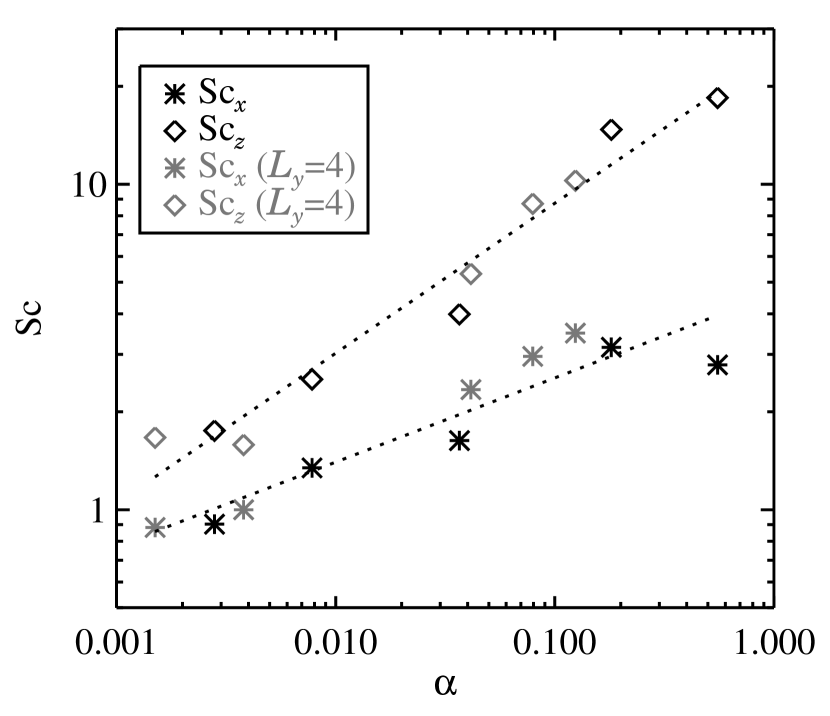
Figure 1: The Schmidt number plotted against the $\alpha$ value and the best power-law fit (dotted lines). The best fit has ${\rm Sc}_{x}=4.6\alpha^{0.26}$ and ${\rm Sc}_{z}=25.3\alpha^{0.46}$.

For each value of the imposed magnetic field we have measured the $\alpha$-value from the Reynolds and Maxwell stress tensors (see Table 1). The $\alpha$-value grows approximately exponentially with $B_{0}$. An $\alpha$-value close to unity can be reached already for $B_{0}=0.07$ (corresponding to $\beta\simeq 400$). A similar investigation into the dependence of $\alpha$ on an imposed vertical field was undertaken by Hawley et al. (1995). Comparing with Table 1 in that work, one sees that there is a relatively good agreement between those results and ours. Magnetorotational instability with an imposed vertical field develops into a “channel” solution (Hawley & Balbus, 1992; Goodman & Xu, 1994; Steinacker & Henning, 2001), characterised by the transfer of the most unstable MRI mode to the the largest scale of the simulation box and the subsequent decay of this large scale mode (Sano & Inutsuka, 2001). Sufficiently strong vertical fields can even cause stratified discs to break up altogether (Miller & Stone, 2000). The creation and destruction of the unstable channel solution gives significant temporal fluctuations in the measured stresses, evident in the standard deviation of the turbulent viscosity in Table 1 (see also Fig. 1 of Sano & Inutsuka, 2001).

For measuring the turbulent diffusion coefficient we consider the logarithmic number density of the dust particles averaged from $10$ to $20$ orbits. We have chosen to calculate the diffusion coefficient directly from this average state, rather than calculating it from the instantaneous dust density at a given time $t$, because large-scale advection flow only works as diffusion when averaged over sufficiently long times. The average dust density was found to be in excellent agreement with the cosine distribution of equation (9) with a deviation from a perfect cosine of less than $5\%$ for all simulations. Thus diffusion is a good description of the turbulent transport over long time-scales. This is partly due to the fact that we consider diffusion at the largest scale of the flow, i.e. at a scale that is similar to or larger than the energy injection scale of the MRI. Diffusion over length scales that are smaller than the energy injection scale should be weaker, because dust density concentrations at small length scales are not stretched by the full velocity amplitude of the larger scales, but only by the velocity difference that the larger scales exert over the much narrower dust concentration. The $\exp(\cos)$ equilibrium state for the dust density, however, has almost all of its power at the largest scale of the simulation box, so any scale-dependency of the diffusion coefficient should not have any influence on the equilibrium state (the fact that the logarithmic dust density in the equilibrium state is a cosine supports this).

The measured turbulent diffusion coefficients are written in Table 1. It is evident that the turbulent diffusion coefficient does not increase as fast with increasing vertical field as the turbulent viscosity does. In Fig. 1 we plot the vertical and radial Schmidt numbers as a function of $\alpha$. Both Schmidt numbers approximately follow a power law with $\alpha$. Making a best-fit power law, we find the empirical connections

$${\rm Sc}_{x} = \,\,\,4.6\alpha^{0.26}\,,$$ (10)

$${\rm Sc}_{z} = 25.3\alpha^{0.46}\,.$$ (11)

Considering the two box sizes individually (black and grey symbols in Fig. 1), the radial Schmidt number is seen to rise slightly faster with increasing $\alpha$ in the case of the elongated box with $L_{y}=4$, whereas the vertical Schmidt number follows a trend that is independent of the box size. In ideal MHD simulations with $\beta=400$, CSP05 find a radial Schmidt number of around $10$. Using a similar value for $\beta$, we find that the radial Schmidt number rises from unity in the case of no external field to $\sim 3-4$ when $\beta\simeq 400$. This may explain at least part of the discrepancy between the results by CSP05 and JK05. The box size used in CSP05 is $1.0\times 6.28\times 1.0$, and is thus comparable to our elongated box. We have tried with $L_{y}=6.28$ as well, but found no significant difference in the results.

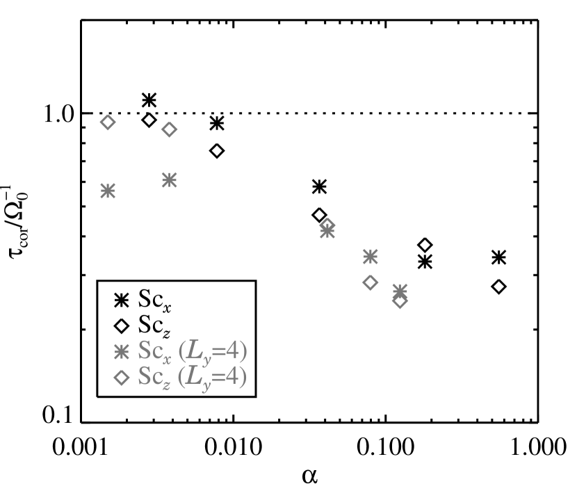
Figure 2: The correlation time of the turbulent mixing coefficients versus the $\alpha$-value. The correlation times fall significantly with increasing $\alpha$.

It is interesting to note that Fromang & Papaloizou (2006) have an $\alpha$-value of $0.015$ and a vertical Schmidt number of $2.8$. That fits almost perfectly in Fig. 1. Since Fromang & Papaloizou (2006) do not have an imposed vertical field in their simulations, this may mean that the rise in Schmidt number with $\alpha$ is something fundamental and not only an effect of the imposed magnetic field, although further investigations would have to be done to explore this connection in more detail.

4.1 Correlation times

One can express the diffusion coefficient caused by the scale $k$ of a turbulent flow as $D_{k}=u_{k}\ell_{k}$. Here $u_{k}$ is the velocity amplitude of that scale and $\ell_{k}$ is the typical length-scale over which a turbulent feature transports before dissolving. The advection length $\ell_{k}$ can be approximated by $\ell_{k}=u_{k}t_{k}$, where $t_{k}$ is the correlation time, or life time, of a turbulent structure. Taking now an average (and weighted) correlation time $\tau_{\rm cor}$ of all the scales, one gets the mixing length expression for the diffusion coefficient in direction $i$,

$$D_{i}^{({\rm t})}=\tau_{\rm cor}u_{i}^{2}\,,$$ (12)

valid for Fickian diffusion (for the validity of Fickian diffusion see Brandenburg et al., 2004). Here the Mach number, $\sqrt{u_{i}^{2}}/c_{\rm s}$, is the root-mean-square velocity fluctuation in real space. The diffusion coefficient should thus scale roughly with Mach number squared. We plot the correlation times, calculated from equation (12), of $\delta_{x}$ and $\delta_{z}$ versus the $\alpha$-value of the flow in Fig. 2. The correlation time of the turbulent diffusion coefficients falls steeply with increasing $\alpha$-value, so even though the Mach number of the flow increases, the time a given turbulent structure has for transporting the dust becomes shorter and shorter. Since the correlation times of radial and vertical diffusion have approximately the same dependence on $\alpha$, the ratio of the diffusion coefficients can be expressed as $\delta_{x}/\delta_{z}=({\rm Ma}_{x}/{\rm Ma}_{z})^{2}$. The anisotropy in the diffusion coefficient in favour of the radial direction is then mostly an effect of the anisotropy between the radial and vertical Mach numbers.

5 Summary

In this letter we report that the Schmidt number of magnetorotational turbulence depends strongly on the value of an imposed vertical magnetic field. For large values of the vertical field, the relative strength of the turbulent diffusion falls with respect to the turbulent viscosity. This could explain part of the discrepancy between measurements of the radial turbulent diffusion coefficient in magnetorotational without an imposed field (Johansen & Klahr, 2005) and with an imposed field (Carballido et al., 2005).

References

- Balbus & Hawley (1991) Balbus, S. A., & Hawley, J. F. 1991, ApJ, 376, 21
- Barge & Sommeria (1995) Barge, P., & Sommeria, J. 1995, A&A, 295, L1
- Bourke et al. (2001) Bourke T. L., Myers P. C., Robinson G., & Hyland A. R. 2001, ApJ, 554, 916
- Brandenburg et al. (1995) Brandenburg, A., Nordlund, Å., Stein, R.F., & Torkelsson, U. 1995, ApJ, 446, 741
- Brandenburg (2003) Brandenburg, A. 2003, in Advances in nonlinear dynamos (The Fluid Mechanics of Astrophysics and Geophysics, Vol. 9), ed. A. Ferriz-Mas & M. Núñez (Taylor & Francis, London and New York), 269-344
- Brandenburg et al. (2004) Brandenburg, A., Käpylä, P. J., & Mohammed, A. 2004, Physics of Fluids, 16, 1020
- Camenzind (1990) Camenzind, M. 1990, Reviews of Modern Astronomy, 3, 234
- Carballido et al. (2005) Carballido, A., Stone, J. M., & Pringle, J. E. 2005, MNRAS, 358, 1055
- Dominik et al. (2006) Dominik, C., Blum, J., Cuzzi, J., & Wurm, G. 2006, in Protostars and Planets V (astro-ph/0602617)
- Dullemond et al. (2006) Dullemond, C. P., Apai, D., & Walch, S. 2006, ApJ, in press
- Fendt & Elstner (1999) Fendt, C., & Elstner, D. 1999, A&A, 349, L61
- Fendt & Elstner (2000) Fendt, C., & Elstner, D. 2000, A&A, 363, 208
- Fleming & Stone (2003) Fleming, T., & Stone, J. M. 2003, ApJ, 585, 908
- Fromang & Papaloizou (2006) Fromang, S., & Papaloizou, J. 2006, astro-ph/0603153
- Gammie (1996) Gammie, C. F. 1996, ApJ, 457, 355
- Goldreich & Tremaine (1978) Goldreich, P. & Tremaine, S. 1978, ApJ, 222, 850
- Goodman & Xu (1994) Goodman, J., & Xu, G. 1994, ApJ, 432, 213
- Haugen et al. (2004) Haugen, N. E. L., Brandenburg, A., & Mee, A. J. 2004, MNRAS, 353, 94
- Hawley & Balbus (1992) Hawley, J. F., & Balbus, S. A. 1992, ApJ, 400, 595
- Hawley et al. (1995) Hawley, J. F., Gammie, C. F., & Balbus, S. A. 1995, ApJ, 440, 742
- Ilgner et al. (2004) Ilgner, M., Henning, T., Markwick, A. J., & Millar, T. J. 2004, A&A, 415, 643
- Ilgner & Nelson (2006) Ilgner M., & Nelson R. P. 2006, A&A, 445, 223
- Johansen & Klahr (2005) Johansen, A., & Klahr, H. 2005, ApJ, 634, 1353
- Königl (1991) Königl, A. 1991, ApJL, 370, L39
- Küker et al. (2003) Küker, M., Henning, T., & Rüdiger, G. 2003, ApJ, 589, 397
- Miller & Stone (1997) Miller, K. A., & Stone, J. M. 1997, ApJ, 489, 890
- Miller & Stone (2000) Miller, K. A., & Stone, J. M. 2000, ApJ, 534, 398
- Rodmann et al. (2006) Rodmann, J., Henning, T., Chandler, C. J., Mundy, L. G., & Wilner, D. J. 2006, A&A, 446, 211
- Sano & Inutsuka (2001) Sano, T., & Inutsuka, S.-i. 2001, ApJL, 561, L179
- Sano et al. (2004) Sano, T., Inutsuka, S.-i., Turner, N. J., & Stone, J. M. 2004, ApJ, 605, 321
- Semenov et al. (2006) Semenov, D., Wiebe, D., & Henning, T. 2006, submitted to ApJ
- Shakura & Sunyaev (1973) Shakura, N. I., & Sunyaev, R. A. 1973, A&A, 24, 337
- Shu et al. (1994) Shu, F., Najita, J., Ostriker, E., Wilkin, F., Ruden, S., & Lizano, S. 1994, ApJ, 429, 781
- Steinacker & Henning (2001) Steinacker, A., & Henning, T. 2001, ApJ, 554, 514
- Turner et al. (2006) Turner, N. J., Willacy, K., Bryden, G., & Yorke, H. W. 2006, ApJ, 639, 1218
- Vlemmings et al. (2006) Vlemmings, W. H. T., Diamond, P. J., Imai, H. 2006, Nature, 440, 58
- Weidenschilling (1977) Weidenschilling, S. J. 1977, MNRAS, 180, 57
- Willacy et al. (2006) Willacy, K., Langer, W. D., Allen, M., & Bryden, G. 2006, astro-ph/0603103