A large stellar evolution database for population synthesis studies. II. Stellar models and isochrones for an $\alpha-$enhanced metal distribution

Abstract

We present a large, new set of stellar evolution models and isochrones for an $\alpha$-enhanced metal distribution typical of Galactic halo and bulge stars; it represents a homogeneous extension of our stellar model library for a scaled-solar metal distribution already presented in Pietrinferni et al. (2004). The effect of the $\alpha-$element enhancement has been properly taken into account in the nuclear network, opacity, equation of state and, for the first time, the bolometric corrections, and color transformations. This allows us to avoid the inconsistent use - common to all $\alpha$-enhanced model libraries currently available - of scaled-solar bolometric corrections and color transformations for $\alpha$-enhanced models and isochrones. We show how bolometric corrections to magnitudes obtained for the $U,B$ portion of stellar spectra (i.e. not only the Johnson-Cousins filters but also Strömgren $u,b$ magnitudes) for $T_{eff}\leq 6500$ K, are significantly affected by the metal mixture, especially at the higher metallicities.

Our models cover both an extended mass range (between $0.5M_{\odot}$ to $10M_{\odot}$, with a fine mass spacing) and a broad metallicity range, including 11 values of the metal mass fraction $Z$, corresponding to the range $-2.6\leq[Fe/H]\leq 0.05$. The initial He mass fraction is $Y$=0.245 for the most metal-poor models and increases with $Z$ according to $\Delta Y/\Delta Z$=1.4, to reproduce the initial solar He obtained from the calibration of the solar model. Models with and without the inclusion of overshoot from the convective cores during the central H burning phase are provided, as well as models with different mass loss efficiencies.

We also provide complete sets of evolutionary models for low-mass, He-burning stellar structures covering the whole metallicity range, to enable synthetic horizontal branch simulations.

We compare our database with several widely used stellar model libraries from different authors, as well as with various observed color magnitude and color-color diagrams (Johnson-Cousins $BVI$ and near infrared magnitudes, Strömgren colors) of Galactic field stars and globular clusters. We also test our isochrones comparing integrated optical colors and Surface Brightness Fluctuation magnitudes with selected globular cluster data. We find a general satisfactory agreement with the empirical constraints.

This database, used in combination with our scaled-solar model library, is a valuable tool for investigating both Galactic and extra-galactic simple and composite stellar populations, using stellar population synthesis techniques.

1 Introduction

Large libraries of stellar models and isochrones covering wide ranges of age and metallicities are an essential tool to investigate the properties of resolved and unresolved stellar populations. We have recently published (Pietrinferni et al. 2004, hereafter Paper I) an extended database of scaled-solar stellar evolution models and isochrones that is very well suited to accomplish this goal.

It is however well known that the scaled-solar metal mixture is not universal. In particular, observations of metal abundance ratios in the Galaxy (i.e., Ryan, Norris & Bessel 1991; Carney 1996; Gratton, Sneden & Carretta 2004; Sneden 2004;) have shown that [$\alpha$/Fe] (where with $\alpha$ we denote collectively the so called $\alpha$-elements O, Ne, Mg, Si, S, Ar, Ca and Ti) is larger than zero in Population II field stars, Galactic globular clusters (see, e.g., Carney 1996) and in Galactic bulge stars (see, e.g., McWilliam & Rich 2004) that is, the abundance ratio $\alpha$/Fe is larger than the solar counterpart. Typical values of [$\alpha$/Fe] in the Galactic halo are $\sim 0.3-0.4$ dex. In addition, also stellar populations in elliptical galaxies appear to have formed with a metal mixture characterized by [$\alpha$/Fe]$>$0 (see, i.e., Worthey, Faber & Gonzalez 1992; Tantalo, Chiosi & Bressan, 1998; Trager et al. 2000)

From a theoretical point of view, the first extended set of isochrones accounting for the enhancement of oxygen was published by Bergbusch & Vandenberg (1992) (and oxygen-enhanced Horizontal Branch models by Dorman 1992); the enhancement of all $\alpha$-element was exhaustively addressed by Salaris, Chieffi & Straniero (1993) in the regime of low mass, metal poor objects, while Weiss, Peletier & Matteucci (1995) studied the high metallicity regime. An important and useful property of $\alpha$-enhanced models shown by Salaris et al. (1993) is that, for $\alpha$-enhanced mixtures that satisfy the constraint [(C+N+O+Ne)/(Mg+Si+S+Ca+Fe)]=0 (as for example in case of a constant enhancement of all $\alpha$ elements) low mass stellar models computed with an [$\alpha$/Fe]$>$0 metal distribution are equivalent to scaled-solar ones with the same global metal content $Z$ (see also Chaboyer, Sarajedini & Demarque 1992). This property breaks down at values of Z larger than about Z=0.002 (see, e.g., Weiss et al. 1995, VandenBerg & Irwin 1997, Salaris & Weiss 1998, Salasnich et al. 2000, VandenBerg et al. 2000, Kim et al. 2002).

These theoretical results have been obtained neglecting the effect of an $\alpha$-enhancement on the bolometric corrections to be applied to the theoretical isochrones. Very recently, Cassisi et al. (2004) addressed this issue for the first time, showing that broadband colors involving the $UB$ part of the spectrum are affected by the enhancement of the $\alpha$-element, whereas redder wavelength bands are not affected. Both $(B-V)$ and $(U-B)$ colors appear bluer than the scaled-solar ones at either the same [M/H] or the same [Fe/H], the difference increases with increasing metal content and/or decreasing effective temperature. The best way to mimic $\alpha$-enhanced color transformations is to use scaled-solar ones with the same [Fe/H], but this equivalence breaks down when the iron content increases above [Fe/H]$\sim-$1.6. These differences are mainly due to the enhancement of Mg with lower contributions from the enhancement of Si and O.

The use of scaled-solar isochrones to mimic their $\alpha$-enhanced counterpart is not valid over the full metallicity range where ratios [$\alpha$/Fe]$>$0 have been observed, so that it is important to compute models and isochrones that include appropriate values of [$\alpha$/Fe]. In the last years Salaris & Weiss (1998), VandenBerg et al. (2000), VandenBerg (2000), Salasnich et al. (2000), Kim et al. (2002) have published sets of $\alpha$-enhanced isochrones that cover to different degrees the age and metallicity parameter range. None of these sets adopt appropriate $\alpha$-enhanced bolometric corrections and color transformations.

In this paper we enlarge the parameter space covered by the model and isochrone library presented in Paper I, by extending our computations to an $\alpha$-enhanced metal distribution, where the [$\alpha$/Fe] value is consistent with observations of the Galactic halo population. This new library covers exactly the same $Y,Z$ space, and the same mass ranges of our scaled-solar one presented in Paper I, and it has been computed with the same stellar evolution code and homogeneous physical inputs. It includes models computed both with and without overshooting from the convective cores, two different choices for the efficiency of mass loss and, for the first time, appropriate $\alpha$-enhanced color transformations and bolometric corrections for both the low- and high $Z$ regimes.

The paper is organized as follows: § 2 briefly summarizes the adopted physical inputs, while the model library is presented in § 3. Comparisons with widely used isochrone databases, and with selected empirical constraints are discussed in § 4, and § 5, respectively. A summary and final remarks follow in § 6.

2 Input physics and color transformations

We used the same stellar evolution code as in Paper I, and the reader is referred to this paper for more information. Here we just describe the new chemical and physical inputs necessary for the computation of the $\alpha$-enhanced library. The adopted $\alpha$-enhanced mixture is the same as in the models by Salaris, Degl’Innocenti & Weiss (1997) and Salaris & Weiss (1998) and it is reported in Table 1. The $\alpha$-elements have been enhanced with respect to the Grevesse & Noels (1993) solar metal distribution (that is the heavy element distribution used in Paper I) by variable factors, following mainly the results by Ryan et al. (1991) about field Population II stars. The overall average enhancement is [$\alpha$/Fe]$\sim$0.4. This $\alpha$-enhanced distribution has been used in the nuclear network, the radiative (Iglesias & Rogers 1996, Alexander & Ferguson 1994) and conductive opacities (Potekhin et al. 1999) and the equation of state.

Although our stellar evolution code can account for the atomic diffusion of helium and heavy elements, we decided to neglect this process in our model grid computation. As largely discussed in Paper I, we have accounted for atomic diffusion when computing the standard solar models. This choice allowed us to properly calibrate the mixing length (see below) and to estimate the initial solar chemical composition. Although in the Sun atomic diffusion is essentially fully efficient, spectroscopic observations of stars in Galactic globular clusters or field halo stars (see section II of Paper I) point to a drastically reduced efficiency of this process, due possibly to the counteracting effect of rotationally induced mixing processes. This evidence raises the possibility that the almost uninhibited efficiency of diffusion found in the Sun might not be an occurrence common to all stars.

Superadiabatic convection is treated according to the Cox & Giuli (1968) formalism of the mixing length theory (Böhm-Vitense 1958) and the mixing length value is, as in the case of the scaled-solar models, equal to 1.913, as obtained from a calibration of the solar model (see Paper I for details).

All models include mass loss using the Reimers formula (Reimers 1975) with the free parameter $\eta$ set to two different values: 0.2 and 0.4.

We made the same assumptions as in Paper I regarding the treatment of convection at the border of convective core during the core H-burning phase of stars with total mass larger than $\sim 1.1M_{\odot}$. Two different values are adopted for the overshoot from the Schwarzschild convective boundary, namely $\lambda_{OV}=0$ and 0.2. With $\lambda_{OV}$ we denote the length - expressed as a fraction of the local pressure scale height - crossed by the convective cells in the stable region outside the Schwarzschild boundary. The amount of core overshoot is decreased in the same way as in Paper I, when the convective core size decreases to zero as a consequence of the decreasing total stellar mass. The treatment of convection in the core of central He-burning stars is exactly the same of Paper I. The possible occurrence of overshooting from the bottom of the convective envelopes has been neglected as in Paper I for the reasons discussed in that paper.

Finally, the theoretical tracks and isochrones have been transformed to various observational Color-Magnitude Diagrams (CMDs) using color-$T_{eff}$ transformations and bolometric corrections (that we will denote collectively as CT) obtained from an updated version of ATLAS9 model atmospheres (Castelli & Kurucz 2003). The scaled-solar and [$\alpha$/Fe]=0.4 CT have been described in Paper I and in Cassisi et al. (2004). In the latter paper a subset of the $\alpha$-enhanced CT has been used to investigate the impact of an $[\alpha/Fe]>0$ metal distribution on broadband colors. Grids of model atmospheres, energy distribution, color indices in the $UBVRIJKL$, Strömgren $uvby$ and Walraven photometric systems have been computed for $[Fe/H]$: $-2.5$, $-2.0$, $-1.5$, $-1.0$, $-0.5$, $0.0$, $+0.2$ and $+0.5$. For a more detailed discussion about the adopted passbands and the model atmosphere grid the reader is referred to Paper I and to Cassisi et al. (2004). Here we only add that the Strömgren colors used in this paper were computed according the prescriptions given by Relyea & Kurucz (1978).

3 The evolutionary tracks and isochrones

The grid of chemical compositions of our library covers 11 pairs of $Y,Z$ values, as listed in Table 2, ranging from $Z$=0.0001 to $Z$=0.04. They are the same $Y,Z$ values of our scaled-solar library, although the correspondence between $Z$ and [Fe/H] is different, due to the effect of the $\alpha$-enhancement. We wish to note that in the scaled-solar library presented in Paper I, the $Z=0.0006$ metallicity was originally missing; it has been added later, in order to improve the sampling of the low-metallicity regime. We have used $Y=0.245$ for the lowest metallicity, together with $dY/dZ\sim 1.4$ that allows to match the calibrated initial He abundance in the Sun.

We have used the same stellar mass range and sampling as in Paper I, to be consistent with the scaled-solar library, and to optimize the use of both sets of models in a stellar population synthesis code. For each chemical composition, we have computed the evolution of up to 41 different stellar masses, with a minimum mass equal to $0.50M_{\odot}$, and a maximum mass always equal to $10M_{\odot}$. We adopted a mass step of $\Delta{M}=0.1M_{\odot}$ (or lower) for masses below $2.5M_{\odot}$, $\Delta{M}=0.2M_{\odot}$ for masses in the range $2.5\leq{M/M_{\odot}}\leq 3.0$, and $\Delta{M}=0.5M_{\odot}$ for more massive models. Models less massive than $\sim 3M_{\odot}$ have been computed starting from the pre-MS phase, whereas the more massive ones have been computed starting from a chemically homogeneous configuration on the MS. All models, apart from the less massive ones whose central H-burning evolutionary times are longer than the Hubble time, have been evolved until the C ignition or after the first few thermal pulses along the Asymptotic Giant Branch (AGB) phase. We are already working to extend the evolution of low mass and intermediate mass stars up to the end of the thermal pulses along the AGB, using the synthetic AGB technique (see, e.g., Marigo, Bressan, & Chiosi 1996 and reference therein).

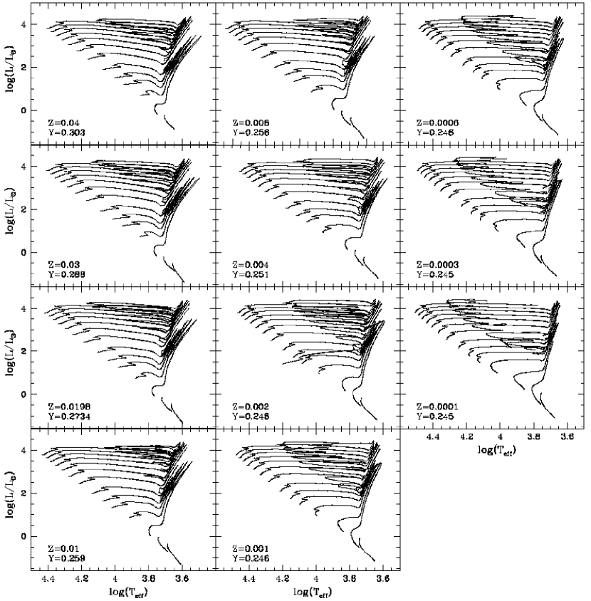
Figure 1: Selected evolutionary tracks for the 11 metallicities of our model grid.

In case of models undergoing a violent He flash at the Red Giant Branch (RGB) tip, we do not perform a detailed numerical computation of this phase, but we use the evolutionary values of both the He core mass, $M_{cHe}$, and the chemical profile at the RGB tip to compute the corresponding Zero Age Horizontal Branch (ZAHB) model (see Vandenberg et al. 2000 for a careful check of the validity of this approach). A subsample of the evolutionary tracks (models without convective overshoot and $\eta$=0.2) is shown in Fig. 1 for the entire chemical composition range.

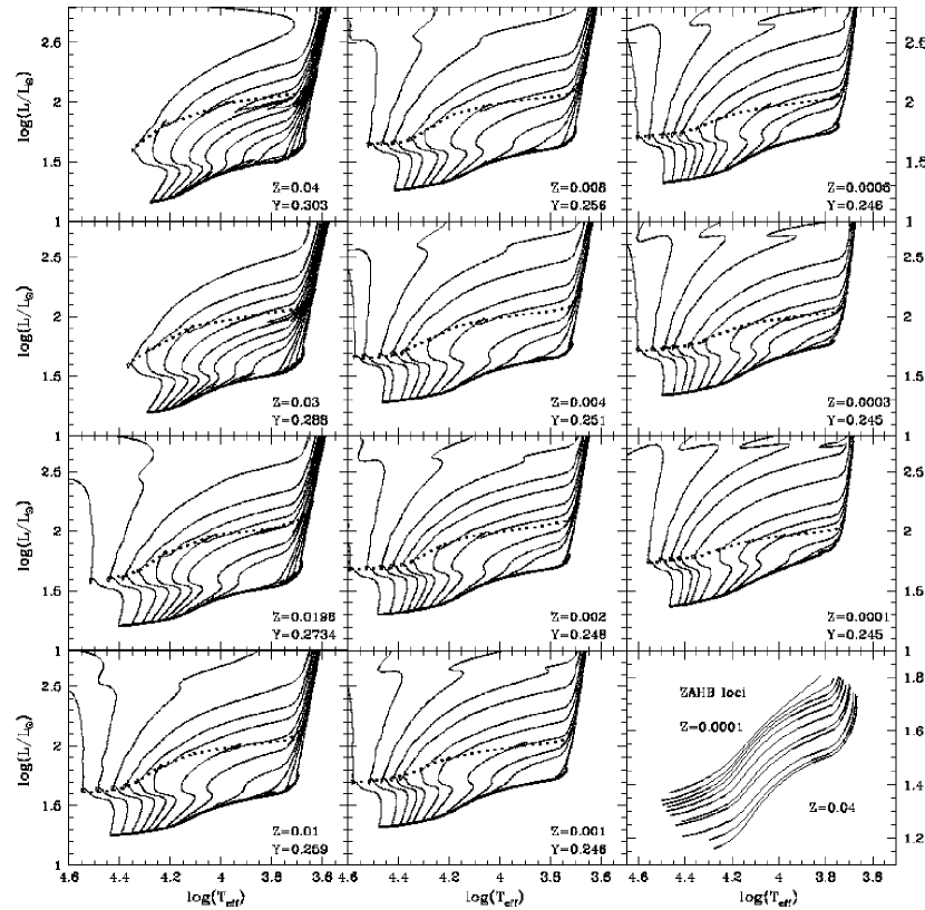
Figure 2: Additional HB evolutionary tracks suited for the computation of synthetic HB populations. The figure shows also the location of the ZAHB and central He exhaustion loci (dotted lines).

For each chemical composition, we have also computed an extended set of He burning models – that is, HB models in addition to the one obtained with our chosen mass loss law – with various different values of the total stellar mass after the RGB phase, using the fixed core mass and chemical profiles given by an RGB progenitor having an age (at the RGB tip) of $\sim 13$Gyr. These models allow one to compute the CMD of synthetic HB populations, including an arbitrary spread of the amount of mass lost along the RGB phase (typical of Galactic globular clusters). The RGB progenitor of these additional HB models has a mass typically equal to $0.8M_{\odot}$ at the lowest metallicities, increasing up to 1.0$M_{\odot}$ for the more metal-rich compositions. Table 3 lists the main characteristics of these HB models, namely, the He core mass at the ZAHB, the envelope He content, the total mass, luminosity and absolute visual magnitude of the object whose ZAHB location is at $\log{T_{eff}}=3.85$ - taken as rapresentative of the mean temperature inside the RR Lyrae instability strip. For these additional He-burning computations we have employed a fine mass spacing, and more than 30 HB models have been computed for each chemical composition. A subset of these models is displayed in Fig. 2. The same figure shows also the location of the ZAHB and central He-exhaustion loci.

All the post-ZAHB computations have been extended either to the onset of thermal pulses for more massive models, or until the luminosity along the white dwarf cooling sequence has decreased down to $\log(L/L_{\odot})\sim-2.5$ for less massive objects. They allow a detailed investigation of the various evolutionary paths that follow the exhaustion of the central He burning.

The individual evolutionary tracks have been reduced to the same number of points, to facilitate the computation of isochrones and their use in a population synthesis code. Along each evolutionary track some characteristic homologous points (key points – KPs) corresponding to well-defined evolutionary phases have been identified. The choice and number of KPs had to fulfill two conditions: 1) all main evolutionary phases have to be properly accounted for; 2) the number of KPs has to be large enough to allow a suitable sampling of the track morphology, even for fast evolutionary phases. The second condition requires also that the number of points between two consecutive KPs has to be properly chosen.

For a careful description of the adopted KPs we refer to Paper I. In the original version of the database, we adopted 14 key stages along the evolutionary tracks (see Paper I). For our actual stellar models library, we have accounted for 16 key stages along the evolutionary track to obtain a more accurate sampling of the track morphology (we thank A. Dolphin for pointing out to us the need of a more accurate sampling of the RGB bump region). Of course all evolutionary tracks for the scaled-solar metal distribution have been re-reduced by accounting for the same 16 KPs. The whole set of evolutionary computations (but the additional HB models discussed above) have been used to compute isochrones for a large age range, namely, from 30 Myr up to 16 Gyr (older isochrones can also be computed), from the Zero Age Main Sequence (ZAMS) up to the first thermal pulse along the AGB or to the C ignition .

The entire library of evolutionary tracks and isochrones is available upon request to one of the authors or can be retrieved at the WEB site http://www.te.astro.it/BASTI/index.php.

At the same URL site, we have made available a World Wide Web interface (more details will be provided in a forthcoming paper, D. Cordier et al. 2006 in preparation) that allows a user to compute isochrones, evolutionary tracks and luminosity functions for any specified stellar mass, chemical composition, age. Detailed tables displaying the relevant evolutionary features for all computed tracks are also available.

The files containing the isochrones provide at each point (2000 points in total) the initial value of the evolving mass, the actual mass value (in principle different, due to the effect of mass loss), $\log(L/L_{\odot})$, $\log{T_{eff}}$, and absolute magnitudes in different photometric systems (see the discussion in the next section).

These isochrones - as well as those for a scaled-solar metal distribution - can be used as input data for our fortran code $SYNTHETICMAN(ager)$ that we have written in order to compute synthetic CMDs, integrated colors and integrated magnitudes of a generic stellar population with an arbitrarily chosen star formation rate and age metallicity relation. A presentation of this code can be found in Paper I and it will not be repeated here. In the near future, we will allow users to run this code through a P.E.R.L based, Web interface. In addition to a chosen Star Formation History the user will be free to fix various other parameters like photometric and spectroscopic errors, color excess, fraction of unresolved binaries, geometrical depth of the population. The access to this tool will require registration, the results being sent to the user by e-mail.

3.1 The impact of an $\alpha-$enhanced metal distribution on HB structures

Before closing this section, we wish to briefly discuss the effect of an $\alpha$-enhanced metal distribution on the HB evolution. Although the effect of $\alpha-$enhanced mixtures on H-burning models is well known and widely discussed in the literature (see the references in the introduction) the behavior of $\alpha$-enhanced He-burning models compared to their scaled-solar counterpart has been investigated only by Salaris et al. (1993) and VandenBerg et al. (2000), although the latter studied the effect on the ZAHB location only. An earlier investigation by Bencivenni et al. (1989) did not take into account the effect of an [$\alpha$/Fe]$>$0 mixture on the HB progenitor evolution.

Figure 3 shows the comparison between an $\alpha-$enhanced HB model in the instability strip and the corresponding scaled-solar one at fixed total mass for various values of $Z$. At fixed total mass and global metallicity, $\alpha-$enhanced HB models appear brighter and hotter than the scaled-solar ones, and in particular for values of $Z$ larger than $\sim$0.002. At $Z=10^{-4}$, the luminosity difference is negligible, $\Delta\log(L/L_{\odot})\approx 0.004$, while at $Z=0.002$, $\Delta\log(L/L_{\odot})\approx 0.02$. These differences increase to $\sim 0.03$ and $\sim 0.05$ at $Z=0.0198$ and $Z$=0.04, respectively. These results about the brighter and hotter location of $\alpha$-enhanced HB models in the instability strip agree well with the findings by Salaris et al. (1993) and VandenBerg et al. (2000). For $Z\geq$0.002 the $\alpha-$enhanced ZAHB models have a He core mass lower than the scaled-solar case by only $\sim 0.001M_{\odot}$ (regardless of the metallicity) and an envelope He abundance essentially equal to or lower by at most $\Delta Y\sim$0.001; this means that the difference in the ZAHB location and HB evolution is due to the increased efficiency of the CNO-cycle in the H-burning shell with respect to the core burning in models with an [$\alpha$/Fe]$>$0 distribution.

As for the lifetime along the HB phase for a given $Z$, we find that it is only marginally affected by the use of an $\alpha-$enhanced metal distribution, irrespective of the precise value of $Z$. The central He-burning lifetime decreases compared to the scaled-solar mixture by a negligible $\sim 1$% at low metallicity, and about $\sim 4$% at the highest metallicity of our model grid. The same change holds for the AGB lifetime up to the thermal pulse phase. This has the important consequence that the theoretical calibrations of the $R_{2}$ parameter (number ratio of AGB stars to HB stars; see e.g. Caputo et al. 1989) is not affected by the adopted metal distribution. This parameter is very important for its sensitivity to the extension of the convective cores during the central He-burning phase, and is used to assess the efficiency of the breathing pulses at the exhaustion of the central He.

A further important evolutionary feature is the brightness of the AGB clump, marking the ignition of the He-burning in a shell. We have verified that the brightness of the AGB clump is slightly larger with respect the scaled-solar case, the difference tracking the luminosity difference of the ZAHB models. This implies that the brightness difference between the ZAHB and the AGB clump is preserved when passing from a scaled-solar mixture to an $\alpha-$enhanced one with the same $Z$, for any value of $Z$.

3.2 $\alpha-$enhanced vs scaled-solar transformations

Cassisi et al. (2004) analized the impact of $\alpha$-enhanced CT in the $UBVRIJHKL$ filters, for the metallicity regime of Galactic globular clusters, and their results have been already summarized in the introduction. Here we extend the analysis to higher metallicities. Figure 4 shows the comparison between 12 Gyr old $\alpha$-enhanced isochrones and ZAHB for $Z$=0.0198 and $Z$=0.04 in various CMDs, using different CT. More in detail, we used the appropriate $\alpha$-enhanced CT, a scaled-solar CT with the same [Fe/H] of the isochrone, and a scaled-solar CT with the same [M/H] (total metallicity) of the isochrone.

We find (in agreement with the results at lower $Z$) that the $V$ magnitudes are hardly affected, whereas the $(U-B)$ and $(B-V)$ colors predicted by the scaled-solar CT with the same [M/H] of the isochrone are systematically redder along the whole isochrone. Differences are smaller when considering scaled-solar CT with the same [Fe/H] of the isochrone. This occurrence means that it is the abundance of Fe and of all other scaled-solar elements that contribute mostly to the observed color, although not completely, given the difference with the appropriate CT – but they still reach up to $\sim$ 0.1 mag along a large fraction of the isochrone. This is due to the effect of the $\alpha$-enhancement in the wavelength range of the $U$ and $B$ filter (see discussion in Cassisi et al. 2004).

A different approach to mimic $\alpha$-enhanced CT with scaled solar ones, is to use scaled-solar CT with the same [$\alpha$/H] ratio of the [$\alpha$/Fe]$>$0 distribution. So doing, one assumes that it is essentially the abundance of $\alpha$-elements that affects the colors. The data in Figure 4 show that this choice is much less accurate, since it corresponds to a scaled-solar CT with a [M/H] value 0.4 dex larger that the actual one, that yields even redder colors.

Interestingly, the $(V-I)$ color is also affected by the CT choice at high metallicities and low temperatures. The two scaled-solar CT produce colors this time systematically bluer than the appropriate $\alpha$-enhanced CT, the CT with the same [Fe/H] of the isochrone giving the worst results. On the basis of our previous discussion it is clear that in this case a scaled-solar CT with the same [$\alpha$/H] ratio of the isochrone would provide colors closer to the appropriate ones. This suggests that the abundance of the $\alpha$-elements (or at least some of them) starts to dominate the CT in this wavelength range for solar and super-solar metallicities, and low temperatures.

Figure 5 shows another comparison of CT applied to a 12 Gyr old $\alpha$-enhanced isochrone at various $Z$, considering the appropriate $\alpha$-enhanced transformations and the same two choices for the scaled-solar CT as in Fig. 4, this time involving the Strömgren filters. The Strömgren $u$, $v$ and $b$ filters are located in the wavelength range of the Johnson $U$ and $B$ bands; therefore one expects a relevant influence of the $\alpha$-elements on, for example, the $[c_{1},b-y]$ color-color plane, used to estimate ages of star clusters and field stars, independently of the knowledge of their distance.

The use of different CT affects strongly the isochrone morphology in this plane, as shown clearly by Fig. 5. The effect is appreciable from $Z\sim$0.001 and is, as expected, larger at larger metallicities. The sections of the isochrone that are more affected are, as for the case of Johnson colors, the RGB and the lower MS. Again, scaled-solar CT at the same [Fe/H] of the appropriate ones give a better approximation to the real CT, apart from the highest $Z$, where differences are huge for both scaled solar CT. In Fig. 6 we show isochrones for various ages and $Z=0.004$, transformed to the $[c_{1},b-y]$ plane using the same three choices of CT. One can notice that the 12 Gyr old isochrone transformed using the scaled-solar CT with the appropriate [Fe/H] matches well Turn Off (TO) and subgiant branch obtained with the appropriate colors. On the contrary, using scaled-solar CT with the same [M/H] of the $\alpha$-enhanced ones causes not only a change of the morphology of the lower MS and the RGB, but also a shift of both $c_{1}$ and $b-y$ of the upper MS, TO and subgiant region; this induces systematic errors in both the age and reddening determined from isochrone fitting.

4 Comparison with existing databases

In this section we discuss the comparison in the H-R diagram of selected isochrones with similar predicitions from the databases by Salasnich et al. (2000), Salaris & Weiss (1998), VandenBerg et al. (2000) and Kim et al. (2002).

These grids of models are computed employing some different choices of the physical inputs (the source of the opacities is quite often the same, but equation of state, nuclear reaction rates, boundary conditions and neutrino energy loss rates are often different) and also the chemical compositions are often different. We perform the comparison on the theoretical H-R diagram, thus bypassing the additional degree of freedom introduced by the choice of the color transformations. In each comparison we have selected chemical compositions as close as possible to our choices. It is important to notice that Kim et al (2002) models do include He diffusion, and therefore their isochrones for old ages (above a few Gyr) are affected by the efficiency of this process.

Figure 7 shows the comparison in the H-R diagram of a $Z=0.008$, 12 Gyr old isochrone from Salaris & Weiss (1998 - hereafter SW98) with our own isochrone with the same age and metallicity, from the ZAMS to the TRGB. The ZAHBs are also displayed. Metal mixture and opacities are exactly the same in two models, and also the initial He mass fraction is practically identical ($Y=0.254$ in SW98 models, compared to our adopted value of $Y=0.256$).

There are some differences in the luminosities of the ZAHB and to a lesser extent the TO of the two isochrones. The ZAHB from SW98 is brighter by $\Delta\log(L/L_{\odot})\sim$0.03-0.04, whereas the TO is fainter by $\Delta\log(L/L_{\odot})\sim$0.02. Effective temperatures along the MS are in good agreement, but the temperature at the TO region and along large part of the RGB of our isochrones is hotter by about 70 K and $\sim$50 K, respectively.

A similar comparison but with a 12 Gyr old $\alpha$-enhanced isochrones by Salasnich et al. (2000 - hereafter S00) is displayed in Fig. 8. S00 models have also been computed using the same metal mixture and opacities employed in our own calculations; at $Z=0.008$ the initial He abundance of their models ($Y=0.250$) is close enough to ours, to provide a meaningful comparison. As for our models, we display the ZAHB and the full 12 Gyr isochrone computed with the Reimers parameter $\eta$=0.2.

The effective temperatures agree well along MS and RGB for $T_{eff}$ larger than about 5000 K. At lower temperatures the S00 isochrone is systematically hotter. The ZAHB luminosity of S00 models is fainter by $\Delta\log(L/L_{\odot})\sim$0.04.

Given that S00 provide also $\alpha$-enhanced isochrones for low ages, we show in Fig. 9 a comparison of 500 Myr old isochrones. Current and S00 isochrone include overshooting from the convective core, albeit with different prescriptions. The TO region of our isochrone is brighter and hotter than S00 counterpart. This is consistent with the result of a similar comparison between our 500 Myr scaled-solar isochrone of solar metallicity and the corresponding one from Girardi et al. (2000), that should be computed with physical prescriptions very similar to S00. As we remarked in Paper I, the interplay between the different treatment of the core overshooting and some different input physics should play a major role in causing this difference. As for the scaled solar case our He burning phase is brighter than S00 one, but the post-MS effective temperatures of our isochrones are slightly cooler than S00, whereas in the scaled solar case they were hotter.

Figure 10 shows the comparison with a 12 Gyr old isochrone by VandenBerg et al. (2000) for $Z$=0.001 and $Z$=0.01. Although the selected $Z$ is the same of our isochrones, there exists some difference at the level of 0.01 in the initial He mass fraction, and the average $\alpha-$enhancement of our models is equal to 0.4 dex, whereas the Vandenberg et al. (2000) isochrones displayed in this comparison have [$\alpha$/Fe]=0.3, all $\alpha$-element being enhanced by the same amount.

Bearing in mind these differences between the two data sets, one notices that at $Z=0.001$ the MS almost completely overlap, whereas the TO of our isochrone is slightly brighter, by $\Delta\log(L/L_{\odot})\sim 0.005$ and $\sim 80$ K hotter. Along the RGB our isochrone is hotter by about 140 K, a difference larger than what we found in the case of the scaled-solar models compared in Paper I. This occurrence cannot be attributed to a combination of different EOS and solar mixing-length calibration, since we found a very good agreement for scaled-solar RGBs. Perhaps, it is mainly an effect due to the different $\alpha-$element enhancement and mixture and, to a lesser extent, the higher initial He content of our models. The brightness difference at $\log(T_{eff})=3.85$ along the ZAHB - taken as representative of the mean effective temperature of the RR Lyrae instability strip - is of the order of $\Delta\log(L/L_{\odot})\sim 0.04$.

The differences between the two sets of isochrones increase for increasing $Z$. At $Z=0.01$ the TO of our isochrone is brighter by $\Delta\log(L/L_{\odot})\sim 0.009$ and $\sim 140$ K hotter. Our RGB effective temperature is hotter by $\sim 170$ K, while the brightness difference at the RR Lyrae instability strip is equal to $\Delta\log(L/L_{\odot})\sim 0.05$.

Finally, we show in Fig. 11 a comparison with the $\alpha$-enhanced isochrones by Kim et al. (2002), with [$\alpha$/Fe]=0.3, $Z$=0.02 and $Y$=0.27. The $\alpha$-enhanced metal distribution of Kim et al. (2002) is the same as VandenBerg et al. (2000). We selected two ages, 600 Myr and 13 Gyr, respectively. Our 600 Myr old isochrone is computed with convective overshoot, given that Kim et al. (2002) models include overshoot from the convective core. The outcome of the comparison is very similar to what we found in Paper I in case of the Yi et al. (2001) scaled-solar models, which are homogeneous with the Kim et al. (2002) library. The MS appear in good agreement, apart from the lowest luminosities, and the TO brightness of the 600 Myr isochrones are very similar, although our TO is hotter. The RGBs of our isochrones are systematically hotter, by about 200 K, similar to what we found for the scaled solar counterparts. The TO region of the 13 Gyr isochrone from Kim et al. (2002) is fainter and cooler, mainly due to the effect of He-diffusion.

5 Empirical tests

In this section we present a set of empirical tests, to show the level of agreement between our models and a number of photometric constraints.

Our $\alpha$-enhanced isochrones have been already compared to globular cluster (GC) CMDs in the ACS filters (Bedin et al. 2005) and employed to determine the initial He content (from the theoretical calibration of the $R$-parameter), distances (from the theoretical ZAHB models), reddening and relative ages of a large sample of Galactic GCs (Salaris et al. 2004, Recio-Blanco et al. 2005 and De Angeli et al. 2005). More in detail, the distances obtained from fitting our ZAHB models to the observed HBs of a sample of Galactic GCs (in the HST flight system) provides a distance scale in very good agreement with the empirical MS-fitting distances determined by Carretta et al. (2000), who employed a sample of field subdwarfs with accurate Hipparcos parallaxes and metallicity determinations. The relationship between $M_{V}$ of the ZAHB and [Fe/H] from our models (see Table 3) is in agreement with the similar relationship calibrated by Carretta et al. (2000) from their empirical GC distance, within their quoted error bars. Moreover, the initial He content ($Y\sim 0.250$) obtained for the large sample of GCs analyzed by Salaris et al. (2004), is in line with predictions from primordial nucleosynthesis calculations, when using the value of the cosmological baryon density estimated from WMAP data (Spergel et al. 2003). In the following, we will make use of the extinction laws by Schlegel, Finkbeiner & Davis (1998).

5.1 Individual stars and globular clusters

Figure 12 shows the comparison of the CMD of the field subdwarf sample by Carretta et al. (2000) with isochrones of the appropriate metallicity. These objects have accurate Hipparcos parallaxes, spectroscopic metallicities, individual reddening determinations, and have been grouped into four subsamples of different mean [Fe/H]. We have compared the CMD of these objects with our 13 Gyr old isochrones, whose [Fe/H] is within at most 0.04 dex from the mean values displayed in the figure. The precise choice of the isochrone age does not play any role when $M_{V}\geq 5.5$ mag.

Theory and observations appear in satisfactory agreement, particularly in the magnitude range unaffected by age. At $M_{V}$=6 the theoretical isochrones trace very well the change of subdwarf colors with changing metallicity. At [Fe/H]$\sim-$1.60 and $\sim-$1.0 the faintest subdwarfs appear to be systematically redder than the models, but at [Fe/H]$\sim-$1.3 they agree within the quoted 1$\sigma$ error bars.

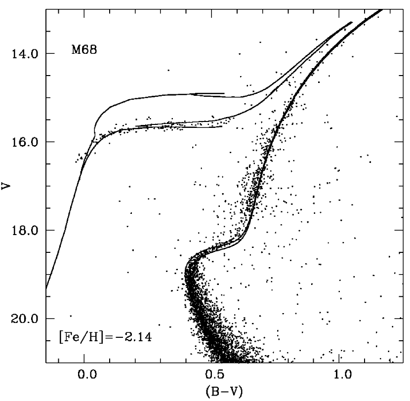
Figure 13: $BV$ diagram of M68 (data from Walker 1994) compared to [Fe/H]=$-$2.14, 11 and 12 Gyr old isochrones. See text for details.

The figures 13 and 14 show the comparison of our isochrones with the CMD of two Galactic GCs, namely $BV$ data for M68 (data from Walker 1994) and $VI$ data for NGC 362 (data from Bellazzini et al. 2001). A detailed analysis of the fitting to globular cluster CMDs and the study of their age distribution is outside the scope of the paper. As mentioned before, here we wish only to show the level of agreement between our set of models and selected CMDs of Galactic GCs of different [Fe/H] values.

For M68 we display in Fig. 13 our 11 and 12 Gyr old isochrones with [Fe/H]=$-$2.14, corrected for a reddening $E(B-V)=$0.07 and distance modulus $(m-M)_{V}$=15.25. The chosen metallicity is somewhat intermediate among the values [Fe/H]=$-1.99$ on the Carretta & Gratton (1997 – CG97) scale, [Fe/H]=$-2.09$ on the Zinn & West (1984 – ZW84) scale and [Fe/H]=$-$2.40 on the Kraft & Ivans (2003 – KI03) scale. The adopted reddening (necessary to match the location of the observed MS) is in good agreement with the value $E(B-V)=$0.07$\pm$0.01 estimated by Walker (1994). The distance is obtained from the fitting of the theoretical ZAHB to the observed counterpart, and agrees with the value we determined in the HST system (Recio-Blanco et al. 2004). Together with the predicted ZAHB we also display the HB and AGB portion of the 12 Gyr isochrone, for values of the mass loss parameter $\eta$=0.2 and 0.4, respectively.

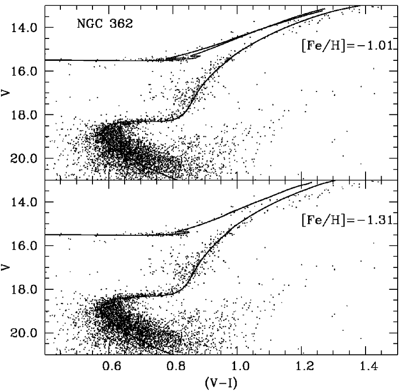
Figure 14: $VI$ diagram of NGC 362 (data from Bellazzini et al. 2001) compared to isochrones with, respectively, [Fe/H]=$-$1.31, t=10 Gyr and [Fe/H]=$-$1.01, t=9 Gyr. See text for details.

Figure 14 displays the comparison with NGC362. NGC 362 has a metallicity [Fe/H]=$-$1.27 on both ZW84 and KI03 scales, and [Fe/H]=$-$1.15 on the CG97 scale; we compare the observed CMD to our isochrones with [Fe/H]=$-$1.31 (t=10 Gyr $E(B-V)=$0.02) and an isochrone with [Fe/H]=$-$1.01 (t=9 Gyr, $E(B-V)=$0.0). Together with the full theoretical ZAHB we display the HB and AGB portion of the isochrones computed with $\eta=0.2$ for [Fe/H]=$-$1.31, and both $\eta$=0.2 and 0.4 for [Fe/H]=$-$1.01. The distance moduli adopted from the fitting of the observed ZAHB are $(m-M)_{V}=14.94$ for [Fe/H]=$-$1.31 and $(m-M)_{V}$=14.86 for [Fe/H]=$-$1.01, consistent with Recio-Blanco et al. (2004 – obtained from our models transformed into the HST flight system) and very close to the MS-fitting distance by Carretta et al. (2000 – $(m-M)_{V}=14.98\pm 0.05$).

We have also performed some comparisons with near infrared data of Galactic globular clusters. Figure 15 shows our 13 Gyr old isochrone with [Fe/H]=$-$2.14, including the full ZAHB plus the HB and AGB evolution computed with $\eta$=0.2, together with a $VJ$ CMD of M92 (Del Principe et al. 2005). We recall that M92 has [Fe/H]=$-$2.16 on the CG97 scale and [Fe/H]=$-$2.24 on the ZW84 scale. We have shifted the models to account for the well established reddening $E(B-V)=$0.02 (Schlegel et al. 1998) and a distance modulus $(m-M)_{J}=14.75$, that corresponds to $(m-M)_{0}=14.72$. This value is within $\sim 1\sigma$ of the empirical MS-fitting distance obtained by Carretta et al. (2000), e.g., $(m-M)_{0}=14.64\pm 0.07$. The dispersion of the observational CMD does not allow us to firmly constrain the derived distance and age; nevertheless the displayed isochrone properly fits the various branches of the observed diagram.

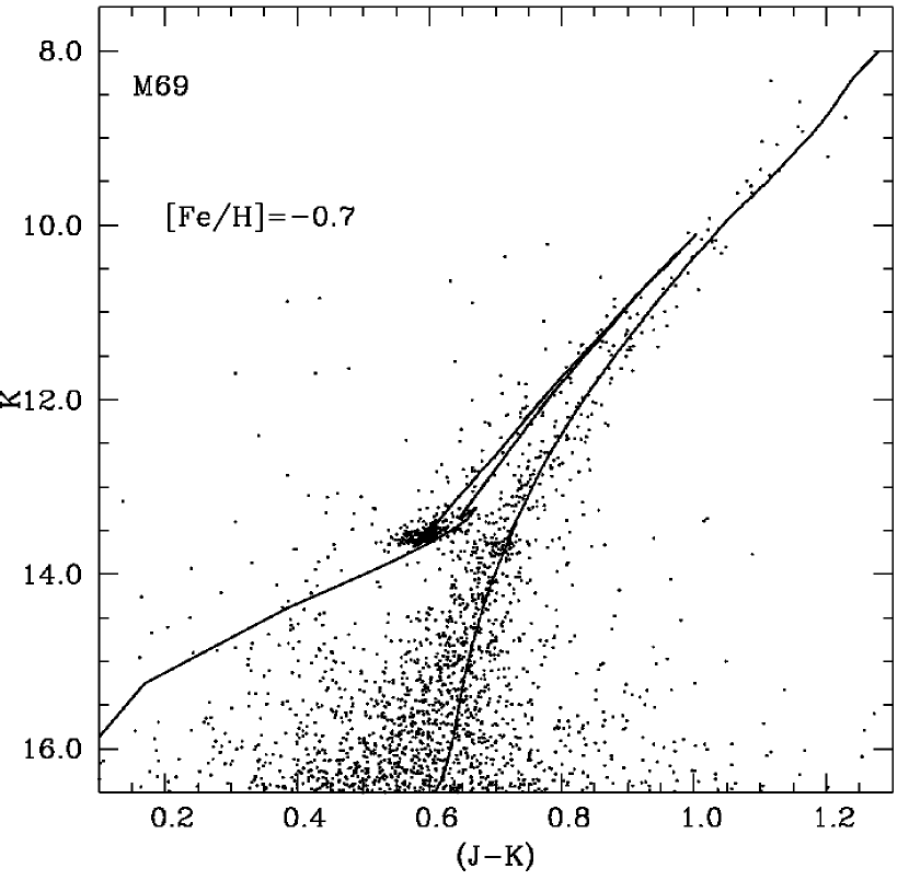
Figure 16: $JK$ diagram of M69 (Valenti et al. 2005) compared to a [Fe/H]=$-$0.7, t=10 Gyr isochrone. See text for details.

A $JK$ CMD of the HB and bright RGB of the [Fe/H]$\sim-0.7$ cluster M69 (Valenti, Origlia & Ferraro 2005) is shown in Figure 16, compared to our 10 Gyr, [Fe/H]=$-0.7$ isochrone (including ZAHB plus the HB and AGB evolution for both $\eta$=0.2 and 0.4). The observational data were on the 2MASS system and have been transformed to the $JK$ system consistent with our color transformations using the empirical relationships by Carpenter (2001). We have adopted a distance modulus $(m-M)_{0}=14.76$ from fitting the theoretical ZAHB to the observed HB, and a reddening $E(B-V)$=0.15; both values are very close to $(m-M)_{0}=14.78$ and $E(B-V)$=0.16 listed in the Harris (1996) catalog. The displayed isochrone traces very well the position of the RGB up to the brightest detected stars.

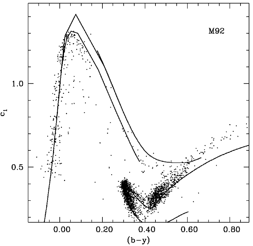
Figure 17: The $[c_{1},b-y]$ diagram of M92 (data from Grundahl et al. 2000), compared to a theoretical isochrone with t=13 Gyr, [Fe/H]=$-$2.14. See text for details.

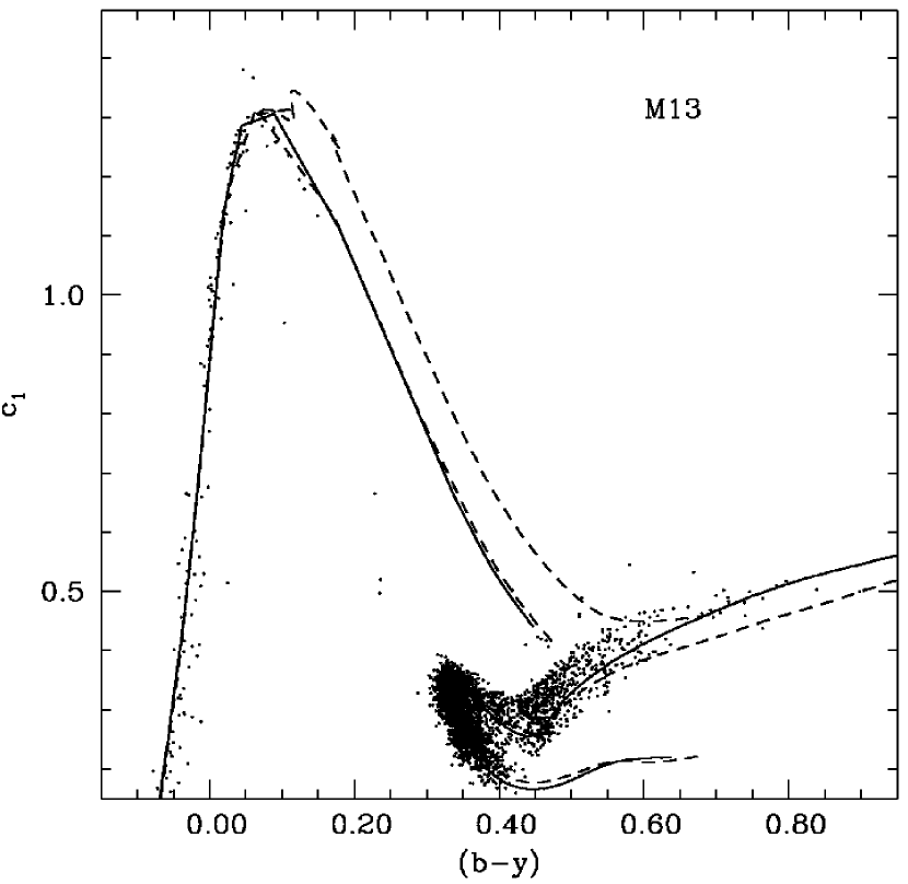
Figure 18: The $[c_{1},b-y]$ diagram of M13 (Grundahl et al. 1998), compared to two theoretical isochrones with, respectively, t=13 Gyr, [Fe/H]=$-$1.62 (solid line), and t=11 Gyr, [Fe/H]=$-$1.31 (dashed line). See text for details.

Figures 17 and 18 show the comparison of our isochrones with the Strömgren $[c_{1},b-y]$ diagrams of M92 and M13 (Grundahl et al. 1998, 2000). In case of M92 we show a 13 Gyr old [Fe/H]=$-$2.14 isochrone computed with $\eta=0.4$, together with the full ZAHB. The only correction applied to the models is for the reddening $E(B-V)$=0.02, where we have used the relationships $E(b-y)=E(B-V)/1.35$, and $c_{1}=c_{0}+0.2E(b-y)$. Notice how the ZAHB sequence runs through the center of the observed HB distribution. This is exactly what one expects from theory, given that the evolution off the ZAHB along the blue part of the HB on this $[c_{1},b-y]$ diagram overlaps with the ZAHB itself. When the ZAHB sequence turns toward the red, theoretical models show a value of $c_{1}$ slightly larger than observed. The isochrones overlap to various degrees all other main branches of the observed diagram, including the RGB. One has also to notice the spread along the observed RGB, due to the large scatter in $c_{1}$ caused by star-to-star differences in the abundance of nitrogen (see, e.g. Grundahl et al. 1998).

In case of M13 (see Fig. 18) we have displayed two isochrones and ZAHBs with, respectively, t=13 Gyr, [Fe/H]=$-$1.62, and t=11 Gyr, [Fe/H]=$-$1.31. This accounts for the uncertainty in M13 iron content, which is [Fe/H]=$-1.39$ according to CG97, [Fe/H]$\sim-$1.5 according to KI03 and [Fe/H]=$-1.65$ according to ZW84. Only for the [Fe/H]=$-$1.62 isochrone we have displayed the full HB evolution obtained using the Reimers parameter $\eta$=0.4 along the RGB. The models have been shifted for a reddening $E(B-V)$=0.03, very close to the value $E(B-V)$=0.02 given by Schlegel et al. (1998). The level of agreement between theory and observations is similar to the case of M92. Notice again the wide RGB, as for M92 (see Fig. 17).

5.2 Integrated photometric properties

We show here a few comparisons of integrated properties extracted from our isochrone sets, e.g. Surface Brightness Fluctuations (SBFs) in $V$ and $I$, plus $(B-V)$ and $(V-I)$ integrated colors of a sample of Galactic GCs. They can be considered as a global test of the accuracy of the bolometric corrections, colors and evolutionary timescales along the relevant phases. We selected GCs whose SBFs in $V$ and $I$ have been determined by Ajhar & Tonry (1994), and whose distances have been estimated by Recio-Blanco et al. (2005) using our $\alpha$-enhanced ZAHB models. As for the integrated colors, we considered the clusters with both $(V-I)$ and $(B-V)$ integrated photometry plus reddenings and [Fe/H] values available in the latest version of the Harris (1996) catalog, which are an average of various sources.

It is important to remark that the $V$ and $I$ SBFs, and the integrated $(B-V)$ and $(V-I)$ colors are very weakly affected by the full thermal pulse phase and by MS masses below 0.5$M_{\odot}$ (presently not included in our database – see, e.g., Brocato et al. 2000, Cantiello et al. 2003).

The theoretical fluctuation magnitudes have been as usual computed from the fluctuation luminosity $\bar{L}$ in the selected photometric band, given by

$$\bar{L}=\frac{\sum n_{i}L_{i}^{2}}{\sum n_{i}L_{i}}$$

where $n_{i}$ is the number of stars of type $i$ and luminosity $L_{i}$. These sums have been performed along the appropriate isochrone, populated according to a Salpeter initial mass function (the integrated colors have also been computed using the same initial mass function).

Figure 19 shows the comparison between the observed GC $\bar{I}$ and $\bar{V}$ fluctuation magnitudes, and the theoretical counterpart obtained from our 10 Gyr $\eta=0.2$ isochrones. In order to show the effect of the uncertain [Fe/H] scale we have considered both the ZW84 and CG97 values. The 1$\sigma$ error bars of the observational points have been obtained by adding in quadrature the 1$\sigma$ errors given by Ajhar & Tonry (1994) and the errors on the individual distance moduli given by Recio-Blanco et al. (2005). The theoretical fluctuation magnitudes trace very well the observations; the effect of a larger age (e.g. 13 instead of 10 Gyr) and a bluer HB ($\eta$=0.4 instead of $\eta$=0.2) are negligible on this plot. As noticed by our referee, two clusters, namely NGC 6652 and NGC 6723 (with [Fe/H]$\sim-$1.0) are systematically discrepant in both the $\bar{V}$ and $\bar{I}$ fluctuation magnitudes, by about 0.2-0.4 mag. It is difficult to point out a precise reason for this discrepancy – which is at the level of at most $\sim 3\sigma$ – although we believe it is possible to exclude an underestimate of the distances to these two clusters by such a large amount. Here we just notice that a similar discrepancy in $\bar{V}$ and $\bar{I}$ can be found in the analysis by Cantiello et al. (2003 – their Fig. 12), who use their own SBF models, [Fe/H] and distances from the Harris (1996) catalog.

A comparison with the observed $(V-I)$ and $(B-V)$ integrated colors is displayed in Fig. 20. The observed colors have been dereddened using the $E(B-V)$ values given in the Harris’ catalog. Given the heterogeneous sources for the observational data one can only discuss the general agreement with theory. Not surprisingly, the integrated $(V-I)$ is very weakly sensitive to age and also to the assumed value of $\eta$, being mainly affected by [Fe/H]. Our models trace very well the observed trend of $(V-I)$ with [Fe/H]. The $(B-V)$ color is more sensitive to both the age and HB morphology; even in this case the models reproduce well the observations.

6 Summary

This paper presents an extension of the scaled-solar stellar model and isochrone database of Paper I, to include an $\alpha$-enhanced ([$\alpha$/Fe]=+0.40) metal distribution.

The models have been computed by using the same sources for the input physics and the same stellar evolution code of Paper I. They are based on the most updated stellar physics available, and are fully consistent with our scaled-solar database. This allows one to disentangle unambiguously the effect of different heavy element distributions when analizing the properties of stellar populations.

The database covers a wide metallicity range suitable for both metal-poor stars, such as extreme Population II objects, and metal-rich stars such as the ones hosted by the Galactic bulge and elliptical galaxies. The adopted initial He content for the most metal-poor stellar models is consistent with recent predictions based on CMB analysis and the R-parameter investigations on a large sample of Galactic GCs, and the adopted He-enrichment ratio accounts for the initial solar He abundance based on our calibration of the Solar Standard Model.

Current database allows the computations of isochrone sets covering a wide range of stellar ages. We are already working to extend our computations to the end of the thermal pulse phase along the AGB.

For each chemical composition in our grid, we computed an extended set of HB models corresponding to an RGB progenitor whose age at the He flash is of the order of $\sim 13$ Gyr, i.e., suitable for investigating the properties of HB stars in old stellar systems. So far, this is the most complete and homogeneous set of HB models for an $\alpha-$enhanced metal distribution, available in literature.

As in Paper I, we devote great care to bolometric corrections and color-$T_{eff}$ transformations. We have been able to use CT based on a metal distribution consistent with that adopted for the evolutionary computations. This opportunity allowed us to extend the investigation performed by Cassisi et al. (2004) to the high metallicity regime and more narrow photometric bands such as the Strömgren filters. Our analysis makes more evident the need to employ appropriate $\alpha$-enhanced CT, especially at high metallicities.

The evolutionary tracks and isochrones are normalized in such a way that they can be easily and directly included in any population synthesis tool by requiring a minimum amount of work.

We have discussed some relevant comparisons between our theoretical framework and empirical data for both unevolved field MS stars with accurate distance and metallicity estimates, and Galactic GCs with accurate photometry in various photometric systems. As a whole we notice an agreement between theory and observations.

The whole library is made available to the scientific community in an easy and direct way through a purpose built WEB site, the same that makes public our scaled-solar database. This WEB site is continuously updated to include additional theoretical models, fully consistent with those presented here and in Paper I. In collaboration with D. Cordier, a big effort is being made to prepare some WEB interactive interfaces that allow users to compute their desired isochrones, evolutionary tracks, luminosity functions and synthetic CMDs.

Table 1: The adopted $\alpha$-enhanced heavy element mixture

element	Number fraction	Mass fraction
C	0.108211	0.076451
N	0.028462	0.023450
O	0.714945	0.672836
Ne	0.071502	0.084869
Na	0.000652	0.000882
Mg	0.029125	0.041639
Al	0.000900	0.001428
Si	0.021591	0.035669
P	0.000086	0.000157
S	0.010575	0.019942
Cl	0.000096	0.000201
Ar	0.001010	0.002373
K	0.000040	0.000092
Ca	0.002210	0.005209
Ti	0.000137	0.000387
Cr	0.000145	0.000443
Mn	0.000075	0.000242
Fe	0.009642	0.031675
Ni	0.000595	0.002056

Table 2: Initial chemical compositions of our model grid.

$Z$	$Y$	[Fe/H]	[M/H]
0.0001	0.245	$-$2.62	$-$2.27
0.0003	0.245	$-$2.14	$-$1.79
0.0006	0.246	$-$1.84	$-$1.49
0.0010	0.246	$-$1.62	$-$1.27
0.0020	0.248	$-$1.31	$-$0.96
0.0040	0.251	$-$1.01	$-$0.66
0.0080	0.256	$-$0.70	$-$0.35
0.0100	0.259	$-$0.60	$-$0.25
0.0198	0.273	$-$0.29	0.06
0.0300	0.288	$-$0.09	0.26
0.0400	0.303	0.05	0.40

Table 3: Selected properties of ZAHB stellar models

$Z$	$[Fe/H]$	$M_{pr}/M_{\odot}$	$He_{sur}$	$M_{cHe}/M_{\odot}$	$M_{3.85}/M_{\odot}$	$log(L_{3.85}/L_{\odot})$	$M_{V,3.85}$
0.0001	$-$2.62	0.80	0.253	0.5028	0.802	1.7573	0.375
0.0003	$-$2.14	0.80	0.255	0.4969	0.710	1.7142	0.479
0.0006	$-$1.84	0.80	0.258	0.4934	0.668	1.6955	0.518
0.0010	$-$1.62	0.80	0.259	0.4905	0.642	1.6764	0.559
0.0020	$-$1.31	0.80	0.262	0.4877	0.613	1.6510	0.615
0.0040	$-$1.01	0.80	0.266	0.4845	0.589	1.6161	0.691
0.0080	$-$0.70	0.90	0.276	0.4795	0.567	1.5705	0.812
0.0100	$-$0.60	0.90	0.279	0.4781	0.561	1.5545	0.825
0.0198	$-$0.29	1.00	0.296	0.4713	0.542	1.5025	0.948
0.0300	$-$0.09	1.00	0.310	0.4656	0.529	1.4753	0.998
0.0400	0.05	1.00	0.324	0.4603	0.519	1.4657	1.015

Figure 3: Comparison between an $\alpha-$enhanced (solid line) and scaled-solar (dashed line) HB tracks in the instability strip, for the labeled values of metallicity and total mass.

Figure 4: CMDs of 12 Gyr old $\alpha-$enhanced isochrones with the labeled metallicities. Three different sets of CT transformations have been employed. Solid lines represent $\alpha-$enhanced transformations with the appropriate metal mixture; long dashed lines denote scaled-solar transformations with the same [Fe/H] of the $\alpha-$enhanced isochrone, whereas short dashed lines display the case of scaled-solar transformations with the same [M/H] of the $\alpha-$enhanced isochrone.

Figure 5: As fig.4, but for Strömgren colors.

Figure 6: $\alpha-$enhanced isochrones with age in the range 10-14 Gyr at step of 1 Gyr, transformed in the $[c_{1},b-y]$ diagram by using $\alpha-$enhanced. The dashed line shows the location of one of these isochrones, namely the 12 Gyr old one, but transformed by using alternatively a scaled-solar CT at the same global metallicity (left panel) or at the same [Fe/H] of the $\alpha-$enhanced one (right panel).

Figure 7: Comparison between our 12 Gyr old isochrone (solid line) with the labeled chemical composition, and a 12 Gyr old, $Z=0.008$ $\alpha$-enhanced isochrone (dashed line) from Salaris & Weiss (1998).

Figure 8: Comparison between our 12 Gyr old isochrone (solid line) with the labeled chemical composition, and a 12 Gyr old, $Z=0.008$ $\alpha$-enhanced isochrone (dashed line) from Salasnich et al (2000). The inset shows an enlargement of the ZAHB region.

Figure 9: As in Fig. 8, but for an age of 500 Myr.

Figure 10: Left panel: comparison between our 12 Gyr old isochrone (solid line) with the labeled chemical composition, and a 12 Gyr old isochrone (dashed line) from Vandenberg et al. (2000) with the same $Z$. Right panel: as the left panel but for $Z=0.01$.

Figure 11: Comparison between our 13 Gyr and 600 Myr old isochrones for the labeled composition, with the $Y$=0.270, $Z$=0.02, [$\alpha$/Fe]=0.3 isochrones of the same ages by Kim et al. (2002).

Figure 12: Comparison of the CMD of a sample of field subdwarfs with Hipparcos parallaxes, metallicity and reddening determinations from Carretta et al. (2000), and our $\alpha$-enhanced isochrones. The full sample is divided into four subsamples (displayed in each panel with filled circles) with the labeled average [Fe/H]. Isochrones from our database with age of 13 Gyr and [Fe/H] equal to $-$1.85, $-$1.62, $-$1.31 and $-$1.01 are displayed.

Figure 15: $VJ$ diagram of M92 (data from Del Principe et al. 2005) compared to an isochrone with [Fe/H]=$-$2.14, t=13 Gyr. See text for details.

Figure 19: $V$ and $I$ fluctuation magnitudes for a sample of Galactic GCs (Ajhar & Tonry 1994) compared to the theoretical predictions. See text for details.

Figure 20: Integrated colors of Galactic GCs from Harris (1996) compared to the theoretical predictions. See text for details.

References

- (1) Ajhar, E.A., & Tonry, J.L. 1994, ApJ, 429, 557
- (2) Alexander, D. R., & Ferguson, J. W. 1994, ApJ, 437, 879
- (3) Bedin, L.R., Cassisi, S., Castelli, F., Piotto, G., Anderson, J., Salaris, M., Momany, Y., & Pietrinferni, A., 2005, MNRAS, 357, 1038
- (4) Bellazzini, M., Fusi Pecci, F., Ferraro, F.R., Galleti, S., Catelan, M., & Landsman, W.B. 2001, AJ 122, 2569
- (5) Bencivenni, D., Castellani, V., Tornambé, A., & Weiss, A. 1989, ApJS, 71, 109
- (6) Bergbusch, P.A., & VandenBerg, D.A. 1992, ApJS, 81, 163
- (7) Böhm-Vitense, E. 1958, Z. Astrophys., 46, 108
- (8) Brocato, E., Castellani, V., Poli, F.M., & Raimondo, G.2000, A&AS, 146, 91
- (9) Cantiello, M., Raimondo, G., Brocato, E., & Capaccioli, M. 2003, AJ, 125, 2783
- (10) Caputo, F., Castellani, V., Chieffi, A., Pulone, L., & Tornambé, A. 1989, ApJ, 340, 241
- (11) Carney, B.W. 1996, PASP, 108, 900
- (12) Carpenter, J. M. 2001, AJ, 121, 2851
- (13) Carretta, E., & Gratton, R.G. 1997, A&AS, 121, 95
- (14) Carretta, E., Gratton, R.G. Clementini, G., Fusi Pecci, F. 2000, ApJ, 533, 215
- (15) Cassisi, S., Salaris, M., Castelli, F., & Pietrinferni, A. 2004, ApJ, 616, 498
- (16) Castelli, F., & Kurucz, R.L. 2003, IAU Symposium 210, eds. N. Piskunov, W.W. Weiss, and D.F. Gray, p.A20 (astro-ph/0405087)
- (17) Chaboyer, B., Sarajedini, A., & Demarque, P. 1992, ApJ, 394, 515
- (18) Cox, J.P., & Giuli, R.T. 1968, Principles of stellar structure (London: Gordon & Breach)
- (19) De Angeli, F., Piotto, G., Cassisi, S., Busso, G., Recio-Blanco, A., Salaris, M., Aparicio, A., & Rosenberg, A. 2005, AJ, 130, 116
- (20) Del Principe, M., Piersimoni, A.M., Bono, G., Di Paola, A., Dolci, M., & Marconi, M. 2005, AJ, 129, 2714
- (21) Dorman, B. 1992, ApJS, 81, 221
- (22) Girardi, L., Bressan, A., Bertelli, G., & Chiosi, C. 2000, A&AS, 141, 371
- (23) Gratton,R., Sneden, C., & Carretta, E. 2004, ARAA, 42, 385
- (24) Grevesse, N., & Noels, A. 1993, in Origin and Evolution of the Elements, ed. N. Prantzos, E. Vangioni-Flam, & M. Cassé (Cambridge: Cambridge Univ. Press), 14
- (25) Grundahl, F., VandenBerg, D.A., & Andersen, M.I. 1998, ApJ, 179, L182
- (26) Grundahl, F., VandenBerg, D.A., Bell, R.A., Andersen, M.I., & Stetson, P.B. 2000, AJ, 120, 1884
- (27) Harris, W.E. 1996, AJ, 112, 1487
- (28) Kim., Y.-C., Demarque, P., Yi, S., & Alexander, D.R. 2002, ApJS, 143, 499
- (29) Kraft, R.P., & Ivans, I.I. 2003, PASP, 115, 143
- (30) Iglesias, C. A., & Rogers, F. J. 1996, ApJ, 464, 943
- (31) Marigo, P., Bressan, A., & Chiosi, C. 1996, A&A, 313, 545
- (32) McWilliam, A., & Rich, M.R. 2004, in Origin and evolution of the elements, A. McWilliam and M. Rauch eds., Carnegie Observatories Astrophysics Series, vol.4, p.38
- (33) Pietrinferni, A., Cassisi, S., Salaris, M., & Castelli, F. 2004, ApJ, 612, 168
- (34) Potekhin, A. Y., Chabrier, G., & Shibanov, Y. A. 1999, PhRvE, 60, 2193
- (35) Recio-Blanco, A. et al. 2005, A&A, 432, 851
- (36) Reimers, D. 1975, Mem. Soc. R. Sci. Liége, 8, 369
- (37) Relyea, L. J., & Kurucz, R. L. 1978, ApJS, 37, 45
- (38) Ryan, S., Norris, J.E., & Bessel, M.S. 1991, AJ, 102, 303
- (39) Salaris, M., Chieffi, A., & Straniero, O. 1993, ApJ, 414, 580
- (40) Salaris, M., Degl’Innocenti, S., & Weiss, A. 1997, ApJ, 484, 986
- (41) Salaris, M., & Weiss, A. 1998, A&A, 335, 943
- (42) Salaris, M., Riello, M., Cassisi, S., & Piotto, G. 2004, A&A, 420, 911
- (43) Salasnich, B., Girardi, L., Weiss, A., & Chiosi, C. 2000, A&A, 361, 1023
- (44) Schlegel, D.J., Finkbeiner, D.P., & Davis, M. 1998, ApJ, 500, 525
- (45) Sneden, C. 2004, Mem.S.A.It., 75, 267
- (46) Spergel, D. N., Verde, L., Peiris, H. V., et al. 2003, ApJS, 148, 175
- (47) Tantalo, R., Chiosi, C., & Bressan, A. 1998, A&A, 333, 419
- (48) Trager, S.C., Faber, S.M., Worthey, G., & Gonzalez, J.J. 2000, AJ, 119, 1645
- (49) Valenti, E., Origlia, L., & Ferraro, F.R. 2005, MNRAS, 361, 272
- (50) VandenBerg, D. A. 2000. ApJS, 129, 315
- (51) VandenBerg, D.A., & Irwin, A.W. 1997, in Advances in Stellar Evolution, Cambridge University Press, p.22
- (52) VandenBerg, D. A., Swenson, F. J., Rogers, F. J., Iglesias, C. A., & Alexander, D. R. 2000, ApJ, 532, 430
- (53) Zinn, R., & West, M.J. 1984, ApJS, 55, 45
- (54) Walker, A.R. 1994, AJ, 108, 555
- (55) Weiss, A., Peletier, R.F., & Matteucci, F. 1995, A&A, 296, 73
- (56) Worthey, G., Faber, S.M., & Gonzalez, J.J. 1992, ApJ, 398, 69
- (57) Yi, S., Demarque, P., Kim, Y.-C., Lee, Y.-W., Ree, C. H., Lejeune, T., & Barnes, S., 2001, ApJ, 136, 417