IMAGING THE DUST TRAIL AND NECKLINE OF 67P/CHURYUMOV-GERASIMENKO

Abstract

We report on the results of nearly 10 hours of integration of the dust trail and neckline of comet 67P/Churyumov-Gerasimenko (67P henceforth) using the Wide Field Imager at the ESO/MPG 2.2m telescope in La Silla. The data was obtained in April 2004 when the comet was at a heliocentric distance of 4.7 AU outbound. 67P is the target of the Rosetta spacecraft of the European Space Agency. Studying the trail and neckline can contribute to the quantification of mm-sized dust grains released by the comet. We describe the data reduction and derive lower limits for the surface brightness. In the processed image, the angular separation of trail and neckline is resolved. We do not detect a coma of small, recently emitted grains.

1 INTRODUCTION

The trajectories of cometary dust particles are – to first order – determined by their emission speed relative to the nucleus and by the ratio $\beta$ of solar radiation pressure to solar gravity. Both quantities decrease with increasing particle size when the latter is large compared to the wavelengths of sunlight.
Large (mm/cm-sized) dust grains remain close to the orbit of their parent comet for many revolutions around the sun, appearing to the observer as a long, line-shaped structure, the comet’s dust trail. The emission of such particles is thought to be the principal mechanism by which a comet loses refractory mass to the interplanetary dust environment sykes-walker1992a . Trails of eight short-period comets were first observed with IRAS in 1983 sykes-lebofsky1986 ; sykes-hunten1986 , one of them being that of 67P.
Of similar shape is the neckline kimura-liu1977 which consists of dust released from the comet at a true anomaly of 180^∘ before observation. In our case this corresponds to emission in mid-July 2002, roughly a month before perihelion passage. An observer close to the comet’s orbital plane will see the neckline as a thin bright line, slightly inclined with respect to the projected orbit. Particles in the neckline are younger and on average smaller than in the trail.
Comet trails and necklines are best studied when separated from smaller dust grains. The latter are released at higher relative speeds and are subject to stronger radiation pressure. They disperse in space on timescales of weeks to months after their emission, and their presence is not expected in the vicinity of an inactive comet far from the sun. In this circumstance lies the appeal of observing a cometary trail or neckline at large heliocentric distance, even despite the then fainter surface brightness.
In Section 2, we describe and discuss the processing of the raw data. This is followed in Section 3 by the interpretation of the obtained image paying special attention to the discrimination between dust trail and neckline. The results are summarised in Section 4.

2 DATA ACQUISITION AND PROCESSING

67P was observed in April 2004 with the Wide Field Imager (WFI) at the ESO/MPG 2.2m telescope in La Silla. The heliocentric and geocentric distances of the comet were 4.7 AU and 3.7 AU, respectively. The total integration time was 9.8 h. 45 minutes were done on 2 April; the remaining time was split equally over the four consecutive nights of 18 – 21 April. We discarded the exposures taken on 18 April, which were highly contaminated by stray light from a star of 4th magnitude outside but close to the instrument field of view (FOV). The remaining data comprises 50 images of 540 s exposure time each. The physical width of one pixel is 15 $\mu$m corresponding to 0.238^′′. In order to maximise sensitivity, 3$\times$3 on-chip pixel binning was used. Each image is a mosaic of 8 CCDs covering a total FOV of 34^′$\times$33^′. No filter was applied.
The data processing was done with IRAF. A thorough discussion of the peculiarities of WFI data and the individual steps of their reduction is given in erben-schirmer2005 . The raw images were bias-subtracted, flatfielded, corrected for airmass, and a mean sky-brightness was subtracted. They were then average-combined while masking stellar objects as described by ishiguro-sarugaku_subm . In order to increase the signal-to-noise ratio (SNR), a spatial averaging filter was applied to the resulting image. An approximate flux calibration was achieved using field stars.
The raw images were characterised by strong fringing, an interference artefact arising in blue-optimised thin-layered CCDs when observing in red wavelengths erben-schirmer2005 . In our data, the fringing pattern was spatially constant, and its amplitude to first order proportional to the background intensity level. Neither twilight nor dome flatfield exposures were used, because the images were taken without filter and the spectral properties of the night sky are different from those of the twilight sky or lamp. Instead, superflats were built from the science data directly. This was possible because due to jittering, stellar objects were in different positions on the CCD in successive exposures. The superflats were obtained by median averaging over several normalised images. Thus bright objects were excluded from the combined image while instrument-specific features remained. An optimally smooth and fringe-free background in the flatfielded images was achieved if using five consecutive exposures per superflat. To make different images comparable a mean sky level was subtracted from each. Airmass correction was done assuming a mean extinction coefficient for La Silla of 0.15 mag/airmass.
In the following, we call the data thus obtained the “corrected single images”. They were subsequently processed in two different manners in order to, first, allow for an approximate flux calibration using field stars and, second, obtain the final image of the trail. For the flux calibration, SNR was increased by averaging over all corrected single images of a given night with such offsets that stars would superpose. In the combined images, aperture photometry of a set of “solar-type” field stars in the FOVs of the images was done. Stars were considered as “solar-type” when their B-R and R-I filter colours in the USNO-B1.0 catalogue were compatible with solar values within the accuracy of the catalogue of $0.25$ mag (monet-levine2003, ). Only stars with R-magnitudes fainter than $17.7$ could be used, because brighter ones were saturated in the raw data. As R-magnitude we used the mean of the two values given in the catalogue. For all stars $j$ fulfilling the above criteria, the integral flux $I_{j}$ in the combined image was measured (in arbitrary units). By plotting the catalogue R-magnitude $M_{\rm cat}(j)$ versus $-2.5\log_{10}(I_{j})$ and fitting a linear relation

$$M_{\rm cat}(j)=M_{0}-2.5\log_{10}(I_{j})$$ (1)

to the data points, the calibration offset $M_{0}$ was deduced. This procedure was exercised for all four nights independently. The derived values of $M_{0}$ were consistent within the regression errors. We used their mean for further calculations: $M_{0}=32.34\pm 0.02$. We obtain surface brightness values ranging from $27.0$ to $28.4$ mag/arcsec² (in R) for the trail and an average nucleus magnitude of $21.7\pm 0.1$.
The final trail image was obtained by averaging over all corrected single images with such offsets as to align the comet. Due to the relative motion of comet and background objects, the latter would appear in the combined image as short, dashed lines often considerably brighter than the trail. In order to exclude such objects from being considered by the averaging procedure, object masks were applied. The object mask for a given night was created with the IRAF routine objmasks for the star-wise combined images used already for the aperture photometry. Saturated or otherwise bad pixels and the spaces between CCDs were masked as well.
The resulting combined image has a reasonably smooth background and the trail is easily visible (Fig. 1(a)). However, the low mean SNR of 0.6 per individual pixel precludes a quantitative analysis of this image. SNR can be improved by applying a spatial averaging filter which replaces each pixel by the average of its $m\times n$ neighbours (IRAF routine boxcar). The price to pay is loss of spatial resolution. The size of the averaging window should be smaller than the characteristic dimension of the object. Since the trail is very extended in the direction parallel to its axis while narrow perpendicular to it, we chose a rectangular window much larger in the parallel direction than in the perpendicular one. To properly apply the filter, the image was first rotated aligning the trail to the x-axis (rotation by $26.5^{\circ}$ clockwise). In addition, the nucleus was removed, i.e. replaced by an interpolation over the surrounding pixels. We used a filtering window of 200 pixels (140^′′) parallel and 10 pixels (7^′′) perpendicular to the trail axis, increasing SNR per pixel by a factor of 45. The resulting image is shown in Fig. 1(b).

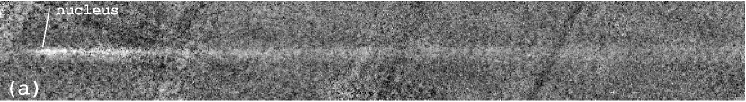
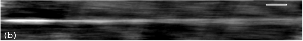
Figure 1: (a) Unfiltered image rotated by 26.5^∘ clockwise. (b) Same image, each pixel being replaced by the average over a neighbourhood of 200 pixels (140^′′) parallel and 10 pixels (7^′′) perpendicular to the trail axis after removal of the nucleus. The filtering window is indicated in the upper right corner. The size of the images is 35^′ x 4.7^′ each. For orientation see Fig. 3. The inclined stripes are remnants of the overscan regions between individual CCDs.

Before embarking upon a quantitative analysis of the data, a certain problem arising from the flatfielding process must be addressed. The difficulty originates from the fact that the surface brightness of the trail was much less than the statistical variation of the background. Moreover, the jittering pattern had not been optimised in direction and amplitude to ensure that trail information could be completely excluded from the superflats.
The superflats were constructed by median averaging over five consecutively taken exposures. In each of these, a given object is found in a different position. Putting it the other way round, if we consider a certain pixel in five consecutive exposures, it will contain a given object at maximum once. This will be discarded by the median filter, and hence the resulting image is free of bright objects. The method fails if the object is less bright than the statistical fluctuation of the background. Since in this case the object-containing pixel will not be significantly brighter than the other four, there is a non-vanishing probability that the median of the five pixels will happen to be the one bearing the object. In the limit of a very faint object, the chances of having it in the median pixel approach 20% which is the probability for one out of five identically distributed pixels to assume the median value. This means that up to 20% of the pixels in the concerned regions of the superflat must be expected to bear trail information. This information is lost from the original image on division by the superflat, and the resulting surface brightness will be 20% too low on average. An accurate estimate of the loss is difficult, and any attempt at a quantitative correction would be highly speculative. It remains always true that the measured brightness is a lower limit.
To nevertheless enable a quantitative comparison with simulated images, we propose to include the details of the flatfielding process into the simulation. The simulated image will then contain (to first order) the same artefacts as the WFI image and should hence be comparable to it.

3 INTERPRETATION

Figure 2: Lower limit brightness profiles along trail and neckline. The scale is linear in intensity but labelled with the corresponding logarithmic R-magnitudes. The profiles are not independent of each other because trail and neckline overlap, especially near the nucleus (see Fig. 1(b)). The apparent shift of the peak to the right of the nucleus is a result of the spatial averaging filter, the brightness dropping more steeply to the left of the nucleus than to its right.

Taking a closer look at the filtered image Fig. 1(b), a splitting of the line-shaped structure can be discerned. The gap between the two parts widens with increasing distance from the nucleus. We have ascertained that the splitting does not result from combining images taken in different nights: It remained if only data acquired in a single night was used, and the predicted position angle of the trail did not change significantly over the period of observation. Hence we presume that the splitting is real.
Using the model described in agarwal-mueller2006_inpress , we find that the expected position angles of trail and neckline are $296.9^{\circ}$ and $296.1^{\circ}$, respectively (measured counterclockwise from north). In Fig. 1, the difference in position angle between the two branches is $0.8^{\circ}\pm 0.2^{\circ}$ which complies well with the anticipated separation of trail and neckline. The same is true for the mean position angle of the feature which is $296.5^{\circ}$. Hence we interpret the upper branch in Fig. 1 as the dust trail and the lower one as the neckline. Trail and neckline are visible up to the edge of the FOV. The length of the orbit section covered is $35^{\prime}$, corresponding to $1.1^{\circ}$ in mean anomaly.
The different ages of dust in the trail and neckline imply that at a given distance from the nucleus trail particles are expected to be larger on average than material in the neckline. If we assume that the size distribution of dust leaving the comet did not change with time (apart from its dependency on the strength of gas drag), the projectional separation of trail and neckline provides us with two manifestations of the same quantity. This puts an additional constraint to any model attempting to reproduce the data.
Fig. 2 shows intensity profiles along the axes of trail and neckline. They are characterised by a pronounced peak around the nucleus and a rather uniform brightness distribution at distances beyond $5^{\prime}$ from the nucleus. According to simulation, the surface brightness in the neckline decreases significantly with growing nucleus distance while it is rather uniform along the trail. Since the influence of radiation pressure decreases with particle size, larger grains remain closer to the nucleus. Therefore, the bright peak in Fig. 2 is likely due to mm/cm-sized particles emitted around perihelion in 2002.

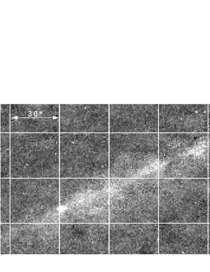
Figure 3: Top: Enlarged view of the nucleus and adjacent region in Fig. 1(a) before rotation. Bottom: A plot of synchrones and syndynes for 19 April 2004. Synchrones are the positions of particles of different $\beta$ emitted at fixed times, labelled in the plot in days before observation. Syndynes show the positions of particles of given $\beta$ (indicated at the right margin) released at varying dates. The negative orbital velocity vector of the comet corresponds to its projected orbit and trail axis. Syndynes of large and synchrones of old particles in the image converge towards this direction. The extended sun-comet vector points to where young, small grains of high $\beta$ are expected to be found. In both images, north is up and east is left.

Fig. 3 shows the near-nucleus region in more detail and a plot of synchrones and syndynes as introduced in finson-probstein1968a for the same observation geometry. Syndynes for small $\beta$ and synchrones for old particles converge towards the direction of the projected comet orbit. In contrast, recently emitted dust of high $\beta$ is expected to be found along the direction of the projected sun-comet vector and to the north-west of it. Given the noisiness of the data, we conclude that we cannot detect sufficient evidence for the presence of small, young particles.

4 Summary

We have observed the dust trail and neckline of comet 67P in April 2004 with the WFI at the ESO/MPG 2.2m telescope when the comet was at a heliocentric distance of 4.7 AU. We do not see a coma of small, recently emitted dust particles around the nucleus. The trail and neckline, however, are visible over the whole section of the comet orbit covered by the image ($1.1^{\circ}$ in mean anomaly). Trail and neckline are separated by slightly different position angles, in agreement with theoretical expectation. We have derived lower limits for the surface brightness of $27.0$ mag/arcsec² close to the nucleus and $28.4$ mag/arcsec² (im R) further out. The enhanced surface brightness around the nucleus is interpreted as the effect of mm/cm-sized dust grains emitted around the perihelion passage in 2002.

5 Acknowledgements

This work is based on observations made with the MPG/ESO 2.2m telescope at the La Silla Observatory under programme ID 072.A-9011(A). It has made use of the USNOFS Image and Catalogue Archive operated by the United States Naval Observatory, Flagstaff Station.

References

- (1) Sykes, M. V. and Walker, R. G. Cometary dust trails. I - Survey. Icarus, 95:180–210, 1992.
- (2) Sykes, M. V., Lebofsky, L. A., Hunten, D. M., and Low, F. The discovery of dust trails in the orbits of periodic comets. Science, 232:1115–1117, 1986.
- (3) Sykes, M. V., Hunten, D. M., and Low, F. J. Preliminary analysis of cometary dust trails. Advances in Space Research, 6:67–78, 1986.
- (4) Kimura, H. and Liu, C. On the structure of cometary dust tails. Chin. Astron., 1:235–264, 1977.
- (5) Erben, T., Schirmer, M., Dietrich, J. P., Cordes, O., Haberzettl, L., Hetterscheidt, M., Hildebrandt, H., Schmithuesen, O., Schneider, P., Simon, P., Deul, E., Hook, R. N., Kaiser, N., Radovich, M., Benoist, C., Nonino, M., Olsen, L. F., Prandoni, I., Wichmann, R., Zaggia, S., Bomans, D., Dettmar, R. J., and Miralles, J. M. GaBoDS: The Garching-Bonn Deep Survey. IV. Methods for the image reduction of multi-chip cameras demonstrated on data from the ESO Wide-Field Imager. Astronomische Nachrichten, 326:432–464, 2005.
- (6) Ishiguro, M. private communication.
- (7) Monet, D. G., Levine, S. E., Canzian, B., Ables, H. D., Bird, A. R., Dahn, C. C., Guetter, H. H., Harris, H. C., Henden, A. A., Leggett, S. K., Levison, H. F., Luginbuhl, C. B., Martini, J., Monet, A. K. B., Munn, J. A., Pier, J. R., Rhodes, A. R., Riepe, B., Sell, S., Stone, R. C., Vrba, F. J., Walker, R. L., Westerhout, G., Brucato, R. J., Reid, I. N., Schoening, W., Hartley, M., Read, M. A., and Tritton, S. B. The USNO-B Catalog. AJ, 125:984–993, 2003.
- (8) Agarwal, J., Müller, M., Böhnhardt, H., and Grün, E. Modelling the large particle environment of comet 67P/Churyumov-Gerasimenko. Advances in Space Research, in press, 2006.
- (9) Finson, M. L. and Probstein, R. F. A theory of dust comets. I. Model and equations. ApJ, 154:327–352, 1968.