Millimeter observation of the SZ effect in the Corona Borealis supercluster

Abstract

We have observed the Corona Borealis supercluster with the Millimeter and Infrared Testa Grigia Observatory (MITO), located in the Italian Alps, at 143, 214, 272, and 353 GHz. We present a description of the measurements, data analysis, and results of the observations together with a comparison with observations performed at 33 GHz with the Very Small Array (VSA) interferometer situated at the Teide Observatory (Tenerife, Spain). Observations have been made in the direction of the supercluster towards a cosmic microwave background (CMB) cold spot previously detected in a VSA temperature map. Observational strategy and data analysis are described in detail, explaining the procedures used to disentangle primary and secondary anisotropies in the resulting maps. From a first level of data analysis we find evidence in MITO data of primary anisotropy but still with room for the presence of secondary anisotropy, especially when VSA results are included. With a second level of data analysis using map making and the maximum entropy method we claim a weak detection of a faint signal compatible with a SZ effect characterized at most by a Comptonization parameter $y=(7.8^{+5.3}_{-4.4})\times 10^{-6}$ 68% CL. The low level of confidence in the presence of a SZ signal invite us to study this sky region with higher sensitivity and angular resolution experiments such as the already-planned upgraded versions of VSA and MITO.

1 Introduction

The cosmic microwave background radiation (CMB) is one of the most powerful tools in cosmology. Distortions of the CMB frequency spectrum due to relic photon inverse Compton scattering with hot electron gas in clusters of galaxies is called the Sunyaev-Zel’dovich effect (SZE) Sunyaev and Zel’dovich (1972); reviews of the effect can be found in Rephaeli (1995), Birkinshaw (1999), and Carlstrom et al.,  (2002). This secondary anisotropy effect produces a brightness change in the CMB that can be detected both at radio frequencies and at millimeter and sub-millimeter wavelengths, appearing as a negative signal (with respect to the average CMB temperature) at frequencies lower than $\sim$217 GHz and as a positive signal at higher frequencies. Its relatively simple spectral behavior and the fact that in the Cosmological Standard Model it is redshift independent, make the SZE a powerful tool, both for investigating the physical properties of the cluster of galaxies through which it is observed and for extracting important cosmological information like the Hubble constant or the absolute temperature of the CMB at the redshift of the cluster of galaxies.

The SZE intensity change depends on the electron density of the scattering medium $n_{e}$ and on the electron temperature $T_{e}$ both integrated over the line of sight (l.o.s. ) $l$, and can be described by the Comptonization parameter $y$:

$$y=\int n_{e}\sigma_{T}\frac{k_{B}T_{e}}{m_{e}c^{2}}dl,$$ (1)

where $\sigma_{T}$ is the Thomson cross section, $k_{B}$ is the Boltzman constant, $m_{e}$ is the electron mass, and $c$ is the light speed in vacuum. In a non-relativistic approximation, the thermal SZE spectral behavior is described, in terms of the thermodynamic temperature change $\Delta T_{SZ}$ with respect to the average CMB temperature $T_{CMB}$, by the expression:

$$\frac{\Delta T_{SZ}(x)}{T_{CMB}}=y(x\cdot coth(x/2)-4),$$ (2)

where $x$ is the adimensional frequency $x=h\nu/(k_{B}T_{CMB})$.

So far, the SZE has only been observed in the direction of clusters of galaxies; however, other objects may also be sources of detectable SZE. Clusters of galaxies are often found in superclusters of galaxies (SCG). The intra-supercluster medium (ISCM) present in their central regions, despite the relatively low density and temperature of the baryon population, may be sufficiently elongated along the l.o.s. to be detectable through SZE even without galaxy clusters being present throughout the same region.

The baryon distribution in the Universe is in fact still an open problem for modern cosmology. The observed baryonic matter in the local Universe obtained from H I absorption, gas and stars in galaxy clusters, and X-ray emission is still small compared to what is predicted by nucleosynthesis (see e.g. Fukugita et al.,  1998), by Ly$\alpha$ forest absorption observations (see e.g. Rauch et al.,  1997), and by measurements of the CMB power spectrum (see e.g. Spergel et al.,  2003). A diffuse baryonic dark matter detection could explain, at least in part, the apparent discrepancy between the observed and the expected baryon density. Simulations of large-scale cosmological hydrodynamic galaxy formation (see e.g. Cen and Ostriker, 1999) show that at low redshift, these missing baryons, which represent approximately half of the total baryon content of the Universe, should lie in the temperature range of $10^{5}\rm K<T<10^{7}\rm K$ in a state of warm-hot gas not yet observed through their EUV and soft-X-ray emission. Yoshida et al. (2005) have studied the temperature structure of this warm-hot intergalactic medium (WHIM).

Hence, superclusters seem to be attractive regions in which to search for these missing baryons. Indeed, many authors have conducted X-ray measurements of their emission (e.g. Persic et al.,  1988, 1990; Day et al.,  1991; Bardelli et al.,  1996; Zappacosta et al.,  2005 Rephaeli and Persic 1992), but finding no compelling evidence for the presence of WHIM in the observed regions. Inside superclusters of galaxies, the outskirts of clusters of galaxies have been studied by Finoguenov (2003), Kaastra et al.,  (2003), and Bonamente et al.,  (2003), who found evidence for soft X-ray excess, which could be due to warm baryonic diffuse matter. These are of fundamental importance in understanding the structure of the superclusters themselves.

In addition to the X-rays, the SZE may represent a useful tool to search for the WHIM because, as stated above, the large path lengths of the CMB photons across SCGs could produce a significant effect. At angular scales of a few square degrees (typical size of the known SCGs), limits on the diffuse SZE have been placed by Banday et al. (1996) and Rubiño-Martín et al. (2000), who cross correlated the COBE DMR all-sky data and the Tenerife data, respectively, with catalogues of clusters of galaxies finding a stringent upper limit of $\approx 8\mu\rm K$ at, respectively, $7^{\circ}$ and $5^{\circ}$ angular scales. However, at smaller angular scales, a deep study of this diffuse emission is only now becoming effective, with the increase in the number of experiments whose primary goal is to map the microwave sky both characterizing primary and secondary CMB anisotropies and extracting important cosmological information from these maps. Statistical work has, for instance, been carried out using WMAP first-year data with given catalogs of galaxy clusters (Hernández-Monteagudo et al.,  2004a, 2004b; Myers et al.,  2004; Lieu et al.,  2005).

In section 2 we briefly report the VSA observation of the Corona Borealis supercluster, and in section 3 the MITO experiment is introduced and the observational strategy is presented. In section 4 we present the use of simulations in the data analysis stage. In sections 5 and 6 data analysis is described with the discussion of the possible sources of contamination. Finally in section 7 we present and discuss the results.

2 VSA observation on the Corona Borealis supercluster

The VSA instrument is a 14 element heterodyne interferometer array with 1.5 GHz bandwidth, tunable between 26 and 36 GHz, situated on the Teide Observatory in Tenerife (see e.g. Watson et al.,  2003). It is the result of an Anglo-Spanish collaboration between the Cavendish Laboratory, the Jodrell Bank Observatory, and the Instituto de Astrofísica de Canarias. In Extended Configuration it uses identical conical corrugated horns 322 mm in diameter with a primary beam of $2^{\circ}.1$ FWHM and a synthesized beam of $\approx 11^{\prime}$ FWHM at 33 GHz.

The Corona Borealis supercluster has been mapped by VSA mainly in the period between the end of 2003 and the middle of 2004 Genova-Santos et al.,  2005a ; 2005b . A major result appearing in these maps is the presence of two strong ($\approx 8\sigma$) temperature decrements near the center of the SCG in directions with no known cluster of galaxies with minimum intensities of -72$\pm$12 and -103$\pm$10 mJy/beam respectively, with typical sizes of $\approx$3 VSA synthesized beams (thermodynamic temperatures correspond respectively to -157$\pm$27 and -230$\pm$23 $\mu$K). The two spots (namely spot B and H in the pointing mosaic carried out by VSA) are centered on: R.A.=$15^{h}25^{m}21^{s}.60$ dec=$+29^{\circ}32^{\prime}40^{\prime\prime}.7$ and R.A.=$15^{h}22^{m}11^{s}.47$ dec=$+28^{\circ}54^{\prime}06^{\prime\prime}.2$ (J2000). Monte Carlo simulations have highlighted the unlikeliness of these spots (especially the strongest one) to be due only to primary CMB anisotropies with a probability 37.82$\%$ and 0.38$\%$ respectively. Press-Schechter and Sheth-Tormen mass functions were used in order to investigate the possibility that these anisotropies could be due to unresolved and unknown cluster of galaxies, showing again a low possibility for this to happen. The probability of these spots arising from SZE, and in particular from extended SZE, is thus what we focus on in this paper.

The evidence of these SCG spots being due to inverse Compton scattering would result from a positive signal at frequencies higher than $\approx$217 GHz, an effect that uniquely characterizes the SZE. Observations have thus been performed at MITO (with four channels centered at 143, 214, 272, and 353 GHz), which is capable of disentangling sources of anisotropy with different spectral behavior.

3 MITO observations

3.1 The instrument

The MITO experiment is a 2.6-m primary mirror telescope equipped with a four channel photometer (FotoMITO) operating from Italian Alps at 3500 m altitude De Petris et al.,   (1999); 2005a . It is a Cassegrain telescope in altitude-azimuthal configuration optimized for differential measurements, thanks to the secondary mirror, which can wobble around the neutral point with digitally controlled wave forms. FotoMITO is a single pixel, multifrequency photometer with four neutron transmutation-doped (NTD) Ge composite bolometers cooled to 290 mK. The 4 K cooled refocusing optics, mesh filters, and beam splitters allow a reduction of the background on the bolometer as well as the selection of the desired frequency bandwidth and throughput, together with the 290 mK cooled Winston cones working as radiation collectors. The working frequencies, summarized in table 1, have been selected to perform efficient SZE studies and to match the 2 mm, 1 mm, and 850 $\mu$m atmospheric windows. The beam of the instrument has a FWHM of $16^{\prime}$ Savini et al.,   (2003) and the pointing accuracy is $\approx 1^{\prime}$ achieved by frequent observation of bright stars close to the source with a CCD camera. The MITO experiment has been efficiently used to perform measurements of the SZE from the Coma Cluster (De Petris et al.,  2002; Savini et al.,  2003) as well as to extract important cosmological information from it Battistelli et al.,   (2002); bat03 (2003). Table 1 gives the main MITO characteristics.

3.2 The observational strategy

Data were collected in 2004 March and include observations on the deepest spot of the VSA map (i.e. spot H), calibration scans on Jupiter, some pointings on Saturn and Tau A used as secondary calibration sources, and routine sky dips to extract information about atmospheric emission.

Sky modulation has been performed by a three fields square-wave-like scanning along constant elevation followed by lock-in demodulation. This allows efficient removal of the atmosphere emission even when it exhibits strong linear gradients parallel to the horizon. The beamthrow was set to $41^{\prime}$ and the modulation frequency to 4.5 Hz with second harmonic demodulation.

Measurements were carried out by performing drift scans (DSs) on the source. This procedure, with respect to antenna nodding (AN) procedure, allows the reduction of bolometer microphonics as the telescope is at rest during the observation. It also helps separation of side-lobe pick-up from sky signal and permits an efficient monitoring of the atmosphere in the ”off-region” position before and after the source crosses the instrument beam; in general, it allows substantial control of many systematics. On the other hand, in scanning mode the effective integration time on the source is reduced, and due to the source motion in the sky, a rotation of the modulation reference plane occurs between various DSs, resulting in a more complicated procedure for scan combination (this problem is also present for AN observations).

We have collected 105 scans across the region of Corona Borealis at the VSA H spot. Each scan is 10 minutes long in R.A.

4 Simulations

Given the adopted scan-mode strategy and the differential measurements, a fitting of the spatial distribution of the observed signals requires information about the instrument (beam aperture and modulation strategy) and about the expected brightness profile of the source. Unfortunately, in the present case, this procedure introduces a higher uncertainty with respect to similar ones already used for SZE observations of galaxy clusters De Petris et al.,   (2002) whose characteristics are well constrained by X-ray observation.

Simulations have thus been performed from the CLEANed VSA Corona Borealis map and compared with real scans. CMB primary anisotropy maps allowing for the presence of secondary anisotropy signal with different shape and intensity have in fact been produced at MITO frequencies convolving the signal with the channels’ response. The maps have then been normalized to the signal we get in the VSA map. Analogue procedures have then been applied to the $13^{\prime}$ FWHM WMAP 90-GHz map with no significant detection mainly due to the low S/N of the first year data in the specific location.

DS procedures have thus been simulated on the computed maps at the experimental coordinates where effective measurements have been carried out. The scan simulation has been performed accounting for the MITO beam size as well as for the bolometer time constants and the lock-in transfer function. Like the real MITO data, simulated scans with the MITO strategy appear as four time ordered data sequences.

The map normalization and the scan simulation procedure automatically account for the effect of beam dilution and reference beam contamination often considered as a later correction included with the form factor. The comparison between the simulations and the real scans accounts for the effect of the MITO window function that would drive a sky measurement away from the real sky temperature because of dilution and field contamination.

Further simulations have been performed on maps calculated from the best-fit analysis in order to determine the most probable maps consistent with MITO data. This method is presented in section 5.5.1.

5 Data analysis

5.1 Preliminary procedures

Our DSs are characterized by offsets due to several sources that create modulated signals difficult to extract from data mainly due to small asymmetries. Offset sources have been studied and simulated and much effort has been spent in order to reduce and stabilize those. However, a small source of offset is present in our data which we can attempt to remove at the data analysis stage through a constant or linear fitting of it. A quadratic fitting did not change the $rms$ value of the residual fluctuation, although it might affect the window function at low multipoles.

Another feature evident in the MITO data is the presence of spikes due to both cosmic rays heating our bolometers and electromagnetic interference. These spikes are simply excluded with a dedicated algorithm.

5.2 Atmospheric transmission

As is well known, even when observing from sites at high altitude, atmospheric transmission at millimeter and submillimeter wavelengths is greatly affected by precipitable water vapor (PWV) content. Measurements of atmospheric emission have thus been taken and compared with models describing atmospheric characteristics in order to perform estimates of its transmission.

Atmospheric emission has been monitored by performing sky dips, i.e. measuring atmospheric emission at different elevations in order to test its dependence on the air mass. Measurements have been performed by focal plane chopping between atmospheric signal and a black body reference (i.e. Eccosorb AN-72) at ambient temperature.

We have used the Atmospheric Transmission at Microwaves (ATM) program Pardo et al.,   (2001) to simulate the atmospheric emission, at different elevations, PWV, atmospheric pressure, and temperature. Uncertainties due to the responsivity determination have been minimized by calculating the ratios between signals at different elevation. Experimental data have then been fitted to the models estimating the value of the PWV for each observing night. In this way we have estimated atmospheric transmission for the four MITO channels during each scan of the observed region. In table 1 we report the average transmissions $<\tau>$ for the four MITO channels.

In order to perform the best atmosphere transmission monitoring simultaneous with the observations, a dedicated spectrometer is under development De Petris et al.,  2005b .

5.3 Calibration

Calibrations are performed observing planet sources such as Jupiter which is one of the brightest ”point-source” at millimeter and sub-millimeter wavelengths. Jupiter has also been used for a precise measurement of the effective beam shape Savini et al.,   (2003). The planet emission at millimeter and sub-millimeter wavelengths has been measured and simulated through many models (we used Moreno, 1998). The lack of information about its emission process results in a typical uncertainty of 10$\%$ on the temperature value. For the four MITO channels we have 171, 171, 170, and 169 K at 143, 213, 272, and 353 GHz, respectively.

From the Jupiter observations, we extract the calibration factors $C$ whose averages are summarized in table 1. DSs have also been performed at different declinations and on different sources such as Saturn and Tau A as a consistency check, to map the sources and to check for bad alignments. The errors are dominated by the 10% uncertainties over the planet absolute temperature. Small differences in $C$ for different nights of observation have been encountered and have been found to be due to the intrinsic drifts in the receiver response and instrumental setups; we have accounted for this by calibrating our signals night by night.

Figure 1 shows the signals detected in the four MITO channels in one of the Jupiter scans.

5.4 Noise filtering and atmospheric decorrelation

As already stated, three field chopping measurements are intrinsically insensitive to offset and linear gradients in the atmospheric emission. However, atmospheric temporal and spatial fluctuations are still present in our data, dominating the cosmological signal of interest. In order to get rid of this contamination, we have applied an atmospheric decorrelation based on the large overlapping of the four MITO channel beams (i.e. deviations are lower than 1$\%$) and the presence of the 353-GHz channel, which is much more sensitive to the atmospheric emission. The basic procedure is to subtract, from the channels at the frequency of cosmological interest, the channel most affected by atmospheric emission, best fitting the factor driving the latter into the other channels. High correlation between the channels is a key ingredient necessary to performing an efficient decorrelation. Uncorrelated signals may be due to different optical depths for different spectral channels, to fluctuations at different altitudes, or to differences in the channel beam (for a detailed discussion on this topic see Melchiorri and Olivo-Melchiorri, 2005).

Analysis and simulations are being carried out in this field and will be described elsewhere (S. De Gregori et al.,  2006, in preparation). The key point is that under average PWV conditions (i.e. $\approx$1mm at Testa Grigia Observatory) and for the MITO spectral bandwidths, the correlation factors between the 353 GHz channel and the others show a high stability against water vapor change for the 143 GHz channel, and with moderate common variation when dealing with the 214 and 272 GHz channels. As a result, the decorrelation operated from the high frequency channel gives good efficiency when applied to the 143 GHz channel while leaving residuals in the other two channels depending on the amount of water vapor change within the duration of the scan. Because of the nonlinear dependence with the PVW of the atmospheric signal in the high frequency channels, these residuals may be characterized by a non-zero average and leave an imprint in our decorrelated signals.

Many scans collected in this observing campaign have shown high enough correlation to allow an efficient subtraction (threshold has been set at 85$\%$); however, in some cases the correlation has not been found high enough to allow the decorrelation procedure to approach the detector noise. In these cases, further filtering procedures have been applied in order to suppress the uncorrelated components in the signals. We have tested different filtering procedures in both real space and Fourier space. These procedures have been found efficient for those scans showing moderately high correlation even if not enough to undergo an efficient decorrelation.

The filtering procedure that we finally implemented is presented in Melchiorri and Olivo-Melchiorri (2005) and consists of passing data through a non linear amplifier that yields an output signal $S_{out}$ related with the input signal $S_{in}$ by

$$S_{out}=S_{in}exp[-\frac{|S_{in}|}{\Gamma}],$$ (3)

with $\Gamma\sim 1\sigma$ to be found from simulations considering the effective uncorrelated noise present in out data. This technique has been applied on the ratios between the various channels. The filter has been calibrated from S/N considerations and has been found efficient in removing non-Gaussian noise components, allowing us to approach the fundamental noise of the detectors. Table 2 shows the $rms$ of the signals of the first three MITO channels before and after the filtering procedure. The systematics introduced by this procedure have been simulated and found to be negligible compared to the random errors we have at the end of the procedure. The non linear amplifier allows us to ”clean” our data of non-Gaussianity in an unbiased way, controlling the systematics.

About 1/3 of the total number of scans have been removed from the analysis for not showing high enough correlation to be efficiently decorrelated. The level of decorrelation has been chosen from simulations. The main average characteristics of our filtered and decorrelated scans are reported in table 2. We have reported the average correlation factors for the first three channels with the 353 GHz channel before and after the filtering procedure, color ratios with respect to the 353-GHz channel together with the dispersion of the other channels, the $rms$ before and after the filtering procedure and the decorrelation.

Once decorrelated, the scans have been found to be Gaussian distributed around their average values. In this case, the impact on the results has also been found to be negligible by applying the process to simulated data sets.

5.5 Best fit

We have applied different methods to extract the information of interest from our cleaned and decorrelated scans. They give consistent results, and meaningful information has finally been extracted by applying maximum entropy method (MEM) to produce the final maps, Monte Carlo (MC) simulations for estimating the errors and maximum likelihood analysis to determine the effective contribution of primary and secondary anisotropies in our maps.

As a first attempt we have applied the method already used for SZE extraction from galaxy cluster observation performed by MITO De Petris et al.,   (2002). In this case, the best fitting of the atmospheric correlation factors is performed together with the best fitting of the parameters describing the intensity of the observed cosmological signal. The latter factors are in fact multiplied by the simulations presented in section 4, which describe the expected shape of the detected signal. For each scan, we have thus performed a maximum likelihood analysis and the results have been combined to extract the final result. Different hypotheses have been tested by using different simulations. This procedure introduces, in the present case, a higher uncertainty with respect to galaxy cluster observations that take advantage of detailed physical information arising from X-ray observations. As a result, the combination of the fits does not allow us to extract meaningful conclusions due to the lack of information about the physical properties of the diffuse gas present in the observed region.

An alternative approach consists of performing the decorrelation without subtracting the simulation from the 353 GHz channel. This procedure introduces a systematic error due to the presence, in the high frequency channel, of a cosmological signal. However, this decorrelation procedure has the advantage of being totally independent of the assumption about the cosmological signal we are searching for. Moreover, due to the large atmospheric signal present in the 353 GHz channel, this systematic error can be kept under control. In table 2 we list the average proportionality factors between the atmospheric noise in the various channels with the 353 GHz channel. The systematics introduced in this way, related to a primary anisotropy detection, contribute factors of around 9%, 7%, and 14% respectively in the first three MITO channels, while for SZE detections they contribute 19%, 129%, and 32% respectively considering the spectral signature of the effect. These corrections are taken into consideration in the subsequent analysis.

The first attempt to use the subsequent scan is by simply averaging them and comparing with the (averaged) simulations performed on the VSA map. It is worth stressing that these averages do not correspond to what is observed in the sky due to the previously mentioned rotation of the reference fields. However, this analysis allows us to extract information on the observed signal from its spectral behavior. From this comparison it is clear that a primary anisotropy signal is present in our data, but still leaving room for further secondary effect like SZE Battistelli et al.,   (2005). However, the combination of our data and simulations do not allow us to $spectrally$ characterize SZE signals present in our data.

5.5.1 Iterative fitting method

We have developed an analysis method capable of generating maps from our differential measurements. Initially this has been performed with an iterative method; starting from the 33 GHz VSA map, we have corrected, at the declination of the central beam of the MITO scans, for the difference between the measured scans and the DS simulation performed on the VSA map. We have then performed simulations on the corrected maps, and we have repeated the procedure until convergence. In this way we obviously introduce a prior based on the assumption that the lateral fields of the MITO scans are those reported in the VSA map. This procedure is based on the hypothesis that the average of the lateral fields in the new MITO corrected maps does not change during the iteration. This is not exactly true, even if this effect has been shown to be small by performing several iterations of the map-making procedure. This procedure is (still) not independent of the VSA observations, but the assumption about the reference MITO fields is weaker than in the method described above. We conclude there is a signal in the H spot that is dominated by a primary anisotropy but with an additional signal with a frequency dependence characteristic of a rising spectrum signal (as the SZ effect is in our spectral range). Still, from simulations we felt that the degeneracy between different realizations of the sky resulting in the same scans patterns is not totally controlled. For this reason we developed further map-making analysis in order to further probe the contributions.

5.5.2 Maximum Entropy method

As map reconstruction is degenerate for differential and interferometer observations, an extra regularizing constraint is required which is conveniently provided by MEM. In order to extract the best representative signal maps from the original data sets, we have carried out the MEM reconstruction for both the MITO decorrelated scans and the gridded VSA visibilities for point H in the Corona Borealis supercluster. We used the same method of fitting modeled data resulting from a trial sky for both data sets in order to be sure of consistency. The sky model used comprises a 70 by 20 pixel image covering R.A. $15^{h}17^{m}-15^{h}27^{m}$ and decl $28^{\circ}30^{\prime}-29^{\circ}18^{\prime}$, in which each pixel brightness represents a free parameter to be found. An iterative gradient method was used to update the sky model and in turn calculate the model scans and visibilities. For each pixel, the gradient was found in order to reduce $\chi^{2}$ together with the constraint of maximizing cross entropy of the sky model. To increase the speed of the iterations the expected response in MITO and VSA data for each trial pixel was pre-calculated and stored in a response matrix. This algorithm was adapted from the version used in Dicker et al.,  (1999) using the positive-negative cross-entropy method of Maisinger et al.,  (1997). After 120 iterations, the solutions had converged and the final sky models were convolved back to a common resolution of $16^{\prime}$. Because of the MITO beam-throw ($41^{\prime}$) and the VSA primary beam (2.^∘0 FWHM), structures on degree scales and larger are attenuated and with the present S/N are impossible to recover. We are therefore limited in what we can say about the broader scale profile of the signal.

A maximum likelihood analysis is then applied pixel by pixel on the extracted maps in order to derive information about the presence of primary and secondary anisotropies in our maps. Results are given in section 7.

The analysis methodology and the codes have been tested using different known signals embedded in both correlated and uncorrelated noise and have yielded a satisfactory level of reproducibility of the results up to a level of random noise of 15$\%$ compared to the actual atmospheric noise (this set the minimum decorrelation threshold of 85$\%$ between our channels). Different tests have been carried out by changing the relative parameter describing the signals as well as the quantities driving the fits and the decorrelations, in order to optimize the latter for a more efficient signal extraction.

6 Contaminants

Signal contamination due to galactic dust has been assessed through the same simulation procedure described in section 4. The dust temperature distribution in the Corona Borealis region has been extracted from the DIRBE-recalibrated IRAS 100 $\mu$m maps presented in Schlegel et al. (1998), and extrapolated to the MITO frequencies and bandwidths through the procedure described by Finkbeiner et al. (1999), assuming their best-fit model for the spectrum of emission. The observed region is quite contaminated at high frequencies and presents structures at the resolution of our interest: the flux estimates for the MITO bands and beam size lead to thermodynamic temperatures of 8.2, 29, 62, and 208 $\mu$K at the nominal coordinates of the H spot. Because of the adopted modulation strategy and the smoothness of the dust distribution or the fact that the mentioned structures are present over a diffuse signal, the signals detected while drift scanning over the region are only sensitive to the far smaller gradients at the angular scales of the MITO chopping amplitude. Therefore, after simulating this observing strategy over the extrapolated maps, the corresponding signals in the observed direction turn out to be 0.2, 0.6, 1.3, and 4.2 $\mu$K at most with a few percent variations due to sky rotation with respect to the modulation axis. Even if small and substantially negligible at the lowest frequencies, this contribution has been accounted for and subtracted from the signal of each scan in the data-set before performing the combined SZE-CMB extraction procedures described above.

In order to quantify the possible contamination from point sources, we have identified all radio sources in the region of observation in the NVSS–1.4 GHz Condon et al.,   (1998) and GB6–4.85 GHz Gregory et al.,   (1996) catalogs. From their fluxes we derived the spectral indexes that were used to extrapolate the fluxes to the four MITO frequencies. All the identified radio sources have predicted fluxes, in each of the four channels, which have no imprint in our data. However, note that we are limited by the sensitivity of the GB6 data, and there could be some undetected sources with rising spectral index and a high flux density at the MITO frequencies. To account for this, we have obtained upper limits for the fluxes at the MITO frequencies of all the identified sources in the NVSS catalog, by assigning a maximum value of the rising spectral index of $\alpha=0.5$ ($S\propto\nu^{\alpha}$). With this method we have found negligible contamination to our observations too.

As we have described, constant and linear atmosphere emission has been subtracted by the differential measurements and correlated temporal and spatial fluctuations have been reduced by the decorrelation procedure. Uncorrelated atmospheric noise is still present in our data and will add to the detector noise. However, MEM has been found to be efficient in extracting sky information from uncorrelated noise. As anticipated in section 5.4, a source of residual atmospheric noise may be present in our data, depending on the variation of PWV within the observational time. This source of contamination is larger at higher frequencies and is present as a common signal in the 214 and 272 GHz channels as a residual of the imperfect decorrelation and of the variation of the PWV content in the drift-scanning procedure.

7 Results and discussion

The results of the analysis described in section 5 are presented in this section. The maximum likelihood analysis on the maps extracted from the MEM has been performed in two steps; by extracting first common signals and then frequency-dependent signals from the different observational channels. We notice that the signals registered by the VSA and the 143 GHz MITO channel are consistent within each other; in the same way, the 214 GHz and 272 GHz channels are consistent within each other. However, when comparing the four channels at once to perform the extraction of the CMB components characterizing our signals (primary anisotropy and SZE), a third component is evident in the two high-frequency channels, which does not allow the extraction of meaningful information. A possible origin for the further component could be in dust residuals, which have been carefully checked, or in atmospheric residuals present in the 214 and 272 GHz channels due to variable PWV, as suggested in section 6.

In order to perform a meaningful analysis, we have therefore calculated the signal separation at low frequency (i.e. 33 and 143 GHz) and again at high frequency (i.e. 214 and 272 GHz), and we use the low-frequency determination of the primary anisotropy to infer the third additional component. As a result, we find evidence of a small signal common to all the four channels with a spectral behavior typical of the SZE. This signal is restricted to an area of approximately $15^{\prime}$ in both right ascension and declination, with an apparent shift towards lower right ascension with respect to the primary anisotropy spot although the low S/N does not allow us to fully describe the shape of the emitting region; the maximum signal corresponds to the pixel at coordinates $R.A.\rm(J2000)=15^{h}21^{m}42^{s}$ and $\delta\rm(J2000)=28^{\circ}50^{\prime}24^{\prime\prime}$ (in the $6^{\prime}$ resolution binned maps) with a maximum intensity of the Comptonization parameter of $y=(7.8^{+5.3}_{-4.4})\times 10^{-6}$ 68% CL. The signal observed by VSA is dominated by a primary anisotropy with a small contribution from SZE. In a more conservative attitude, with 95% CL uncertainties, our observations could put an upper limit of y$<1.8$ $10^{-5}$ to diffuse/unknown-cluster SZ emission in the studied region.

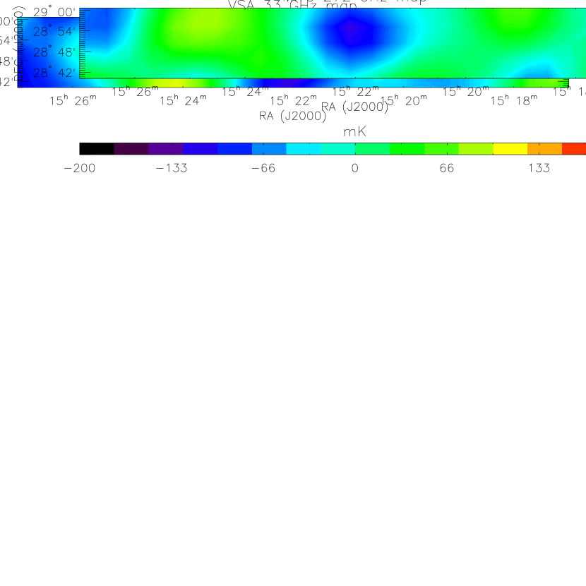
Figure 2: Strip of thermodynamic temperature maps derived from the MEM for VSA and the three MITO channels.

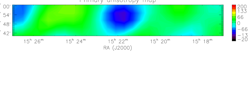
Figure 3: Primary anisotropy and SZE maps derived by maximum likelihood. A spotis evident in the SZ map. This seems to be not resolved by the MITO beam even though the low S/N does not allow a complete description of it.

In figure 2 we show the maps of the observed sky region derived from MEM for VSA and the 3 MITO channels (excluding the 353-GHz channel used for atmospheric subtraction) in terms of thermodynamic temperatures. In the high-frequency channels we have subtracted the third component found at those frequencies so that only the CMB (primary and secondary effects) is present. In figure 3, the maximum-likelihood-derived maps for the primary anisotropy and for the SZ effect (Rayleigh-Jeans thermodynamic temperatures) are given.

In figure 4 we present a cut at $\delta=28^{\circ}50^{\prime}24^{\prime\prime}$ of the derived anisotropy maps extracted for primary and secondary contribution. A minimum is evident in the lower plot corresponding to a RJ thermodynamic temperature of $\Delta T_{SZ}=(-42^{+24}_{-29})\mu$K (RJ), with a primary anisotropy value of $\Delta T_{ani}=(-128^{+21}_{-18})\mu$K, corresponding to the thermodynamic temperatures reported in figure 5. The primary anisotropy signal has been studied using the Monte Carlo simulations method presented in Genova-Santos et al. (2005a): the probability of finding such a spot in a CMB map is now increased to 43$\%$. From the reported values, the fraction of the signal due to SZE is (in the RJ regime) $f\equiv\Delta T_{SZ}/(\Delta T_{SZ}+\Delta T_{ani})=0.25^{+0.21}_{-0.18}$. Note that these values correspond to the maximum entropy sky reconstruction at the resolution of the MITO experiment (i.e. $16^{\prime}$). In order to compare with the VSA measurement at 33 GHz of $-230\pm 23\mu$K, we proceed as follows. Using the same MEM code, we performed two different reconstructions using only the VSA data: one at the MITO resolution ($16^{\prime}$) and another one at the VSA resolution ($11^{\prime}$). In these maps, the H spot is observed with a peak temperature of $-174$ and $-238\mu$K, respectively. These numbers are fully consistent with the inferred signal amplitude using MEM with MITO+VSA at the MITO resolution, being also compatible with the observed amplitude of the decrement in the VSA mosaiced map ($11^{\prime}$ resolution) presented in Genova-Santos et al. (2005a). These results further support the robustness of MEM reconstruction.

We can now use the observed SZ signal to place constraints on the physical parameters describing the gas. As in Genova-Santos et al. (2005a), we shall consider two possibilities for the spatial distribution of the gas.

First, given the angular extension of the feature in the y-parameter map (it is not resolved by the $16^{\prime}$ MITO beam), we can explore the possibility of a cluster of galaxies as responsible for the emission. We shall first estimate the amplitude of the SZ signal at the VSA resolution. If we assume a point-like object, then at $11^{\prime}$ we would expect around $-89\mu$K (RJ temperature). This value is of the same order as the expected SZ signal from the known cluster members of Corona Borealis (see table 1 in Genova-Santos et al.,  2005a). However, it is unlikely that a cluster of galaxies at the redshift of Corona Borealis would have been missed by previous optical surveys. Nevertheless, the possibility of a cluster located at larger distance that was spuriously aligned with the Corona Borealis supercluster cannot be discarded.

On the other hand, we can also consider the case of WHIM being distributed in a filament, aligned along the line of sight of the supercluster with a physical dimension of some 40 Mpc. Using the amplitude of the measured SZ component, we can set the constraints presented in figure 6 in the electron density-temperature plane for such a filament. The shaded regions represent the parameter space constrained from both the SZ observations and the information extracted from the upper limit to the X-ray emission (there is no evidence of emission in the R6 band of the ROSAT XRT/PSPC All-Sky Survey, see Genova-Santos et al.,  2005a). In figure 6 we also consider the +1 $\sigma$ and -1 $\sigma$ cases for the fraction of the signal due to SZ. If we assume for the gas temperature the typical values predicted for the WHIM (0.5-0.8 keV), then we would expect baryon overdensities greater than 400-600 times the mean baryon density in the local Universe, implying a baryonic mass content ($\approx 3\times 10^{14}M_{\odot}$) comparable to the total baryonic mass of the cluster members of the supercluster.

8 Conclusions

We have presented the MITO observation of the Corona Borealis supercluster. The analysis has been performed combining MITO results with VSA observations of the same sky region. A MEM analysis has allowed us to extract maps from our differential measurements. From an analysis of these maps we find evidence of the presence of a strong primary anisotropy signal with a faint secondary SZE signal present in all four channels of the order of $-40\mu$K (RJ). The detection is faint and it seems to be unresolved by the MITO beam. Our results discard a non-Gaussian origin for the CMB spot originally detected by VSA and favor the presence of hot-warm gas in the intracluster region of Corona Borealis with a baryonic mass content of $\approx 3\times 10^{14}M_{\odot}$, even if the hypothesis of an unknown unresolved cluster of galaxies cannot be discarded. Higher sensitivity and angular resolution observations, goals being already pursued both by superextended VSA (Taylor, 2003) and MAD Lamagna et al.,   (2002), will be able to shed a definitive light on the origin of the signal present in this region.

Figure 1: Signal detected observing Jupiter in the four MITO channels.

Figure 4: Primary and secondary SZE anisotropies obtained from VSA and MITO observations at declination $\delta=28^{\circ}50^{\prime}24^{\prime\prime}$ with 1 $\sigma$errors. We have plotted the thermodynamic temperature of the primary anisotropy and the quantity $\Delta T=-2~{}y~{}T_{CMB}$ related to the SZE temperature in the RJ part of the spectrum. There is also a clear minimum corresponding to a maximum value of $y=(7.8^{+5.3}_{-4.4})\times 10^{-6}$ at $R.A.=15^{h}21^{m}42^{s}$.

Figure 5: VSA and MITO detections plotted with the spectral dependence of the resulting superposition of primary and secondary anisotropy (solid line). Both the derivations have been given with 1 $\sigma$ error (dashed line). This figure refers to the maximum SZE signal observed in figure 5 at $R.A.=15^{h}21^{m}42^{s}$ and $\delta=28^{\circ}50^{\prime}24^{\prime\prime}$.

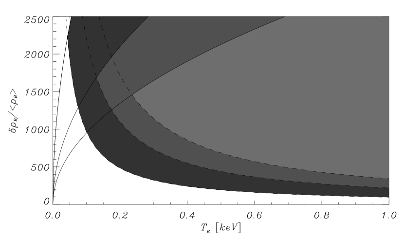
Figure 6: Constraints placed in the over-density (with respect to the mean baryon density) and electron temperature space if we set the SZ component to the nominal value inferred from the analysis in this paper. The filled regions include the allowed parameters combining the ROSAT R6 band observations (represented by the solid line) and an SZE like that detected, obtained assuming a maximum line of sight of 40 Mpc. Lighter and darker colors correspond to -1 $\sigma$ and +1 $\sigma$ respectively.

Table 1: Main MITO characteristics from the March 2004 Campaign. Central frequencies $\nu$, bandwidths (BW), throughput (A$\Omega$), noise-equivalent temperature (NET), average calibration factors (C), and atmospheric transmissions ($\tau$) are included.

Channel	$\nu$(GHz)	$BW$(GHz)	$A\Omega$(cm2sr)	$NET$(mK$\sqrt{s}$)	$<C>(\mu K/nV)$	$<\tau>(\%)$
1	143	15	0.40$\pm$0.02	2.41$\pm$0.24	480$\pm$48	88
2	214	15	0.36$\pm$0.02	2.64$\pm$0.26	376$\pm$38	83
3	272	16	0.34$\pm$0.02	1.40$\pm$0.14	279$\pm$28	81
4	353	13	0.34$\pm$0.02	1.95$\pm$0.19	102$\pm$10	53

Table 2: Average Characteristics of the Decorrelated scans. We have included: the average correlation factors for the first 3 MITO channels with the 353 GHz channel before and after the filtering procedure, the coefficient of proportionality of the atmospheric fluctuations between the various channels and the 353 GHz channel together with the dispersion of these channels, the $rms$ before and after the filtering procedure and the decorrelation.

Parameter	Ch.1	Ch.2	Ch.3
Correlation prefiltering (%)	74	73	81
Correlation postfiltering (%)	95	95	96
Atmospheric factors	10.7	13.4	6.8
Dispersion Atm. factors	1.8	1.6	1.4
$rms$ prefiltering (nV)	9.7	7.7	15.3
$rms$ predecorrelation (nV)	6.2	5.3	11.5
$rms$ postdecorrelation (nV)	2.4	2.1	3.2

References

- Banday et al., (1996) Banday, A.J., et al., 1996, ApJ 468 L85
- Bardelli et al., (1996) Bardelli, S., et al., 1996, A&A 305 435
- Battistelli et al., (2002) Battistelli, E.S., et al., 2002, ApJ 580 L101
- (4) Battistelli, E.S., et al., 2003, ApJ 598 L75
- Battistelli et al., (2005) Battistelli, E.,S., et al., 2005, Proc. of the international school of physics ”Enrico Fermi” 6-16 July 2004 IOS press Melchiorri and Rephaeli eds 379-387
- Bonamente (2003) Bonamente, M., et al., 2003, ApJ 585 722
- Birkinshaw (1999) Birkinshaw 1999, Physiscs Reports 310 97
- Carlstrom et al., (2002) Carlstrom, J.R., Holder, G.P., and Reese, E.D. 2002, ARAA 40 643
- Cen and Ostriker (1999) Cen, R., and Ostriker, J.P. 1999, ApJ 514 1
- Condon et al., (1998) Condon, J. J., et al., 1998, AJ 115 1693
- Day et al., (1991) Day, C.S.R., et al., 1991, MNRAS 252 394
- De Gregori et al., (2006) De Gregori, S., et al., 2006 in preparation
- De Petris et al., (1999) De Petris, M., et al., 1999, New Astronomy 43 297
- De Petris et al., (2002) De Petris, M., et al., 2002, ApJ 574 L119
- (15) De Petris, M., et al., 2005a, Proc. of the international school of physics ”Enrico Fermi” 6-16 July 2004 IOS press Melchiorri and Rephaeli eds 345-354
- (16) De Petris, M., et al., 2005b, EAS Publications Series 14 233-238
- Dicker et al., (1999) Dicker, S.R., et al., 1999, MNRAS 309 750
- Kaastra et al., (2003) Kaastra, S.R., et al., 2003, A&A 397 445
- Finoguenov et al., (2003) Finoguenov, A., 2003, A&A 410 777
- Finkbeiner et al., (1999) Finkbeiner, D.P., Davis, M., and Schlegel, D.J. 1999, ApJ 524 867
- Fukugita et al., (1998) Fukucita, M., Hogan, C.J., and Peebles, P.J. 1998, ApJ 503 518
- (22) Genova-Santos, R., et al., 2005a, MNRAS 363 79
- (23) Genova-Santos, R., et al., 2005b, Proc. of the international school of physics ”Enrico Fermi” 6-16 July 2004 IOS press Melchiorri and Rephaeli eds 389-394
- Gregory et al., (1996) Gregory, P.C., et al., 1996, ApJS 103 427
- (25) Hernández-Monteagudo, C., and Rubiño-Martín, J.A. 2004a, MNRAS 347 430
- (26) Hernández-Monteagudo, C., Genova-Santos, R., and Atrio-Barandela, F. 2004b, ApJ613 2 L89-L92
- Lamagna et al., (2002) Lamagna, L., et al., 2002, AIP Conference Proc., 616, 92, M. De Petris and M. Gervasi eds.
- Lieu et al., (2005) Lieu, F. 2005, ApJ submitted astro-ph/0510160
- Maisinger et al., (1997) Maisinger, K., Hobson, M.P., Lasenby, A.N., 1997, MNRAS 290 313
- Melchiorri and Olivo Melchiorri (2005) Melchiorri, F., and Olivo-Melchiorri, B. 2005, Proc. of the international school of physics ”Enrico Fermi” 6-16 July 2004 IOS press Melchiorri and Rephaeli eds 211-223
- Moreno (1998) Moreno, R. 1998, PhD thesis, University of Paris VI
- Myers et al., (2004) Myers, A.D., et al., 2004, MNRAS 347 L67
- Pardo et al., (2001) Pardo, J.R., et al., 2001, IEEE 49/12 1683-1694
- Persic et al., (1988) Persic, M., Rephaeli, Y., and Boldt, E. 1988, ApJ 327 L1
- (35) Persic, M., et al., 1990, ApJ 364 1
- Rauch et al., (1997) Rauch, M. et al., 1997, ApJ 489 7
- Reaphaeli and Persic (1992) Reaphaeli, Y., and Persic, M. 1992, MNRAS 259 613
- Rephaeli (1995) Rephaeli, Y. 1995, Ann. Rev. Astron. and Ap. 33 541
- Rubiño Martín et al., (2003) Rubiño-Martín, J.A., et al., 2003, MNRAS 341,4 1084
- Rubiño-Martín et al., (2000) Rubiño-Martín, J.A., Atrio-Barandela, F., and Hernández-Monteagudo, C. 2000, ApJ 538, 53
- Savini et al., (2003) Savini, G., et al., 2003, New Astronomy 8-7 727
- Schlegel et al., (1998) Schlegel, D.J., Finkbeiner, D.P., and Davis, M. 1998, ApJ 500 525
- Spergel et al., (2003) Spergel, D.N., et al., 2003, ApJS 148 175
- Sunyaev and Zel’dovich (1972) Sunyaev, R.A. and Zel’dovich, Ya.B. 1972, Comm. Astrphys. Space Phys. 4 173
- Taylor (2003) Taylor A., 2003, New Astronomy Reviews, 47 11-12 925-931
- Watson et al., (2003) Watson, R.A., et al., 2003, MNRAS 341 1057
- Yoshida et al., (2005) Yoshida, N. et al., 2005, ApJ 618 2 L91-L94
- Zappacosta et al., (2005) Zappacosta, l. et al., 2005, MNRAS 357 3 929-936