Are $f(R)$ dark energy models cosmologically viable ?

Abstract

All $f(R)$ modified gravity theories are conformally identical to models of quintessence in which matter is coupled to dark energy with a strong coupling. This coupling induces a cosmological evolution radically different from standard cosmology. We find that in all $f(R)$ theories that behave as a power of $R$ at large or small $R$ (which include most of those proposed so far in the literature) the scale factor during the matter phase grows as $t^{1/2}$ instead of the standard law $t^{2/3}$. This behaviour is grossly inconsistent with cosmological observations (e.g. WMAP), thereby ruling out these models even if they pass the supernovae test and can escape the local gravity constraints.

The late time accelerated cosmic expansion is a major challenge to cosmology review . It can be due to an exotic component with sufficiently negative pressure, Dark Energy (DE), or alternatively to a modification of gravity, no longer described by General Relativity. Examples of such modified gravity DE models are theories where the Ricci scalar $R$ in the Lagrangian is replaced by some function $f(R)$, e.g. inverse powers $R^{-n}$ Capo ; Carroll . Although these models exhibit a natural acceleration mechanism, criticisms emphasized their inability to pass solar system constraints local . Indeed, $f(R)$ theories correspond to scalar-tensor gravity with vanishing Brans-Dicke parameter $\omega_{\rm{BD}}$ TT83 . However one could in principle build models with a very short interaction range (e.g. adding a $R^{2}$ term ON ; brook ) or assume decoupling of the baryons from modified gravity. Since these models could pass local gravity constraints, it is important to assess their cosmological viability: this is the aim of this Letter. We will consider models of the form $f(R)=R-\mu^{2(n+1)}/R^{n}$ for all $\mu,n$ such that $df/dR>0$; for all these models, the scale factor $a(t)$ expands as $t^{1/2}$ instead of the conventional $t^{2/3}$ behaviour during the matter phase that precedes the final accelerated stage (in contrast with inflationary models like Starobinsky’s $R^{2}$ one Sta80 ). This would lead to inconsistencies with the observed distance to the cosmic microwave background (CMB), the large scale structure (LSS) formation, and the age of the Universe. This crucial fact appears to have been overlooked so far.

Consider the general action in the Jordan frame (JF)

$$S=\int{\rm{d}}^{4}x\sqrt{-g}\left[\frac{1}{2\kappa^{2}}f(R)+{\mathcal{L}}_{m}\right]\,,$$ (1)

where $\kappa^{2}\equiv 8\pi G$ ($G$ is the gravitational constant). For a flat Friedmann-Robertson-Walker (FRW) metric the equations are given by

$$3FH^{2} = (RF-f)/2-3H\dot{F}+\kappa^{2}\leavevmode\nobreak\ \rho_{m}\,,$$

$$2F\dot{H} = -\ddot{F}+H\dot{F}-\kappa^{2}\leavevmode\nobreak\ (\rho_{m}+p_{m})\,,$$ (2)

where $F\equiv\partial f/\partial R$, $H\equiv\dot{a}/a$, and $\rho_{m}$ and $p_{m}$ represent the energy density and the pressure of a perfect fluid, obeying the standard conservation equation. These equations coincide with a scalar-tensor Brans-Dicke theory with a potential and vanishing $\omega_{{\rm BD}}$ BEPS00 ; EP00 .

Under the conformal transformation $\widetilde{g}_{\mu\nu}=e^{2\omega}g_{\mu\nu}$, $2\omega=\log F$, one obtains the Einstein frame (EF)action:

$$S_{E}=\int{\rm{d}}^{4}x\sqrt{-\widetilde{g}}\left[\frac{R(\widetilde{g})}{2\kappa^{2}}-\frac{1}{2}(\widetilde{\nabla}\phi)^{2}-V(\phi)+\widetilde{\mathcal{L}}_{m}(\phi)\right],$$ (3)

where $\phi\equiv\sqrt{6}\omega/\kappa$ and $V=\textnormal{sign}(F)(RF-f)/2\kappa^{2}F^{2}$ (all tilded quantities are in EF). The conformal transformation is singular for $F=0$, so we will consider only positive-definite forms of $F$. Quantities in the two frames are related as follows

$$\widetilde{\rho}_{m}=\rho_{m}e^{-4\omega},\leavevmode\nobreak\ \leavevmode\nobreak\ \widetilde{p}_{m}=p_{m}e^{-4\omega},\leavevmode\nobreak\ \leavevmode\nobreak\ {\rm{d}}\widetilde{t}=e^{\omega}{\rm{d}}t,\leavevmode\nobreak\ \leavevmode\nobreak\ \widetilde{a}=e^{\omega}a.$$ (4)

Although we will work mainly in the EF, we checked all numerical and analytical results directly in the JF as well. In EF the field $\phi$ and the fluid satisfy the standard gravitational and conservation equations:

$$\ddot{\phi}+3\tilde{H}\dot{\phi}+V_{,\phi}=\sqrt{2/3}\,\kappa\beta(\widetilde{\rho}_{m}-3\widetilde{p}_{m}),$$ (5)

$$\dot{\widetilde{\rho}}_{m}+3\widetilde{H}\left(\widetilde{\rho}_{m}+\widetilde{p}_{m}\right)=-\sqrt{2/3}\,\kappa\beta\dot{\phi}(\widetilde{\rho}_{m}-3\widetilde{p}_{m}),$$ (6)

where the coupling $\beta$ is given by

$$\beta=1/2\,,$$ (7)

regardless of the form of $f(R)$. Then the strength of the coupling between the field and the fluid is uniquely determined in all $f(R)$ gravity theories. A dimensionless strength of order unity means that matter feels an additional scalar force as strong as gravity itself. Note that $\beta$ is related to $\omega_{\rm{BD}}$ via the relation $\beta=[3/4(2\omega_{\rm{BD}}+3)]^{1/2}$. The dynamics of the system depends upon the form of the potential $V(\phi)$, i.e., the choice of $f(R)$. For theories in which $f(R)=-\mu^{2(n+1)}R^{-n}$ ($n\not=-1,0$, negative $n$ are also included), the potential in EF is a pure exponential

$$V(\phi)=A\exp\left(-\lambda\kappa\phi\right)\,\,,$$ (8)

where $\lambda=\frac{\sqrt{6}}{3}\frac{n+2}{n+1}$ and $A=\frac{\mu^{2}(n+1)}{2\kappa^{2}n|n|^{1/(n+1)}}$. The condition $F>0$ implies $A>0$ except for $-1<n<0$: in this case since the potential becomes negative we analyse directly the JF. In EF the $R^{-n}$ model corresponds to a coupled DE scenario studied in Refs. Luca1 ; BNST with the coupling (7). We first discuss the main properties of this exponential potential and then extend them to the general case.

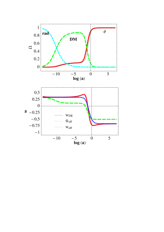
Figure 1: Evolution of the fractional energy densities ($\phi$, matter, radiation) in EF for the model $f(R)=R-\mu^{4}/R$ (top panel). Overimposed as dotted lines the evolution of $\tilde{\Omega}_{\phi}$ for $n=4$ and $10$. Notice the constant value $\tilde{\Omega}_{\phi}\simeq 1/9$ in the $\phi$MDE phase between radiation and DE domination. In the bottom panel we plot the evolution of the observed EOS $w_{\rm{DE}}$ of DE in JF and the effective EOS in both EF and JF ($n=1$).

As shown in BNST for all values of $n$ outside $(-1,0)$ the system has one and only one global attractor solution, a scalar-field dominated solution with an energy fraction $\widetilde{\Omega}_{\phi}=1$. This solution appears when the potential term in Eq. (5) dominates over the coupling term on the r.h.s., and is therefore independent of the coupling. On this attractor the scale factor evolves as $\tilde{a}\sim\tilde{t}^{2/[3(1+\tilde{w}_{\rm{eff}})]}$ where the effective equation of state (EOS) is $\tilde{w}_{\rm{eff}}=-1+\lambda^{2}/3=-1+\frac{2(2+n)^{2}}{9(1+n)^{2}}$. This can be identified with the acceleration today if $\mu\sim H_{0}$.

Beside the final attractor, a coupled field with an exponential potential has also another solution in which matter and field scale in the same way with time and, consequently, their density fractions are constants. This epoch has been denoted as $\phi$-matter-dominated era ($\phi$MDE) Luca1 . As we will show in a moment, the $\phi$MDE plays a central role in this work. This epoch occurs just after the radiation era and replaces the usual MDE. During the $\phi$MDE the energy fraction $\widetilde{\Omega}_{\phi}$ and the effective EOS $\widetilde{w}_{\rm{eff}}$ are constant and given by Luca1 ; BNST $\widetilde{\Omega}_{\phi}=\widetilde{w}_{\rm{eff}}=4\beta^{2}/9\,.$ Then we have $\widetilde{\Omega}_{\phi}=\widetilde{w}_{\rm{eff}}=1/9$ in $f(R)$ gravity theories, regardless of the form of $f(R)$. Therefore, contrary to standard cosmology, in coupled models DE is not negligible in the past (until the radiation era). In contrast to the accelerated attractor, the $\phi$MDE occurs when the coupling term in the r.h.s. of Eq. (5) dominates over the potential term, as it can be explicitly shown. This aspect is crucial for the present work since it implies that the $\phi$MDE exists independently of the form of $f(R)$. In this regime the scale factor behaves as $\tilde{a}\sim\tilde{t}^{3/5}$: in the JF this becomes $a\sim t^{1/2}$ instead of the usual $t^{2/3}$ behavior of the MDE. This is clearly a strong deviation from standard cosmology and, as one can expect, is ruled out by observations, as illustrated below. Notice that the JF evolution in this phase corresponds to $R=0$ as during the radiation epoch but, just as in that case, there is no singularity in an inverse power-law theory because this behavior is not exact (see below). In the language of dynamical systems, the $\phi$MDE is a saddle point.

To analyse numerically the full system (including the radiation energy density $\rho_{\rm{rad}}$ which obeys the standard conservation equation in both frames), we introduce the following quantities:

$$x_{1}=\frac{\kappa\phi^{\prime}}{\sqrt{6}},\quad x_{2}=\frac{\kappa}{\widetilde{H}}\sqrt{\frac{V}{3}},\quad x_{3}=\frac{\kappa}{\widetilde{H}}\sqrt{\frac{\rho_{\rm{rad}}}{3}},$$ (9)

where a prime denotes the derivative with respect to $N\equiv{\rm{log}}\,(\tilde{a})$. The energy fractions of the field $\phi$ and of matter are given by $\widetilde{\Omega}_{\phi}=x_{1}^{2}+x_{2}^{2}$ and $\widetilde{\Omega}_{m}=1-x_{1}^{2}-x_{2}^{2}-x_{3}^{2}$, respectively. The effective EOS and the field EOS are $\widetilde{w}_{\rm{eff}}=x_{1}^{2}-x_{2}^{2}+x_{3}^{2}/3$ and $\widetilde{w}_{\phi}=(x_{1}^{2}-x_{2}^{2})/(x_{1}^{2}+x_{2}^{2})$, respectively. The complete system has been already studied in Ref. Luca1 and we will not repeat it here. The $\phi$MDE corresponds to the fixed points $(x_{1},x_{2},x_{3})=(1/3,0,0)$ with $\widetilde{\Omega}_{\phi}=\widetilde{w}_{\rm{eff}}=1/9$. After this, the universe falls on the final attractor, which is the accelerated fixed point $(x_{1},x_{2},x_{3})=(\lambda/\sqrt{6},\sqrt{1-\lambda^{2}/6},0)$ with $\widetilde{\Omega}_{\phi}=1$ and $\widetilde{w}_{\rm{eff}}=-1+\lambda^{2}/3$.

To return to the JF we can simply apply the transformation law (4). In the regime where radiation is negligible ($x_{3}\simeq 0$) we obtain the following effective EOS

$$w_{\rm{eff}}=\frac{1}{3}-\frac{2n}{3(1+n)}\frac{x_{2}^{2}}{(1-x_{1})^{2}}\,,$$ (10)

together with the relation

$$\Omega_{m}\equiv\frac{\kappa^{2}\rho_{m}}{3H^{2}F}=\frac{\widetilde{\Omega}_{m}}{(1-x_{1})^{2}}.$$ (11)

For the accelerated attractor we have $w_{\rm{eff}}=-1+\frac{2(2+n)}{3(1+n)(1+2n)}$ (this relation was originally found in the context of inflation in coa ), which gives $w_{\rm{eff}}=-2/3$ for $n=1$. The $\phi$MDE corresponds to $x_{2}=0$ and therefore $w_{\rm{eff}}=1/3$ for any $n$, giving $a\propto t^{1/2}$. From Eq. (11) one has $\Omega_{m}=2$ and $\Omega_{\rm{R}}\equiv(RF-f-6H\dot{F})/6FH^{2}=-1$ in the $\phi$MDE [see Eq. (2)]. Since $\Omega_{\rm{R}}$ does not need to be positive definite, $\Omega_{m}$ can be larger than unity without any inconsistency.

Notice also that $w_{\phi}$ differs from the quantity $w_{DE}$ used to annalyse SN data and defined through the equation $H^{2}=H_{0}^{2}[\Omega_{m}^{(0)}a^{-3}+(1-\Omega_{m}^{(0)})a^{-3}\exp(-3\int{\rm{d}}a\,w_{\rm{DE}}/a)]$. We will also computte $w_{\rm{DE}}$ below.

Most modifications of gravity suggested in the literature consider terms in addition to the usual Einstein-Hilbert Lagrangian. For instance, several authors have studied the following DE model Capo ; Carroll :

$$f(R)=R-\mu^{2(n+1)}/R^{n}\,.$$ (12)

In this case the potential in EF is given by

$$V(\phi)=Ae^{-\frac{2\sqrt{6}}{3}\kappa\phi}(e^{\frac{\sqrt{6}}{3}\kappa\phi}-1)^{\frac{n}{n+1}},$$ (13)

which vanishes at $\phi=0$ and has a maximum at $\kappa\phi=2(n+1)/(n+2)$. In the limit $\phi\rightarrow\infty$ it behaves as $V(\phi)\propto\exp(-\lambda\kappa\phi)$. For negative $n$ the pure exponential approximation is always good during the past cosmic history if the higher-curvature term is responsible for the present acceleration, because we are always in large $R$ limit. For positive $n$ the potential (13) differs from the pure exponential one in the limit $R\gg\mu^{2}$ and one might expect that for these values the evolution goes on as in the standard case and, in particular, the $\phi$MDE disappears. However, we show now by building an explicit solution that in reality this does not happen.

Let us focus on the $R-\mu^{4}/R$ model taken for simplicity without radiation. During the $\phi$MDE one can approximate the scale factor in JF as $a(t)=(t/t_{i})^{1/2}+\epsilon(t)(t/t_{i})^{9/4}$ where $t_{i}$ is an initial time at the beginning of the $\phi$MDE. This solution is valid at first order in $\epsilon$ provided $\epsilon=(\mu^{2}/144H_{i}^{2})/((\rho_{m}^{(i)}/3H_{i}^{2})-\sqrt{H/H_{i}})^{1/2}$, which is indeed small for $\mu$ of order $H_{0}$ as present acceleration requires. After some time, the correction gets larger than the zero-th order term itself and the $\phi$MDE is followed by a phase of accelerated expansion. Then the beginning of the late-time acceleration is quantified by the condition $t\approx(144H_{i}^{2}\sqrt{(\rho_{m}^{(i)}/3H_{i}^{2})}/\mu^{2})^{4/7}\,t_{i}$. A similar argument applies for any $n<-1,n>-3/4$ with a correction growing as $t^{5/2-1/2(n+1)}$. Since $R$ is of order $\mu^{2}$ at the beginning of the $\phi$MDE, the term $\mu^{4}/R$ dominates over $R$ after the radiation era. This applies for any $\mu$, no matter how small. In other words, the limit $\mu\to 0$ of a fourth-order theory does not reduce to second-order general relativity if, at the same time, one imposes the conditions of acceleration today (cfr. Fa06 ).

For larger $\mu$ ($\gg H_{0}$) the $\phi$MDE can be shortened or bypassed from the above condition, but then DE dominates soon without a matter dominated epoch. Thus we have only two cases: either (i) the $\phi$MDE exists, or (ii) a rapid transition from the radiation era to the accelerating stage (without $\phi$MDE) takes place. In summary, the system never behaves as in a standard cosmological scenario except during radiation (during which matter and field play no role in the expansion rate). In other words, whenever matter is dynamically important, DE is also important as a consequence of the coupling. We now confirm all this by a direct numerical integration.

In Fig. 1 we plot the evolution of $\Omega_{\phi}$, $\Omega_{\rm{DM}}$ and $\Omega_{\rm{rad}}$ and the equation of state in EF for $n=1,4$ and $10$ and $\mu\approx H_{0}$. The present values of the radiation and matter density fractions are chosen to match the observations in JF. As expected, the system enters the $\phi$MDE after the radiation era and finally falls on the accelerated attractor. We ran our numerical code for other positive and negative values of $n$ (from $n=-10$ to $n=10$, limiting to the accelerating cases) and found similar cosmological evolutions. The plots in Fig. 1 are therefore qualitatively valid for any $R+\alpha R^{-n}$ model (provided $F>0$). It is also interesting to observe that the EOS is strongly varying with time just near $z=0$: this should serve as a reminder that a simple parametrization of $w_{{\rm DE}}$ may often fail to describe interesting cosmologies.

We can show now that an effective EOS $w_{\rm{eff}}=1/3$ during the $\phi$MDE is cosmologically unacceptable. In principle this should be shown case by case by a complete likelihood analysis of CMB and LSS data (see aq for such an analysis for various coupled models), but this program is hardly feasible if we want to make general statements on $f(R)$ theories. Instead we take a simpler but general approach. We calculate the angular size of the sound horizon

$$\theta_{s}=\int_{z_{\rm{dec}}}^{\infty}\frac{c_{s}(z){\rm{d}}z}{H(z)}\,/\int_{0}^{z_{\rm{dec}}}\frac{{\rm{d}}z}{H(z)}\,,$$ (14)

where $c_{s}^{2}(z)=1/[3(1+3\rho_{b}/4\rho_{\gamma})]$ is the adiabatic baryon-photon sound speed. According to the WMAP3y results WMAP , the currently measured value assuming a constant $w$ is $\theta_{s}=0.5946\pm 0.0021$ deg. As radiation follows the same conservation law, the thermal history is the same as in usual cosmology so that $z_{\rm{dec}}$ is unchanged. It is easy to show that the integrand ${\rm{d}}z/H(z)$ is conformally invariant. For the model (12) we integrate numerically the equations of motion in EF (including radiation) by changing initial conditions for $x_{1},x_{2},x_{3}$ via a trial and error procedure until we obtain a present universe with a JF matter and radiation densities as observed in the WMAP data (we used $\Omega_{m}^{(0)}=0.3$ and $h=0.7$). Once we have the full background solution we evaluate $\theta_{s}$ with $z_{\rm{dec}}$ obtained by solving the relation $\widetilde{z}_{\rm{dec}}e^{\kappa(\phi-\phi_{0})/\sqrt{6}}=z_{\rm{dec}}$. We have two competing effects: first, since the $\phi$MDE is more decelerated than in the usual case $r(z_{\rm{dec}})$ will be systematically smaller; second, the physical sound horizon distance at decoupling is smaller than in usual cosmology partly because in our models $a\propto t^{1/2}$ also between $t_{\rm{eq}}$ and $t_{\rm{dec}}$ with $z_{\rm{eq}}>z_{\rm{dec}}$ and mostly because $H(z)$ before decoupling is much higher than in the standard case. Assuming $H(z)=H_{0}(1+z)^{2}$ instead of $(1+z)^{3/2}$, $H(z_{dec})$ becomes 30 times larger than in standard models. We find that the second effect is by far the dominating one, and as a consequence $\theta_{s}$ turns out to be an order of magnitude smaller than the observed value. In practice, we find that $\theta_{s}$ can be approximated to a few percent using a standard cosmological model with an uncoupled dark energy component and a matter component with effective equation of state $w=1/3$. The typical values we find are near $\theta_{s}\approx 0.03$ deg, i.e. more than ten times smaller than in a standard model. The periodic spacing $\Delta\ell$ between the acoustic peaks in the CMB will be larger too by nearly the same factor.

In Fig. 2 we plot the value of $\theta_{s}$ as a function of the coupling constant $\beta$ (see eqs. 5-6) and for several $n$’s. Clearly there is no way that small changes in $\Omega_{m}^{(0)}$ or $h$ or $w_{\mathrm{eff}}$ can cure this problem. Discrepancies are found as well for the age of the universe which turns out to be near 10-11 Gyr. As to be expected, we also find that the perturbations depart significantly from the standard case (as in pure exponential coupled models aq ): for the matter density contrast on sub-horizon scales we find $\delta\sim a^{2}$ during $\phi$MDE instead of the standard linear law.

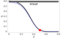
Figure 2: The sound horizon angular distance $\theta_{s}$ as a function of the coupling $\beta$ for $n=1$ (thick line) and $n=-2,3,10$ (dotted lines). The disk marks the value for $\beta=1/2$. The grayed region shows the WMAP3y constraint at $4\sigma$.

It is possible to generalize our results in several ways. First, one can show by direct substitution that the standard matter era $t^{2/3}$ is a solution of (2) only for pure power laws (plus possibly a cosmological constant) $R^{-n}$ with $n=-1,-(7\pm\sqrt{73})/12$. In the last two cases, however, the “matter” era occurs for $\Omega_{m}=0$ and is therefore unacceptable. The first case is clearly the pure Einstein case: this shows that a standard sequence of (exact) $t^{2/3}$ expansion followed by acceleration can occur only for $\Lambda$CDM. In contrast, the $\phi$MDE generically exists as a saddle point. For $R^{-n}$ with $-1<n<-3/4$ the $\phi$MDE is instead a stable point and the models are ruled out anyway. Still, this alone does not guarantee that the $\phi$MDE is always reached, regardless of the initial conditions, and a case-by-case numerical analysis is necessary. We explored extensively models like $f(R)=\exp(R)$ and $\log(R)$ and always found $\phi$MDE before acceleration. We also carried out a preliminary analysis of Lagrangians for the models like $f=R-c(R_{\mu\nu}R^{\mu\nu})^{-n}$, $f=R-c(R_{\alpha\beta\gamma\delta}R^{\alpha\beta\gamma\delta})^{-n}$ and $f=R-c(R_{{\rm GB}})^{-n}$ (where $R_{{\rm GB}}$ is a Gauss-Bonnet term) and did not find any acceptable cosmological evolution.

For the $f(R)=R-\mu_{1}^{4}/R+\mu_{2}R^{2}$ models, two mechanisms that could satisfy the local gravity constraints were suggested. One ON achieves a short interaction range (or a large field mass) by adjusting $\mu_{1},\mu_{2}$ so that ${\rm d}^{2}V(\phi)/{\rm d}\phi^{2}$ vanishes today, when $R=\sqrt{3}\mu_{1}^{2}$. Before this the $R^{2}$ term dominates and therefore we are back in one of our cases and the $\phi$MDE takes place. Moreover, we find that the local minimum in the EF potential for such a class of Lagrangians does not lead to a late-time (effective) cosmological constant. Another possibility to build a large mass is to take a very small $\mu_{2}$ brook , but in this case it is the $1/R$ term that dominates the cosmological evolution from the end of radiation, and again we are back in one of our cases. So even models that are designed to pass local gravity experiments fail our cosmological test. In summary, the main feature of our analysis is the modification of the standard matter dominated epoch for the $f(R)$ dark energy models investigated here. Hence these models are ruled out as viable cosmologies even if they are arranged to pass the Supernovae test and the local gravity constraints. We conjecture that our results apply to a much larger class of $f(R)$ models; the precise conditions that determine the cosmological behavior will be published in future works.

Acknowledgments– L. A. acknowledges the hospitality at the Gunma College of Technology and support from JSPS. The work of S. T. is supported by JSPS.

References

- (1) V. Sahni and A. A. Starobinsky, Int. J. Mod. Phys. D 9, 373 (2000); T. Padmanabhan, Phys. Rept. 380, 235 (2003); E. J. Copeland, M. Sami and S. Tsujikawa, hep-th/0603057.
- (2) S. Capozziello, V. F. Cardone, S. Carloni and A. Troisi, Int. J. Mod. Phys. D 12, 1969 (2003).
- (3) S. M. Carroll, V. Duvvuri, M. Trodden and M. S. Turner, Phys. Rev. D 70, 043528 (2004).
- (4) A. D. Dolgov and M. Kawasaki, Phys. Lett. B 573, 1 (2003); T. Chiba, Phys. Lett. B 575, 1 (2003).
- (5) P. Teyssandier and P. Tourrenc, J. Math. Phys. 24, 2793 (1983).
- (6) S. Nojiri and S. D. Odintsov, Phys. Rev. D 68, 123512 (2003).
- (7) A. W. Brookfield, C. v. de Bruck and L. M. H. Hall, hep-th/0608015.
- (8) A. A. Starobinsky, Phys. Lett. B 91, 99 (1980).
- (9) B. Boisseau, G. Esposito-Farèse, D. Polarski and A. A. Starobinsky, Phys. Rev. Lett. 85, 2236 (2000).
- (10) G. Esposito-Farèse and D. Polarski, Phys. Rev. D 63, 063504 (2001).
- (11) L. Amendola, Phys. Rev. D 62, 043511 (2000).
- (12) B. Gumjudpai, T. Naskar, M. Sami and S. Tsujikawa, JCAP 0506, 007 (2005); S. Tsujikawa, Phys. Rev. D 73, 103504 (2006).
- (13) S. Capozziello, F. Occhionero and L. Amendola, Int. J. Mod. Phys. D 1, 615 (1993).
- (14) V. Faraoni, Phys. Rev. D 74, 023529 (2006).
- (15) D.N. Spergel et al. [WMAP Collaboration], astro-ph/0603449
- (16) L. Amendola and C. Quercellini, Phys. Rev. D 68, 023514 (2003).