Gas metallicity diagnostics in star-forming galaxies

Generally the gas metallicity in distant galaxies can only be inferred by using a few prominent emission lines. Various theoretical models have been used to predict the relationship between emission line fluxes and metallicity, suggesting that some line ratios can be used as diagnostics of the gas metallicity in galaxies. However, accurate empirical calibrations of these emission line flux ratios from real galaxy spectra spanning a wide metallicity range are still lacking. In this paper we provide such empirical calibrations by using the combination of two sets of spectroscopic data: one consisting of low-metallicity galaxies with a measurement of [Oiii]$\lambda$4363 taken from the literature, including spectra from the Sloan Digital Sky Survey (SDSS), and the other one consisting of galaxies in the SDSS database whose gas metallicity has been determined from various strong emission lines in their spectra. This combined data set constitutes the largest sample of galaxies with information on the gas metallicity available so far and spanning the widest metallicity range. By using these data we obtain accurate empirical relations between gas metallicity and several emission line diagnostics, including the $R_{23}$ parameter, the [Nii]$\lambda$6584/H$\alpha$ and [Oiii]$\lambda$5007/[Nii]$\lambda$6584 ratios. Our empirical diagrams show that the line ratio [Oiii]$\lambda$5007/[Oii]$\lambda$3727 is a useful tool to break the degeneracy in the $R_{23}$ parameter when no information on the [Nii]$\lambda$6584 line is available. The line ratio [Neiii]$\lambda$3869/[Oii]$\lambda$3727 also results to be a useful metallicity indicator for high-$z$ galaxies, especially when the $R_{23}$ parameter or other diagnostics involving [Oiii]$\lambda$5007 or [Nii]$\lambda$6584 are not available. Additional, useful diagnostics newly proposed in this paper are the line ratios of (H$\alpha$+[Nii]$\lambda\lambda$6548,6584)/[Sii]$\lambda$6720, [Oiii]$\lambda$5007/H$\beta$, and [Oii]$\lambda$3727/H$\beta$. Finally, we compare these empirical relations with photoionization models. We find that the empirical $R_{23}$-metallicity sequence is strongly discrepant with respect to the trend expected by models with constant ionization parameter. Such a discrepancy is also found for other line ratios. These discrepancies provide evidence for a strong metallicity dependence of the average ionization parameter in galaxies. In particular, we find that the average ionization parameter in galaxies increases by $\sim 0.7$ dex as the metallicity decreases from 2 Z_⊙ to 0.05 Z_⊙, with a small dispersion. This result should warn about the use of theoretical models with constant ionization parameter to infer metallicities from observed line ratios.

1 Introduction

The gas metallicity is one of the most important tools to investigate the evolutionary history of galaxies. This is because the gas metallicity of galaxies is basically determined by their star-formation history. Recent observational studies allowed the investigation of the gas metallicity even in high-$z$ galaxies beyond $z=1$, such as Lyman-break galaxies (e.g., Teplitz et al. 2000a, 2000b; Pettini et al. 2001), submillimeter-selected high-$z$ galaxies (Swinbank et al. 2004), and so on (see also, e.g., Kobulnicky & Kewley 2004; Savaglio et al. 2005; Maier et al. 2006; Liang et al. 2006; Erb et al. 2006). Such observational insights on the metallicity evolution of galaxies are now giving constraints on the theoretical understandings of the formation and the evolution of galaxies (e.g., Bicker et al. 2004).

However, metallicity measurements in distant galaxies are not straightforward. Information on the gas temperature is required for a precise determination of the gas metallicity, but the gas temperature can be accurately inferred only when the fluxes of auroral emission lines such as [Oiii]$\lambda$4363 and [Nii]$\lambda$5755 are known, and these are generally too weak to be measured in faint distant galaxies. The measurement of the auroral emission lines is difficult even for galaxies in the local universe especially when the gas metallicity is high, because the collisional excitation of the auroral transitions is suppressed due to efficient cooling through far-infrared fine-structure emission lines (e.g., Ferland et al. 1984; Nagao et al. 2006a). Therefore, in general we have to rely on some relations between gas metallicity and flux ratios of strong emission-lines to estimate the gas metallicity in most galaxies. Extensive studies have been performed to calibrate such metallicity diagnostics by using only strong emission lines. One of the most frequently used metallicity diagnostics is the $R_{23}$ parameter, defined as

$$R_{23}\!=\!\frac{F({\rm[OII]}\lambda 3727)\!\!+\!\!F({\rm[OIII]}\lambda 4959)\!\!+\!\!F({\rm[OIII]}\lambda 5007)}{F({\rm H}\beta\lambda 4861)},$$ (1)

where $F$([Oii]$\lambda$3727), $F$([Oiii]$\lambda$4959) and so on denote the emission-line fluxes of [Oii]$\lambda$3727, [Oiii]$\lambda$4959 and so on, respectively. The $R_{23}$ was proposed by Pagel et al. (1979), and its calibration to the oxygen abundance has been improved by various photoionization model calculations (e.g., McGaugh 1991; Kewley & Dopita 2002).

One serious problem of this indicator is that a certain value of $R_{23}$ has two different solutions, a low-metallicity solution and a high metallicity one. Therefore additional, or alternative, diagnostics aimed at removing the $R_{23}$ degeneracy have been proposed (e.g., Alloin et al. 1979; Denicoló et al. 2002; Kewley & Dopita 2002; Pettini & Pagel 2004). However, most of these methods exploit the [Nii]$\lambda$6584 line, which has the problem of being very weak at sub-solar metallicities (hence difficult to measure) and the problem of being rapidly shifted outside the spectral band of many surveys at high redshift (e.g., unusable beyond $z\sim 0.5$ in optical spectra). On the theoretical side various models have been presented, which provide the ratios among the most prominent emission lines as a function of metallicity (e.g. Kewley and Dopita 2002). However, model predictions strongly depend on the assumed physical parameters of the ionized gas, and in particular on the ionization parameter [$U\equiv\Phi_{\rm H}/(cn_{\rm H})$, where $\Phi_{\rm H}$ is the surface flux of hydrogen-ionizing photon and $n_{\rm H}$ is the gas density]. As a consequence, an accurate correspondence between individual diagnostics (line ratios) and metallicity cannot be established, because of the lack of information on the physical conditions of the gas. Summarizing, many gas metallicity diagnostics proposed so far are either ambiguous or unusable when applied to the spectra of distant galaxies.

The goal of this paper is to obtain accurate, empirical calibrations between metallicity and individual diagnostics involving a few strong emission lines, which can be applied to the spectra of distant galaxies. In particular, we re-calibrate diagnostics already proposed in the past, but we also propose new diagnostics which appear particularly suited for distant galaxies. This work is obtained by combining two large data sets. The first one is composed of recent spectroscopic observations of low-metallicity galaxies [7.0$\la$12+log(O/H)$\la$8.5], whose metallicity is accurately determined through the [Oiii]$\lambda$4363 line (§§2.1). This dataset consists of two subsamples; one is taken from the database of the Sloan Digital Sky Survey (SDSS; York et al. 2000; Strauss et al. 2002) (§§2.1.1) and the other is taken from the literature (§§2.1.2). The second data set is a subsample of galaxies in the SDSS database, whose metallicity has been derived by Tremonti et al. (2004) [8.2$\la$12+log(O/H)$\la$9.2; see §§2.2]. These combined data sets provide the largest sample of galaxies with information on the gas metallicities and spanning more than 2 dex in metallicity.

2 Data

2.1 Spectroscopic data of low-metallicity galaxies with a [OIII]$\lambda$4363 measurement

2.1.1 SDSS data (sample A)

The gas-phase oxygen abundance is well determined when the flux of [Oiii]$\lambda$4363 is measured (e.g., Osterbrock 1989). Although such measurements have been performed for more than a hundred low-metallicity galaxies, simple compilation of those earlier results may introduce some unexpected biases and uncertainties. This is because the data were collected by various (heterogeneous) observations with different properties (aperture size, wavelength resolution, and so on) and because the method of calculating the oxygen abundance is different for different authors. Recently, Izotov et al. (2006b) reported their systematic measurements of the oxygen abundance for low-metallicity galaxies in the SDSS Data Release 3 (DR3; Abazajian et al. 2005) by using the [Oiii]$\lambda$4363 emission-line flux. The extinction-corrected emission-line fluxes of galaxies with a measurement of the oxygen abundance provided by Izotov et al. (2006b) are the ideal data for the empirical calibration of metallicity diagnostics, because the data were obtained and measured in a homogeneous way and because the oxygen abundance is also calculated with a common method. The number of spectra analyzed by Izotov et al. (2006b) is 309. Among them, we use the data with a relatively small error in the oxygen abundance [$\Delta$(log$\frac{\rm O}{\rm H})\leq$ 0.05] (146 spectra). Here we adopt the uncertainty [$\Delta$(log$\frac{\rm O}{\rm H}$)] given in Table 2 of Izotov et al. (2006). Since some spectra in the database of Izotov et al. (2006b) are duplicated for the same objects, the number of galaxies with $\Delta$(log$\frac{\rm O}{\rm H})\leq$ 0.05 is 139. Hereafter we call this sample “sample A”.

However, this sample has two problems when used to accurately calibrate metallicity diagnostics. First, most of galaxies in sample A have a relatively high oxygen abundance, and only 6 of them have 12+log(O/H) $<$ 7.6. Therefore the statistical reliability of the empirical calibration of metallicity diagnostics would be extremely poor at 12+log(O/H) $<$ 7.6 if using only this sample. Second, in sample A, there is the remarkable tendency for lower-metallicity galaxies to have lower redshift. In Figure 1, the oxygen abundance of galaxies in sample A is shown as a function of redshift. The origin of this apparent tendency is likely due to the fact that SDSS is not a volume-limited survey; that is, galaxies at higher redshift have preferentially higher luminosity, and thus higher metallicity. In particular, all of the galaxies with 12+log(O/H) $<$ 7.6 are at $z<0.02$. This means that the [Oii]$\lambda$3727 flux cannot be measured for the latter galaxies due to the limited wavelength coverage of the SDSS spectroscopy ($\lambda_{\rm obs}\ga 3800{\rm\AA}$). Therefore, if using only sample A, we could not calibrate the diagnostics involving [Oii]$\lambda$3727 [$R_{23}$ and $F$([Nii]$\lambda$6584)/$F$([Oii]$\lambda$3727)] in the metallicity range 12+log(O/H) $<$ 7.6. This is a serious problem, because $R_{23}$ is one of the most frequently used metallicity diagnostics and thus should be calibrated in a wide metallicity range. In conclusion, the accurate calibration of various metallicity diagnostics in a wide metallicity range cannot be achieved by using only sample A. We therefore collected additional data of [Oiii]$\lambda$4363-detected galaxies, which are described in the following subsection.

2.1.2 Other data from literature (sample B)

In order to increase the number of low-metallicity galaxies with a measurement of the oxygen abundance, we compiled the reddening-corrected emission-line flux data of galaxies with a [Oiii]$\lambda$4363 measurement from the literature. The sample of compiled galaxies is given in Table 1. For the objects whose spectroscopic properties have been reported by more than one paper independently, we chose the one with higher signal-to-noise ratio. When both the spectroscopic properties of the whole galaxy and of parts of it have been reported, we compiled both of them (e.g., Mrk 116). Consequently, the number of the compiled objects is 157. To minimize possible systematic errors owing to the different methods on the calculation of the oxygen abundance, we re-calculate their oxygen abundance by adopting the same method used for sample A (Izotov et al. 2006b). The re-calculated $R_{23}$ parameter, gas density of [Sii]-emitting region [$n_{\rm H}$(S⁺)], gas temperature of [Oiii]-emitting region [$t{\rm(O^{2+})}$] and oxygen abundance [$12+$log(O/H)] are given in Table 1, along with the reference to the data of the emission-line flux ratios. To calculate $R_{23}$, we did not use $F$([Oiii]$\lambda$4959) but calculate the ratio of [$F$([Oii]$\lambda$3727) + 1.327$\times$$F$([Oiii]$\lambda$5007)] $\!\!/\!$$F$(H$\beta$) since only the flux of [Oiii]$\lambda$5007 (without that of [Oiii]$\lambda$4959) is given in some reference papers.

To check whether our adopted method causes possible systematic difference in the oxygen abundance from the values given in the original references, we compare the oxygen abundances re-calculated by us and those given in the original papers in Figure 3. Apparently, there is no systematic difference between our results and the results given in the literature. The mean and the RMS of the difference, [12+log(O/H)${}_{\rm this\ work}$] – [12+log(O/H)_literature], are +0.001 and 0.041, respectively. This mean value of the difference is smaller than the typical error of the re-calculated oxygen abundance. Among the 157 objects given in Table 1 and plotted in Figure 3, we use only data with $\Delta$(log$\frac{\rm O}{\rm H})\leq$ 0.05. This constraint results in a sample of 120 objects, that is hereafter called “sample B”. Note that the mean and the RMS of the difference, [12+log(O/H)${}_{\rm this\ work}$] – [12+log(O/H)_literature], for sample B are –0.008 and 0.038. Again the mean value of the difference is smaller than the typical error on the oxygen abundance.

2.2 Spectroscopic data of high-metallicity galaxies (sample C)

For high-metallicity galaxies, we referred to the oxygen abundance derived by Tremonti et al. (2004), who derived the metallicities of $\sim$53000 galaxies in the SDSS database. They used the fluxes of many strong emission lines ([Oii]$\lambda$3727, H$\beta\lambda$4861, [Oiii]$\lambda$5007, H$\alpha$, [Nii]$\lambda$6584, [Sii]$\lambda$6717, and [Sii]$\lambda$6731) and comparing them with photoionization models (Ferland et al. 1998). Although they presented the results of their analysis on the spectra of the SDSS Data Release 2 (DR2; Abazajian et al. 2004), they also provide the results of their recent analysis on the spectra from Data Release 4 (DR4; Adelman-McCarthy et al. 2006) on their web site. Their estimate of the oxygen abundance does not rely only on a single metallicity diagnostic flux ratio, but uses all the optical prominent emission lines (see also, Charlot & Longhetti 2001; Brinchmann et al. 2004). Therefore, among galaxies without [Oiii]$\lambda$4363 flux, their sample is currently the best one in terms of both sample size and reliability.

The oxygen-abundance catalog of the SDSS DR4 galaxies contains 567486 objects. The objects in the catalog are classified into the five classes; “star-forming galaxies”, “low S/N star-forming galaxies”, “composite”, “active galactic nuclei (AGNs)”, and “unclassificable”. We referred only to the galaxies belonging the first class (141317 objects). The emission-line fluxes of these galaxies are obtained from the emission-line flux catalog of the SDSS DR4 galaxies provided on the same web site as the oxygen-abundance catalog. The emission-line fluxes given in this catalog were measured from the stellar-continuum subtracted spectra with the latest high spectral resolution population synthesis models by Bruzual & Charlot (2003), and thus more reliable than the flux data provided on the SDSS Data Archive Server. Since the emission-line fluxes given in their catalog are not corrected for dust extinction, we corrected them by using the Balmer decrement method with the reddening curve of Cardelli et al. (1989). We then removed the duplicated objects and the objects observed in some problematic plates (see the SDSS web page) from the cross sample of the oxygen-abundance catalog and the emission-line flux catalog. Then we select only objects satisfying all of the following five criteria:

1. The redshift is higher than 0.028.

2. Both H$\alpha$ and H$\beta$ emission lines have S/N $\geq$ 10.

3. log$\frac{F({\rm[OIII]\lambda 5007})}{F({\rm H\beta})}$ $>$ $\frac{0.61}{{\rm log}\frac{F({\rm[NII]\lambda 6584})}{F({\rm H\alpha})}-0.05}$ + 1.3.

4. The fiber aperture covers at least 20% of the total $g^{\prime}$-band photons.

5. The uncertainty on the estimated stellar mass is less than 0.5 dex (i.e., log$M_{97.5}$ – log$M_{2.5}$ $<$ 0.5, where $M_{97.5}$ and $M_{2.5}$ are the 97.5th and 2.5th percentile of probability distribution of the estimated stellar mass; see Kauffmann et al. 2003b for more details).

The first criterion ensures the accurate measurement of $F$([Oii]$\lambda$3727). The second criterion selects emission-line galaxies. The S/N values are taken from the emission-line flux catalog; however, the errors in this catalog are underestimated with a factor of $\sim$2 (see the web site for more details). The third criterion is required to reject AGNs from the sample, following Kauffmann et al. (2003a), although the AGN removal had been already examined in the process of checking the classification in the oxygen-abundance catalog mentioned above. The fourth criterion is required to avoid significant aperture effects on the flux ratios. Kewley et al. (2005) reported that the introduced systematic error of the metallicity determination reaches up to $\sim$40% when the fiber covers only 20% of the total $g^{\prime}$-band photons (see also Tremonti et al. 2004). The fifth criterion is not directly relevant to this study, but is required in our companion paper (Nagao et al. 2006b).

Note that in sample C we do not put constraints on $\Delta$(log$\frac{\rm O}{\rm H})$. This is to prevent sample C to be devoid of galaxies at metallicities 12+log(O/H) $<$ 7.6 so that sample C and sample A+B have some overlap in terms of metallicities. Indeed, due to the luminosity-metallicity relation, low metallicity galaxies in sample C are on average fainter and therefore tend to have larger errors. However, the averaged gas metallicities in sample C are most likely reliable even at low metallicities, thanks to the large number of objects in the sample. Our final sample of emission-line galaxies consists of 48497 objects, which is hereafter called “sample C”. The redshift distribution of galaxies in sample C is shown in Figure 4. Its median value is 0.085, while the mean and the RMS are 0.092 and 0.040, respectively. The distribution of the oxygen abundance of galaxies in sample C is shown in Figure 5. Its median value is 9.016, while the mean and the RMS are 8.976 and 0.166. The means and the RMSs of the oxygen abundance of samples A, B, and C are summarized in Table 2.

3 Results

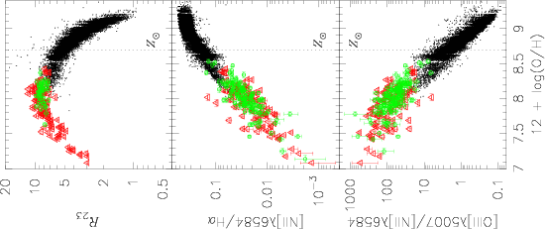
Figure 6: Emission-line flux ratios of $R_{23}$ (= [$F$([Oii]$\lambda$3727) + 1.327$\times$$F$([Oiii]$\lambda$5007)] $\!\!/\!$$F$(H$\beta$)), $F$([Nii]$\lambda$6584)/$F$(H$\alpha$), and $F$([Oiii]$\lambda$5007)/$F$([Nii]$\lambda$6584) for galaxies in sample A (red triangles), in sample B (green circles) and in sample C (black dots), as a function of the oxygen abundance. The compiled low-metallicity galaxies with an error of the oxygen abundance larger than 0.05 dex are not plotted. Dotted lines denote the solar metallicity [12+log(O/H) = 8.69].

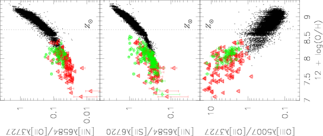
Figure 7: Same as Figure 6 but for the emission-line flux ratios of $F$([Nii]$\lambda$6584)/$F$([Oii]$\lambda$3727), $F$([Nii]$\lambda$6584)/$F$([Sii]$\lambda$6720), and $F$([Oiii]$\lambda$5007)/$F$([Oii]$\lambda$3727).

In Figures 6 and 7, we plot emission-line flux ratios for the galaxies in samples A, B, and C. To avoid noisy objects in sample C, we consider only those with S/N $\geq$ 10 (cataloged value) for all the related emission lines (e.g., H$\beta$, [Oii]$\lambda$3726, [Oii]$\lambda$3729 and [Oiii]$\lambda$5007 for the case of $R_{23}$). In addition to $R_{23}$, all the other flux ratios investigated here are metallicity-sensitive flux ratios and sometimes regarded as metallicity diagnostics (see, e.g., Kewley & Dopita 2002; Pettini & Pagel 2004; Kobulnicky & Kewley 2004). Among them, $F$([Oiii]$\lambda$5007)/$F$([Oii]$\lambda$3727) is sensitive also to the ionization parameter and thus it has not been regarded as a good metallicity diagnostic flux ratio (see Kewley & Dopita 2002). Instead, this flux ratio has been used to investigate the ionization parameter, and has been sometimes used in the following form:

$$O_{32}=\frac{F({\rm[OIII]}\lambda 4959)\!+\!F({\rm[OIII]}\lambda 5007)}{F({\rm[OII]}\lambda 3727)}$$ (2)

(e.g., Kobulnicky & Kewley 2004).

The data sequences in the diagnostics-metallicity diagrams are mostly continuous for different samples, and accordingly the whole sample shows clear relations between various metallicity diagnostics and the oxygen abundance. Since there are no apparent systematic differences in the diagnostics-metallicity sequences between sample A and sample B, we combined these two samples and identified as “sample A+B” hereafter in order to improve the statistics at low metallicities. The statistical properties of the sample A+B are given in Table 2. The diagram of $F$([Nii]$\lambda$6584)/$F$([Sii]$\lambda$6720) versus the oxygen abundance shows an apparent discontinuity between sample A+B and sample C, where $F$([Sii]$\lambda$6720) denotes the sum of $F$([Sii]$\lambda$6717) and $F$([Sii]$\lambda$6731). We will discuss the issue of this discontinuity in §§4.1.

The diagram of $R_{23}$ versus the oxygen abundance shows a $\cap$-shaped distribution with a peak at 12+log(O/H) $\sim$ 8.0. This is consistent with the previous studies on the empirical relation between $R_{23}$ and the oxygen abundance based on smaller samples of observational data (e.g., Edmunds & Pagel 1984; McGaugh 1991; Miller & Hodge 1996; Castellanos et al. 2002; Lee et al. 2003a; Bresolin et al. 2004, 2005; Pilyugin & Thuan 2005). As discussed in §§4.3, however, this appears to be systematically different from previous predictions of photoionization models.

To investigate the relation between the flux ratios and the oxygen abundances quantitatively, we calculate the means and the RMSs of the flux ratios of galaxies within bins of oxygen abundance. For sample A+B, we calculate them in the range $7.05<$ 12+log(O/H) $<8.55$ with a bin width of $\Delta$[log(O/H)] = 0.1, except at lowest and highest oxygen abundances, where the bin width is wider (i.e., $7.05<$ 12+log(O/H) $<7.45$ and $8.35<$ 12+log(O/H) $<8.55$) due to the small number of sources in these ranges. All of the metallicity bins contain at least 6 galaxies. The results are given in Table 3. We also calculate the mean and the RMS of flux ratios for sample C in the range $8.15<$ 12+log(O/H) $<9.25$ with a bin width of $\Delta$[log(O/H)] = 0.1 dex. The results are given in Table 4.

The calculated mean and the RMS of the flux ratios for each metallicity bin are shown in Figures 8 and 9. We then fit the observed sequences between flux ratios and oxygen abundance with polynomial functions in the range $7.05<$ 12+log(O/H) $<9.25$ (or $0.02<Z_{\rm gas}/Z_{\odot}<4$), and the results of the fits are also shown in Figures 8 and 9. We decided to fit 3rd-order polynomial functions for the binned data, not for the individual data, in order to avoid giving too much weights to the high metallicity range (where most of the data are). In Table 5, the coefficients of the best-fit polynomial functions are provided, according to the formula

$${\rm log}\ (F_{1}/F_{2})=\sum_{N}{a_{N}[{\rm log}(Z/Z_{\odot})]^{N}}$$ (3)

where $F_{1}/F_{2}$ is the line flux ratio (or the $R_{23}$ parameter) and $N=$ (0, 1, 2, 3). Here we adopt 12+log(O/H)_⊙ = 8.69 for $Z_{\odot}$ (Allende Prieto et al. 2001). For the convenience of the reader, in Table 6 we also give the coefficients of the best-fit polynomial functions in the following form:

$${\rm log}\ (F_{1}/F_{2})=\sum_{N}{b_{N}[12+{\rm log(O/H)}]^{N}}.$$ (4)

The expected uncertainties on the derived metallicities from the diagnostic flux ratios calibrated here can be estimated using the RMS values of the flux ratios given for each mass bin (Tables 3 and 4). By looking at the RMS plotted in Figures 8 and 9, we can recognize that, for instance, the diagnostic flux ratios give highly uncertain metallicities when $F$([Nii]$\lambda$6584)/$F$([Oii]$\lambda$3727) $\la$ 0.05, $F$([Oiii]$\lambda$5007)/$F$([Oii]$\lambda$3727) $\ga$ 2, and $F$([Nii]$\lambda$6584)/$F$([Sii]$\lambda$6720) $\la$ 0.3. On the contrary, the metallicity is well determined ($\Delta Z\la 0.2$ dex) when $F$([Oiii]$\lambda$5007)/$F$([Nii]$\lambda$6584) $\la$ 10 and $F$([Nii]$\lambda$6584)/$F$([Oii]$\lambda$3727) $\ga$ 0.05.

Finally we recall that these relations are valid only in the range 7.05 $<$ 12+log(O/H) $<$ 9.25 (which is however much wider than in any previous work). We warn on the use of these relations outside such metallicity range, since it would rely only on their extrapolation.

4 Discussion

4.1 Consistency between sample A+B and sample C

Before interpreting the results, we discuss on the consistency of the two main samples, i.e., galaxies with (A+B) and without (C) [Oiii]$\lambda$4363 measurements. As mentioned in §3, the relation between some emission-line flux ratios and the oxygen abundance is not smoothly connected between the two samples (A+B and C), and this is especially significant for the flux ratios of $F$([Oiii]$\lambda$5007)/$F$([Oii]$\lambda$3727) and $F$([Nii]$\lambda$6584)/$F$([Sii]$\lambda$6720), but is also seen in other cases (Figures 8 and 9). One of the possible reasons for this discrepancy is a systematic error in the estimate of the oxygen abundance for one (or both) of the two different methods, which in one case consists in using the gas temperature inferred through [Oiii]$\lambda$4363 emission (see §§2.1) and in the other case is using all of optical strong emission lines (Tremonti et al. 2004).

Kobulnicky et al. (1999) investigated a possible systematic error in the former method, that is, the gas temperature may be overestimated through the [Oiii]$\lambda$4363 emission and thus the oxygen abundance may tend to be underestimated accordingly. This is because the strength of the [Oiii]$\lambda$4363 emission significantly depends on the gas temperature and thus spectra obtained by a global aperture toward a galaxy are biased towards higher gas-temperature Hii regions (see also Peimbert 1967). According to their analysis, the overestimation of the gas temperature could be more serious in low-metallicity systems and could reach up to $\Delta T_{\rm e}=1000-3000$K, which results in the systematic underestimation of the oxygen abundance of 0.05 – 0.2 dex. However, although this effect may partly account for the discrepancy of the metallicity dependence of $F$([Nii]$\lambda$6584)/$F$([Sii]$\lambda$6720), it goes in the opposite direction to account for the discrepancy seen in $F$([Oiii]$\lambda$5007)/$F$([Nii]$\lambda$6584) and $F$([Oiii]$\lambda$5007)/$F$([Oii]$\lambda$3727). Therefore, the effect of the biased temperature measurement is not the dominant origin of the discontinuities seen in Figures 8 and 9.

A systematic error in the oxygen abundance may exist in the method of Tremonti et al. (2004). They estimated the oxygen abundance by comparing photoionization models with some optical emission-line fluxes, which were measured on the spectra after subtraction of the stellar component. Although their method of the stellar-component subtraction is a sophisticated one and uses the most recent population synthesis models of Bruzual & Charlot (2003), it is not clear whether the measurement of emission lines lying on the deep and complex stellar absorption features is completely free from some possible systematic errors. A possible improper subtraction of the stellar absorption features may lead to systematic errors on the fluxes of Balmer lines, which might result in a systematic error in the estimation of the gas metallicity of galaxies in sample C. The subtraction of stellar absorption features may be inaccurate also in sample A+B. For instance, in some earlier works the stellar subtraction was performed by simply assuming $EW$(H$\beta$)_abs = 1${\rm\AA}$. This over-simplified assumption may introduce systematic errors in the derived gas metallicity and the emission-line flux ratios given in Table 1. Another possible source of uncertainty in the method of Tremonti et al. (2004) is the use of the [Nii]$\lambda$6584 flux and its comparison to models. Most photoionization models assume that the relative nitrogen abundance scales with the metallicity linearly when the primary nitrogen creation dominates, and scales quadratically when the secondary nitrogen creation is dominant. However, the transition metallicity between the two modes is uncertain. An inaccurate value of the transition metallicity (which is indeed uncertain) may lead to systematic errors in the estimation of metallicity especially at low metallicities, which could be one of the possible origin of the discrepancy seen in Figures 8 and 9.

The discrepancy in the metallicity dependences of emission-line flux ratios may also be a consequence of the selection of spectroscopic targets. While galaxies in sample C are basically selected in terms of their apparent magnitude and thus not largely biased toward any specific population, galaxies in sample B could be biased toward very strong emission-line galaxies (galaxies in sample A are in a composite situation; see Izotov et al. 2006). This is because the motivation behind most of the original observations, such as the studies on the primordial helium abundance (see the original references given in Table 1), required very accurate measurements of emission-line flux ratios. For a given metallicity, galaxies with stronger emission lines tend to be characterized by a higher ionization parameter, which may result into larger flux ratios of $F$([Oiii]$\lambda$5007)/$F$([Nii]$\lambda$6584) and $F$([Oiii]$\lambda$5007)/$F$([Oii]$\lambda$3727), although the difference in the ionization parameter should not cause a significant difference in the ratio of $F$([Nii]$\lambda$6584)/$F$([Sii]$\lambda$6720). We will discuss the effect of the ionization parameter on the discrepancy further in §§4.3.

Actually some or all of the above matters could contribute to the discontinuity in the metallicity dependences of emission-line flux ratios, and their discrimination or their accurate correction are not feasible. We thus simply adopt the results of the fit described in §3 and not take the effects of the possible systematic errors into account in the following discussion. However, it should be noted that this rather complex situation is caused by relying on two independent methods to measure the oxygen abundance. This problem will be solved if a large sample of galaxies with a wide range of the oxygen abundance is investigated by using a unique method throughout the concerned metallicity range.

4.2 Comparison with previous empirical calibrations

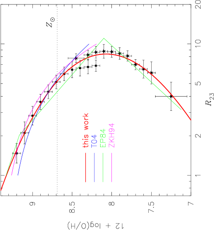
Figure 10: Comparison of our results with the previous empirical metallicity calibrations for the $R_{23}$ parameter. Solid red line denotes our calibration. Blue, green, and magenta lines denote the calibration given by Tremonti et al. (2004), Edmunds & Pagel (1984), and Zaritsky et al. (1994), respectively. Symbols and errorbars are the same as those in Figure 8. Vertical dotted line denotes the solar metallicity [12+log(O/H) = 8.69].

We compare the results of our calibrations with previous empirical calibrations. In particular, in Figure 10, we compare the empirical calibrations of $R_{23}$ derived by us with those obtained by Tremonti et al. (2004), Edmunds & Pagel (1984), and Zaritsky et al. (1994). While there is a reasonable agreement between our result and the result from previous calibration for the lower branch (Edmunds & Pagel 1984), there are some systematic discrepancies for the upper branch. We should in particular discuss the difference between our calibration and that of Tremonti et al. (2004), since our calibration in the high-metallicity range is based on the metallicity of the SDSS galaxies (in sample C) derived by Tremonti et al. (2004). The calibration by Tremonti et al. (2004), which is provided only for the upper branch, is clearly flatter than ours. This discrepancy may be ascribed to the combination of various possible factors. Our calibration also includes the fit of the new sample of [Oiii]$\lambda$4363-detected galaxies, which are not included in Tremonti et al. (2004), and this is certainly one of the reasons for the discrepancy. However, the latter issue cannot completely account for the discrepancy, since the Tremonti et al. (2004) calibration fails to reproduce the SDSS data at 12+log(O/H) $<$ 8.5 (as shown in Figure 10). It is likely that an additional source of the discrepancy is the different strategy of fitting the analytical function to the data. While we fit the third polynomial function to the binned data, Tremonti et al. (2004) fit the function to the whole sample of individual SDSS galaxies. Since the number of high metallicity galaxies [12+log(O/H) $>$ 8.5] is much larger than the low metallicity sub-sample [12+log(O/H) $<$ 8.5] as shown in Figure 5, the analytical fit of Tremonti et al. (2004) is dominated by the high-metallicity part of the $R_{23}$ diagram. Finally, the modest discrepancy at high metallicities [12+log(O/H) $>$ 9] may be partly attributed to the difference in the sample selection criteria. As described in §3, we select the galaxies in the sample C with S/N $\geq$ 10 for all of the lines H$\beta$, [Oii]$\lambda$3726, [Oii]$\lambda$3729, and [Oiii]$\lambda$5007 (note that the [Oii] doublet lines are measured separately in the original catalog we used), while Tremonti et al. (2004) adopted the S/N criteria only for H$\beta$, H$\alpha$ and [Nii]$\lambda$6584, not for [Oii]$\lambda$3726, [Oii]$\lambda$3729, and [Oiii]$\lambda$5007. Our selection criteria may preferentially reject objects at high metallicities with respect to those of Tremonti et al. (2004), because forbidden lines such as [Oii] and [Oiii] become weak when gas metallicity is high due to the suppressed collisional excitation mechanism (e.g., Ferland et al. 1984; Nagao et al. 2006a). This effect may result in our selective choice of objects with strong [Oii] and [Oiii] emission in a given metallicity bin, which could make our calibration to be steeper at high metallicities. Since the difference in the calibration between ours and that of Tremonti et al. (2004) is significant at 12+log(O/H) $>$ 9, it is suggested that our calibration for the $R_{23}$ may overestimate the gas metallicity at 12+log(O/H) $>$ 9 by a factor of $\Delta Z\sim 0.1$ dex at 12+log(O/H) $\sim$ 9.1.

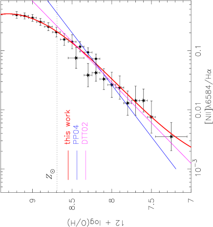
Figure 11: Comparison of our results with the previous empirical metallicity calibrations for $F$([Nii]$\lambda$6584)/$F$(H$\alpha$). Solid red line denotes our calibration. Blue and magenta lines denote the calibration given by Pettini & Pagel (2004) and Denicoló et al. (2002), respectively. Symbols and errorbars are the same as those in Figure 8. Vertical dotted line denotes the solar metallicity [12+log(O/H) = 8.69].

The calibration of the diagnostic flux ratio $F$([Nii]$\lambda$6584)/$F$(H$\alpha$) is especially important, because wavelength separation of the two lines is small (i.e., not sensitive to dust reddening and requiring only small wavelength coverage) and thus it is used as a diagnostic of the gas metallicity of galaxies at $z\la 2$ (e.g., Erb et al. 2006). In Figure 11, we compare the empirical calibrations of $F$([Nii]$\lambda$6584)/$F$(H$\alpha$) derived by us, with those derived by Pettini & Pagel (2004) and Denicoló et al. (2002). Our result agree reasonably well with Denicoló et al. (2002) only at sub solar metallicity, and there is a systematic difference in the slope between our result and the result reported by Pettini & Pagel (2004). The latter discrepancy may be due to the reduced metallicity range of the sample of Pettini & Pagel (2004), indeed most of their objects are distributed within 7.7 $<$ 12+log(O/H) $<$ 8.5. However, the difference is significant ($\Delta Z\ga 0.2$ dex) only at metallicities 12+log(O/H) $<$ 7.5 and 12+log(O/H) $>$ 8.5. Although the difference in the lowest-metallicity range is not a serious problem (because in this metallicity range the expected [Nii]$\lambda$6584 flux is extremely weak and thus its measurement would be very challenging and probably inaccurate), it is important to pay attention to the difference in the high-metallicity range. Note that such “high-metallicity” range (where the discrepancy with Pettini & Pagel 2004 occurs) is not so metal rich — the metallicity 12+log(O/H) = 8.5 corresponds to $Z=0.65Z_{\odot}$, still in the sub-solar metallicity domain.

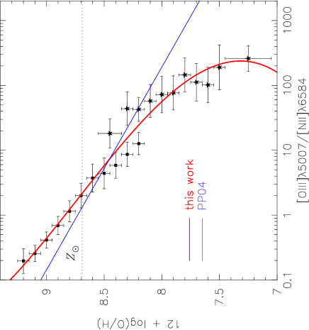
Figure 12: Comparison of our results with the previous empirical metallicity calibrations for $F$([Oiii]$\lambda$5007)/$F$([Nii]$\lambda$6584). Solid red line denotes our calibration, and blue line denotes the calibration given by Pettini & Pagel (2004). Symbols and errorbars are the same as those in Figure 8. Vertical dotted line denotes the solar metallicity [12+log(O/H) = 8.69].

In Figure 12, we compare the empirical calibrations of $F$([Oiii]$\lambda$5007)/$F$([Nii]$\lambda$6584 derived by us with the one derived by Pettini & Pagel (2004). The difference between the two calibrations is more serious than that seen in Figure 11 in the low metallicity range, 12+log(O/H) $<$ 8. However Pettini & Pagel (2004) correctly mentioned that the flux ratio $F$([Oiii]$\lambda$5007)/$F$([Nii]$\lambda$6584 is of little use when $F$([Oiii]$\lambda$5007)/$F$([Nii]$\lambda$6584 $\ga$ 100 because of the saturation of this diagnostic. The behavior of this diagnostic flux ratio in the low-metallicity range would be important to derive the upper limits on the metallicity from an upper limit of the [Nii]$\lambda$6584 flux.

4.3 Comparison with photoionization models

To interpret the metallicity dependences of the emission-line flux ratios, we compare observational data with the predictions of photoionization models. In Figures 13 and 14, we show the empirical metallicity dependences and the theoretical metallicity dependences of some metallicity diagnostics, where the latter are taken from Kewley & Dopita (2002) except for $F$([Nii]$\lambda$6584)/$F$(H$\alpha$) that is taken from Kobulnicky & Kewley (2004). Since the explicit analytic expression for the metallicity dependence of $F$([Oiii]$\lambda$5007)/$F$([Oii]$\lambda$3727) is not given by Kewley & Dopita (2002), we derive the polynomial expression of the theoretical metallicity dependence by fitting the results given in Table 2 of Kewley & Dopita (2002). The photoionization models presented by Kewley & Dopita (2002) and Kobulnicky & Kewley (2004) were calculated by the photoionization code MAPPINGS III (Sutherland & Dopita 1993) combined with the stellar population synthesis codes PEGASE (Fioc & Rocca-Volmerange 1997) and STARBURST99 (Leitherer et al. 1999), for the range $7.6<$ 12+log(O/H) $<9.4$. They assume that stars and gas have the same metallicity, which is a reasonable assumption given that photoionization is due to hot, young stars, presumably recently formed from the same gas that they are photoionizing. In their calculations, nitrogen is assumed to be a secondary nucleosynthesis element at 12+log(O/H) $>$ 8.3, and a primary nucleosynthesis element at lower metallicity. Effects of dust grains on the depletion of gas-phase heavy elements and on the radiative transfer are consistently taken into account. Their calculations cover the range of ionization parameters $-3.8\leq{\rm log}\ U\leq-2.0$, or equivalently, $5\times 10^{6}{\rm cm\ s}^{-1}\leq q\leq 3\times 10^{8}{\rm cm\ s}^{-1}$ (where $U\equiv q/c$). See Kewley & Dopita (2002) for details on the calculations. Note that they adopted 12+log(O/H)_⊙ = 8.93 (Anders & Grevesse 1989) and expressed the metallicity in units of $Z_{\odot}$ (12+log(O/H)_⊙ = 8.93). However, since we adopt a more recent value for the solar abundance, 12+log(O/H)_⊙ = 8.69 (Allende Prieto et al. 2001), the metallicity notation is different when the $Z_{\odot}$ unit is used, which should be kept in mind to compare our results with their predictions.

The most remarkable matter in the comparison between the empirical and theoretical metallicity dependences of emission-line flux ratios is the significant discrepancy in the theoretically-expected $R_{23}$-sequence with respect to the observed trend. This is especially significant at low metallicity range 12+log(O/H) $<$ 8. Shi et al. (2006) also recently reported that a previous theoretical calibration of $R_{23}$ (see McGaugh 1991; Kobulnicky et al. 1999) overpredicts the gas metallicity with respect to the metallicity measured through the gas temperature determined with [Oiii]$\lambda$4363 line ($\Delta Z\sim 0.2$ dex), especially in the low metallicity range [i.e., 12+log(O/H) $<$ 8]. This discrepancy is not due to an improper compilation in our data, because it has been reported also in the earlier works that the empirical peak of $R_{23}$ is seen around 12+(O/H) $\sim$ 8.0, as mentioned already in §3. The discrepancy cannot be ascribed to problems to the model results of Kewley & Dopita (2002) either, because other theoretical works also predict higher peak metallicity of $R_{23}$ independently [12+log(O/H) $\ga$ 8.3; e.g., Kobulnicky et al. 1999]. One possible idea to reconcile this discrepancy is that the ionization parameter of the gas is higher than the parameter range which Kewley & Dopita (2002) covers, especially in low-metallicity objects. If the ionization parameter correlates negatively with the gas metallicity and it reaches up to log $U>-2$ at the lowest metallicities, photoionization models would predict larger values of $R_{23}$ in the lower-metallicity range with respect to constant-$U$ models. This idea appears to be consistent with the behaviors of the empirical sequences in the $U$-sensitive flux ratios, $F$([Oiii]$\lambda$5007)/$F$([Nii]$\lambda$6584) (Figure 13) and $F$([Oiii]$\lambda$5007)/$F$([Oii]$\lambda$3727) (Figure 14). By focusing on these two $U$-sensitive flux ratios, we can see that the ionization parameter increases by $\sim$0.7 dex with decreasing oxygen abundance from 12+log(O/H) = 9.0 to 7.5, supporting the above interpretation. Although the absolute value of the required ionization parameter appear to be inconsistent between $R_{23}$ and the latter two $U$-sensitive flux ratios, the inferred absolute $U$ values depends also on some model assumptions such as the spectral energy distribution (SED) of ionizing photons or the relative elemental abundance ratios, which also change as a function of metallicity. We thus conclude that the metallicity dependence of the ionization parameter (hereafter “$U$-$Z$ relation”) causes the discrepancy between the empirical $R_{23}$ distribution and the model predictions with a constant ionization parameter.

Note that the $F$([Oiii]$\lambda$5007)/$F$([Nii]$\lambda$6584) and $F$([Oiii]$\lambda$5007)/$F$([Oii]$\lambda$3727) ratios are also sensitive to the hardness of the ionizing radiation, which is a strong function of the stellar metallicity. This effect can in principle also contribute to the dependence of $F$([Oiii]$\lambda$5007)/$F$([Nii]$\lambda$6584) and $F$([Oiii]$\lambda$5007)/$F$([Oii]$\lambda$3727) ratios on metallicity. However, the models by Kewley & Dopita (2002) plotted in Figures 13 and 14 already take into account the hardening of the stellar spectra as a function of metallicity. Therefore, the discrepancy between constant-$U$ models and the data indicates that the hardening of the ionizing spectra must be associated with a variation of $U$ with metallicity. In particular, the dependence of the $F$([Oiii]$\lambda$5007)/$F$([Oii]$\lambda$3727) ratio on metallicity cannot entirely be ascribed only to the hardening of the ionizing radiation, but also to a $U$-$Z$ relation.

The inferred $U$-$Z$ relation is a very interesting result. Maier et al. (2006) also recently reported that the lower-metallicity galaxies tend to be characterized by a higher ionization parameter (see also Maier et al. 2004, who reported the correlation between the absolute $B$ magnitude and the flux ratio of $F$([Oiii]$\lambda$5007)/$F$([Oii]$\lambda$3727) among galaxies in the local universe). Although a detailed theoretical interpretation of this empirical relation goes beyond the scope of this paper, in the following we discuss two possible qualitative interpretations. One possible origin of this effect may be associated with the mass–metallicity relation and with the mass–age relation in local galaxies. According to these relations, higher metallicity galaxies are associated with more massive and older systems. Hii regions ionized by later stellar populations are expected to be characterized by lower ionization parameters, due to the lower luminosity of the ionizing stars. Another possible explanation may be the (plausible) relation between gas metallicity and stellar metallicity, and in particular that lower metallicity gas is ionized by lower metallicity stars. For a given stellar mass, lower metallicity stars emit a harder and stronger radiation field, therefore giving a higher ionization parameter. The latter effect would naturally yield a $U$-$Z$ relationship. The former are just qualitative interpretations. However, a thorough investigation of this phenomenon will requite detailed observational studies of stellar population in star forming galaxies.

The comparison of the empirical and the theoretical sequences of the two $U$-sensitive diagnostic flux ratios, $F$([Oiii]$\lambda$5007)/$F$([Nii]$\lambda$6584) and $F$([Oiii]$\lambda$5007)/$F$([Oii]$\lambda$3727), also suggests the fact that the dispersion of the ionization parameter for a given metallicity should be relatively small. The typical RMS of the two flux ratios are $\sim$0.5 (in logarithm) at 12+log(O/H) $\sim$ 7.5. This corresponds to an RMS of the ionization parameter of $\sim$0.5 dex. This is the reason why the very $U$-sensitive flux ratio, $F$([Oiii]$\lambda$5007)/$F$([Oii]$\lambda$3727), shows a clear metallicity dependence as seen in Figure 13. The $U$-metallicity relationship is also important to understand the behavior of the empirical metallicity dependence of the flux ratio $F$([Oiii]$\lambda$5007)/$F$([Nii]$\lambda$6584). This flux ratio is predicted to decrease with the oxygen abundance below 12+log(O/H) $\sim$ 7.6 by photoionization models with a constant ionization parameter. Owing to the metallicity dependence of the ionization parameter, this flux ratio does not show the “turnover” seen in $R_{23}$ and thus it is very useful to investigate the gas metallicity of galaxies without the measurement of $F$([Oiii]$\lambda$4363). Another implication of these results is that one should not use constant-$U$ photoionization models to derive the oxygen abundance from the observed flux ratios, not only from $F$([Oiii]$\lambda$5007)/$F$([Nii]$\lambda$6584 but also from any other metallicity diagnostics, which introduce systematic errors in the calibration. The empirical relations provided in this paper (Tables 5 and 6) are very useful to avoid such systematic errors to derive the gas metallicity by using only strong emission lines.

As for the $U$-insensitive diagnostic flux ratios, $F$([Nii]$\lambda$6584)/$F$(H$\alpha$), $F$([Nii]$\lambda$6584)/$F$([Oii]$\lambda$3727) and $F$([Nii]$\lambda$6584)/$F$([Sii]$\lambda$6720), there are no significant discrepancies between the empirical sequence and the theoretical sequence (with a constant ionization parameter). This indirectly supports the above interpretation that the apparent discrepancy in $R_{23}$ between the empirical sequence and the results of photoionization model is caused by the effect of the ionization parameter. Note that there is little or no metallicity dependence of the flux ratios of $F$([Nii]$\lambda$6584)/$F$([Oii]$\lambda$3727) and $F$([Nii]$\lambda$6584)/$F$([Sii]$\lambda$6720) in the low-metallicity range, 12+log(O/H) $\la$ 8.0, in terms both of empirical and theoretical dependences. Therefore these diagnostic flux ratios are useful only for the high metallicity galaxies.

The photoionization models presented in Figures 13 and 14 suggest an additional interpretation of the discrepancy in some diagnostics between the two samples discussed in §§4.1 (i.e., the discontinuity between sample A+B and sample C). Focusing on the metallicity range of 12+log(O/H) $\sim$ 8.3 where the two datasets of sample A+B and sample C overlap, we note that the trend of the discrepancy suggests that the galaxies in sample A+B have higher ionization parameter than the galaxies in sample C. This supports the interpretation that the discrepancy is at least partly caused by the selection effect, i.e., galaxies with higher ionization parameter are selectively picked up in sample A+B. Then, what causes this selection effect? This may be related with the fact that the [Oiii]$\lambda$4363 emission is extremely weak in higher metallicity galaxies. This means that we can measure the [Oiii]$\lambda$4363 flux of galaxies with 12+log(O/H) $\sim$ 8.3 (the highest metallicity in the galaxies in sample A+B) only when the [Oiii] emission is very strong, which corresponds to a very high ionization parameter.

4.4 Implications for studies of high-redshift galaxies and new diagnostics

Although the $R_{23}$ method is thought to be a good metallicity diagnostic, various other diagnostics (some of which are investigated in this paper) have been proposed up to now. Indeed one of the main problems of the $R_{23}$ method is that there are two solutions for a given $R_{23}$ value and thus one cannot obtain a unique metallicity solution. Most of the newly proposed diagnostics use the [Nii]$\lambda$6584 line to remove the degeneracy in $R_{23}$, because the secondary nucleosynthesis of nitrogen makes this line emission very sensitive to the gas metallicity. However, there are two non-negligible problems with the use of the [Nii]$\lambda$6584 line. First, especially for low-metallicity systems, the contribution of the primary nucleosynthesis and the secondary nucleosynthesis in the nitrogen abundance is not well understood, which leads to an uncertainty in the relative nitrogen abundance as a function of the metallicity. Second, the [Nii]$\lambda$6584 emission is in the red part of the rest-frame optical spectrum of galaxies, which prevents its application to the observational investigations of high-$z$ systems. For example, the optical detectors with a sensitivity up to $\lambda\sim 1\mu$m can detect the [Nii]$\lambda$6584 emission of galaxies only at $z\la 0.52$, and the $K$-band atmospheric window limits the highest redshift to $z\sim 2.7$ for ground-based facilities. Although one of the undoubtfully interesting targets for the JWST is the population related to the cosmic reionization, the sensitivity of NIRSpec (Posselt et al. 2004) boarded on JWST can examine the [Nii]$\lambda$6584 emission of the objects at $z\la 6.6$, where the cosmic reionization has already nearly ended (e.g., Kashikawa et al. 2006; Fan et al. 2006). Another problem associated with the [Nii]$\lambda$6584 line is that it becomes very weak and difficult to measure at low metallicities: [Nii]$\lambda$6584/H$\alpha$ $<$ 0.1 at 12+log(O/H) $<$ 8.5.

Our results on the empirical metallicity dependences suggest that one does not need [Nii]$\lambda$6584 any more to distinguish the upper- and lower-branches of the $R_{23}$ sequence. This is because the flux ratio of $F$([Oiii]$\lambda$5007)/$F$([Oii]$\lambda$3727) is also a good metallicity diagnostics, thanks to the small dispersion of the ionization parameter at a given metallicity. The empirical $R_{23}$ sequence peaks at 12+log(O/H) $\sim$ 8.0, where the empirically determined flux ratio of $F$([Oiii]$\lambda$5007)/$F$([Oii]$\lambda$3727) is $\sim$2. Therefore one can recognize whether the observed $R_{23}$ belongs to the upper-branch of the $R_{23}$ sequence or not, depending on whether $F$([Oiii]$\lambda$5007)/$F$([Oii]$\lambda$3727) $<$ 2 or not. Note that this result is consistent with an earlier remark by Maier et al. (2004) that the flux ratio of $F$([Oiii]$\lambda$5007)/$F$([Oii]$\lambda$3727) can be used to distinguish the upper- and lower-branches of the $R_{23}$ sequence. Our work gives the physical explanation for this idea (the $U$-$Z$ relation) and a criterion to distinguish the degeneracy [$F$([Oiii]$\lambda$5007)/$F$([Oii]$\lambda$3727) $<$ 2] on the remark by Maier et al. (2004).

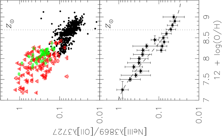
Figure 15: ($Upper$) Emission-line flux ratios of $F$([Neiii]$\lambda$3869)/ $F$([Oii]$\lambda$3727) of the galaxies in sample A (red triangles), those in sample B (green circles), and those in sample C (black dots), as a function of the oxygen abundance. As for sample C, only the objects with S/N([Neiii]) $>$ 10 and S/N([Oii]) $>$ 10 (cataloged values) are plotted. ($Lower$) Same as the upper panel but the mean and the RMS values are shown for each bin of the oxygen abundance, instead of the individual data. Filled stars and filled squares denote the mean flux ratios for galaxies in sample A+B and those for galaxies in sample C, respectively. The errorbar denotes the RMS for each metallicity bin. The dashed line denotes the best-fit polynomial (second-order) function.

The above result is due to the fact that the ionization parameter has a strong metallicity dependence, and it thus implies that the ionization parameter itself is a sort of metallicity diagnostic. Motivated by this, we examine the metallicity dependence of the flux ratio $F$([Neiii]$\lambda$3869)/$F$([Oii]$\lambda$3727), in Figure 15. The reasons for focusing on this flux ratio are: (a) the two emission lines have different ionization degrees, their ratio should have a strong dependence on the ionization parameter and therefore is a possible good metallicity diagnostics; (b) their wavelength separation is very small and thus their flux ratio is not significantly affected by dust reddening; and (c) the two lines are located at a blue part in the rest-frame optical spectrum and thus their flux ratio could be a powerful diagnostic even for high-$z$ galaxies. As expected, this flux ratio shows a clear metallicity dependence, which is apparently seen in Figure 14. In Tables 7 and 8, the mean and the RMS of this flux ratio for within each bins of oxygen abundance are given, just similar to Tables 3 and 4 (§3). To obtain the analytic expression of this relation, we fit the observed sequence with a second-order polynomial function. The coefficients of the fit are given in Tables 9 and 10.

This flux ratio can be measured for galaxies up to $z\sim 1.6$ with optical instruments, up to $z\sim 5.2$ with near-infrared instruments on the ground-based facilities, and up to $z\sim 12$ with JWST/NIRSpec, therefore this flux ratio is a promising tool for metallicity studies at high redshift. In particular, it is useful for low metallicity galaxies, for which the intensity of [Neiii]$\lambda$3869 becomes comparable to [Oii]$\lambda$3727 and therefore easier to detect [$F$([Neiii]$\lambda$3869)/$F$([Oii]$\lambda$3727) $>$ 0.2 at 12+logO/H $<$8]. Detailed theoretical calibrations on this flux ratio are required, taking the metallicity dependence of the ionization parameter into account, which go beyond the scope of this paper.

One possible caveat for the use of the diagnostic flux ratios of $F$([Neiii]$\lambda$3869)/$F$([Oii]$\lambda$3727) [and $F$([Oiii]$\lambda$5007)/$F$([Oii]$\lambda$3727), too] may be the effect of AGNs. Since AGNs also tend to show higher ratios of $F$([Neiii]$\lambda$3869)/$F$([Oii]$\lambda$3727) and $F$([Oiii]$\lambda$5007)/$F$([Oii]$\lambda$3727), galaxies harboring an AGN may be misidentified as low-metallicity galaxies. However, we can identify AGNs through the detection of Heii$\lambda$4686 and/or [Nev]$\lambda$3426. Nagao et al. (2001) reported that typical type-2 AGNs show $F$([Nev]$\lambda$3426)/$F$([Oii]$\lambda$3727) $\sim$0.4, and typical type-1 AGNs show even higher ratio ($\ga 1$). Lamareille et al. (2004) also reported that AGNs and star-forming galaxies can be distinguished by using diagnostic diagrams using only the blue part of the spectrum, i.e., $O_{32}$ versus $R_{23}$ and $F$([Oiii]$\lambda$5007)/$F$(H$\beta$) versus $F$([Oii]$\lambda$3727)/$F$(H$\beta$) (see also Rola et al. 1997). These suggest that we can easily distinguish AGNs from low-metallicity galaxies by using only diagnostics available in the blue part of the spectrum, even with moderate quality spectroscopic data. Another caveat for the use of some diagnostic flux ratios calibrated in this paper especially for high-$z$ galaxies is that several of the empirical relations rely on the $U$-$Z$ relation. It is not obvious that the $U$-$Z$ relation found in the local galaxies also holds for high-$z$ galaxies. If the $U$-$Z$ relation is a consequence of the relation between gas and stellar metallicity, as discussed in the previous section, then the relation is not expected to evolve and should remain valid at any redshift. Instead, if the $U$-$Z$ relation is a consequence of the mass-metallicity relation which evolves with redshift (Savaglio et al. 2005; Erb et al. 2006; see also Maier et al. 2004), then also the $U$-$Z$ relation may evolve with redshift and may require a re-calibration of our empirical relations at high redshift. The latter case would be a serious problem for several studies at high redshift. Indeed, most of the gas metallicity diagnostics discussed in this paper, including the ones most widely used (e.g. $R_{23}$), are significantly affected by the dependence on the ionization parameter.

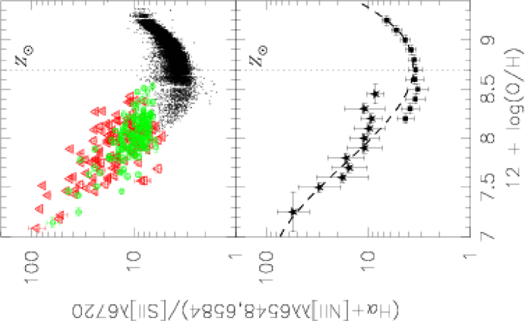
Figure 16: Same as Figure 15 but for the emission-line flux ratio of $F$(H$\alpha$+[Nii]$\lambda\lambda$6548,6584)/$F$([Sii]$\lambda$6720).

Another difficulty to measure the gas metallicities of high-$z$ galaxies is the faintness of targets, which sometimes prevents from measuring accurate emission-line fluxes. The use of low-resolution grating to improve the signal-to-noise ratio may yield to a blending of the H$\alpha$ and [Nii] emission lines, which results in poor determinations of the gas metallicity. Therefore It may be useful to investigate metallicity diagnostics which use the sum of $F$(H$\alpha$) and $F$([Nii]). In particular, we have examined the metallicity dependence of the flux ratio $F$(H$\alpha$+[Nii]$\lambda\lambda$6548,6584)/$F$([Sii]$\lambda$6720) in Figure 16. This group of lines can be measured even in low-resolution spectra and even in spectra covering a relatively narrow wavelength range, and therefore may be particularly useful in high-$z$ studies.There is a clear dependence of this flux ratio on the oxygen abundance, seen as a $\cup$-shaped distribution with a minimum at 12+log(O/H) $\sim$ 8.7 (i.e., $Z_{\rm gas}\sim Z_{\odot}$). The mean and the RMS of this flux ratio for each bin of oxygen abundance are given in Tables 7 and 8, and the coefficients of the fit are given in Tables 9 and 10. The observed distribution of this flux ratio is naturally expected, since the behavior of the nitrogen emission as a secondary element should dominate at the super-solar metallicity range, while $F$([Nii]) and $F$([Sii]) should become weak with respect to $F$(H$\alpha$) at the low-metallicities due to the decrease of the corresponding ions. Although this diagnostic like $R_{23}$ has two solutions when the ratio is below 10, this ratio seems useful for low-metallicity galaxies where it is larger than 10, in which case it is possible to state that the object belongs to the lower branch of the $\cup$-shaped distribution. This diagnostic is also useful when the [Sii] emission is not detected (this is frequently the case when high-$z$ faint galaxies are concerned). In this case, we can calculate a lower limit for this flux ratio, and we can derive accordingly an upper limit to the gas metallicity if the lower limit is larger than 10. Note that this diagnostic is essentially independent of dust reddening.

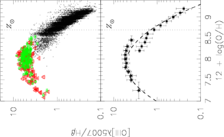
Figure 17: Same as Figure 15 but for the emission-line flux ratio of $F$([Oiii]$\lambda$5007)/$F$(H$\beta$).

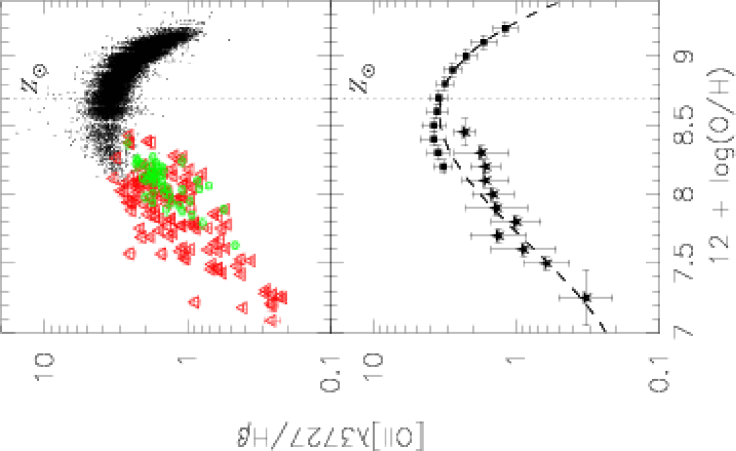
Figure 18: Same as Figure 15 but for the emission-line flux ratio of $F$([Oii]$\lambda$3727)/$F$(H$\beta$).

Finally, We have also investigated the flux ratios of $F$([Oiii]$\lambda$5007)/$F$(H$\beta$) and $F$([Oii]$\lambda$3727)/$F$(H$\beta$) (Figures 17 and 18). The empirical calibrations for these two flux ratios may be useful when either [Oii] or [Oiii] are not available, because out of the wavelength range or on a strong OH airglow emission line, or in a region of bad atmospheric transmission. The means and the RMSs of these two flux ratios for each bin of oxygen abundance are given in Tables 7 and 8, and the coefficients of the fit are given in Tables 9 and 10. As expected, both of the two flux ratios again show $\cap$-shaped distributions just similar to the $R_{23}$ parameter. The $F$([Oiii]$\lambda$5007)/$F$(H$\beta$) ratio is useful especially for high metallicity galaxies, because the targets should belong to the upper-branch of the distribution when $F$([Oiii]$\lambda$5007)/$F$(H$\beta$) $<$ 1 (although this might be wrong when extremely metal-poor galaxies [12+log(O/H) $<$ 7.0] are concerned). Note that this flux ratio is very sensitive to the oxygen abundance and the dispersion of the data is small at $F$([Oiii]$\lambda$5007)/$F$(H$\beta$) $<$ 1.

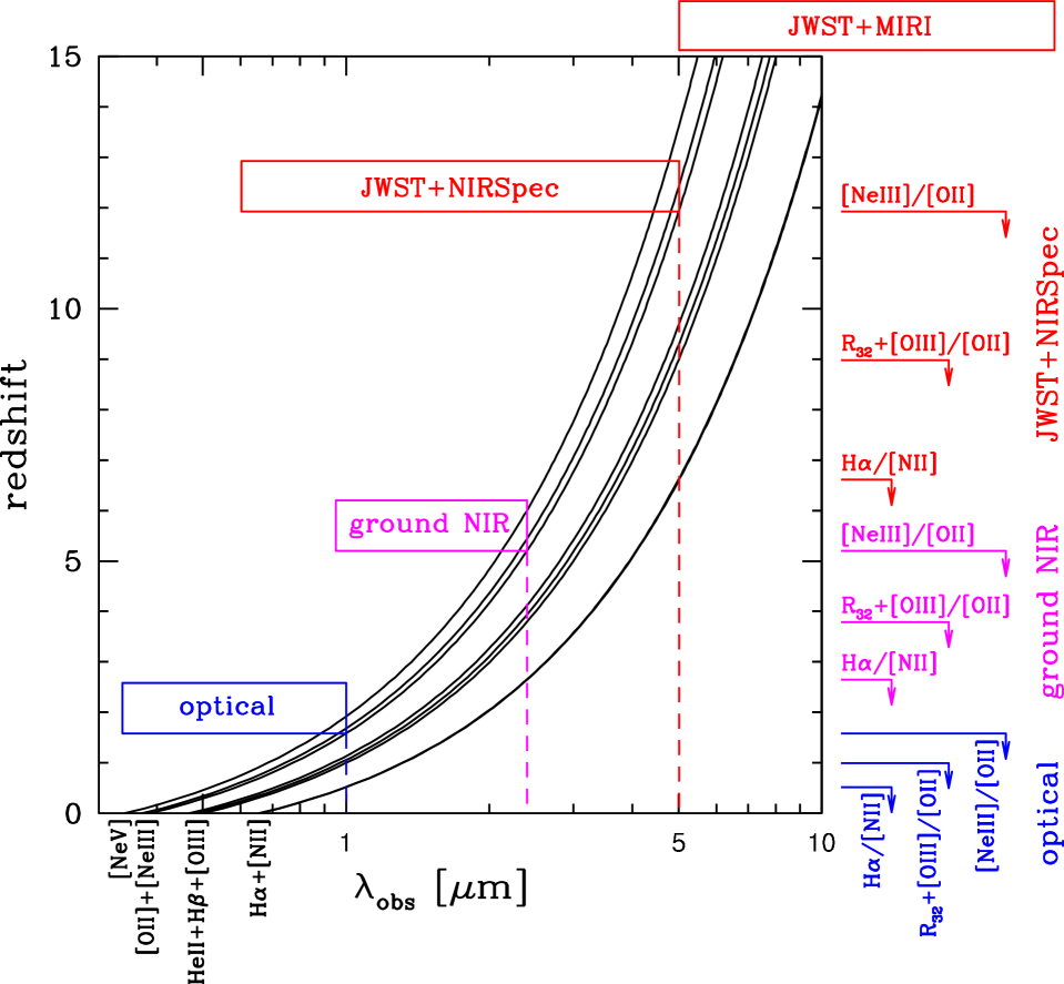
Figure 19: Schematic view of the availability of various metallicity diagnostics for each redshift. The black solid curves indicate the effect of redshift for some of the diagnostic lines discussed in this paper. The colored boxes indicate the wavelength coverages of optical spectrometers (blue), of ground-based near-IR spectrometers (magenta), and of NIRSpec/MIRI on board of JWST (red). The marks on the right of the diagram indicate the maximum redshift at which some of the metallicity diagnostics can be used with the various facilities.

Figure 19 summarizes the use of some of the metallicity diagnostics discussed in this paper as a function of redshift and for various observing facilities, and in particular optical spectrometers, ground-based near-IR spectrometers and NIRSpec on board of JWST. In principle (i.e., sensitivity permitting), MIRI on board of JWST will be able to observe the same diagnostics at even higher redshifts. Note that the ratio $F$([Neiii]$\lambda$3869)/$F$([Oii]$\lambda$3727) extends the diagnostic capability of any observing facility to significantly higher redshift.

5 Summary

We have combined two large spectroscopic datasets to derive empirical calibrations for gas metallicity diagnostics involving strong emission lines. The two datasets consist of about 50000 spectra from the SDSS DR4, which probe metallicities 12+log(O/H)$>$8.3 (sample C), and of 328 spectra of low metallicity galaxies with a measurement of the [Oiii]$\lambda$4363 line (sample A+B), which probe metallicities 12+log(O/H)$<$8.4. Together, these two samples provide the largest dataset of galaxies with known metallicity currently available, and spanning more than 2 dex in metallicity.

We have provided empirical calibrations both for metallicity diagnostics already proposed in the past and for new metallicity indicators proposed in this paper. We have given an analytical description for the metallicity dependence of the following diagnostics and line ratios: $R_{23}$, $F$([Nii]$\lambda$6584)/$F$(H$\alpha$), $F$([Oiii]$\lambda$5007)/$F$([Nii]$\lambda$6584), $F$([Nii]$\lambda$6584)/$F$([Oii]$\lambda$3727), $F$([Nii]$\lambda$6584)/ $F$([Sii]$\lambda$6720), $F$([Oiii]$\lambda$5007)/$F$([Oii]$\lambda$3727), and $F$([Neiii]$\lambda$3869)/$F$([Oii]$\lambda$3727). The calibrations are performed within the metallicity range 7.0 $\leq$ 12+log(O/H) $\leq$ 9.2. All of the investigated flux ratios show strong dependences on metallicity, at least in some metallicity ranges. We have shown that the monotonic metallicity dependence of the ratio $F$([Oiii]$\lambda$5007)/$F$([Oii]$\lambda$3727) can be used to break the degeneracy of the $R_{23}$ parameter when $F$([Nii]$\lambda$6584)/$F$(H$\alpha$) is not available. The $F$([Oiii]$\lambda$5007)/$F$([Oii]$\lambda$3727) ratio is particularly useful at high redshift, where H$\alpha$ and [Nii]$\lambda$6584 are shifted outside the observed band. Another promising metallicity tracer at high-$z$ is the ratio $F$([Neiii]$\lambda$3869)/$F$([Oii]$\lambda$3727), which is found to anti-correlate with metallicity. The $F$([Neiii]$\lambda$3869)/$F$([Oii]$\lambda$3727), ratio is particularly useful at high redshift, where most of the other diagnostic lines are shifted outside the observed band.

We have also investigated the observed relationships through a comparison with photoionization models. Some of the diagnostics investigated in this paper are strongly dependent on the ionization parameter $U$. The observed trends of these diagnostics highlight a clear, inverse relationship between ionization parameter and metallicity in galaxies. Such a strong $U$-$Z$ relationship is also required to explain the trend observed for the $R_{23}$ parameter. The $U$-$Z$ relationship is relatively tight and, indeed, we have found that at any given metallicity the ionization parameter has a small dispersion ($\sim$0.5 dex). The strong relationship between ionization parameter and metallicity in galaxies should warn about the use of simple models, which assume constant ionization parameter, to infer gas metallicities from line ratios.

Figure 1: Oxygen abundance of the galaxies in sample A, derived by Izotov et al. (2006b), as a function of redshift.

Figure 2: Emission-line flux ratios of [Sii]$\lambda$6717/[Sii]$\lambda$6731 for the compiled low-metallicity galaxies, as a function of the oxygen abundance derived by us (see §§2.1.2). The upper horizontal dotted line denotes the theoretical low-density limit of this flux ratio and the lower dotted line denotes the high-density limit.

Figure 3: Oxygen abundances of the compiled low-metallicity galaxies re-calculated by us (see §§2.1.2) are plotted as a function of the oxygen abundances given in the original references. Dotted line is not the best-fit line but a reference line for the case when the two quantities are the same.

Figure 4: Frequency distribution of the redshift of the SDSS DR4 galaxies after our sample selection (sample C) described in §§2.2. Galaxies at $z<0.028$ are not included (see text).

Figure 5: Frequency distribution of the oxygen abundance of galaxies in sample C.

Figure 8: Same as Figure 6 but means and the RMS values are shown in each bin of oxygen abundance, instead of individual data. Filled squares and filled stars denote the mean flux ratios for galaxies in sample C and those for galaxies in sample A+B, respectively. The errorbar denotes the RMS. The dashed line denotes the best-fit polynomial function, as described in the text. Dashed lines denote the solar metallicity [12+log(O/H) = 8.69].

Figure 9: Same as Figure 8 but for the emission-line flux ratios of $F$([Nii]$\lambda$6584)/$F$([Oii]$\lambda$3727), $F$([Nii]$\lambda$6584)/$F$([Sii]$\lambda$6720), and $F$([Oiii]$\lambda$5007)/$F$([Oii]$\lambda$3727).

Figure 13: The averaged flux ratios and the best-fit polynomial functions of the metallicity dependence of $R_{23}$, $F$([Nii]$\lambda$6584)/$F$(H$\alpha$) and $F$([Oiii]$\lambda$5007)/$F$([Nii]$\lambda$6584) (dashed line) are compared with the predictions of photoionization models (solid lines: Kewley & Dopita 2002; Kobulnicky & Kewley 2004). The lines with a digit 1, 2, 3, 4, 5, 6, and 7 denote the model predictions with the ionization parameter of log $U$ = –3.8, –3.5, –3.2, –2.9, –2.6, –2.3, and –2.0, respectively. Dotted line denotes the solar metallicity [12+log(O/H) = 8.69].

Figure 14: Same as Figure 13 but for the emission-line flux ratios of $F$([Nii]$\lambda$6584)/$F$([Oii]$\lambda$3727), $F$([Nii]$\lambda$6584)/$F$([Sii]$\lambda$6720), and $F$([Oiii]$\lambda$5007)/$F$([Oii]$\lambda$3727).

Table 1: Re-calculated properties of the compiled low-metallicity galaxies

Object	$R_{23}$	$n_{\rm H}$(S+)a	$t$(O2+)b	12 + log(O/H)	Ref.c
HS 0029+1748	8.624 $\pm$ 0.168	$70^{+47}_{-42}$	$1.286\pm 0.016$	8.046 $\pm$ 0.016	I04b
HS 0111+2115	9.142 $\pm$ 0.179	$<22$	$1.108^{+0.063}_{-0.066}$	8.290 $\pm$ 0.076	I04b
HS 0122+0743	6.669 $\pm$ 0.127	$42^{+59}_{-42}$	$1.777\pm 0.025$	7.597 $\pm$ 0.014	I04b
HS 0128+2832	10.272 $\pm$ 0.197	$104^{+40}_{-37}$	$1.256\pm 0.011$	8.147 $\pm$ 0.013	I04b
HS 0134+3415	10.485 $\pm$ 0.204	$200^{+76}_{-68}$	$1.639\pm 0.019$	7.858 $\pm$ 0.014	I04b
HS 0735+3512	9.640 $\pm$ 0.163	$75^{+39}_{-36}$	$1.205\pm 0.015$	8.193 $\pm$ 0.014	I04b
HS 0811+4913	9.861 $\pm$ 0.184	$44^{+51}_{-44}$	$1.449\pm 0.016$	7.968 $\pm$ 0.013	I04b
HS 0837+4717	8.061 $\pm$ 0.153	$373^{+117}_{-101}$	$1.954\pm 0.026$	7.587 $\pm$ 0.013	I04b
HS 0924+3821	8.617 $\pm$ 0.152	$16^{+44}_{-16}$	$1.256\pm 0.021$	8.089 $\pm$ 0.018	I04b
HS 1028+3843	10.464 $\pm$ 0.206	$492^{+138}_{-117}$	$1.582\pm 0.017$	7.891 $\pm$ 0.014	I04b
HS 1213+3636A	7.353 $\pm$ 0.112	$35^{+35}_{-32}$	$1.074^{+0.026}_{-0.027}$	8.263 $\pm$ 0.033	I04b
HS 1214+3801	9.095 $\pm$ 0.162	$20^{+37}_{-20}$	$1.339\pm 0.013$	8.026 $\pm$ 0.012	I04b
HS 1311+3628	8.570 $\pm$ 0.146	$95^{+38}_{-35}$	$1.141\pm 0.013$	8.199 $\pm$ 0.015	I04b
HS 2236+1344	6.975 $\pm$ 0.135	$86^{+131}_{-86}$	$2.123\pm 0.032$	7.464 $\pm$ 0.013	I04b
HS 2359+1659	9.608 $\pm$ 0.125	$<10$	$1.189^{+0.016}_{-0.017}$	8.179 $\pm$ 0.017	I04b
IC 0010 1	6.757 $\pm$ 0.400	(10)d	$1.015^{+0.077}_{-0.085}$	8.301 $\pm$ 0.096	L03b
IC 0010 2	6.607 $\pm$ 0.369	(10)d	$0.984^{+0.077}_{-0.086}$	8.335 $\pm$ 0.097	L03b
IC 0010 3	7.658 $\pm$ 0.624	(10)d	$1.236^{+0.155}_{-0.169}$	8.083 $\pm$ 0.128	L03b
IC 1613	7.641 $\pm$ 0.822	$<167$	$1.796^{+0.161}_{-0.158}$	7.643 $\pm$ 0.085	L03a
IC 5152	5.852 $\pm$ 0.509	$21^{+275}_{-21}$	$1.240^{+0.166}_{-0.183}$	7.955 $\pm$ 0.135	L03a
KISSB 0023	5.251 $\pm$ 0.238	$<172$	$1.833^{+0.094}_{-0.093}$	7.570 $\pm$ 0.030	M04
KISSB 0061	7.348 $\pm$ 0.239	$<10$	$1.565^{+0.037}_{-0.038}$	7.772 $\pm$ 0.024	L04
KISSB 0086	8.177 $\pm$ 0.242	$<10$	$1.241\pm 0.028$	8.088 $\pm$ 0.025	L04
KISSB 0171	8.276 $\pm$ 0.247	$<35$	$1.189\pm 0.020$	8.121 $\pm$ 0.022	L04
KISSB 0175	9.346 $\pm$ 0.295	$166^{+139}_{-110}$	$1.344\pm 0.024$	8.041 $\pm$ 0.021	L04
KISSR 0049	7.786 $\pm$ 0.398	$95^{+291}_{-95}$	$1.305^{+0.083}_{-0.086}$	8.028 $\pm$ 0.059	M04
KISSR 0073	7.424 $\pm$ 0.382	$13^{+194}_{-13}$	$1.366^{+0.056}_{-0.057}$	7.943 $\pm$ 0.042	L04
KISSR 0085	5.316 $\pm$ 0.222	$833^{+727}_{-412}$	$1.775^{+0.104}_{-0.103}$	7.532 $\pm$ 0.043	M04
KISSR 0087	7.827 $\pm$ 0.247	$71^{+111}_{-71}$	$0.996\pm 0.023$	8.386 $\pm$ 0.030	L04
KISSR 0116	7.826 $\pm$ 0.241	$<90$	$1.205^{+0.021}_{-0.022}$	8.107 $\pm$ 0.022	L04
KISSR 0286	7.710 $\pm$ 0.235	$29^{+103}_{-29}$	$1.103\pm 0.022$	8.216 $\pm$ 0.028	L04
KISSR 0310	9.501 $\pm$ 0.551	$26^{+198}_{-26}$	$1.528\pm 0.050$	7.892 $\pm$ 0.039	L04
KISSR 0311	8.935 $\pm$ 0.468	$32^{+192}_{-32}$	$1.387^{+0.045}_{-0.046}$	7.994 $\pm$ 0.036	L04
KISSR 0396	8.023 $\pm$ 0.238	$27^{+69}_{-27}$	$1.406^{+0.046}_{-0.047}$	7.938 $\pm$ 0.029	M04
KISSR 0666	8.630 $\pm$ 0.397	$<10$	$2.153^{+0.092}_{-0.090}$	7.528 $\pm$ 0.038	M04
KISSR 0675	8.773 $\pm$ 0.583	$1138^{+2735}_{-763}$	$1.507^{+0.112}_{-0.114}$	7.890 $\pm$ 0.071	M04
KISSR 0814	8.620 $\pm$ 0.276	$79^{+132}_{-79}$	$1.373\pm 0.026$	7.983 $\pm$ 0.022	L04
KISSR 1013	7.271 $\pm$ 0.295	$474^{+346}_{-239}$	$1.781^{+0.105}_{-0.104}$	7.690 $\pm$ 0.038	M04
KISSR 1194	8.836 $\pm$ 0.356	$51^{+240}_{-51}$	$1.458^{+0.041}_{-0.042}$	7.930 $\pm$ 0.029	M04
KISSR 1490	6.676 $\pm$ 0.308	$<381$	$1.903^{+0.110}_{-0.109}$	7.568 $\pm$ 0.040	M04
KISSR 1778	6.628 $\pm$ 0.325	$69^{+383}_{-69}$	$1.305^{+0.091}_{-0.094}$	7.955 $\pm$ 0.064	M04
KISSR 1845	9.440 $\pm$ 0.381	$50^{+240}_{-50}$	$1.325\pm 0.033$	8.069 $\pm$ 0.028	M04
Mrk 0005	7.192 $\pm$ 0.106	$13^{+54}_{-13}$	$1.220^{+0.051}_{-0.052}$	8.058 $\pm$ 0.041	I98
Mrk 0022	8.726 $\pm$ 0.101	$71^{+55}_{-49}$	$1.349^{+0.020}_{-0.021}$	8.002 $\pm$ 0.015	I94
Mrk 0035	7.892 $\pm$ 0.121	$189^{+36}_{-34}$	$1.021^{+0.012}_{-0.013}$	8.368 $\pm$ 0.015	I04b
Mrk 0036	7.708 $\pm$ 0.092	$<102$	$1.524\pm 0.037$	7.816 $\pm$ 0.021	I98
Mrk 0067	9.309 $\pm$ 0.176	$<10$	$1.320\pm 0.024$	8.059 $\pm$ 0.019	I04b
Mrk 0116	2.937 $\pm$ 0.017	$86^{+112}_{-86}$	$1.927\pm 0.038$	7.178 $\pm$ 0.014	I97
Mrk 0116 1	2.935 $\pm$ 0.043	$<1369$	$2.133^{+0.064}_{-0.063}$	7.084 $\pm$ 0.023	P92
Mrk 0116 2	3.009 $\pm$ 0.071	$68^{+722}_{-68}$	$1.979^{+0.092}_{-0.090}$	7.217 $\pm$ 0.027	P92
Mrk 0162	8.180 $\pm$ 0.083	$<10$	$1.194^{+0.043}_{-0.044}$	8.116 $\pm$ 0.034	I98
Mrk 0178	8.517 $\pm$ 0.245	$122^{+234}_{-122}$	$1.588\pm 0.104$	7.816 $\pm$ 0.057	G00
Mrk 0193	8.906 $\pm$ 0.101	$172^{+93}_{-81}$	$1.639\pm 0.019$	7.795 $\pm$ 0.011	I94
Mrk 0209	8.075 $\pm$ 0.018	$46^{+45}_{-42}$	$1.630\pm 0.007$	7.755 $\pm$ 0.004	I97
Mrk 0450 1	8.514 $\pm$ 0.144	$132^{+39}_{-36}$	$1.173\pm 0.013$	8.154 $\pm$ 0.014	I04b
Mrk 0450 2	8.661 $\pm$ 0.166	$<21$	$1.251^{+0.028}_{-0.029}$	8.094 $\pm$ 0.024	I04b
Mrk 0475	8.392 $\pm$ 0.111	$<45$	$1.411\pm 0.028$	7.933 $\pm$ 0.019	I94

Table 1: Re-calculated properties of the compiled low-metallicity galaxies (continued)

Object	$R_{23}$	$n_{\rm H}$(S+)a	$t$(O2+)b	12 + log(O/H)	Ref.c
Mrk 0487	8.413 $\pm$ 0.157	$63^{+92}_{-63}$	$1.266^{+0.057}_{-0.058}$	8.076 $\pm$ 0.043	I97
Mrk 0600	8.578 $\pm$ 0.101	$58^{+41}_{-38}$	$1.579\pm 0.020$	7.824 $\pm$ 0.012	I98
Mrk 0724	8.618 $\pm$ 0.149	$19^{+37}_{-19}$	$1.296^{+0.014}_{-0.015}$	8.045 $\pm$ 0.013	I04b
Mrk 0750	8.357 $\pm$ 0.079	$<10$	$1.205^{+0.023}_{-0.024}$	8.128 $\pm$ 0.021	I98
Mrk 0930	7.905 $\pm$ 0.084	$56^{+40}_{-36}$	$1.236^{+0.037}_{-0.038}$	8.084 $\pm$ 0.029	I98
Mrk 1063	6.183 $\pm$ 0.106	$96^{+43}_{-39}$	$1.027^{+0.058}_{-0.062}$	8.260 $\pm$ 0.069	I04b
Mrk 1089	5.554 $\pm$ 0.057	$92^{+43}_{-39}$	$1.108^{+0.069}_{-0.074}$	8.090 $\pm$ 0.070	I98
Mrk 1236	9.550 $\pm$ 0.170	$47^{+35}_{-33}$	$1.225\pm 0.012$	8.157 $\pm$ 0.013	I04b
Mrk 1271	9.680 $\pm$ 0.074	$52^{+51}_{-47}$	$1.411\pm 0.018$	7.996 $\pm$ 0.012	I98
Mrk 1315	9.104 $\pm$ 0.164	$11^{+30}_{-11}$	$1.103\pm 0.009$	8.270 $\pm$ 0.013	I04b
Mrk 1328	6.981 $\pm$ 0.165	$25^{+83}_{-25}$	$0.937^{+0.099}_{-0.119}$	8.457 $\pm$ 0.106	V03
Mrk 1329	8.539 $\pm$ 0.150	$18^{+31}_{-18}$	$1.080\pm 0.009$	8.278 $\pm$ 0.013	I04b
Mrk 1409	8.754 $\pm$ 0.138	$599^{+124}_{-106}$	$1.362^{+0.066}_{-0.067}$	8.025 $\pm$ 0.040	I97
Mrk 1416	8.098 $\pm$ 0.065	$<10$	$1.514\pm 0.031$	7.854 $\pm$ 0.016	I97
Mrk 1434	7.640 $\pm$ 0.049	$<10$	$1.551\pm 0.015$	7.786 $\pm$ 0.009	I97
Mrk 1450	7.669 $\pm$ 0.052	$<43$	$1.330\pm 0.016$	7.963 $\pm$ 0.012	I94
Mrk 1486	8.140 $\pm$ 0.059	$27^{+40}_{-27}$	$1.468\pm 0.022$	7.884 $\pm$ 0.013	I97
NGC 2363 A	9.358 $\pm$ 0.020	$85^{+58}_{-53}$	$1.584\pm 0.006$	7.843 $\pm$ 0.004	I97
NGC 2363 B	7.286 $\pm$ 0.074	$14^{+70}_{-14}$	$1.496^{+0.033}_{-0.034}$	7.818 $\pm$ 0.019	I97
NGC 3109	6.221 $\pm$ 0.437	(10)d	$1.463^{+0.262}_{-0.277}$	7.792 $\pm$ 0.138	L03b
NGC 4214 A6	6.898 $\pm$ 0.162	$33^{+93}_{-33}$	$1.051^{+0.047}_{-0.050}$	8.280 $\pm$ 0.062	K96
NGC 4214 C6	7.913 $\pm$ 0.176	$74^{+98}_{-74}$	$0.983^{+0.024}_{-0.025}$	8.426 $\pm$ 0.029	K96
NGC 4861	8.801 $\pm$ 0.020	$74^{+27}_{-26}$	$1.363\pm 0.006$	7.987 $\pm$ 0.005	I97
PGC 18096	10.671 $\pm$ 0.124	$195^{+64}_{-57}$	$1.339\pm 0.021$	8.086 $\pm$ 0.017	G00
PGC 27864 1	8.410 $\pm$ 0.151	$116^{+47}_{-43}$	$1.648\pm 0.018$	7.771 $\pm$ 0.012	I04b
PGC 27864 2	7.616 $\pm$ 0.135	$<10$	$1.657\pm 0.027$	7.738 $\pm$ 0.014	I04b
PGC 37727	8.082 $\pm$ 0.129	$57^{+39}_{-36}$	$1.256^{+0.029}_{-0.030}$	8.079 $\pm$ 0.022	I04b
PGC 39188	7.325 $\pm$ 0.091	$1088^{+120}_{-107}$	$1.014^{+0.026}_{-0.027}$	8.375 $\pm$ 0.030	V03
PGC 39402	7.368 $\pm$ 0.146	$261^{+117}_{-100}$	$2.002\pm 0.028$	7.518 $\pm$ 0.014	I04
PGC 39845	5.990 $\pm$ 0.181	$140^{+305}_{-140}$	$1.689\pm 0.146$	7.653 $\pm$ 0.051	V03
PGC 40521	5.549 $\pm$ 0.350	$57^{+326}_{-57}$	$1.330^{+0.221}_{-0.241}$	7.864 $\pm$ 0.145	V03
PGC 40582 1	5.814 $\pm$ 0.113	$108^{+74}_{-66}$	$1.880\pm 0.031$	7.480 $\pm$ 0.015	I04a
PGC 40582 2	5.033 $\pm$ 0.103	$<10$	$1.829^{+0.057}_{-0.056}$	7.456 $\pm$ 0.025	I04a
PGC 40582 3	4.901 $\pm$ 0.187	$<62$	$1.908^{+0.342}_{-0.327}$	7.410 $\pm$ 0.125	I04a
PGC 40582 4	5.670 $\pm$ 0.131	(10)d	$1.918^{+0.078}_{-0.077}$	7.458 $\pm$ 0.032	I04a
PGC 40604	7.671 $\pm$ 0.266	$<127$	$1.266^{+0.162}_{-0.176}$	8.058 $\pm$ 0.120	V03
PGC 40604 a	6.668 $\pm$ 0.279	$155^{+273}_{-155}$	$1.275^{+0.157}_{-0.170}$	7.972 $\pm$ 0.118	V03
PGC 41360	7.255 $\pm$ 0.187	$39^{+107}_{-39}$	$1.542\pm 0.047$	7.775 $\pm$ 0.029	V03
PGC 42160	5.418 $\pm$ 0.238	$<123$	$1.486^{+0.229}_{-0.238}$	7.744 $\pm$ 0.104	V03
PGC 49050	7.773 $\pm$ 0.538	$<157$	$1.103^{+0.127}_{-0.144}$	8.250 $\pm$ 0.194	L03a
SBS 0335–052	4.343 $\pm$ 0.041	$275^{+225}_{-172}$	$2.040\pm 0.036$	7.280 $\pm$ 0.014	I98
SBS 0335–052 E3	4.588 $\pm$ 0.090	(10)d	$2.027\pm 0.029$	7.306 $\pm$ 0.014	P06
SBS 0335–052 E4-5	4.443 $\pm$ 0.093	(10)d	$2.128^{+0.041}_{-0.040}$	7.248 $\pm$ 0.017	P06
SBS 0335–052 E7	3.457 $\pm$ 0.074	(10)d	$1.974^{+0.063}_{-0.062}$	7.209 $\pm$ 0.027	P06
SBS 0335–052 E-NW	3.446 $\pm$ 0.097	(10)d	$2.001^{+0.125}_{-0.122}$	7.194 $\pm$ 0.049	P06
SBS 0335–052 E-SE	4.087 $\pm$ 0.085	(10)d	$1.979\pm 0.053$	7.275 $\pm$ 0.023	P06
SBS 0335–052 W	2.550 $\pm$ 0.072	(10)d	$1.974^{+0.260}_{-0.249}$	7.133 $\pm$ 0.073	P06
SBS 0749+568	8.144 $\pm$ 0.227	$<10$	$1.528\pm 0.081$	7.843 $\pm$ 0.045	I97
SBS 0749+582	11.727 $\pm$ 0.272	$117^{+155}_{-117}$	$1.334\pm 0.034$	8.135 $\pm$ 0.028	I97
SBS 0907+543	10.014 $\pm$ 0.241	$118^{+277}_{-118}$	$1.444\pm 0.043$	7.974 $\pm$ 0.031	I97
SBS 0926+606	8.117 $\pm$ 0.059	$188^{+48}_{-45}$	$1.434\pm 0.023$	7.911 $\pm$ 0.014	I97
SBS 0940+544	5.853 $\pm$ 0.081	$188^{+187}_{-146}$	$2.016\pm 0.038$	7.430 $\pm$ 0.015	I97
SBS 0943+561	9.024 $\pm$ 0.424	$271^{+630}_{-271}$	$1.758^{+0.130}_{-0.129}$	7.749 $\pm$ 0.060	I97
SBS 0948+532	8.841 $\pm$ 0.144	$73^{+85}_{-73}$	$1.339\pm 0.027$	8.014 $\pm$ 0.021	I94
SBS 1054+365	8.959 $\pm$ 0.090	$<27$	$1.383\pm 0.019$	7.978 $\pm$ 0.014	I97
SBS 1116+583B	7.014 $\pm$ 0.249	$593^{+617}_{-351}$	$1.670\pm 0.089$	7.673 $\pm$ 0.049	I97
SBS 1128+573	8.570 $\pm$ 0.212	$211^{+339}_{-211}$	$1.689\pm 0.062$	7.751 $\pm$ 0.033	I97

Table 1: Re-calculated properties of the compiled low-metallicity galaxies (continued)

Object	$R_{23}$	$n_{\rm H}$(S+)a	$t$(O2+)b	12 + log(O/H)	Ref.c
SBS 1129+576a	3.851 $\pm$ 0.111	$<248$	$1.899^{+0.271}_{-0.262}$	7.369 $\pm$ 0.069	G03a
SBS 1129+576b	5.804 $\pm$ 0.247	$<287$	$2.094^{+0.291}_{-0.275}$	7.475 $\pm$ 0.064	G03a
SBS 1159+545	5.620 $\pm$ 0.051	$57^{+54}_{-50}$	$1.852\pm 0.020$	7.491 $\pm$ 0.009	I98
SBS 1205+557	7.067 $\pm$ 0.103	$<76$	$1.607\pm 0.067$	7.752 $\pm$ 0.029	I97
SBS 1211+540	6.814 $\pm$ 0.073	$168^{+124}_{-103}$	$1.699\pm 0.024$	7.644 $\pm$ 0.013	I94
SBS 1222+614	9.071 $\pm$ 0.050	$22^{+28}_{-22}$	$1.425\pm 0.012$	7.951 $\pm$ 0.009	I97
SBS 1249+493	7.359 $\pm$ 0.087	$<10$	$1.648\pm 0.024$	7.721 $\pm$ 0.012	I98
SBS 1319+579 A	9.913 $\pm$ 0.066	$145^{+26}_{-25}$	$1.310^{+0.011}_{-0.012}$	8.084 $\pm$ 0.010	I97
SBS 1319+579 B	6.797 $\pm$ 0.189	$40^{+113}_{-40}$	$1.359^{+0.165}_{-0.175}$	7.911 $\pm$ 0.102	I97
SBS 1319+579 C	7.054 $\pm$ 0.061	$20^{+33}_{-20}$	$1.136^{+0.035}_{-0.036}$	8.136 $\pm$ 0.032	I97
SBS 1331+493	8.129 $\pm$ 0.110	$164^{+93}_{-81}$	$1.602\pm 0.027$	7.780 $\pm$ 0.016	I94
SBS 1331+493S	6.308 $\pm$ 0.138	$<79$	$1.353^{+0.086}_{-0.088}$	7.885 $\pm$ 0.056	T95
SBS 1415+437	5.677 $\pm$ 0.025	$65^{+31}_{-30}$	$1.703\pm 0.011$	7.586 $\pm$ 0.005	I98
SBS 1415+437e1	5.649 $\pm$ 0.025	$48^{+31}_{-30}$	$1.657\pm 0.010$	7.601 $\pm$ 0.005	G03c
SBS 1415+437e2	5.290 $\pm$ 0.079	$79^{+114}_{-79}$	$1.597\pm 0.056$	7.614 $\pm$ 0.028	G03c
SBS 1420+544	9.683 $\pm$ 0.070	$<10$	$1.764\pm 0.011$	7.752 $\pm$ 0.006	I98
SBS 1533+469	8.690 $\pm$ 0.226	$46^{+106}_{-46}$	$1.383^{+0.054}_{-0.055}$	7.984 $\pm$ 0.035	T95
SBS 1533+574 A	7.507 $\pm$ 0.081	$30^{+48}_{-30}$	$1.444\pm 0.057$	7.883 $\pm$ 0.031	I97
SBS 1533+574 B	9.107 $\pm$ 0.083	$<23$	$1.246\pm 0.029$	8.124 $\pm$ 0.023	I97
SDSS J0113+0052	3.402 $\pm$ 0.211	(10)d	$2.317^{+0.325}_{-0.301}$	7.163 $\pm$ 0.076	I06
SDSS J0519+0007	6.176 $\pm$ 0.122	$373^{+308}_{-220}$	$2.078\pm 0.036$	7.420 $\pm$ 0.015	I04b
SDSS J2104–0035 N	4.044 $\pm$ 0.093	(10)d	$2.008\pm 0.066$	7.257 $\pm$ 0.028	I06
UGC 4305 5	5.383 $\pm$ 0.354	(10)d	$1.607^{+0.147}_{-0.148}$	7.647 $\pm$ 0.064	L03b
UGC 4305 7	5.150 $\pm$ 0.280	(10)d	$1.354^{+0.208}_{-0.224}$	7.806 $\pm$ 0.129	L03b
UGC 4305 8	5.010 $\pm$ 0.306	(10)d	$1.514^{+0.188}_{-0.193}$	7.677 $\pm$ 0.086	L03b
UGC 4305 9	5.371 $\pm$ 0.379	(10)d	$1.486^{+0.124}_{-0.126}$	7.699 $\pm$ 0.072	L03b
UGC 4483	4.795 $\pm$ 0.052	$72^{+93}_{-72}$	$1.657\pm 0.026$	7.540 $\pm$ 0.012	I94
UGC 6456	5.918 $\pm$ 0.062	$29^{+52}_{-29}$	$1.547\pm 0.022$	7.696 $\pm$ 0.012	I97
UGC 6456 1	4.395 $\pm$ 0.399	(10)d	$2.089^{+0.476}_{-0.436}$	7.355 $\pm$ 0.108	L03b
UGC 6456 2	5.180 $\pm$ 0.372	(10)d	$1.768^{+0.191}_{-0.188}$	7.519 $\pm$ 0.077	L03b
UGC 9128	4.178 $\pm$ 0.166	$198\pm 16$	$1.320^{+0.121}_{-0.127}$	7.745 $\pm$ 0.080	L03b
UGC 9497 c	7.138 $\pm$ 0.101	$<77$	$1.796\pm 0.030$	7.608 $\pm$ 0.015	G03b
UGC 9497 e	4.451 $\pm$ 0.307	$<453$	$1.657^{+0.435}_{-0.440}$	7.524 $\pm$ 0.172	G03b
UM 133	6.784 $\pm$ 0.112	$<26$	$1.676\pm 0.032$	7.692 $\pm$ 0.014	I04b
UM 238	10.786 $\pm$ 0.219	$288^{+69}_{-61}$	$1.250\pm 0.016$	8.177 $\pm$ 0.017	I04b
UM 311	7.075 $\pm$ 0.077	$75^{+40}_{-36}$	$0.977^{+0.037}_{-0.039}$	8.374 $\pm$ 0.044	I98
UM 396	9.391 $\pm$ 0.177	$37^{+44}_{-37}$	$1.136\pm 0.016$	8.238 $\pm$ 0.019	I04b
UM 420	7.814 $\pm$ 0.182	$<79$	$1.387^{+0.081}_{-0.083}$	7.941 $\pm$ 0.049	I98
UM 422	10.519 $\pm$ 0.200	$<57$	$1.296\pm 0.014$	8.121 $\pm$ 0.014	I04b
UM 439	11.735 $\pm$ 0.226	$177^{+59}_{-53}$	$1.411\pm 0.015$	8.069 $\pm$ 0.013	I04b
UM 448	6.225 $\pm$ 0.067	$138^{+35}_{-33}$	$1.220^{+0.059}_{-0.061}$	8.018 $\pm$ 0.047	I98
UM 461	8.518 $\pm$ 0.200	$203^{+284}_{-194}$	$1.615\pm 0.042$	7.782 $\pm$ 0.027	I98
UM 462 SW	8.283 $\pm$ 0.052	$<10$	$1.378\pm 0.015$	7.960 $\pm$ 0.010	I98

• Gas density of the S⁺ regions in units of cm^-3.

• Gas temperature of the O²⁺ regions in units of $10^{4}$K.

• References. — G00: Guseva et al. (2000), G03a: Guseva et al. (2003a), G03b: Guseva et al. (2003b), G03c: Guseva et al. (2003c), I94: Izotov et al. (1994), I97: Izotov et al. (1997), I98: Izotov & Thuan (1998), I04a: Izotov et al. (2004), I04b: Izotov & Thuan (2004), I06: Izotov et al. (2006a), K96: Kobulnicky & Skillman (1996), L03a: Lee et al. (2003a), L03b: Lee et al. (2003b), L04: Lee et al. (2004), M04: Melbourne et al. (2004), P92: Pagel et al. (1992), P06: Papaderos et al. (2006), T95: Thuan et al. (1995), V03: Vílchez & Iglesias-Páramo (2003).

• Flux ratio of [Sii] is not given in literature. We adopt $n_{\rm H}$(S⁺) = 10 cm^-3 to calculate the oxygen abundance for these objects.

Table 2: Statistical properties of the samples

Sample	$N_{\rm obj}$	Median of 12+log(O/H)	Mean of 12+log(O/H)	RMS of 12+log(O/H)
Sample A	139	8.010	8.003	0.233
Sample B	120	7.936	7.858	0.303
Sample C	48497	9.016	8.976	0.166
Sample A+B	259	7.980	7.936	0.277

Table 3: Means and RMSs of emission-line flux ratios of the galaxies in the sample A+B^a

Oxygen Abundance	log$R_{23}$	log$\frac{F([{\rm NII}]\lambda 6584)}{F({\rm H}\alpha)}$	log$\frac{F([{\rm OIII}]\lambda 5007)}{F([{\rm NII}]\lambda 6584)}$	log$\frac{F([{\rm NII}]\lambda 6584)}{F([{\rm OII}]\lambda 3727)}$	log$\frac{F([{\rm NII}]\lambda 6584)}{F([{\rm SII}]\lambda 6720)}$	log$\frac{F([{\rm OIII}]\lambda 5007)}{F([{\rm OII}]\lambda 3727)}$
$7.05\!\leq\!12\!+\!{\rm log(O/H)}\!<\!7.45$	0.601	–2.452	2.415	–1.657	–0.668	0.920
	(0.108)	(0.238)	(0.196)	(0.269)	(0.178)	(0.247)
$7.45\!\leq\!12\!+\!{\rm log(O/H)}\!<\!7.55$	0.780	–2.122	2.278	–1.477	–0.606	0.814
	(0.084)	(0.272)	(0.343)	(0.120)	(0.111)	(0.262)
$7.55\!\leq\!12\!+\!{\rm log(O/H)}\!<\!7.65$	0.809	–1.844	2.006	–1.376	–0.566	0.652
	(0.068)	(0.195)	(0.274)	(0.183)	(0.197)	(0.356)
$7.65\!\leq\!12\!+\!{\rm log(O/H)}\!<\!7.75$	0.843	–1.846	2.050	–1.431	–0.599	0.492
	(0.039)	(0.247)	(0.290)	(0.176)	(0.075)	(0.233)
$7.75\!\leq\!12\!+\!{\rm log(O/H)}\!<\!7.85$	0.909	–1.887	2.162	–1.458	–0.621	0.719
	(0.039)	(0.205)	(0.260)	(0.129)	(0.112)	(0.233)
$7.85\!\leq\!12\!+\!{\rm log(O/H)}\!<\!7.95$	0.928	–1.624	1.884	–1.281	–0.531	0.579
	(0.045)	(0.197)	(0.262)	(0.167)	(0.140)	(0.307)
$7.95\!\leq\!12\!+\!{\rm log(O/H)}\!<\!8.05$	0.941	–1.578	1.858	–1.262	–0.484	0.571
	(0.042)	(0.213)	(0.280)	(0.179)	(0.118)	(0.218)
$8.05\!\leq\!12\!+\!{\rm log(O/H)}\!<\!8.15$	0.944	–1.481	1.759	–1.227	–0.450	0.511
	(0.053)	(0.177)	(0.255)	(0.149)	(0.109)	(0.247)
$8.15\!\leq\!12\!+\!{\rm log(O/H)}\!<\!8.25$	0.938	–1.375	1.631	–1.119	–0.348	0.514
	(0.044)	(0.142)	(0.185)	(0.114)	(0.120)	(0.168)
$8.25\!\leq\!12\!+\!{\rm log(O/H)}\!<\!8.35$	0.917	–1.415	1.641	–1.201	–0.333	0.436
	(0.036)	(0.196)	(0.260)	(0.101)	(0.064)	(0.288)
$8.35\!\leq\!12\!+\!{\rm log(O/H)}\!<\!8.55$	0.892	–1.124	1.259	–1.084	–0.173	0.258
	(0.034)	(0.176)	(0.221)	(0.109)	(0.122)	(0.087)

• Mean and RMS of each emission-line flux ratio are given in the upper and lower rows. RMSs are given in parenthesis.

Table 4: Means and RMSs of emission-line flux ratios of the galaxies in sample C^a

Oxygen Abundance	log$R_{23}$	log$\frac{F([{\rm NII}]\lambda 6584)}{F({\rm H}\alpha)}$	log$\frac{F([{\rm OIII}]\lambda 5007)}{F([{\rm NII}]\lambda 6584)}$	log$\frac{F([{\rm NII}]\lambda 6584)}{F([{\rm OII}]\lambda 3727)}$	log$\frac{F([{\rm NII}]\lambda 6584)}{F([{\rm SII}]\lambda 6720)}$	log$\frac{F([{\rm OIII}]\lambda 5007)}{F([{\rm OII}]\lambda 3727)}$
$8.15\!\leq\!12\!+\!{\rm log(O/H)}\!<\!8.25$	0.835	–1.138	1.102	–1.196	–0.532	–0.089
	(0.043)	(0.081)	(0.171)	(0.077)	(0.042)	(0.140)
$8.25\!\leq\!12\!+\!{\rm log(O/H)}\!<\!8.35$	0.825	–1.031	0.936	–1.113	–0.480	–0.191
	(0.053)	(0.077)	(0.187)	(0.082)	(0.038)	(0.170)
$8.35\!\leq\!12\!+\!{\rm log(O/H)}\!<\!8.45$	0.817	–0.934	0.768	–1.056	–0.444	–0.283
	(0.060)	(0.088)	(0.199)	(0.084)	(0.033)	(0.174)
$8.45\!\leq\!12\!+\!{\rm log(O/H)}\!<\!8.55$	0.805	–0.851	0.644	–0.985	–0.397	–0.309
	(0.061)	(0.119)	(0.237)	(0.102)	(0.034)	(0.184)
$8.55\!\leq\!12\!+\!{\rm log(O/H)}\!<\!8.65$	0.772	–0.812	0.572	–0.910	–0.334	–0.329
	(0.052)	(0.101)	(0.216)	(0.091)	(0.047)	(0.170)
$8.65\!\leq\!12\!+\!{\rm log(O/H)}\!<\!8.75$	0.711	–0.689	0.300	–0.780	–0.238	–0.466
	(0.052)	(0.083)	(0.188)	(0.084)	(0.051)	(0.147)
$8.75\!\leq\!12\!+\!{\rm log(O/H)}\!<\!8.85$	0.637	–0.596	0.060	–0.642	–0.146	–0.573
	(0.052)	(0.068)	(0.160)	(0.075)	(0.051)	(0.135)
$8.85\!\leq\!12\!+\!{\rm log(O/H)}\!<\!8.95$	0.559	–0.516	–0.159	–0.508	–0.053	–0.663
	(0.058)	(0.058)	(0.139)	(0.077)	(0.052)	(0.120)
$8.95\!\leq\!12\!+\!{\rm log(O/H)}\!<\!9.05$	0.454	–0.447	–0.383	–0.345	0.054	–0.731
	(0.071)	(0.056)	(0.123)	(0.088)	(0.057)	(0.108)
$9.05\!\leq\!12\!+\!{\rm log(O/H)}\!<\!9.15$	0.324	–0.415	–0.591	–0.174	0.171	–0.777
	(0.084)	(0.052)	(0.126)	(0.100)	(0.057)	(0.101)
$9.15\!\leq\!12\!+\!{\rm log(O/H)}\!<\!9.25$	0.168	–0.398	–0.706	0.016	0.286	–0.758
	(0.074)	(0.056)	(0.192)	(0.085)	(0.044)	(0.118)

• Mean and RMS of each emission-line flux ratio are given in the upper and lower rows. RMSs are given in parenthesis.

Table 5: Coefficients of the best-fit polynomials for the observed relations between the emission-line flux ratios and the oxygen abundance, where log$R$ = $a_{0}+a_{1}x+a_{2}x^{2}+a_{3}x^{3}$ [$x\equiv$ log($Z$/$Z_{\odot}$) $\equiv$ 12+log(O/H)–8.69].

Flux ratio (log$R$)	$a_{0}$	$a_{1}$	$a_{2}$	$a_{3}$
log $R_{23}$	+7.1806E–1	–6.9548E–1	–6.2220E–1	–6.3169E–2
log [$F$([Nii]$\lambda 6584$)/$F$(H$\alpha$)]	–6.8307E–1	+8.9881E–1	–5.2302E–1	–2.2040E–1
log [$F$([Oiii]$\lambda$5007)/$F$([Nii]$\lambda$6584)]	+3.2921E–1	–2.2578E+0	–4.1699E–2	+3.7941E–1
log [$F$([Nii]$\lambda$6584)/$F$([Oii]$\lambda$3727)]	–7.9322E–1	+1.1399E+0	+7.8929E–1	+2.7101E–1
log [$F$([Nii]$\lambda$6584)/$F$([Sii]$\lambda$6720)]	–2.5214E–1	+7.4100E–1	+5.8181E–1	+1.7963E–1
log [$F$([Oiii]$\lambda$5007)/$F$([Oii]$\lambda$3727)]	–3.0777E–1	–1.1210E+0	–1.4359E–1	—

Table 6: Coefficients of the best-fit polynomials for the observed relations between the emission-line flux ratios and the oxygen abundance, where log$R$ = $b_{0}+b_{1}y+b_{2}y^{2}+b_{3}y^{3}$ [$y\equiv$ 12+log(O/H)].

Flux ratio (log$R$)	$b_{0}$	$b_{1}$	$b_{2}$	$b_{3}$
log $R_{23}$	+1.2299E+0	–4.1926E+0	+1.0246E+0	–6.3169E–2
log [$F$([Nii]$\lambda 6584$)/$F$(H$\alpha$)]	+9.6641E+1	–3.9941E+1	+5.2227E+0	–2.2040E–1
log [$F$([Oiii]$\lambda$5007)/$F$([Nii]$\lambda$6584)]	–2.3218E+2	+8.4423E+1	–9.9330E+0	+3.7941E–1
log [$F$([Nii]$\lambda$6584)/$F$([Oii]$\lambda$3727)]	–1.2894E+2	+4.8818E+1	–6.2759E+0	+2.7101E–1
log [$F$([Nii]$\lambda$6584)/$F$([Sii]$\lambda$6720)]	–8.0632E+1	+3.1323E+1	–4.1010E+0	+1.7963E–1
log [$F$([Oiii]$\lambda$5007)/$F$([Oii]$\lambda$3727)]	–1.4089E+0	+1.3745E+0	–1.4359E–1	—

Table 7: Means and RMSs of additional emission-line flux ratios of the galaxies in the sample A+B^a

Oxygen Abundance	log$\frac{F([{\rm NeIII}]\lambda 3869)}{F([{\rm OII}]\lambda 3727)}$	log$\frac{F({\rm H}\alpha+{\rm[NII]}\lambda\lambda 6548,6584)}{F([{\rm SII}]\lambda 6720)}$	log$\frac{F([{\rm OIII}]\lambda 5007)}{F({\rm H}\beta)}$	log$\frac{F([{\rm OII}]\lambda 3727)}{F({\rm H}\beta)}$
$7.05\!\leq\!12\!+\!{\rm log(O/H)}\!<\!7.45$	–0.092	1.737	0.421	–0.486
	(0.144)	(0.156)	(0.134)	(0.186)
$7.45\!\leq\!12\!+\!{\rm log(O/H)}\!<\!7.55$	–0.285	1.481	0.594	–0.210
	(0.255)	(0.209)	(0.100)	(0.161)
$7.55\!\leq\!12\!+\!{\rm log(O/H)}\!<\!7.65$	–0.426	1.254	0.600	–0.050
	(0.368)	(0.256)	(0.124)	(0.226)
$7.65\!\leq\!12\!+\!{\rm log(O/H)}\!<\!7.75$	–0.545	1.188	0.653	0.127
	(0.202)	(0.175)	(0.062)	(0.193)
$7.75\!\leq\!12\!+\!{\rm log(O/H)}\!<\!7.85$	–0.374	1.217	0.724	0.003
	(0.219)	(0.177)	(0.072)	(0.171)
$7.85\!\leq\!12\!+\!{\rm log(O/H)}\!<\!7.95$	–0.504	1.038	0.708	0.140
	(0.287)	(0.171)	(0.082)	(0.216)
$7.95\!\leq\!12\!+\!{\rm log(O/H)}\!<\!8.05$	–0.510	1.036	0.731	0.163
	(0.222)	(0.149)	(0.082)	(0.144)
$8.05\!\leq\!12\!+\!{\rm log(O/H)}\!<\!8.15$	–0.592	0.992	0.732	0.216
	(0.228)	(0.150)	(0.092)	(0.163)
$8.15\!\leq\!12\!+\!{\rm log(O/H)}\!<\!8.25$	–0.603	0.968	0.712	0.215
	(0.150)	(0.101)	(0.069)	(0.103)
$8.25\!\leq\!12\!+\!{\rm log(O/H)}\!<\!8.35$	–0.694	1.038	0.684	0.244
	(0.346)	(0.197)	(0.086)	(0.188)
$8.35\!\leq\!12\!+\!{\rm log(O/H)}\!<\!8.55$	–0.900	0.932	0.590	0.361
	(0.095)	(0.082)	(0.060)	(0.074)

• Mean and RMS of each emission-line flux ratio are given in the upper and lower rows. RMSs are given in parenthesis.

Table 8: Means and RMSs of additional emission-line flux ratios of the galaxies in sample C^a

Oxygen Abundance	log$\frac{F([{\rm NeIII}]\lambda 3869)}{F([{\rm OII}]\lambda 3727)}$	log$\frac{F({\rm H}\alpha+{\rm[NII]}\lambda\lambda 6548,6584)}{F([{\rm SII}]\lambda 6720)}$	log$\frac{F([{\rm OIII}]\lambda 5007)}{F({\rm H}\beta)}$	log$\frac{F([{\rm OII}]\lambda 3727)}{F({\rm H}\beta)}$
$8.15\!\leq\!12\!+\!{\rm log(O/H)}\!<\!8.25$	–1.060	0.637	0.405	0.512
	(0.112)	(0.081)	(0.102)	(0.062)
$8.25\!\leq\!12\!+\!{\rm log(O/H)}\!<\!8.35$	–1.084	0.591	0.357	0.549
	(0.117)	(0.089)	(0.119)	(0.079)
$8.35\!\leq\!12\!+\!{\rm log(O/H)}\!<\!8.45$	–1.132	0.540	0.281	0.580
	(0.111)	(0.098)	(0.123)	(0.091)
$8.45\!\leq\!12\!+\!{\rm log(O/H)}\!<\!8.55$	–1.113	0.518	0.250	0.578
	(0.109)	(0.105)	(0.134)	(0.086)
$8.55\!\leq\!12\!+\!{\rm log(O/H)}\!<\!8.65$	–1.190	0.545	0.219	0.555
	(0.121)	(0.087)	(0.129)	(0.075)
$8.65\!\leq\!12\!+\!{\rm log(O/H)}\!<\!8.75$	–1.301	0.538	0.070	0.544
	(0.121)	(0.068)	(0.124)	(0.062)
$8.75\!\leq\!12\!+\!{\rm log(O/H)}\!<\!8.85$	–1.339	0.553	–0.077	0.501
	(0.121)	(0.057)	(0.120)	(0.057)
$8.85\!\leq\!12\!+\!{\rm log(O/H)}\!<\!8.95$	–1.400	0.583	–0.218	0.446
	(0.123)	(0.048)	(0.116)	(0.060)
$8.95\!\leq\!12\!+\!{\rm log(O/H)}\!<\!9.05$	–1.371	0.639	–0.369	0.352
	(0.266)	(0.043)	(0.116)	(0.074)
$9.05\!\leq\!12\!+\!{\rm log(O/H)}\!<\!9.15$	—	0.727	–0.530	0.228
	( — )	(0.047)	(0.119)	(0.089)
$9.15\!\leq\!12\!+\!{\rm log(O/H)}\!<\!9.25$	—	0.823	–0.611	0.078
	( — )	(0.043)	(0.177)	(0.085)

• Mean and RMS of each emission-line flux ratio are given in the upper and lower rows. RMSs are given in parenthesis.

Table 9: Coefficients of the best-fit polynomials for the observed relations between the additional emission-line flux ratios and the oxygen abundance, where log$R$ = $a_{0}+a_{1}x+a_{2}x^{2}+a_{3}x^{3}$ [$x\equiv$ log($Z$/$Z_{\odot}$) $\equiv$ 12+log(O/H)–8.69].

Flux ratio (log$R$)	$a_{0}$	$a_{1}$	$a_{2}$	$a_{3}$
log [$F$([Neiii]$\lambda$3869)/$F$([Oii]$\lambda$3727)]	–1.2547E+0	–7.0929E–1	+3.0497E–1	+1.6784E–1
log [$F$(H$\alpha$+[Nii]$\lambda\lambda$6548,6584)/$F$([Sii]$\lambda$6720)]	+5.6097E–1	–7.9971E–2	+9.8562E–1	+3.4069E–1
log [$F$([Oiii]$\lambda$5007)/$F$(H$\beta$)]	+1.6366E–1	–1.3785E+0	–8.4778E–1	+9.1853E–3
log [$F$([Oii]$\lambda$3727)/$F$(H$\beta$)]	+5.3481E–1	–2.0792E–1	–1.1353E+0	–3.5951E–1

Table 10: Coefficients of the best-fit polynomials for the observed relations between the additional emission-line flux ratios and the oxygen abundance, where log$R$ = $b_{0}+b_{1}y+b_{2}y^{2}+b_{3}y^{3}$ [$y\equiv$ 12+log(O/H)].

Flux ratio (log$R$)	$b_{0}$	$b_{1}$	$b_{2}$	$b_{3}$
log [$F$([Neiii]$\lambda$3869)/$F$([Oii]$\lambda$3727)]	–8.2202E+1	+3.2014E+1	–4.0706E+0	+1.6784E–1
log [$F$(H$\alpha$+[Nii]$\lambda\lambda$6548,6584)/$F$([Sii]$\lambda$6720)]	–1.4789E+2	+5.9974E+1	–7.8963E+0	+3.4069E–1
log [$F$([Oiii]$\lambda$5007)/$F$(H$\beta$)]	–5.7906E+1	+1.5437E+1	–1.0872E+0	+9.1853E–3
log [$F$([Oii]$\lambda$3727)/$F$(H$\beta$)]	+1.5253E+2	–6.1922E+1	+8.2370E+0	–3.5951E–1