Incorporating the molecular gas phase in galaxy-size numerical simulations: first applications in dwarf galaxies

Abstract

We present models of the coupled evolution of the gaseous and stellar content of galaxies using a hybrid N-body/hydrodynamics code, a Jeans mass criterion for the onset of star formation from gas, while incorporating for the first time the formation of H₂ out of HI gas as part of such a model. We do so by formulating a subgrid model for gas clouds that uses well-known cloud scaling relations and solves for the HI$\leftrightarrow$H₂ balance set by the H₂ formation on dust grains and its FUV-induced photodissociation by the temporally and spatially varying interstellar radiation field. This allows the seamless tracking of the evolution of the H₂ gas phase, its precursor Cold Neutral Medium (CNM) HI gas, simultaneously with the star formation. An important advantage of incorporating the molecular gas phase in numerical studies of galaxies is that the set of observational constraints becomes enlarged by the widespread availability of H₂ maps (via its tracer molecule CO). We then apply our model to the description of the evolution of the gaseous and stellar content of a typical dwarf galaxy. Apart from their importance in galaxy evolution, their small size allows our simulations to track the thermal and dynamic evolution of gas as dense as $\rm n\sim 100\ cm^{-3}$ and as cold as $\rm T_{k}\sim 40\ K$, where most of the $\rm HI\rightarrow H_{2}$ transition takes place. We are thus able to identify the H₂-rich regions of the interstellar medium and explore their relation to the ongoing star formation. Our most important findings are: a) a significant dependence of the $\rm HI\rightarrow H_{2}$ transition and the resultant H₂ gas mass on the ambient metallicity and the H₂ formation rate, b) the important influence of the characteristic star formation timescale (regulating the ambient FUV radiation field) on the equilibrium H₂ gas mass and c) the possibility of a diffuse H₂ gas phase existing well beyond the star-forming sites where the radiation field is low. We expect these results to be valid in other types of galaxies for which the dense and cool HI precursor and the resulting H₂ gas phases are currently inaccessible by high resolution numerical studies (e.g. large spirals). Finally we implement and briefly explore a novel approach of using the ambient H₂ gas mass fraction as a criterion for the onset of star formation in such numerical studies.

1 Introduction

Stars form in molecular clouds, and most stars form in the large complexes of Giant Molecular Clouds (GMCs). A general theory to predict the location and amount of star formation in galaxies does not exist yet. The global drivers of star formation are generally sought in large scale processes that can form concentrations of HI gas (Elmegreen 2002), for example gravitational instabilities in disk galaxies, or compression by galaxy interactions or mergers. These concentrations of neutral gas are then assumed to be the sites of molecular cloud and ultimately star formation. Numerical simulations of galaxies have followed this lead and base their star formation model on the local density directly using a Schmidt law Mihos & Hernquist (1994); Springel (2000), or gravitational instability and a Jeans mass criterion Katz (1992); Gerritsen & Icke (1997); Bottema (2003). To date none of these efforts has incorporated the emergence and evolution of the H₂ gas along with its precursor Cold Neutral Medium (CNM) HI phase, except in a semi-empirical and somewhat adhoc fashion Semelin & Combes (2002). The need to do so in a more self-consistent manner is now recognized from both numerical Bottema (2003), and observational studies Wong & Blitz (2002).

The interstellar medium (ISM) consists of gas of wide ranging properties, from cold, dense molecular clouds to the cold and warm HI medium (CNM, WNM), as well as the hot ionized medium intermixed in fractal-like structures. The physical processes governing the state of the ISM have been progressively identified in the last few decades, but their precise working is still an area of active research Vázquez-Semadeni (2002). Most galactic-scale simulations include only one phase, the WNM HI Katz (1992); Navarro & White (1993); Springel (2000). Some authors include more physics and consider a two-phase medium (Gerritsen & Icke 1997; Gerritsen & de Blok 1999). Semi-empirical models of a multiphase ISM Springel & Hernquist (2002); Andersen & Burkert (2000) suffer from the inclusion of many poorly understood parameters needed to describe the interaction of the various phases, which also forces such models to include serious simplifications (e.g. a constant and uniform heating of the gas) in order to keep the problem within the current computing capabilities (Semelin & Combes 2002). Thus the robustness of such semi-empirical approaches in modeling real galaxies is rather limited. Moreover, apart from the obvious fallacy of forming stars out of atomic gas, the absence of molecular gas in the simulations inhibits the comparison of the model galaxies with an extensive body of observational data, namely the distribution of H₂ in galaxies (as deduced via its tracer molecule CO). The latter is observationally well-studied Engargiola et al. (2003); Mizuno et al. (2001); Helfer et al. (2001); Regan et al. (2001), it can offer additional constraints on the model galaxies, and the same is true for its observed empirical relations with other galactic components e.g. the young stars. For example the Schmidt law that links local gas content to the star formation rate has been demonstrated to be a much tighter relation for molecular, rather than HI gas Wong & Blitz (2002).

Some pioneering work that includes H₂ in spiral galaxy simulations has been done by Hidaka & Sofue (2002) but they did not consider a time-dependent $\rm HI\to H_{2}$ transition, which as we will argue in this work, is essential. Our time-dependent treatment of the $\rm HI\rightarrow H_{2}$ transition, implemented here in an N-body/SPH code, can be incorporated into other types of code that include the ISM evolution thus enabling the resulting galaxy simulations to track the gas phase most relevant to star formation, the molecular gas. Our work fills two important “gaps” in the published literature, namely: a) it makes a connection between galaxy-sized simulations and molecular cloud theory (which lies behind the emergence of the power laws observed in the cool ISM), and b) connects large scale instabilities and the appearance of GMC-type complexes. The latter allows the integrated study of star formation and the H₂ gas in the dynamic setting of realistic galaxy models that include effects of e.g. spiral density waves, self-propagating star formation, galaxy interactions and mergers, and a temporally and spatially varying interstellar radiation field. Our presentation proceeds from a brief exposition of the H₂ formation/destruction theory and the cloud power-laws underlying our sub-grid physics assumptions, on to its implementation in our numerical simulations while discussing the relevant details of the code we use. Finally we present first results from simulations of typical dwarf galaxies, and conclude by outlining future work using the H₂-tracking numerical models.

2 H₂ formation and destruction

The formation of H₂ in galaxies has already been studied by Elmegreen (1989, 1993), where the important role of ambient metallicity and pressure has been described. Subsequent efforts to incorporate his approach into analytical models of galactic disks Honma et al. (1995) or numerical simulations Hidaka & Sofue (2002) have adopted stationary models, namely once an H₂ formation criterion is satisfied the $\rm HI\rightarrow H_{2}$ transition is set to be instantaneous. The time-dependence of several factors affecting this transition (e.g. the ambient H₂-dissociating FUV radiation field) and the various gas heating and cooling processes were not considered, seriously restricting the ability of such models to track the evolution of the ISM and particularly its H₂ gas phase in a realistic manner. This is because the conditions affecting the HI$\leftrightarrow$H₂ equilibrium can vary over timescales comparable or shorter than that needed for the latter equilibrium to be reached.

Dust grains, when present, are the sites where H₂ forms. Its formation rate $\rm R_{f}$ for gas with temperature $\rm T_{k}$ and metallicity $\rm Z$ can then be expressed as

$$\rm R_{f}=\frac{1}{2}\sigma_{d}\langle v_{H}\rangle S_{H}\gamma_{H_{2}}=3.5\times 10^{-17}\mu\,Z\,\left(\frac{T_{k}}{100\ K}\right)^{1/2}\,S_{H}\gamma_{H_{2}}\,cm^{3}\ s^{-1},$$ (1)

(e.g. Hollenbach, Werner & Salpeter 1971; Cazaux & Tielens 2002, 2004). This equation expresses the H₂ formation rate as the rate at which HI atoms with mean velocities $\rm\langle v_{H}\rangle$ collide with interstellar dust particles with effective surface $\rm\sigma_{d}$, multiplied by the probability $\rm S_{H}(T_{k})$ they stick on the grain surface and the probability $\rm\gamma_{H_{2}}$ they eventually form an H₂ molecule that detaches itself from the grain. The grain surface $\rm\sigma_{d}$ (and thus $\rm R_{f}$) is assumed to scale linearly with metallicity Z, namely $\rm\sigma_{d}=\sigma_{g}n_{g}/n=4.9\times 10^{-22}Z\ cm^{2}$ (with $\rm\sigma_{g}$ the grain geometric cross section and with the ratio of grain density to total hydrogen density $\rm n_{g}/n\propto Z$). Laboratory experiments usually constrain only the $\rm S_{H}\gamma_{H_{2}}$ product for various temperature domains rather than provide information for each function separately (e.g. Pirronello et al. 1997; Katz et al. 1999). The theoretical study of Buch & Zhang (1991) yields a function $\rm S_{H}=[1+(k_{B}T_{k}/E_{\circ})]^{-2}$ (with a characteristic energy scale $\rm E_{\circ}/k_{B}\sim~{}100$ K obtained from fitting results from molecular dynamics simulations) valid for $\rm T_{k}\lesssim 300$ K, which we adopt in the present work (but see also Cazaux & Spaans 2004 for the most recent views).

We incorporate all the uncertainties of $\rm R_{f}$ into a single parameter $\mu$. These uncertainties stem mainly from the adopted probability functions and the effective surface for H₂ formation. For example, the effective H₂ formation surface may be bigger than implied by the visual extinction cross-section $\rm\sigma_{d}$. The canonical formation rate $\rm R_{f}=3\times 10^{-17}\ cm^{3}\ s^{-1}$ (Jura 1974, 1975) for typical CNM HI gas ($\rm T_{k}\sim 100\ K$), corresponds to $\mu=3.5$ but values of $\mu\sim 17-18$ are not excluded. Early suggestions for such high $\mu$ values emerged from the study of rovibrational infrared lines of H₂ in reflection nebulae (Sternberg 1988), and observations of intense H₂ rotational lines with the Infrared Space Observatory (ISO) in photodissociation regions Habart et al. (2000); Li et al. (2002).

The timescale associated with H₂ formation is then (e.g. Goldshmidt & Sternberg 1995)

$$\rm\tau_{f}=(2n_{1}R_{f})^{-1}=5\times 10^{7}\left(\frac{T_{k}}{100\ K}\right)^{-1/2}\left(\frac{n_{1}}{10\ cm^{-3}}\right)^{-1}\left[\mu\,Z\,S_{H}(T_{k})\right]^{-1}\ yrs,$$ (2)

where $\rm n_{1}$ and $\rm T_{k}$ are the HI density and temperature. For $\rm n_{1}\sim 50$ cm^-3 and $\rm T_{k}\sim 100$ K, typical of the Cold Neutral Medium HI gas out of which H₂ clouds form, $\rm\tau_{f}\sim 10^{7}$ yrs. This is comparable to the timescales of a wide variety of processes expected to fully disrupt or otherwise drastically alter typical molecular clouds and their ambient environments. Some of the most important ones are star formation, with the disruptive effects of O, B, star clusters Bash et al. (1977), turbulent dissipation Stone et al. (1998); Mac Low et al. (1998), and inter-cloud clump-clump collisions Blitz & Shu (1980). The mean FUV field driven by the evolution of continously forming stellar populations throughout a galaxy evolves over similar timescales (e.g. Parravano et al., 2003), and the same seems to be the case for the ambient pressure environment and its perturbations by passing SN-induced shocks (e.g. Wolfire et al., 2003). Hence a realistic model of the HI$\rightarrow$H₂ transition in galaxies must be time-dependent.

With this necessity in mind, we will first discuss the equilibrium fraction of molecular gas in the ISM, before presenting a time dependent version of the model.

2.1 The equilibrium molecular fraction

The equilibrium molecular gas fraction per cloud, under a given ambient FUV field, can be estimated by considering the formation/destruction equilibrium for a plane parallel cloud illuminated by a radiation field $\rm G_{\circ}$. In equilibrium formation balances destruction, namely

$$\rm R_{f}nn_{1}=G_{\circ}k_{\circ}f(N_{2})e^{-\tau}n_{2},$$ (3)

which must hold at any depth. The densities $\rm n_{1}$ and $\rm n_{2}$ denote the HI and H₂ densities, while the total hydrogen density is $\rm n=n_{1}+2n_{2}$. The H₂ dissociation rate $\rm k_{\circ}=4\times 10^{-11}\ s^{-1}$ is normalized for an ambient FUV field in units of the Habing Habing (1968) field value ($\rm G_{\circ}=1$). The factor $\rm f(N_{2})$ is the normalized H₂ self-shielding function which describes the decrease in dissociation rate due to the FUV absorption by the molecular column $\rm N_{2}$. Furthermore, $\rm\tau=\sigma(N_{1}+2N_{2})$ is the FUV optical depth due to grain extinction, with a dust FUV absorption cross-section $\rm\sigma=\xi_{FUV}\sigma_{d}$ ($\rm\xi_{FUV}=2-4$). Eq. 3 can be converted to a separable differential equation for $\rm N_{1}$ and $\rm N_{2}$ (e.g. Goldshmidt & Sternberg, 1995) which, when integrated by parts for a uniform cloud, yields a total HI column density of

$$\rm N_{tr}(HI)=\frac{1}{\sigma}ln\left(1+\frac{G_{\circ}k_{\circ}}{nR_{f}}\Phi\right).$$ (4)

This is the total steady-state HI column density resulting from the FUV-induced H₂ photodissociation of a one-side illuminated uniform cloud, and can be taken as a measure of the total ‘thickness’ of the HI layer. The factor $\Phi$ is an integral of the self-shielding function over the H₂ column, which encompasses the details of H₂ self-shielding. For $\rm f(N_{2})\sim(N_{2}/N_{ch})^{-k}$ it is

$$\rm\Phi=2^{k-1}\left(N_{ch}\sigma\right)^{k}\int_{0}^{\infty}x^{-k}e^{-x}dx=6.6\times 10^{-6}\sqrt{\pi}\,Z^{1/2}\,\xi^{1/2}_{FUV}.$$ (5)

Its numerical value was obtained for $\rm k=1/2$ and a characteristic column density of $\rm N_{ch}=1.75\times 10^{11}\ cm^{-2}$ Jura (1974).

The equation of the $\rm HI\leftrightarrow H_{2}$ balance still yields an analytical expression for $\rm N_{tr}(HI)$ for clouds with density profile: $\rm n(r)=n_{e}(r/R)^{-1}$ ($\rm R$: the cloud radius). Such a profile results from cloud models using a logotropic equation of state McLaughlin & Pudritz (1996), hence we will refer to them as ”logotropic clouds,” but the reason for considering such profiles here is to obtain a rough representation of sub-resolution, non-uniform, GMC density structure. The corresponding expressions for the equilibrium transition column density etc. for logotropic clouds are given in the Appendix.

The visual extinction corresponding to a transition column $\rm N_{tr}(HI)$ is given by (using also the expressions for $\rm R_{f}$, $\Phi$ from Eqs 1 and 5)

$$\rm A_{v}^{(tr)}=1.086\xi^{-1}_{FUV}\ln\left[1+\frac{G_{\circ}}{\mu S_{H}(T_{k})}\left(\frac{\xi_{FUV}}{ZT_{k}}\right)^{1/2}\left(\frac{n_{e}}{135\ cm^{-3}}\right)^{-1}\right].$$ (6)

For a spherical constant density cloud the H₂ gas mass fraction contained “below” the HI transition zone marked by $\rm A_{v}^{(tr)}$ is then given by

$$\rm f_{m}\equiv\frac{M(H_{2})}{M_{c}}=\left(1-\frac{4A_{v}^{(tr)}}{3\langle A_{v}\rangle}\right)^{3},$$ (7)

where $\rm\langle A_{v}\rangle$ is the area-averaged extinction of the cloud measured by an outside observer ($\rm f_{m}=0$ for $\rm A_{v}^{(tr)}\geq 3/4\langle A_{v}\rangle$) .

We consider $\rm f_{m}$ to be a measure of the local molecular gas content of the ISM, the implicit assumption being that most of the mass of the cool HI/H₂ gas can be ultimately traced to such cloud structures. For CNM HI and the resulting H₂ clouds this is a reasonable assumption and in certain models it is indeed predicted to be the final configuration of any initial warm ($\sim 10^{4}$ K) HI gas mass which quickly cools and fragments in an environment of constant “background” pressure Chièze (1987); Chièze & Des Forêts (1987).

2.2 Sub-resolution physics: the cloud size-density relation

From the previous discussion it becomes apparent that in order to calculate $\rm f_{m}$ for a region of the ISM we need an expression for the typical local mean cloud extinction $\rm\langle A_{v}\rangle$. The crucial assumption we make here to derive an estimate for $\rm\langle A_{v}\rangle$ is that all unresolved cloud structures where the HI/H₂ transition takes place obey the widely observed density-size power law Larson (1981). The bulk of the H₂ gas is indeed observed to reside in Giant Molecular Clouds, the sites of most star formation activity in galaxies, and these are observed to be virialized entities Larson (1981); Elmegreen (1989); Rosolowsky et al. (2003). Their density/size scaling relation can be derived from an application of the virial theorem to clouds under a given boundary pressure $\rm P_{e}$ Elmegreen (1989) and a universal (velocity dispersion)-(cloud size) relation. Then it can be shown that the average H density is given by

$$\rm\langle n\rangle=n_{\circ}\left(\frac{P_{e}/k_{B}}{10^{4}\ K\ cm^{-3}}\right)^{1/2}R^{-1}_{pc},$$ (8)

where $\rm R_{pc}$ is the cloud radius in parsecs. The range of the normalizing constant $\rm n_{\circ}$ (cm^-3) can be determined theoretically by choosing a range of plausible polytropic solutions to the cloud density profiles Elmegreen (1989), or from the observed n-R relations found for galactic molecular clouds. The latter approach, after using the scaling relation $\rm n(H_{2})=1700R^{-\alpha}_{pc}\ cm^{-3}$ reported by Larson (1981) ($\rm\alpha\sim 1$), yields $\rm n_{\circ}\sim 1520$ cm^-3. In estimating $\rm n_{\circ}$ from the observed n-R scaling relation we took into account that for the galactic midplane molecular clouds the outer pressure $\rm P_{\circ}/k_{B}\sim 10^{4}\ K\ cm^{-3}$, but the boundary pressure on the molecular part of the cloud $\rm P_{e}=P_{e,m}\sim 5P_{\circ}$ Elmegreen (1989).

It is worth mentioning that the invariance of the linewidth-size relation $\rm\Delta V(L)\sim V_{\circ}(L/pc)^{1/2}$ (which for virialized clouds yields Eq. 8) has been recently verified over an extraordinary range of conditions as well as for the environments within clouds Heyer & Brunt (2004). This lends additional support to the use of the n-R scaling law as a non-evolving element of our assumed sub-grid physics. These relations are expected to break down only at very small scales where linewidths become dominated by thermal rather than macroscopic motions. For typical CNM temperatures setting $\rm\Delta V(L)\sim\Delta V_{th}$ yields $\rm L\lesssim 0.5$ pc, much smaller than the spatial resolution achievable in galaxy-size simulations like ours.

The average extinction of a cloud with radius R as measured from outside is,

$$\rm\langle A_{v}\rangle=\frac{2k_{g}\langle n\rangle ZR}{N_{A_{v}=1}(H)},$$ (9)

where the geometric factor $\rm k_{g}=2/3$ for a spherical cloud. After substituting $\rm\langle n\rangle$ from Eq. 8 and setting $\rm N_{A_{v}=1}(H)=1.85\times 10^{21}cm^{-2}$ we obtain

$$\rm\langle A_{v}\rangle=0.22Z\left(\frac{n_{\circ}}{100\ cm^{-3}}\right)\left(\frac{P_{e}/k_{B}}{10^{4}\ cm^{-3}K}\right)^{1/2}.$$ (10)

The cloud boundary pressure is due to thermal as well as macroscopic motions (Elmegreen 1989), and assuming the latter to be isotropic,

$$\rm P_{e}=n_{e}k_{B}T_{k}+\frac{1}{3}\rho_{e}\sigma_{vel}^{2}=\left[1.085T_{k}+54\left(\frac{\sigma_{vel}}{km\ s^{-1}}\right)^{2}K\right]n_{e}k_{B},$$ (11)

where $\rm\sigma_{vel}$ is the 3-dimensional velocity dispersion of the gas due solely to macroscopic motions. From Eqs 7 and 10 it is obvious that high pressure gas will tend to be molecular, a result already known from the analytical/steady-state models of the $\rm HI\rightarrow H_{2}$ transition in galactic disks Elmegreen (1993); Honma et al. (1995).

We can now compute the equilibrium $\rm f_{m}$ values for interstellar gas for a given $\rm(n,T_{k})$ sampling the local conditions in the ISM by using Eq. 7 (or Eq. B3 for logotropic clouds). Input parameters are the radiation field $\rm G_{0}$, metallicity Z, velocity dispersion $\rm\sigma_{vel}$ and our H₂ formation rate parameter $\mu$. In Figure 1 we show the resulting equilibrium fraction $\rm f_{m}$ for a number of typical values of these parameters. The true equilibrium molecular gas content will most likely be higher than $\rm f_{m}$ since the real FUV field incident on GMCs is not radial and thus falls off more rapidly inside the absorbing cloud layers. Higher gas densities expected to exist deeper in the clouds as part of any spatial and density substructure/clumping in the ISM will act to raise the true $\rm f_{m}$. In that respect logotropic clouds are more realistic than those with uniform density.

2.3 Time-dependence of the HI/H₂ equilibrium

The time-dependent HI/H₂ transition can be approximated from the solution of Equation 22 of Goldshmidt & Sternberg (1995), which describes the evolution of the total HI column $\rm N_{tr}(HI)$ in the $\rm HI\to H_{2}$ transition layer of a plane parallel slab of H₂ gas with an impinging dissociating radiation field:

$$\rm\tau_{f}\frac{d\sigma N_{tr}(HI,t)}{dt}=r_{dis}e^{-\sigma N_{tr}(HI,t)}-\sigma N_{tr}(HI,t),$$ (12)

where $\rm\tau_{f}=1/(2nR_{f})$ (the H₂ formation timescale in the fully atomic part of the cloud), and the dimensionless quantity $\rm r_{dis}$ quantifies the local balance between H₂ dissociation and formation and is given by

$$\rm r_{dis}\equiv\frac{G_{\circ}k_{\circ}}{nR_{f}}\Phi=2.67\frac{G_{\circ}}{\mu S_{H}(T_{k})}\left(\frac{\xi_{FUV}}{Z\,T_{k}}\right)^{1/2}\left(\frac{n}{50\ cm^{-3}}\right)^{-1}.$$ (13)

The assumption underlying the validity of Eq. 12 is that of a sharp HI/H₂ transition layer separating the slab into a fully atomic and a fully molecular section. In the case of steady state Eq. 12 reduces to

$$\rm r_{dis}e^{-\sigma N_{tr}(HI)}=\sigma N_{tr}(HI),$$ (14)

which does not yield $\rm N_{tr}(HI)$ as expressed in Eq. 4 since the latter does not involve the approximation of a sharp HI/H₂ transition made here.

In order to see at what step of deducing Eq. 4 the assumption of a sharp HI/H₂ transition layer would yield the result in Eq. 14 we can use Eq. 2 from Goldshmidt and Sternberg (1995)

$$\rm R_{f}ndN(HI)=G_{\circ}k_{\circ}f[N(H_{2})]e^{-2\sigma N(H_{2})}e^{-\sigma N(HI)}dN(H_{2}).$$ (15)

For a sharp HI/H₂ transition zone not much HI can exist in that zone to significantly add to the total HI transition column density. Hence, when integrating the last equation by parts, $\rm e^{-\sigma N(HI)}$ can be replaced by $\rm e^{-\sigma N_{tr}(HI)}$. The latter is then treated as a constant of integration over the H₂ column density and kept out of the integral, yielding Eq. 14. We find the steady-state solutions provided by Eq. 14 to differ $\lesssim 30\%$ with those provided by the more accurate Eq. 4 while other uncertainties of our model (e.g. the effects of CNM HI gas substructure) are expected to be more important. The sharpness of the HI/H₂ transition zone ($\rm\Delta A_{v}\lesssim 0.1$ for Z=1) is due to the extreme self-shielding properties of the H₂ molecule and has been known since the early theoretical models of Photodissociation Regions (PDRs) (Hollenbach, Takahashi & Tielens 1991; Hollenbach & Tielens 1999).

A fully time-dependent treatment of the HI/H₂ transition is provided by solving Eq. 12 and then using $\rm A^{(tr)}_{v}=\xi^{-1}_{FUV}\left[\sigma N_{tr}(HI,t)\right]$ to find the corresponding $\rm f_{m}(t)$ from Eq. 7. Although the approximation of a narrow transition layer is not strictly valid, the time dependent solution of the full integro-differential equation would be too costly for use in numerical simulations, and also the uncertainties inherent in our model would not justify the additional expense for the more exact solution. In Figure 2 we compare the solution of Eq. 12 with the full solution as calculated by Goldshmidt & Sternberg (1995). The main difference is that our solution for the $\rm N_{tr}$ grows roughly $30\%$ slower, which gives an effect similar to an error of $30\%$ in e.g. the grain opacity or H₂ formation rate parameter.

2.4 Collisional destruction of H₂ at high temperatures

The preceding description of the HI/H₂ balance is not valid for gas much warmer than its CNM phase where collisional rather than FUV-induced destruction of H₂ dominates. Under such conditions $\rm R_{f}\sim 0$ since once $\rm T_{k}\gtrsim 1000$ K, the H₂ formation effectively becomes zero Cazaux & Tielens (2004) and any remaining (from the FUV destruction) H₂ will eventually be collisionally destroyed, especially at temperatures $\rm T_{k}\gtrsim 3\times 10^{3}$. Moreover, at such high temperatures the cloud scaling laws (and hence the expressions used to estimate $\rm f_{m}$) no longer hold since the observed “cloud” linewidths are then almost purely thermal and thus no longer scale with size.

In principle the collisional destruction of a purely molecular gas will first be dominated by H₂-H₂ collision processes and later on by the more efficient H₂-HI collisions. If we look at the collisional destruction coefficients for these two processes we see that for the H₂ collisions to be more important the condition

$$\rm\frac{n_{2}}{n_{1}}>10,$$ (16)

must be satisfied at $\rm T_{k}\sim 3\times 10^{4}$ K (Martin, Keogh, & Mandy 1998). In the WNM gas phase such a high percentage of remaining H₂ (remaining from the dominant FUV destruction mechanisms operating in the CNM and the CNM-to-WNM phases) is unlikely. We thus consider only the HI collisional destruction term as important and then the H₂ density will be controlled by

$$\rm\frac{dn_{2}}{dt}=-\gamma_{1}(T_{k})\left(n-2n_{2}\right)n_{2},$$ (17)

where $\gamma_{1}$ is the H₂-HI collisional destruction coefficient. The (analytic) solution of this will be employed for the high temperature domain. Here we must mention that we assumed no FUV-induced HI/H₂ spatial segregation in the WNM phase. If there is some remnant spatial segregation H₂ would be destroyed by the much less effective H₂ collisions, thus our assumption most likely overestimates the level of collisional H₂ destruction in the WNM phase.

3 Implementation

We implement a module incorporating the aforementioned “recipe” to track the $\rm HI\leftrightarrow H_{2}$ gas phase interplay in an N-body/SPH code for galaxy simulations that includes a model of the neutral gas phases. N-body/SPH codes are in routine use within the astrophysical community as tools to explore problems in galaxy evolution and formation, and their full description can be found elsewhere Hernquist & Katz (1989); Monaghan (1992). We use the new conservative SPH formulation of Springel & Hernquist (2002). The artificial viscosity used is the standard Monaghan (1992) viscosity.

The code we use is a major upgrade of Gerritsen (1997) and Gerritsen & Icke (1997), mainly in its description of the evolution of the stellar and gaseous components. A complete description can be found in Pelupessy (2005), here we will highlight the aspects most relevant.

The main feature making this code especially attractive for incorporating the $\rm HI/H_{2}$ phase transition is its detailed modeling of the ISM, including physics of the WNM and CNM HI phases, as well as the modelling of star formation and feedback. This allows us to conduct high resolution simulations following the ISM gas as it cools down to temperatures of $\rm T<100$ K and densities $\rm n\sim 100$ cm^-3, conditions expected to be typical of the $\rm HI\rightarrow H_{2}$ transition phase.

Note that the addition of our HI/H₂ model does not add a major computational burden to the code: in practice we find that $<1\%$ of CPU time is taken up by the molecule formation routines. Furthermore the necessary calculations (solving Eq. 12 using an implicit integration scheme) scale linearly with the number $N$ of particles, whereas the time consuming parts of the simulation (gravity and neighbour searching, which take up $\approx 60\%$ of CPU time for the simulations presented here) scale as $\rm N~{}log~{}N$ for an N-body/SPH codeHernquist & Katz (1989).

3.1 The neutral ISM model

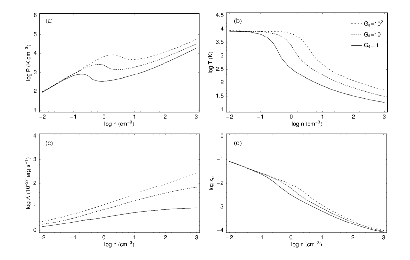
Figure 3: Overview of the ISM model for $\rm Z=Z_{\odot}/5$ (a typical metallicity for dwarf galaxies): equilibrium plots of (a) pressure $\rm P$, (b) temperature $\rm T$, (c) cooling rate $\rm\Lambda$ and (d) electron fraction $\rm x_{e}$ as a function of density $\rm n$ for three different values of the UV field $\rm G_{0}$ (given in units of $1.6\times 10^{-3}$ erg cm^-2 s^-1)

Our model for the ISM is similar to the equilibrium model of Wolfire et al. (1995, 2003) for the neutral phases and was extended from the more simplified models from Gerritsen & Icke (1997) and Bottema (2003). We consider a gas with arbitrary but fixed chemical abundances $\rm X_{i}$, scaled to the target metallicity from solar abundances. We solve for the ionization and thermal evolution of the gas. The thermal evolution is solved with a predictor/corrector step as in (Hernquist & Katz, 1989). The various processes included in the ISM model are given in Table 1. The main differences with the work of Gerritsen & Icke (1997) and Bottema (2003) are the following: we use more accurate cooling, that is calculated in accordance with the chemical composition, we solve for the ionization balance (albeit still assuming ionization equilibrium) and we use the full photoelectric heating efficiency as given in Wolfire et al. (1995). Indicatively, in Figure 3 we plot the equilibrium temperature, ionization fraction, heating (=cooling) and pressure as a function of density. There it can be seen that as density varies the equilibrium state of the gas changes from a high temperature/high ionization state ($\rm T=10^{4}~{}K$, $\rm x_{e}\approx 0.1$) at low densities, to a low temperature/low ionization state ($\rm T<100~{}K$, $\rm x_{e}<10^{-3}$) at high densities. In between there is a density domain where the negative slope of the P-n relation indicates that the gas is unstable to isobaric pressure variations, the classic thermal instability Field (1965). The shape of these curves and hence the exact densities of the thermal instability vary locally throughout the simulation, influenced by the time-varying UV radiation field and supernova heating. We set a constant cosmic ray ionization rate $\rm\zeta_{CR}$ throughout the galaxy, assumed to be $\rm\zeta_{CR}=3.6\times 10^{-17}~{}s^{-1}$.

Although we will consider models of different metallicities we will not consider the effects of abundance gradients or enrichment here. In general the abundance gradients observed in dwarf galaxies are small Pagel & Edmunds (1981), so this is a reasonable approximation. The fact that we keep the metallicity constant in time means that the model as presented here is not yet suitable to follow the evolution over cosmological timescales or to simulate very low metallicity dwarfs (for the simulations presented here the evolution in Z would be less than $10\%$ over the course of the simulation, even if no metals were to be lost to the intergalactic medium).

3.2 Star formation and feedback

The coldest and densest phase in our model is best identified with the CNM, where GMCs most likely form and remain embedded. We will use the simple prescription for star formation of Gerritsen & Icke (1997) as our standard star formation model. It was shown to reproduce the star formation properties of ordinary spiral galaxies and it is based on the assumption that the star formation process is governed by gravitational instability. A gaseous region is considered unstable to star formation if the local Jeans mass $\rm M_{J}$,

$$\rm M_{J}\equiv\frac{\pi\rho}{6}\left(\frac{\pi s^{2}}{G\rho}\right)^{3/2}<M_{ref}$$ (18)

(with s the sound speed), the assumption being that structure on a mass scale $\rm M_{ref}$ is present in the ISM. Once a region is dense and cold enough that (18) is fullfilled, the rate of star formation rate is set to scale with the local free fall time $\rm t_{ff}$:

$$\rm\tau_{sf}=f_{sf}t_{ff}=\frac{f_{sf}}{\sqrt{4\pi G\rho}}$$ (19)

The delay factor $\rm f_{sf}$ accounts for the fact that cloud collapse is inhibited by either small scale turbulence or magnetic fields Mac Low & Klessen (2004); Shu et al. (1987). Its value is uncertain and we consider values $\rm f_{sf}=2.5-20$. The actual implementation of star formation works as follows: once a gas particle is found to be unstable according to the Jeans mass criterion it can spawn a star particle with a mass one eighth of the mass of a gas particle (thus a given gas particle can produce at most eight star particles). The process is governed by either drawing from a Poisson distribution such that the local rate of star formation agrees with Eq. 19 in a stochastic sense, or by imposing a fixed delay time.

Our basic star formation recipe does not depend explicitly on the local H₂ fraction, so while the gravitational collapse that induces star formation may also precipitate H₂ formation, it is nevertheless independent of whether the gas is atomic or molecular. However, our model now allows for a direct link between star formation and the presence of molecular gas. We can do this by setting a local threshold for $\rm f_{m}$ above which star formation can proceed. As we will discuss in section 4.2.2 this may be more realistic since in such a scenario the values of the delay factor are no longer assumed a priori but are instead implemented in a more physical fashion by the “delay” associated with the final chemical/ thermodynamic evolution of a gas cloud before star formation.

In order to determine the local FUV field used for calculating the photoelectric heating and the H₂ destruction rates, we determine the time-dependent FUV luminosity of the stellar particles. We do so by following their age and, since star particles represent stellar associations rather than single stars, by using Bruzual & Charlot (1993 and updated) population synthesis models. We assume a Salpeter initial mass function (IMF) with cutoffs at $0.1\rm M_{\odot}$ and $\rm 100\rm M_{\odot}$. In the present work we do not account for dust extinction of UV light, except that of the young stars shrouded in their natal cloud: for a young stellar cluster we decrease the amount of UV extinction from 75% to 0% in 4 Myr Parravano et al. (2003).

Feedback from stellar winds and supernovae is essential for regulating the physical conditions of the ISM. While the mechanical energy output of stars is reasonably well known, it has proven to be difficult to include it completely self-consistently in galaxy-sized simulations of the ISM. The reason for this is that the effective energy of feedback depends sensitively on the energy radiated away in thin shells around the bubbles created. This will mean that the effect of feedback cannot be tracked in a straightforward manner unless prohibitively high resolution is used. In SPH codes there have been conventionally two ways to account for this: by changing the thermal energy input and by acting on particle velocities. Both are unsatisfactory, as the thermal method suffers from overcooling Katz (1992) and the kinetic method seems to be too efficient in stirring the ISM Navarro & White (1993). Here we use a new method based on the creation at the site of young stellar clusters of a pressure particle that acts as a normal SPH particle in the limit of the mass of the particle $\rm m\rightarrow 0$, for constant energy. For the energy injection rate (which assumes that the energy injection takes place continuously, without distinguishing between stellar winds and supernovae) we take

$$\rm\dot{E}=\epsilon_{sn}n_{sn}E_{sn}/\Delta t,$$ (20)

with $\rm E_{sn}=10^{51}$ erg the energy liberated per supernova, an efficiency parameter $\rm\epsilon_{sn}=0.1$, the number of supernova per mass of new stars formed $\rm n_{sn}=0.009$ per $\rm M_{\odot}$ (appropriate for the IMF adopted here) and $\rm\Delta t=3\times 10^{7}$ yr. The efficiency $\rm\epsilon_{sn}$ thus assumes that 90% of the initial supernova energy is radiated away in structures not resolved by our simulation. This value has been found in detailed simulations of the effects of supernovae and stellar winds on the ISM Silich et al. (1996); Thornton et al. (1998), and is also used in other simulations of galaxy evolution Semelin & Combes (2002); Springel & Hernquist (2002); Buonomo et al. (2000). Moreover in a study by Pelupessy et al. (2004) the adopted feedback strength has been shown to be consistent with the observed scatter in the star formation properties of isolated dwarf galaxies. Details of the feedback model, including implementation features and observational constraints can be found in Pelupessy et al. (2004) and Pelupessy (2005). The most important effect of SN feedback for our model of H₂ formation is, apart from the regulating effect of feedback on star formation, the introduction of extra dynamical pressure (Eq. 11) through the increases in local velocity dispersion.

3.3 H₂ formation

For our H₂ formation model we follow the same philosophy as for the star formation model: unresolved structure is assumed to be present at the SPH particle positions. In this case the underlying structures are assumed to conform to Eq. 10 expressing the mean extinction and derived from the observed density/size scaling relation (Eq. 8). However the latter is not expected to be valid throughout our simulation domain. Regions where the density/size relation becomes inapplicable are those with low density and pressure where it predicts very large cloud sizes and the resulting photo-destruction of H₂ proceeds very slowly. Such regions contain WNM HI gas where the pressure is mostly thermal and then Eq. 8 (along with $\rm P_{e}=n_{e}k_{B}T_{k}$) yields $\rm R_{pc}\propto T_{k}P_{e}^{-1/2}$, which for typical WNM conditions corresponds to kpc-size “clouds”. To circumvent this problem we modify Eq. 8 for $\rm P_{e}<P_{trans}$ as:

$$\rm\langle n\rangle=n_{\circ}\left(\frac{P_{trans}/k_{B}}{10^{4}\ K\ cm^{-3}}\right)^{-1/2}\left(\frac{P_{e}/k_{B}}{10^{4}\ K\ cm^{-3}}\right)R^{-1}_{pc},$$ (21)

where we take $\rm P_{trans}\approx 1000$ K cm^-3. This is just a convenient patch, which however in low pressure environments does scale the ”cloud” mean density as $\rm\propto P_{e}$, found for diffuse clouds Elmegreen (1993). This minor modification now allows the application of our subgrid model in all ISM conditions present in the simulations.

For the macroscopic pressure $\rm P_{e}$ in Eq. 11 we need the local velocity dispersion $\rm\sigma_{vel}$. For this we take the formal SPH estimate

$$\rm\sigma_{j}^{2}=\sum_{i}\frac{m_{i}}{\rho_{j}}(v_{i}-\langle v\rangle_{j})^{2}W(|r_{ij}|,h_{j})$$ (22)

with $\rm v_{i}$ and $\rm m_{i}$ the particle velocities and masses, $\rm\langle v\rangle_{j}$ the local bulk velocity. A number of subtle issues are connected with the choice of the dispersion. Equation 22 describes the inter-particle velocity dispersion, while the dispersion that enters Eq. 11 is really an intercloud velocity dispersion. Even if we assume these to be equivalent, the problem remains that Eq. 22 expresses a velocity dispersion on scales of the local SPH smoothing length $\rm h_{i}$. We can try to account for this by scaling $\rm\sigma_{j}$, using for example the relation for Kolmogorov turbulence,

$$\rm\sigma^{\prime}_{j}=\sigma_{j}\left(\frac{h_{j}}{R_{cloud}}\right)^{-1/3},$$ (23)

but we found this to have rather little influence on the resulting H₂ formation.

Depending on the cloud model, we use Eqs 12 or B5 when $\rm T_{k}\lesssim 1000\ K$ to track the evolution of $\rm A_{v}^{(tr)}$, and thus $\rm f_{m}$, during a simulation timestep dt. For $\rm T_{k}>1000\ K$ and $\rm R_{f}=0$ Eq. A3 describes the photodestruction of clouds, while for $\rm T_{k}>3000\ K$, Eq. 17 is used to approximate the collisional destruction process of the remnant molecular gas. The density that enters those equations is assumed to be the mean density $\rm\langle n\rangle$ given by the SPH density at the particle position, and the temperature the particle temperature (both taken constant for the timestep). The radiation field is calculated from the distribution of stars, where the assumption is that extinction from dust, or from molecular clouds is not important (apart from extinction from the natal cloud). After we have evolved $\rm A_{v}^{(tr)}$ for the timestep $\rm dt$ the resulting $\rm f_{m}$ (Eqs 7, B3) is calculated and assigned to the SPH particle for the duration of the next timestep (where it can be used to calculate e.g. cooling). At the next timestep the last $\rm f_{m}$ value is retained and used to calculate the initial $\rm A^{(tr)}_{v}$, given the new average cloud extinction $\rm\langle A_{v}\rangle$, which may have changed from the previous time-step, if for example the pressure $\rm P_{e}$ has changed.

The choice to keep $\rm f_{m}$ rather than $\rm A_{v}^{(tr)}$ constant during any variations of $\rm\langle A_{v}\rangle$ is dictated by the decision to assign all variations of $\rm f_{m}$ to the FUV-regulated HI/H₂ gas phase interplay, as tracked by Eqs 12 and B5 rather than to any instantaneous effects. Indeed, if $\rm A_{v}^{(tr)}$ instead of $\rm f_{m}$ was to be kept constant during variations of $\rm\langle A_{v}\rangle$ over a given time-step, it would correspond to an $\rm f_{m}$ that instantaneously follows the variations of $\rm\langle A_{v}\rangle$. This may not be entirely without merit since whatever processes are responsible for setting up cloud structures that obey power laws like that expressed by Eq. 8 may be also responsible for a fast concurrent H₂ formation Chièze & Des Forêts (1987); De Boisanger & Chiéze (1991). Nevertheless at this stage we chose not to consider this possibility since the cloud power laws are assumed “frozen” during our simulations and allowing instantaneous effects on $\rm f_{m}$ (via variations of $\rm\langle A_{v}\rangle$) would run counter to the spirit of our effort to model the time evolution of the HI, H₂ gas phases without such influences. In the future we intend to explore this possibility to see whether it is important when compared to the FUV-regulated HI/H₂ phase interplay explored here.

3.3.1 The applicability of the H₂ formation model at high resolutions

In order to track dense gas our simulations employ SPH particle masses of $\rm m_{SPH}=500\ M_{\odot}$ (see section 4.2.1) where it can be argued that the applicability of the scaling laws used to deduce $\rm f_{m}$ is doubtful because such small masses are well below those of even the smallest GMCs and thus represent cloud fragments instead. However, individual SPH particles do not represent the smallest resolved objects of our simulations, rather this is set by the total number of particles used to derive the formal SPH estimate of the mean density. The latter is of the order $\rm M_{ref}\sim\rm 10^{4}\ M_{\odot}$ (see Section 4.2), comparable to small molecular clouds. Furthermore, it must be noted that the applicability of the n-R scaling law for their $\rm M_{ref}$ sub-units is based on the virial theorem and the universality of the linewidth-size relation. The latter has now been confirmed to hold for scales and environments well inside typical molecular clouds and with the same normalizing constant as for entire clouds, a fact attributed to the universality of large-scale driving mechanisms for turbulence (Heyer & Brunt 2004). Regarding the virial theorem, it is a simple corollary that if GMCs are virialized objects so will be any of their sub-units albeit at different boundary pressures, thus Eqs 8, 10 are expected to hold even for $\rm M=M_{ref}$ cloud masses making up larger GMC-type ensembles ($\sim(10^{5}-10^{6})\rm M_{\odot}$). The latter of course assumes that the correct boundary pressure $\rm P_{e}$ is used in Eqs 8, 10, which as we already discussed may be poorly represented by the formal SPH estimate of the macroscopic velocity dispersion. Thus our model is applicable for scales where the size-linewidth relation and the assumption of virial equilibrium are valid, which will certainly not be the case in dense star forming cores, but does seem to be true at the larger scales as probed by galaxy scale simulations.

4 An application to dwarf galaxies

Our first application will be a model of a dwarf irregular galaxy. There are a number of practical reasons to choose this type of a system as a test model, as well as some interesting issues that are particular for dwarf galaxies that can be explored using our model (e.g. H₂ vs HI gas supply). The small size of these systems allow relatively high resolution with modest computational effort. Indeed the choice of dwarf galaxies as modeling templates allows a given numerical simulation to probe small physical scales and high gas densities, the latter being of crucial importance if the $\rm HI\rightarrow H_{2}$ phase transition is to be tracked successfully. Insight gained from simulating these systems, whose properties are constrained by a wealth of observational data (Van Zee 2001; Barone et al. 2000; de Paz, Madore & Pevunova 2003). Furthermore it holds the promise of yielding good constraints about physical processes that are expected to be universal in galaxies (see e.g. similar work done for SN feedback strength; Pelupessy, van der Werf, & Icke 2004).

Aside from being excellent testbeds for quantifying phenomena expected to be common across the Hubble sequence, dwarf galaxies are important systems on their own right because of their possibly very important role in current galaxy formation theories as the building “blocks” of larger systems Kauffmann et al. (1993), and as major “polluters” of the intergalactic medium with metals Ferrara & Tolstoy (2000).

4.1 Simulation setup

We construct a simple model of a dwarf irregular with gas mass of $\rm M_{gas}=10^{8}~{}M_{\odot}$ and a stellar mass of $\rm M_{star}=10^{8}~{}M_{\odot}$. Specifically, the gas disk has radial surface density profile

$$\rm\Sigma=\Sigma_{g}/(1+R/R_{g}),$$ (24)

with central density $\rm\Sigma_{g}=10~{}M_{\odot}/pc^{2}$ and radial scale $\rm R_{g}=0.33~{}kpc$, truncated at 4 kpc. An exponential stellar disk,

$$\rm\rho_{disk}(R,z)=\frac{\Sigma_{0}}{2h_{z}}\exp(-R/R_{d})sech^{2}(z/h_{z})$$ (25)

with central surface density $\rm\Sigma_{0}=300~{}M_{\odot}/pc^{2}$, $\rm R_{d}=0.5~{}kpc$ and vertical scale height $\rm h_{z}=0.2~{}kpc$, is constructed as in Kuijken & Dubinski (1995). The gaseous and stellar components are represented by $2\times 10^{5}$ particles each. For the gravitational softening length of the stellar particles a value of 20 pc is adopted, while for the gas particles it is taken to be equal to the SPH smoothing length. The ages of the initial population of stars are distributed according to a constant star formation rate (SFR) and an age of 13 Myr.

The rotation curves of dwarf galaxies are generally best fit using dark halos with a flat central core (Flores & Primack 1994, Burkert 1995). Therefore we take a halo profile

$$\rm\rho_{halo}(r)=\rho_{0}\frac{\exp(-r^{2}/r_{c}^{2})}{1+r^{2}/\gamma^{2}}$$ (26)

with core radius $\rm\gamma=2~{}kpc$, cutoff radius $\rm r_{c}=20~{}kpc$ and central density $\rm\rho_{0}=2\times 10^{7}~{}M_{\odot}/kpc^{3}$, for a total mass of $\rm M_{halo}=15\times 10^{9}\,M_{\odot}$ and a peak rotation velocity of about 50 km/s. Note that the profile adopted is very similar to the Burkert (1995) profile. They differ mainly in their asymptotic behaviour for $\rm r\to\infty$, thus the Burkert profile will only deviate significantly well outside the region of interest for our simulation (within 20 kpc the difference in rotation velocity of the adopted density profile and a Burkert profile with the same central density is $<6\%$). We represent the dark-matter halo by a static potential.

4.2 Practical considerations

The mass resolution of the simulation limits the density that can be probed. We can derive some minimum requirements in order for our model to be able to follow the $\rm HI\rightarrow H_{2}$ transition. In addition, it may be necessary to consider the effect of H₂ cooling. Finally, unlike previous numerical work reported in the literature, the range of values for the delay factor $\rm f_{sf}$, which regulates star formation, can now be explored under constraints imposed by the observationally-motivated demand that H₂ forms ahead of stars.

4.2.1 The necessary resolution: the choice of M_ref

Simulations of self-gravitating fluids done with insufficient numerical resolution can suffer from artifacts: artificial clumping or inhibition of gravitational collapse may occur. For SPH simulations including self-gravity these effects can arise if the local Jeans mass is not resolved (Bate & Burkert 1997; Whitworth 1998). Hence, this requires for our simulation

$$\rm M_{J}>Nm_{SPH},$$ (27)

with N the number of SPH neighbours and $\rm m_{SPH}$ is the mass of an SPH particle. In our simulations this requirement is met by choosing appropriate star formation parameters so that violation of Eq. 27 is precluded by star formation. A gas particle will “spawn” star particles, and thus be subjected to heating that raises the local Jeans mass, whenever $\rm M_{J}<M_{ref}$. Taking $\rm M_{ref}=Nm_{SPH}$ in effect makes the choice of mass (and density) resolution equivalent to the choice of $\rm M_{ref}$. The density resolution of our simulations must be high enough so that H₂ formation can compete with FUV dissociation (i.e. $\rm r_{dis}<1$, Eq. 13). In Figure 1 it is apparent that densities of $\rm\sim(50-100)\ cm^{-3}$ are sufficient to follow the $\rm HI\rightarrow H_{2}$ transition, while somewhat higher densities may be necessary for low metallicity gas. For such densities and at typical $\rm T_{k}(CNM)\sim 100\ K$, Eq. 18 yields $\rm M_{J}\approx 10^{4}\ M_{\odot}$. Hence running the simulation with particle masses of $\rm m_{SPH}\approx 500\ M_{\odot}$ allows a good resolution of the aforementioned mass scale. Apart from properly tracking the HI/H₂ phase transition, setting a small $\rm M_{ref}\sim 10^{4}\ M_{\odot}$ allows GMC-type, star-forming associations of gas particles to naturally emerge in the simulations. Indeed, GMC-class gas masses of $\rm M_{GMC}\sim(10^{5}-10^{6})\ M_{\odot}$ can then emerge as assemblies of smaller star-forming cloud units. Our star formation criterion $\rm M_{J}<M_{ref}$, where $\rm M_{ref}<M_{GMC}$, ensures that such self-gravitating SPH particle formations (which previous simulations show emerging, e.g. Gerritsen 1997) always contain gravitationally unstable regions that form stars, exactly as in real GMCs. In that respect $\rm M_{ref}$ can be viewed as a mass “radius” attached to individual SPH particles which defines the Jeans-mass instability, and which is itself smaller than the mass of typical GMC aggregates, the preferred sites of star formation in galaxies. If one were to choose $\rm M_{ref}\gg M_{GMC}$ stars could then form from “cloud” mass scales that are never seen star forming in nature. As a final note on the choice of $\rm M_{ref}$ it worths mentioning that observational studies have shown that O, B stars do not form in GMCs with masses below $\sim 10^{5}\rm\ M_{\odot}$ (Elmegreen 1990). Thus choosing $\rm M_{ref}\sim 10^{4}\ M_{\odot}$ makes our simulations capable of following the evolution of the smallest GMCs seen forming stars in galaxies.

4.2.2 The choice of $\rm f_{sf}$: the role of H₂ and star formation

In our standard star formation recipe the delay for star formation to occur is set by the free parameter $\rm f_{sf}$; our default choice is a fixed value of $\rm f_{sf}=10$. In the past typical values of $\rm f_{sf}\sim 5-10$ were chosen so that the expected star formation rate from the GMCs present e.g. in the Milky Way would be similar to the one observed. Dedicated high-resolution simulations of individual molecular clouds may shed some light on this issue (e.g. MacLow et al 1998), but for the time being the choice of $\rm f_{sf}$ in galaxy-size simulations like ours remains rather apriori.

Nevertheless the fact that everywhere in the local Universe stars seem to form out of molecular rather than atomic gas allows us to deduce a lower limit on the value of $\rm f_{sf}$. Indeed, for H₂ formation to remain always ahead of star formation it must be $\rm\tau_{f}(H_{2})\leq\tau_{sf}$, which from Eqs 2 and 19 yields,

$$\rm f_{sf}\gtrsim 5.33\left(\frac{\langle n_{1}\rangle}{cm^{-3}}\right)^{-1/2}\left(\frac{\mu Z}{3.5}\right)^{-1}\left[\frac{(1+T_{k}/100~{}K)^{2}}{(T_{k}/100~{}K)^{1/2}}\right].$$ (28)

Since CNM HI is the most likely precursor phase of the H₂ gas, for typical conditions of $\rm T_{k}\sim(100-200)\ K$ and $\rm\langle n_{1}\rangle\sim(10-50)cm^{-3}$, the latter equation yields $\rm f_{sf}\gtrsim 3-10$. These values are roughly similar to those deduced using the constraints on the observed star formation rate in the Galaxy. Given the uncertainties inherent in e.g. the $\rm S_{H}(T_{k})$ function, such a rough agreement is noteworthy and here it is worth mentioning that $\rm\tau_{f}(H_{2})$ is also a good approximation of chemical equilibrium timescales in FUV-illuminated clouds Hollenbach & Tielens (1999). Thus the rough agreement of the constraint set by Eq. 28 with what are considered reasonable $\rm f_{sf}$ values may signify an important role for cloud chemistry in setting the average star formation rate. This is not far-fetched since molecule formation enables very different gas cooling functions and thus drastically alters its thermodynamic state allowing to eventually cool and fragment further (well beyond the resolution limit for galaxy-sized simulations) (e.g. Chiéze & des Forêts 1987). For these reasons we will also discuss a model for the star formation which depends on $\rm f_{m}$ directly.

4.2.3 Cooling by H₂

A detailed calculation of H₂ cooling was done by Le Bourlot et al. (1999). At $\rm T_{k}\sim(1000-8000)K$ H₂ is a more efficient coolant than the other major coolants (C and Fe). Hence even a low ($\sim 10^{-4}$) remnant abundance of molecular gas in the diffuse WNM can have an impact on the cooling at these temperatures. Indeed some people have included H₂ cooling in their cooling curves, but without calculating the abundance of molecules Carraro et al. (1998). Admittedly our accuracy in following the amount of warm molecular gas is limited, but to get some idea of the possible effect of such a gas phase it is nevertheless interesting to do some calculations including H₂ cooling. For this we use the Le Bourlot cooling curve, where we use a limited set of data (low density limit, constant ortho-to-para ratio, only H₂-H collision excitation), appropriate for our purposes. Note that some observations find abundances of H₂ gas the order of $10^{-4}-10^{-3}$ in diffuse HI gas, even in regions of the ISM hostile to H₂ formation, like galactic high velocity clouds Richter et al. (2001).

5 Dwarf galaxy model: results

In a model that incorporates H₂ formation the two obviously important parameters that should be explored are: the formation rate $\mu$, and the metallicity Z. The formation rate is uncertain by a factor of 5-10, and thus introduces some uncertainty in the theoretically calculated H₂ content, e.g. for high formation rates significant amounts of warm and diffuse H₂ may be present in the outer parts of spiral galaxies (Papadopoulos, Thi, & Viti 2002). Metals play an important role: the H₂ formation rate is directly proportional to the dust surface available, and we take this surface to be proportional to Z. Dust also plays an important role shielding molecules from UV radiation. Observations of low metallicity systems, like dwarf irregulars, using CO as a tracer give low molecular gas contents Barone et al. (2000). However, the interpretation of these observations is complicated by the fact that the conversion factor from CO flux to H₂ mass under these conditions depends heavily on metallicity and ambient FUV field: for low metallicity, FUV-intense environments CO dissociates while the largely self-shielding H₂ is not affected by much Maloney & Black (1988); Israel (1997).

In this work we explore a 2x2 grid of models using a formation rate of $\mu=3.5$ and $\mu=17.5$, and metallicities of either $\rm Z=Z_{\odot}/5$ or $\rm Z=Z_{\odot}$. Note that for our model dwarf galaxy the high metallicity is somewhat unrealistic, because normally dwarf galaxies have lower metal content. Note also that for simulations without H₂ cooling our subgrid model follows the H₂ content as a passive tracer of the history of the local conditions, thus the simulations for high and low formation rate will be identical except for the amount of H₂.

5.1 Star formation properties of the simulations

We start the simulation with an isothermal gas disk at $\rm T_{k}\approx 8000~{}K$, and a molecular fraction $\rm f_{m}=0$. After the start of the simulation the gas cools and collapses along the z-direction, forming regions of cold and dense gas in the midplane (the minimum size of structures resolved in the simulation is about 30 pc). There, H₂ starts to form and star formation starts taking place as well. The fact that we start from an unrealistically smooth initial condition results in some transient effects, but after approximately 200 Myr the galaxies settle in a stationary state, with a constant star formation (see Figure 4). For this model galaxy, the mean star formation rate is about $\rm SFR=0.002~{}M_{\odot}/yr$ for low Z and $\rm SFR=0.003~{}M_{\odot}/yr$ for high Z, with modest variations (the gas depletion timescale is much longer than the duration of our simulation, in the order of $5\times 10^{10}$ yr). The star formation values we get represent fairly typical values for a low surface brightness dwarf Van Zee (2001). Also plotted in Figure 4 is the average star formation density as a function of radius, note the exponential distribution of star formation and the sudden truncation. During the simulation a small fraction ($1\times 10^{-3}$) of the gas is expelled out of the disk, but most of this falls back. A hot galactic wind is not formed, the low mass loss rate associated with the expected wind for this model cannot be resolved by our current mass resolution.

5.2 Spatial and temporal distribution of H₂ gas

An equilibrium fraction of H₂ is reached on timescales of $\approx 50-100$ Myr (see Figure 5), in agreement with our earlier approximate estimates from Eq. 2. Furthermore, as expected, the low-$\mu$/low-Z simulation yields the lowest equilibrium molecular fraction of $\rm f_{m}\sim 0.001$ and a higher formation rate $\mu=17.5$ will boost that to $\rm f_{m}\sim 0.03$. For high metallicities, molecular fractions of $\rm f_{m}\sim 0.17$ ($\mu=3.5$) and $\rm f_{m}\sim 0.4$ ($\mu=17.5$) form. Also drawn in Figure 5 is the time dependence of the molecular fraction for a low-$\mu$/low-Z simulation with logotropic clouds. The difference between constant density and logotropic clouds is not very large, certainly smaller than the differences due to the uncertainties of $\mu$ (this is also evident in the equilibrium values of $\rm f_{m}$ shown in the panels in Figure 1, where the main difference between constant density and logotropic clouds was that for logotropic clouds appreciable fractions $\rm f_{m}$ appear also at lower densities).

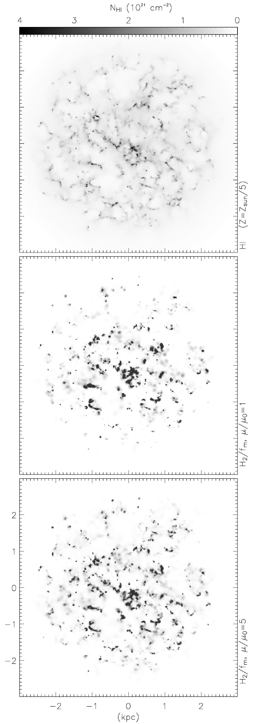
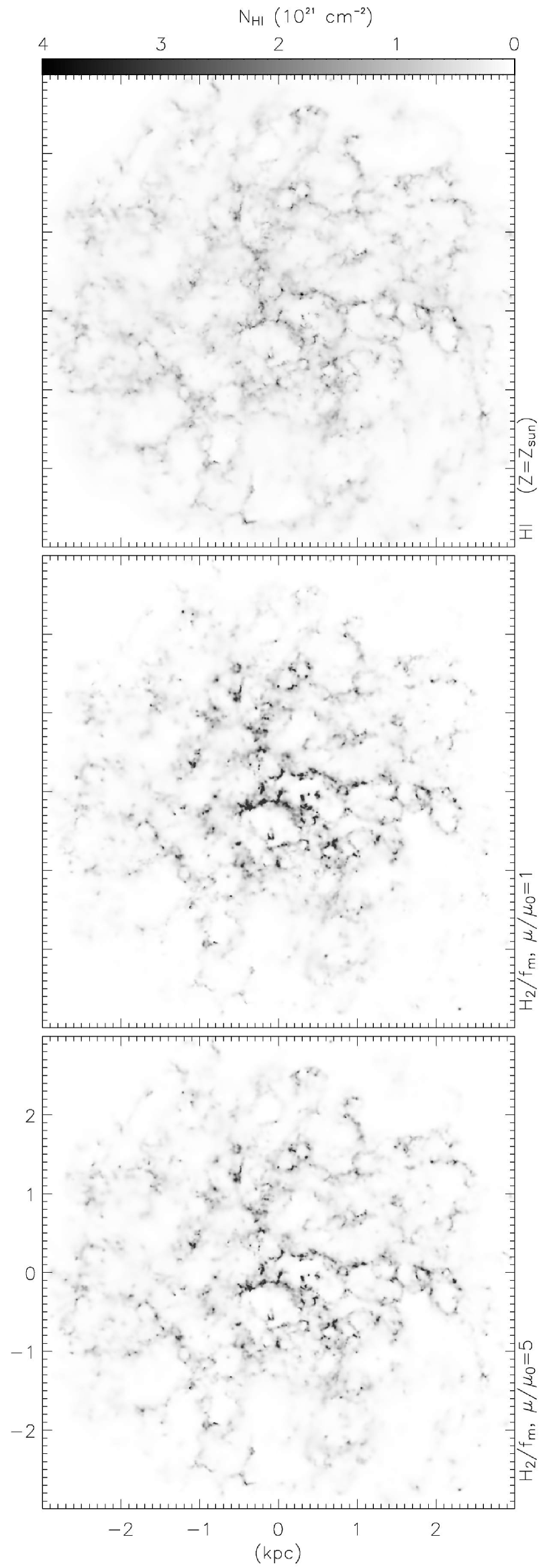
Figure 8: HI and H₂ maps. Left panels: results for $\rm Z=Z_{\odot}/5$, right panels: $\rm Z=Z_{\odot}$. Shown are, from top to bottom, the HI distribution, the H₂ distribution for $\mu=3.5$ and for $\mu=17.5$. The HI maps of low and high $\mu$ simulations are very similar, shown are only the maps for $\mu=3.5$. The H₂ maps have been dividided by the global molecular fraction such that the differences with the HI distribution can be seen more clearly.

In Figures 6 and 7 we show the (mean) molecular fraction as a function of radius and height above the disk-plane for the four simulations. We see that, as expected, H₂ forms mostly in the central regions and in the midplane where the pressure and gas density builds up. Note also that for high metallicity and high formation rate the molecular fraction seems to have a tendency to ”saturate” in the central regions at a fixed value, in this case $\rm f_{m}=0.6$. Looking in more detail at the spatial distribution of HI and H₂ shown in Figure 8 we find H₂ mainly concentrated in the dense clumps and filaments of the HI distribution. The structure of the ISM can be quantitatively compared with observations by analyzing the power spectrum of the HI maps such as those in Figure 8. This is done in Figure 9, where we see that it agrees quite well with power spectra made for the most detailed studied dwarf galaxy, the Large Magellanic Cloud (LMC), and is stable over the course of the simulation and as a function of resolution. If we now compare the low and high $\mu$ simulations, we see similar H₂ distributions: the uncertainty in the formation parameter is mainly an uncertainty in the amount of H₂ formed, not in the locations of H₂ formation. The relative distribution of H₂ is well represented by our simulation, but the exact amount of H₂ is more difficult to determine, as this depends on the formation rate parameter. If we look at the high metallicity simulations, we can see that, apart from the clumpy distribution there is also a sizable mass of ”diffuse” H₂, but still confined mainly in gas filaments.

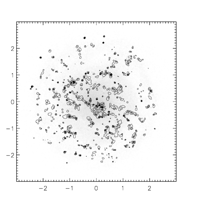
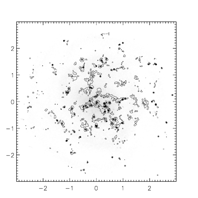
Figure 10: H$\alpha$ and H₂: simulated H$\alpha$ maps with H₂ contours. Left panel shows the maps for the $\rm Z=Z_{\odot}/5$, $\mu=3.5$ simulation (contours at column densities of $\rm N_{HI}=2\times 10^{19}$ and $10^{20}$ cm^-2) while the right panel shows the $\rm Z=Z_{\odot}$, $\mu=17.5$ run (contours at column densities of $\rm N_{HI}=2\times 10^{20}$ and $10^{21}$ cm^-2).

Finally we look at the relation between star formation and H₂ distribution. In Figure 10 we show a simulated ”H$\alpha$” map (actually a map of the stellar luminosity in ionizing photons), overplotted with contours of H₂ gas, chosen so that they highlight the relation of star formation to the densest parts of the H₂ distribution. It can be seen that star formation is almost always associated with some nearby H₂ gas complex while some of them, being without newly formed stars at that particular instant, do not show any H$\alpha$ emission.

5.3 The influence of the collapse delay factor $\rm f_{sf}$

Apart from the parameters directly related to H₂ formation, $\rm f_{m}$ will also depend on the delay factor $\rm f_{sf}$. As discussed in section 4.2.2, this parameter accounts for the fact that a region that is Jeans-unstable does not collapse to form stars at the free-fall time $\rm\tau_{ff}$. The total amount of H₂ is sensitive to the time HI gas stays in a cold and dense phase conducive to H₂ formation, while the emergence of new stars from such a phase helps dissociate H₂ by dramatically increasing the ambient FUV radiation. Indeed, comparing models run with different values for $\rm f_{sf}$ reveals the total amount of molecular gas to be strongly dependent on this parameter (Figure 11). In short, the formation of stars and H₂ are in competition, and small enough delay factors can quench H₂ formation. Yet, a value of $\rm f_{sf}\gtrsim 10$, as constrained by the observed GMC masses and the star formation rate in the Galaxy, amply satisfy Eq. 28 and H₂ formation preceeds star formation.

5.4 Star formation with an H₂ gas fraction threshold

In section 4.2.2 we have argued for a connection between star formation and chemical timescales, the latter well approximated by the H₂ formation timescale. A simple and direct implementation of this idea is to replace the preset delay time $\rm\tau_{sf}$ by a threshold molecular fraction $\rm f_{m,sf}$ for the onset of star formation. In this case the delay factor $\rm f_{sf}$ is no longer needed; the “delay” from a pure free-fall timescale is now the outcome of the interplay between the competing physical processes that lie behind the establishment of $\rm f_{m}$.

We rerun the $\rm Z=Z_{\odot},\mu=3.5$ simulation with this new star formation recipe and a threshold value of $\rm f_{m,sf}=1/8$. In figure 11 we have plotted $\rm f_{m}$ for this case. As can be seen, the equilibrium molecular fraction goes down significantly, to $\rm f_{m}\approx 0.01$, which is easily understood, because such a low threshold value will almost immediately destroy H₂ once it forms. For higher threshold values $\rm f_{m}$ is higher, $\rm f_{m}\approx 0.05$ and $0.1$ for $\rm f_{m,sf}=3/8$ and $5/8$ respectively (this is still less than for the normal recipe, because for this case about $40\%$ of H₂ is in regions with $\rm f_{m}>5/8$). The star formation rate for these models is about $\rm SFR=0.004~{}M_{\odot}/yr$.

In figure 12 we plot the resulting (cumulative) distribution of delay times $\rm\tau_{sf}$, normalized on the local free-fall time $\rm t_{ff}$. A higher threshold results in longer average delay times, from $\rm\langle\tau_{sf}\rangle\approx 1.5t_{ff}$ for $\rm f_{m,sf}=1/8$ to $\rm\langle\tau_{sf}\rangle\approx 10t_{ff}$ for $\rm f_{m,sf}=5/8$. However, the fraction with $\rm\tau_{sf}<t_{ff}$ stays roughly constant. The reason for this is that once star formation starts in a region, it takes some time for feedback to kick in. In the mean time molecule formation continues, and the molecular regulated star formation allows for extra star formation events if enough H₂ forms (in the previous implementation of star formation there was no such possibility). In other words, the local star formation efficiency is partly determined by the H₂ formation.

A high value for $\rm f_{m,sf}$ seems to be favoured, because star formation regions are observed to be mainly molecular, and in this case both the H₂ fractions and local star formation rates are consistent with what is known from observations. Hence this model for star formation seems promising for future application.

5.5 Simulations with H₂ cooling

The inclusion of H₂ cooling affects the simulation in a number of ways. As an extra coolant it will increase the amount of gas in a cold state, and in turn this will increase the formation of H₂. However, star formation will also increase, and thus also the UV field. In Figure 13 the effect of cooling on $\rm f_{m}$ is illustrated for the $\mu=3.5$ simulations. As can be seen, cooling has some influence for the high Z simulation but for low Z the molecular fractions are too low to substantially alter the results. Note that while H₂ is a strong coolant at high temperatures (a few thousand K), where it dominates the cooling for $\rm f_{m}>0.001$, the effect of the extra cooling is limited because of the small amount of gas at these temperatures.

6 Discussion

Detection and mapping of the molecular component of dwarf galaxies is usually done by mapping the $\rm{}^{12}CO(J=1-0)$ line Barone et al. (2000); Mizuno et al. (2001) or by UV absorption studies (Tumlinson et al. 2002). The derived H₂ fractions are $\sim(1-10)\%$, but for low metallicity systems CO is often not detected corresponding to upper limits for the molecular fraction of $\sim 1\%$. Recently a large observational effort has detected ¹²CO J=1–0 in several more dwarf galaxies increasing the number of such systems with detected CO emission by $\sim 50\%$ (Leroy et al. 2005).

At this stage a direct comparison of our simulations with available CO imaging data must be made cautiously. This is because our simulations follow the formation of H₂ not CO. The latter is the most abundant molecule after H₂ itself and serves as the prime tracer of its mass (e.g. Dickman, Snell, & Schloerb 1986; Young & Scoville 1991), yet it is still four orders of magnitude less abundant and thus, unlike H₂, it cannot self-shield. This is the main reason why in metal-poor and FUV-intense environments like those prevailing in dwarf galaxies CO (but not H₂) will be dissociated and its emission can then give a rather misleading picture of the H₂ mass distribution (e.g. Madden et al. 1997). Even if a simplified version of the chemical network giving rise to CO (e.g. Nelson & Langer 1997) were to be included in the simulations, densities $\rm n\gtrsim 500\ cm^{-3}$ and temperatures $\rm T_{k}<50\ K$ would have to be tracked in order to successfully model CO formation, and these are currently inaccessible by galaxy-size simulations like ours.

In principle one could use empirical relations of the $\rm X=M(H_{2})/L_{co(1-0)}=F(G_{\circ},Z,n,T_{k})$ factor available from the literature (e.g. Israel 1997; Bryant & Scoville 1996), and then convert the H₂ maps from our simulations to CO brightness maps. This we intent to do in future work that will also include spiral disks. Nonetheless, the molecular fractions we derive here seem to be reasonable, although for the low-$\mu$/low-Z simulations the derived $\rm f_{m}$ is on the low side. The molecular fraction may increase somewhat for a simulation run at higher resolution, because in metal-poor environments the $\rm HI\to H_{2}$ transition is taking place above $\rm n=100~{}cm^{-3}$, this can increase $\rm f_{m}$ by a factor 2-5. For the galaxy models run with high metallicity and/or formation rate we find quite substantial fractions of H₂, of $\rm f_{m}=0.17-0.4$.

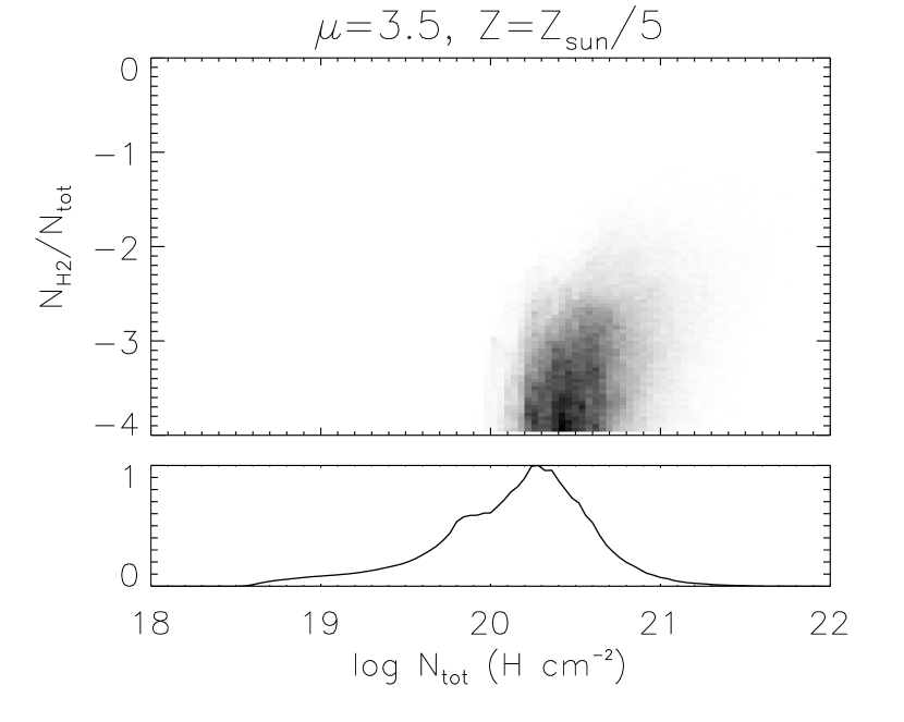
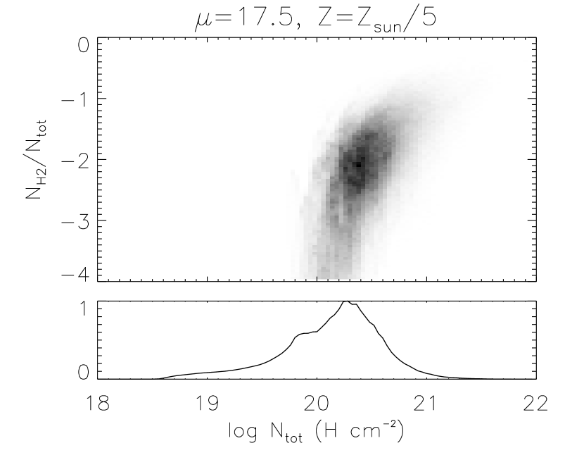
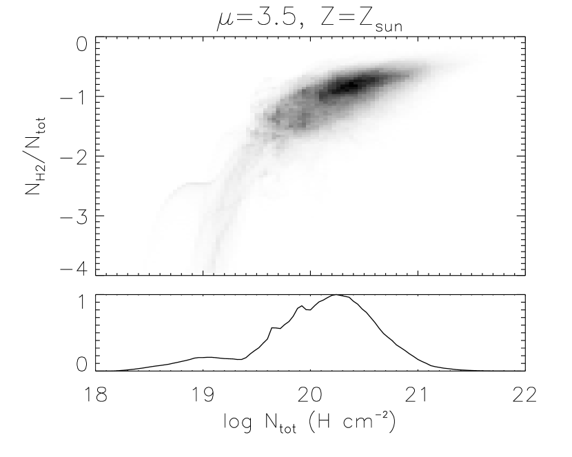
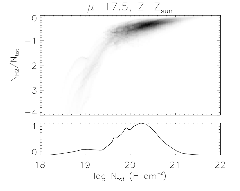
Figure 14: Fraction of H₂ vs total column densities. Gray scales give the distribution of H₂ fraction $\rm N_{H_{2}}/N_{HI}$ and total column density $\rm N_{HI+H_{2}}$ of the pixels of HI and H₂ projection maps. Histograms give the distribution of pixel values of the total column density, scaled to the maximum bin.

We also seem to find quite high values, $\rm f_{H_{2}}\approx 0.001-0.01$, of the diffuse warm neutral medium to be molecular. To illustrate this we have plotted in Figure 14 the molecular fraction as a function of total column density for a face-on projection. There is a clear column density threshold for the presence of H₂ for the low metallicity simulation. For high metallicity even low column density regions (which are also of low density and high temperature) show fractions of $\rm f_{m}\approx 0.001-0.01$. This state of the gas (low density, high temperature) is not typically associated with the presence of such quantities of H₂. There is no - or very little - formation of molecular gas going on in this gas phase and any $\rm H_{2}$ present should dissociate. In fact, destruction is taking place in the simulation, but its timescales are quite long. For the thermal dissociation this is due to the low density of the gas: for temperatures of $\rm T=5000~{}K$ and density of $\rm n_{H}=0.3\ cm^{-3}$ the collisional destruction timescale (for neutral gas) is $\rm\tau_{col}\approx 10^{8}~{}yr$. Furthermore, for our model galaxy the radiation fields in quiescent regions are quite low, $\rm G_{0}\lesssim 0.1$, due to the low star formation, so the radiative dissociation timescales are also in the order of $\rm\tau_{rad}=1.3/G_{0}\times 10^{7}~{}yr\approx 10^{8}~{}yr$. Hence the H₂ survival in lukewarm gas may not be unrealistic. Note however that the simulation may not represent the dispersion of H₂ from dense regions realistically: molecular gas is formed in dense, star forming regions, where radiation fields are higher (for our model up to $\rm G_{0}=100$. As the star formation heats the surrounding gas it will destroy H₂, the amount of molecular gas that ”escapes” destruction is then sensitive to e.g. the time it is exposed to the high radiation field or the combination of high density/ high temperature. Also, destruction by supernova shock is not represented very well, because the interaction of the supernova shocks with the (sub resolution) molecular clouds is absent. On the other hand shocks have been shown recently to also induce fast H₂ formation as they propagate through diffuse HI gas (Bergin et al. 2004) and the effect of such a mechanism in the overall HI/H₂ balance in our simulations is unknown.

Nevertheless, our simulations do indicate that in so far as the molecular gas is not destroyed at the sites of its original assembly, it can survive the CNM-to-WNM transition. In that case the lukewarm and WNM gas phases may still contain significant amounts of H₂. In subsequent work we intend to explore the issue of H₂ survivability under such conditions more thoroughly by introducing a better model of its collisional and FUV-induced destruction in such gas phases while also including shock-induced H₂ formation and destruction mechanisms. Finally, any significant underlying cloud substructure in CNM HI clouds is likely to enhance the amount of H₂ gas present in that phase.

Future applications of H₂-tracking numerical models of galaxies can be divided in two broad and complementary categories, namely: a) examine the effects of the various model parameters on the H₂ distribution within a given galaxy by e.g. using different H₂ formation functions (see Cazaux & Tielens 2004), and/or using a range of $\rm f_{sf}$, $\rm\epsilon_{SF}$ and $\rm M_{ref}$ values, b) explore the evolution of the H₂/HI distribution across the Hubble sequence using a single “mean” H₂-tracking model. In the latter category starbursts/mergers, with their extreme and fast-evolving pressure and radiation environments (and hence probably strongly varying H₂/HI fractions) provide particularly attractive templates for modeling.

7 Conclusions

We presented a method to calculate the local H₂ content in simulations of the ISM based on a subgrid model for the formation and destruction of molecular gas. The model tracks the formation of H₂ on dust grains and its destruction by UV irradiation in the CNM phase and its collisional destruction in the WNM phase including the effects of shielding by dust and H₂ self-shielding. The solution to the H₂ formation/destruction problem is simplified greatly by the assumption that H₂ formation takes place in structures that conform to the observed density/size scaling relations, present on scales not resolved by the hydrodynamic code of the simulation. We show steady state solutions of the model for the molecular fraction $\rm f_{m}$ as a function of the average gas density, temperature, velocity dispersion, radiation field, and metallicity. The effects of the cloud substructure are explored by taking $\rm 1/r$ density profiles for the model clouds, this seem to have only a modest effect on the derived H₂ fractions, but it does allow more diffuse gas to be molecular.

A simple time-dependent formulation of the same model is then coupled to hydrodynamic simulations and used to calculate the local evolution of the molecular gas fraction according to the local macroscopic quantities. We have then incorporated our H₂-tracking method in an N-body/SPH code for the simulation of galaxy-sized objects. Our first application is to model a typical low surface brightness dwarf galaxy where the demands set by the density resolution necessary to properly track the $\rm HI\rightarrow H_{2}$ transition are easily met. Our results can be summarized as follows:

• We found that our model reproduces reasonable molecular fractions ranging from $\rm f_{m}=0.001-0.03$ for low metallicity to $\rm f_{m}=0.17-0.4$ for solar metallicity systems, saturating to $\rm f_{m}=0.6$ for high values of the H₂ formation rate and in the central regions of our model galaxies.

• The biggest uncertainty is the value of the adopted formation rate parameter $\mu$, however the general features of the spatial H₂ distribution do not depend significantly on $\mu$.

• The molecular fraction shows a strong dependence on the metallicity Z, as expected for H₂ forming on dust grains. Our model for a high metallicity dwarf shows surprising amounts of ”diffuse” H₂, possibly due to the low radiation fields outside star forming regions. This may be analogous to what happens in the outer regions of spiral galaxies where the radiation field drops, and a diffuse H₂ gas phase may be present there. However a better model for the H₂ formation and destruction in the WNM phase is needed before the aforementioned results can be considered secure.

• The molecular gas content is sensitive to the details of our star formation recipe, especially on the value of the delay factor $\rm f_{sf}$ adopted. This poorly constrained factor, generally used to parameterize a slower-than-free fall star formation timescale, needs to be sufficiently large, $\rm f_{sf}\gtrsim 10$ to allow for H₂ formation before young stars start to dissociate H₂. On the other hand a star formation criterion based on the formation of H₂ can dispense with the $\rm f_{sf}$ factor completely, giving local star formation rates well within constraints set by observations. This suggests that the star formation is governed by cloud chemistry processes, and indicates the importance of considering molecular gas in simulations.

• H₂ cooling has only a minor impact for our model. The largest effect of H₂ cooling is seen in high metalicity (and thus H₂ content) environments.

Summarizing, we developed an algorithm to calculate the evolution of the molecular gas phase during the evolution of the gaseous and stellar content of galaxies, and obtained a first application to dwarf galaxies. Strong points are that it is simple, physically motivated and not computationally expensive. It is well suited to galaxy-sized simulations where a complete treatment of the physics involved in the formation of the H₂ clouds is inaccessible, while our approach can be seen as complementary of (much higher resolution) simulations modeling individual molecular clouds. The set of astrophysical questions that can be addressed using such H₂-tracking models is large. These include examining the influence of “micro”-physics parameters/functions like the H₂ formation rate on the general molecular gas distribution within a given galaxy, as well as modeling the gaseous ISM evolution for galaxies across the Hubble sequence. The latter can now be done by including all gas phases along with the stars, with the molecular phase expected to be the most intimately involved with the star formation. Finally, mergers/starbursts, with their fast-evolving pressure and radiation environments are ideal templates for future applications of the model presented here.

Appendix A Analytical approximations for $\rm A^{(tr)}$

It is interesting to examine approximate analytical solutions of Eq. 12, if only for the reason of checking the more general solution in limiting cases. This can be done for two particular domains, namely that of rapidly increasing and rapidly decreasing $\rm A^{(tr)}_{FUV}(t)$. For $\rm\tau_{f}dA^{(tr)}_{FUV}/dt\ll 0$ we can approximate Eq. 12 as

$$\rm\frac{dA^{(tr)}_{FUV}}{dt}=-\frac{1}{\tau_{f}}A^{(tr)}_{FUV}\Rightarrow A^{(tr)}_{FUV}=A^{(tr)}_{FUV}(0)e^{-t/\tau_{f}}.$$ (A1)

In the case of $\rm\tau_{f}dA^{(tr)}_{FUV}/dt\gg 1$, and thus a decreasing molecular mass fraction, we approximate Eq. 12 as

$$\rm\frac{dA^{(tr)}_{FUV}}{dt}=\frac{r_{dis}}{\tau_{f}}e^{-A^{(tr)}_{FUV}}=2G_{\circ}k_{\circ}\Phi e^{-A^{(tr)}_{FUV}},$$ (A2)

hence

$$\rm A^{(tr)}_{FUV}(t)=ln\left(e^{A^{(tr)}_{FUV}(0)}+2G_{\circ}k_{\circ}\Phi t\right),$$ (A3)

which, for $\rm R_{f}=0$, provides a convenient solution describing the photo-destruction of molecular clouds.

Appendix B logotropic clouds

Here we give the corresponding equations of section 2 for clouds with a density profile $\rm n(r)=n_{e}(r/R)^{-1}$ (“logotropic clouds”). For a radially incident interstellar radiation field, such a density profile yields

$$\rm N_{tr}(HI)=\frac{\nu_{\circ}}{\sigma}ln\left(1+\nu^{-1}_{\circ}\frac{G_{\circ}k_{\circ}}{n_{e}R_{f}}\Phi\right),$$ (B1)

where $\rm\nu_{\circ}=n_{e}R\sigma\left(1+n_{e}R\sigma\right)^{-1}$. For $\rm R\rightarrow\infty$ we obtain $\nu_{\circ}\rightarrow 1$ and the transition column density of Eq. B1 reduces that of Eq. 4 (for $\rm n(r)\rightarrow n_{e}$), as expected, because for large clouds the density will not change much over $\rm N_{tr}(HI)$. The visual extinction corresponding to this $\rm N_{tr}(HI)$ is given by

$$\rm A_{v}^{(tr)}=1.086\nu_{\circ}\xi^{-1}_{FUV}\ln\left[1+\frac{\nu^{-1}_{\circ}G_{\circ}}{\mu S_{H}(T_{k})}\left(\frac{\xi_{FUV}}{ZT_{k}}\right)^{1/2}\left(\frac{n_{e}}{135\ cm^{-3}}\right)^{-1}\right].$$ (B2)

and the H₂ fraction $\rm f_{m}$,

$$\rm f_{m}\equiv\frac{M(H_{2})}{M_{c}}=exp\left[-4\frac{A_{v}^{(tr)}}{\langle A_{v}\rangle}\right].$$ (B3)

The modification of Eq. 12 for the time dependent transition column in the case of a logotropic density profile (Eq. 22 of Goldshmidt & Sternberg 1995) turns out to be particularly simple, namely

$$\rm\frac{1}{2}\frac{dN(HI,t)}{dt}=\frac{G_{\circ}k_{\circ}\Phi}{\sigma}e^{-\sigma N(HI,t)}-R_{f}\int_{0}^{r_{HI}}n(r)n(HI)dr.$$ (B4)

Here $\rm r_{HI}$ marks the depth of the HI layer. Using the relation $\rm n(r)=n_{e}e^{N(r)/N_{\circ}}$ ($\rm N_{\circ}=n_{e}R$) valid for a logotropic density profile, Eq. B4 eventually yields

$$\rm\tau_{f}\frac{d\sigma N_{tr}(HI,t)}{dt}=r_{dis}e^{-\sigma N_{tr}(HI,t)}-\sigma N_{\circ}\left(e^{\sigma N_{tr}(HI,t)/\sigma N_{\circ}}-1\right),$$ (B5)

where $\rm\tau_{f}$ and $\rm r_{dis}$ are calculated for $\rm n=n_{e}$. It can be easily seen that for $\rm N_{\circ}=n_{e}R\rightarrow~{}\infty$ B5 reverts back to Eq. 12 with a density $\rm n=n_{e}$ (i.e. the case of a cloud with so large a radius that the HI/H₂ equilibrium is well approximated by a plane-parallel geometry at a uniform density $\rm n=n_{e}$).

For $\rm dA^{(tr)}_{FUV}(t)/dt\gg 0$ the solution of Eq. B5 remains the same as in Eq. 12 but with $\rm n_{e}=2/3\langle n\rangle$ replacing n. Hence, in the case of cloud destruction and $\rm R_{f}=0$, Eq. A3 expresses the time dependence of the transition layer also in logotropic clouds. For $\rm dA^{(tr)}_{FUV}(t)/dt\ll 0$, Eq. B5 is now approximated by

$$\rm\tau_{f}\frac{dA^{(tr)}_{FUV}(t)}{dt}=-A_{\circ}\left[e^{A^{(tr)}_{FUV}(t)/A_{\circ}}-1\right],$$ (B6)

($\rm A_{\circ}=\sigma N_{\circ}$), with the solution of the latter being

$$\rm A^{(tr)}_{FUV}(t)=A_{\circ}ln\left[1+(e^{A^{(tr)}_{FUV}(0)/A_{\circ}}-1)e^{-t/\tau_{f}}\right].$$ (B7)

The latter expression reduces to that in A1 when $\rm N_{\circ}\rightarrow\infty$ ($\rm A_{\circ}\rightarrow\infty$), as expected.

Figure 1: The equilibrium molecular fraction $\rm f_{m}$. Plotted are contours (labelled with the corresponding value) of $\rm f_{m}$ for various representative combinations of formation rate parameter $\mu$, cloud power law index $\alpha$, metallicity Z, radiation field $\rm G_{0}$ and velocity dispersion $\rm v_{disp}$ (Actual values are indicated in the plots). Above 1000 K the formation rate is taken to be zero. $\alpha$ indicates the power law index of the density profile ($\rm n\propto r^{-\alpha}$), thus $\alpha=0$ means constant density clouds, $\alpha=1$ logotropic clouds.

Figure 2: Comparison of the solution of Eq. 12 for the photodissociation of a molecular (plane-parallel) cloud and the solution of Goldshmidt & Sternberg (1995) of the full integro-differential equations. Plotted is the total HI column N(HI) as a function of time since the onset of FUV irradiation (normalized on $\tau_{f}$) where the drawn lines are the solutions of our Eq. 12 for different values of the Goldshmidt & Sternberg (1995) $\alpha$ parameter ($\alpha\Phi=\rm r_{dis}$) while the dashed lines correspond to the solutions as read off from their Figure 1. Lines are labelled with the corresponding $\alpha$ parameter. Here we have adopted the same values for $\sigma_{d}$ and $\Phi$ as Goldshmidt & Sternberg (1995).

Figure 4: Star formation of the model galaxies. Left panel shows the star formation as a function of time (Dotted line: high Z models, drawn line: low Z models). The right panel shows the mean star formation density as a function of radius (again for both models). The dotted lines in the right panels show exponentials with scale lengths of 0.7 and 0.75.

Figure 5: H₂ fraction vs time. Dashed line: the molecular fraction $\rm f_{m}$ for the $\rm\mu=3.5,Z=Z_{\odot}/5$ simulation, dash-dotted line: $\rm\mu=17.5,Z=Z_{\odot}/5$, drawn line: $\rm\mu=3.5,Z=Z_{\odot}$, long-dashed line: $\rm\mu=17.5,Z=Z_{\odot}$, and Dotted line: $\rm\mu=3.5,Z=Z_{\odot}/5$ with logotropic clouds. Simulations are started with $\rm f_{m}=0$.

Figure 6: Radial dependence of the molecular fraction. Drawn line: mean molecular fraction as a function of radius (scale on left y-axes), and dotted line: total gas surface density (scale on right y-axes). Note that the y-axis scales are not the same for the different panels.

Figure 7: z-Height dependence of the molecular fraction. Drawn line: mean molecular fraction as a function of height above the disk plane (scale on left y-axes), and dotted line: total gas mass distribution (scale on right y-axes). Note that the y-axis scales are not the same for the different panels.

Figure 9: Power spectra of HI maps. Thick lines give 1-D power spectra of the LMC HI distribution, averaged over all image lines in north-south or east-west directions Elmegreen et al. (2001). Thin drawn lines are the corresponding power spectra made from projected HI maps of a simulated dwarf galaxy ($\rm Z=Z_{\odot}$, $\rm\mu=3.5$). Given are the mean powerspecrum of 10 snapshots spanning 200 Myr simulation time and the two lines indicating the mean $\pm 1\sigma$. Dotted lines are for the same model at low resolution (N=20k). The power is arbitrarily scaled, but the low and high resolution models are on the same scale and the LMC spectrum is scaled to match.

Figure 11: H₂ fraction vs time for simulations with different $\rm f_{sf}$. Dotted line: $\rm f_{sf}=2.5$, drawn line: $\rm f_{sf}=10$, dashed line: $\rm f_{sf}=20$. The dash-dotted line gives the molecular fraction for a star formation recipe using a threshold $\rm f_{m,sf}=1/8$ ($\mu=3.5$ and $\rm Z=Z_{\odot}$ in all cases).

Figure 12: Distribution of star formation timescales for molecular regulated star formation. Shown are the cumulative distributions of star formation delay times, as measured from the time a particle becomes unstable and normalized on the local free-fall timescale $\rm t_{ff}$, for different values of the treshold molecular fraction $\rm f_{m,sf}$. Dash-dotted line: $\rm f_{m,sf}=1/8$, drawn line: $\rm f_{m,sf}=3/8$ and dashed line: $\rm f_{m,sf}=5/8$ (For comparison the dotted line gives an exponential distribution).

Figure 13: H₂ fraction vs time for simulations with cooling. Drawn line: $\rm Z=Z_{\odot}/5$, dashed line:$\rm Z=Z_{\odot}/5$ with H₂ cooling, dash-dotted line: $\rm Z=Z_{\odot}$ and dotted: $\rm Z=Z_{\odot}$ with H₂ cooling. For all: $\mu=3.5$.

Table 1: Overview of the processes included in the ISM model used. For H and He ionization equilibrium is explicitly calculated, for other elements collisional ionization equilibrium (CIE) is assumed. references: 1: Wolfire et al. (1995), 2: Raga et al. (1997), 3: Verner & Ferland (1996), 4: Silva & Viegas (2001)

process	comment	ref.
heating
Cosmic Ray	ionization rate $\rm\zeta_{CR}=1.8~{}10^{-17}~{}s^{-1}$	1
Photo Electric	FUV field from stars	1
cooling
$e$,H0 impact	H,He,C,N,O,Si,Ne,Fe	2,4
ionization
& recombination
UV	ionization assumed for
	species with $\rm E_{i}<13.6\rm{eV}$
Cosmic Ray	H, He only; primary	1
	& secondary ionizations
Collisional	H, He only	3
Radiative recombination	H, He only	3
CIE	assumed for metals

References

- Andersen & Burkert (2000) Andersen, R.-P. & Burkert, A., 2000, ApJ, 531, 296
- Barone et al. (2000) Barone, L. T., Heithausen, A., Hüttemeister, S., Fritz, T., & Klein, U., 2000, MNRAS, 317, 649
- Bash et al. (1977) Bash, F. N., Green, E., & Peters, W. L., 1977, ApJ, 217, 464
- Bate & Burkert (1997) Bate, M. R. & Burkert, A., 1997, MNRAS, 288, 1060
- Bergin et al. (2004) Bergin, E. A., Hartmann, L. W., Raymond, J. C. & Ballesteros-Paredes, J., 2004, ApJ, 612, 921
- Blitz & Shu (1980) Blitz, L. & Shu, F. H., 1980, ApJ, 238, 148
- Bottema (2003) Bottema, R., 2003, MNRAS, 344, 358
- Bruzual & Charlot (1993) Bruzual A., G. & Charlot, S., 1993, ApJ, 405, 538
- Bryant & Scoville (1996) Bryant, P. M., & Scoville, N. Z., 1996 ApJ, 457, 678
- Buch & Zhang (1991) Buch, V. & Zhang, Q., 1991, ApJ, 379, 647
- Buonomo et al. (2000) Buonomo, F., Carraro, G., Chiosi, C., & Lia, C., 2000, MNRAS, 312, 371
- Burkert (1995) Burkert, A., 1995, ApJ, 447, L25
- Carraro et al. (1998) Carraro, G., Lia, C., & Chiosi, C., 1998, MNRAS, 297, 1021
- Cazaux & Spaans (2004) Cazaux, S. & Spaans, M., 2004, ApJ, 611, 40
- Cazaux & Tielens (2002) Cazaux, S. & Tielens, A. G. G. M., 2002, ApJ, 575, L29
- Cazaux & Tielens (2004) Cazaux, S. & Tielens, A. G. G. M., 2004, ApJ, 604, 222
- Chièze (1987) Chièze, J. P., 1987, A&A, 171, 225
- Chièze & Des Forêts (1987) Chièze, J.-P. & Pineau Des Forêts, G., 1987, A&A, 183, 98
- De Boisanger & Chiéze (1991) De Boisanger C., & Chieźe, J. P., 1991, A&A, 241, 581
- Dickman, Snell, & Schloerb (1986) Dickman, R. L., Snell, R. L. & Schloerb, F. P., 1986, ApJ, 309, 326
- Elmegreen (1989) Elmegreen, B. G., 1989, ApJ, 338, 178
- Elmegreen (1990) Elmegreen, B. G., 1990 in The evolution of the interstellar medium, PASP Conference proceeding, p. 247
- Elmegreen (1993) Elmegreen, B. G., 1993, ApJ, 411, 170
- Elmegreen (2002) Elmegreen, B. G., 2002, ApJ, 577, 206
- Elmegreen et al. (2001) Elmegreen, B. G., Kim, S. & Staveley-Smith L., 2001, ApJ, 548,749
- Engargiola et al. (2003) Engargiola, G., Plambeck, R. L., Rosolowsky, E., & Blitz, L., 2003, ApJS, 149, 343
- Ferrara & Tolstoy (2000) Ferrara, A. & Tolstoy, E., 2000, MNRAS, 313, 291
- Field (1965) Field, G. B., 1965, ApJ, 142, 531
- Flores & Primack (1994) Flores, R. A. & Primack, J. R. 1994, ApJ, 427, L1
- Gerritsen & de Blok (1999) Gerritsen, J. P. E. & de Blok, W. J. G., 1999, A&A, 342, 655
- Gerritsen & Icke (1997) Gerritsen, J. P. E. & Icke, V., 1997, A&A, 325, 972
- Gerritsen (1997) Gerritsen, J. P. E., 1997, PhD Thesis, University of Groningen
- Gil de Paz, Madore, & Pevunova (2003) Gil de Paz, A., Madore, B. F., & Pevunova, O., 2003, ApJS, 147, 29
- Goldshmidt & Sternberg (1995) Goldshmidt, O. & Sternberg, A., 1995, ApJ, 439, 256
- Habart et al. (2000) Habart, E., Boulanger, F., Verstraete, L., Pineau des Forêts, G., Falgarone, E., & Abergel, A., 2000, in ESA SP-456: ISO Beyond the Peaks, p. 103
- Habing (1968) Habing, H. J., 1968, Bull. Astron. Inst. Netherlands, 19, 421
- Helfer et al. (2001) Helfer, T. T., Regan, M. W., Thornley, M. D., Wong, T., Sheth, K., Vogel, S. N., Bock, D. C.-J., Blitz, L., & Harris, A., 2001, Ap&SS, 276, 1131
- Hernquist & Katz (1989) Hernquist, L. & Katz, N., 1989, ApJS, 70, 419
- Heyer & Brunt (2004) Heyer, M. H. & Brunt, C. M., 2004, ApJ, 615, L45
- Hidaka & Sofue (2002) Hidaka, M. & Sofue, Y., 2002, PASJ, 54, 223
- Hollenbach, Takahashi, & Tielens (1991) Hollenbach, D. J, Takahashi, T., & Tielens, A. G. G. M., 1991, ApJ, 377, 192
- Hollenbach & Tielens (1999) Hollenbach, D. J. & Tielens, A. G. G. M., 1999, Rev. of Mod. Phys., 71, 173
- Hollenbach et al. (1971) Hollenbach, D. J., Werner, M. W., & Salpeter, E. E., 1971, ApJ, 163, 165
- Honma et al. (1995) Honma, M., Sofue, Y., & Arimoto, N., 1995, A&A, 304, 1
- Israel (1997) Israel, F. P., 1997, A&A, 328, 471
- Jura (1974) Jura, M., 1974, ApJ, 191, 375
- Jura (1975) Jura, M., 1975, ApJ, 197, 575
- Katz (1992) Katz, N., 1992, ApJ, 391, 502
- Katz et al. (1999) Katz, N., Furman, I., Biham, O., Pirronello, V., & Vidali, G., 1999, ApJ, 522, 305
- Kauffmann et al. (1993) Kauffmann, G., White, S. D. M., & Guiderdoni, B., 1993, MNRAS, 264, 201
- Kuijken & Dubinski (1995) Kuijken, K. & Dubinski, J., 1995, MNRAS, 277, 1341
- Larson (1981) Larson, R. B., 1981, MNRAS, 194, 809
- Le Bourlot et al. (1999) Le Bourlot, J., des Forêts, P. G., & Flower, D. R., 1999, MNRAS, 305, 802
- Leroy et al. (2005) Leroy, A., Bolatto, A. D., Simon, J. D., & Blitz, L., 2005, ApJ, in press
- Li et al. (2002) Li, W., Evans, N. J., Jaffe, D. T., van Dishoeck, E. F., & Thi, W.-F., 2002, ApJ, 568, 242
- Mac Low & Klessen (2004) Mac Low, M. & Klessen, R. S., 2004, Rev. of Mod. Phys., 76, 125
- Mac Low et al. (1998) MacLow, M.-M., Klessen, R. S., Burkert A., & Smith M .D., 1998, Phys. Rev. Lett., 80, 2754
- Madden et al. (1997) Madden, S. C. Poglitsch, A., Geis, N., Stacey, G. J., Townes, C. H, 1997, ApJ, 483, 200
- Maloney & Black (1988) Maloney, P. M. & Black J. H., 1988, ApJ, 325, 389
- Martin, Keogh, & Mandy (1998) Martin, P. G., Keogh, W. J., & Mandy, M. E., 1998, ApJ, 499, 793
- McLaughlin & Pudritz (1996) McLaughlin, D. E. & Pudritz, R. E., 1996, ApJ, 469, 194
- Mihos & Hernquist (1994) Mihos, J. C. & Hernquist, L., 1994, ApJ, 437, 611
- Mizuno et al. (2001) Mizuno, N., Yamaguchi, R., Mizuno, A., Rubio, M., Abe, R., Saito, H., Onishi, T., Yonekura, Y., Yamaguchi, N., Ogawa, H., & Fukui, Y., 2001, PASJ, 53, 971
- Monaghan (1992) Monaghan, J. J., 1992, ARA&A, 30, 543
- Navarro & White (1993) Navarro, J. F. & White, S. D. M., 1993, MNRAS, 265, 271
- Nelson & Langer (1997) Nelson, R. P. & Langer, W. D. 1997, ApJ, 482, 796
- Pagel & Edmunds (1981) Pagel, B. E. J. & Edmunds, M. G. 1981, ARA&A, 19, 77
- Papadopoulos, Thi, & Viti (2002) Papadopoulos, P. P., Thi, W.-F., & Viti, S., 2002, ApJ, 579, 270
- Parravano et al. (2003) Parravano, A., Hollenbach, D. J., & McKee, C. F., 2003, ApJ, 584, 797
- Pelupessy (2005) Pelupessy, F. I., 2005, PhD Thesis, University of Leiden, http://hdl.handle.net/1887/619
- Pelupessy et al. (2004) Pelupessy, F. I., van der Werf, P. P., & Icke, V., 2004, A&A, 422, 55
- Pirronello et al. (1997) Pirronello, V., Liu, C., Shen, L., & Vidali, G., 1997, ApJ, 475, L69
- Raga et al. (1997) Raga, A. C., Mellema, G., & Lundqvist, P., 1997, ApJS, 109, 517
- Regan et al. (2001) Regan, M. W., Thornley, M. D., Helfer, T. T., Sheth, K., Wong, T., Vogel, S. N., Blitz, L., & Bock, D. C.-J., 2001, ApJ, 561, 218
- Richter et al. (2001) Richter, P., Sembach, K. R., Wakker, B. P., & Savage, B. D., 2001, ApJ, 562, L181
- Rosolowsky et al. (2003) Rosolowsky, E., Engargiola, G., Plambeck, R., & Blitz, L., 2003, ApJ, 599, 258
- Semelin & Combes (2002) Semelin, B. & Combes, F., 2002, A&A, 388, 826
- Shu et al. (1987) Shu, F. H., Adams, F. C., & Lizano, S., 1987, ARA&A, 25, 23
- Silich et al. (1996) Silich, S. A., Franco, J., Palous, J., & Tenorio-Tagle, G., 1996, ApJ, 468, 722
- Silva & Viegas (2001) Silva, A. I. & Viegas, S. M., 2001, Computer Physics Communications, 136, 319
- Springel (2000) Springel, V., 2000, MNRAS, 312, 859
- Springel & Hernquist (2002) Springel, V. & Hernquist, L., 2002, MNRAS, 333, 649
- Sternberg (1988) Sternberg, A., 1988, ApJ, 332, 400
- Stone et al. (1998) Stone, J. M., Ostriker, E. C., & Gammie, C. F., 1998, ApJ, 508, L99
- Thornton et al. (1998) Thornton, K., Gaudlitz, M., Janka, H.-Th. & Stienmetz, M., 1998, ApJ, 500, 95
- Tumlinson, J. et al. (2002) Tumlinson, J. et al., 2002, ApJ, 566, 857
- Van Zee (2001) Van Zee, L., 2001, AJ, 121, 2003
- Vázquez-Semadeni (2002) Vázquez-Semadeni, E., 2002, in ASP Conf. Ser. 276:Seeing Through the Dust: The Detection of HI and the Exploration of the ISM in Galaxies, p. 155
- Verner & Ferland (1996) Verner D. A. & Ferland, G. J., 1996, ApJS, 103, 467
- Wolfire et al. (1995) Wolfire, M. G., Hollenbach, D., McKee, C. F., Tielens, A. G. G. M., & Bakes, E. L. O., 1995, ApJ, 443, 152
- Wolfire et al. (2003) Wolfire, M. G., McKee, C. F., Hollenbach, D., & Tielens, A. G. G. M., 2003, ApJ, 587, 278
- Wong & Blitz (2002) Wong, T. & Blitz, L., 2002, ApJ, 569, 157
- Young & Scoville (1991) Young, J. S., & Scoville, N. Z., 1991, ARA&A, 29, 581