Identification of the broad solar emission features near 117 nm

Abstract

Context. Wilhelm et al. have recently called attention to the unidentified broad emission features near 117 nm in the solar spectrum. They discuss the observed properties of these features in detail but do not identify the source of this emission. We show that the broad autoionizing transitions of neutral sulfur are responsible for these emission features. Autoionizing lines of S i occur throughout the spectrum between Lyman alpha and the Lyman limit. Sulfur is a normal contributor to stellar spectra. We use non-LTE chromospheric model calculations with line data from the Kurucz 2004 S i line list to simulate the solar spectrum in the range 116 to 118 nm. We compare the results with SUMER disk-center observations from Curdt et al. and limb observations from Wilhelm et al. Our calculations generally agree with the SUMER observations of the broad autoionizing S i emission features, the narrow S i emission lines, and the continuum in this wavelength region, and agree with basic characteristics of the center-to-limb observations. In addition to modeling the average spectrum, we show that a change of $\pm$ 200 K in the temperature distribution causes the intensity to change by a factor of 4. This exceeds the observed intensity variations 1) with time in quiet regions at these wavelengths, and 2) with position from cell centers to bright network. These results do not seem compatible with current dynamical models that have temporal variations of 1000 K or more in the low chromosphere.

Aims.

Methods.

Results.

Conclusions.

1 Introduction

This Letter is in response to the recent discussion by Wilhelm et al. (wilhelm (2005)) of emission features near 117 nm in the solar spectrum that are much broader than observed emission lines in this wavelength range. These authors rule out a number of possible explanations, such as groups of emission lines blended together, but they show that the center-to-limb behavior of these features has a greater similarity to that of emission lines rather than to that of a background continuum, and the results in their Fig. 3 and Table 1 show more similarity with S i line emission than with line emission from C i, He i, or C iii.

We identify these broad emission features as autoionizing transitions of S i. Calculations indicate that there are 47 lines of S i in the range 116 to 118 nm, of which 31 have distinct wavelengths (i.e., some transitions share the same wavelength). All of these transitions are between known energy levels and have upper energy levels located above the S i ionization threshold. Six of the 31 are broad autoionization lines. Four of these six autoionization lines are at the wavelengths of the observed broad emission features. The remaining two are hidden by much stronger C iii emission near 117.57 nm.

The autoionization lines are broad because they strongly interact with the ground state of S ii, while the narrow S i lines do not autoionize because their upper levels can only weakly ionize to higher ${}^{2}P$ or ${}^{2}D$ states of S ii.

Beyond identifying this wavelength correspondence, we calculate the solar spectrum in the 116 to 118 nm wavelength range, using a 1-dimensional model of the average quiet-Sun chromospheric temperature distribution that is generally consistent with SUMER continuum observations, and with millimeter observations. We find that we can account for the basic observed features reasonably well, both at disk center and at the limb.

In Sect. V we show the intensities calculated from a model of the low chromosphere with temperatures 200 K hotter than our average model and the intensities from a model with temperatures 200 K cooler, and show that this range of calculated intensities exceeds the range of both temporal and spatial variations observed at these wavelengths on the quiet Sun.

2 Line Data

In 2004 Kurucz computed a line list, including line strengths, for S i using methods described by Kurucz (kurucz (2002)). The line list and further details are given in the website http://kurucz.harvard.edu/atoms/1600.

His calculation used 2161 even levels in 61 configurations and 2270 odd levels in 61 odd configurations up to n = 16, resulting in 225605 electric dipole lines. Of these, 24722 lines in file GF1600.pos are between known energy levels and have good wavelengths. The rest of the lines have predicted wavelengths. Once the lines were computed, the widths and asymmetries of the autoionizing lines were adjusted using Shore parameters (Shore shore (1968)) to approximately match the observed autoionizing spectrum of Gibson et al. (gibson (1986)). The calculations by Chen & Robicheaux (chen (1994)) and by Altun (altun (1992)) served as a guide to understand the overlapping details and the background photoionization continuum.

The adjusted autoionizing lines are in file GF1600.auto in the website. The radiative, Stark, and van der Waals damping constants for the autoionizing lines have been replaced by: the FWHM $\Gamma_{\rm{Shore}}$, the asymmetry parameter $A_{\rm{Shore}}$, and the maximum cross-section $B_{\rm{Shore}}$. The profile is given by $A_{\rm{Shore}}\epsilon+B_{\rm{Shore}}/(\epsilon^{2}+1)$ where $\epsilon=2(\nu-\nu_{\rm{line}})/\Gamma_{\rm{Shore}}$.

The data in the file GF1600.auto was substituted into GF1600.pos to make the file GF1600.sub which contains both autoionizing and non-autoionizing lines. The details for the 47 S i lines between 116 and 118 nm, along with all other S i lines, can be found in that file.

An earlier calculation by Fawcett (fawcett (1986)) included only 4 configurations instead of the 122 used by Kurucz. There are differences between the Fawcett and Kurucz gf values of up to a factor of 2, probably caused by missing configuration interactions in the Fawcett calculations.

3 The computed and observed spectrum

Fig. 1 shows the observed disk-center intensity distribution for the average quiet Sun between 116 and 118 nm from the SUMER atlas of Curdt et al. (curdt (2001)) together with our calculated intensities in the same absolute units (scale on the left). The lower part of this figure shows the S i photoionization cross section (scale on the right) which displays the six broad autoionization lines. There is a close match in wavelength and shape between the calculated autoionization lines at 116.713 and 117.055 nm and the observed broad emission features, and rough agreement at 117.256 and 117.846 nm. The lines at 117.500 and 117.600 nm are blended with C iii emission.

We include in this figure the calculated profiles of 14 narrow S i emission lines having values of log gf larger than –3.0. (Those at 117.007, 117.091, and 117.188 nm are too weak to be apparent.) The strongest of these emission lines, at 116.198 nm, has log gf = –0.906, compared with –0.603 for the autoionization line at 116.713 nm. The broad S i autoionization lines contribute to the S i continuum. The total continuum also includes non-LTE contributions from hydrogen, carbon, silicon, and other atoms. In establishing the non-LTE populations of the S i levels we treat the autoionization lines only as part of the S i photoionization cross section and do not include these lines as explicit transitions.

Figure 1 also shows the emission due to the strong C iii multiplet with six component lines between 117.493 and 117.637 nm, two C i lines at 116.051 and 116.088 nm, and the He i 58.433 nm resonance line from the second-order spectrum which overlaps this mainly first-order spectrum at 116.867 nm. We took this He i line from our calculated spectrum near 58.4 nm, multiplied the wavelengths by 2 and the intensities by the factor 0.062 (determined from the 1st and 2nd order scales shown in Fig. 4 of Curdt et al.) and added the result to Fig. 1. The observed He i line has a Gaussian shape while our calculated line has a central reversal. We are able to diminish or eliminate this reversal by introducing flow velocities in the transition region where the line center is formed.

While the C iii and He i lines are formed much higher in the atmosphere than the other emission lines in this wavelength range, we use the C iii multiplet as follows to determine the broadening of our calculated line profiles to compare with these observations. In order to match the observed blending of the C iii components, caused by solar atmospheric motions as well as by instrumental broadening in these observations, the calculated spectrum was convolved with a gaussian profile function having a FWHM of 0.015 nm. Lesser broadening applied to our calculated spectrum would give a separate emission peak just longward of the bright central peak, contrary to the observed partial blending of these two component lines.

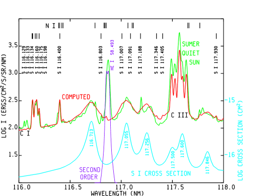
Figure 1: The upper curves show how the calculated disk-center intensity compares with the SUMER observations in the 116 to 118 nm range. The scale on the left gives the intensity, i.e., the spectral radiance. The lower curve is the S i photoionization cross section (right scale) that includes the six autoionization lines.

We also include the 14 lines of N i in this wavelength range having log gf $\geq$ –3.0. The wavelength positions of the N i lines, along with those of S i, are indicated at the top of the figure. The four strongest N i lines are at 116.745, 116.854, 116.389, and 116.433 nm, with log gf values –0.675, –0.817, –1.038, and –1.249, respectively, according to the tables of Wiese et al. (wiese (1996)). The first of these appears on the red side of the 116.713 nm broad emission feature. The second is obscured by the overlapping second-order He i line. The third appears in the blue wing of the S i 116.400 nm emission line. The fourth N i line appears in our calculated spectrum just longward of the S i 116.400 nm line but is not present in the observed spectrum, despite having a strength 0.6 times that of the nearby N i 116.389 nm line from the same multiplet. We cannot explain this discrepancy, but note that the stronger line is blended with the S i line while the weaker one is not. This could be resolved when we have included the effects of blending between S i and N i lines.

We note that while the nitrogen abundance is almost 10 times that of sulfur, the N i lines in this wavelength range are much weaker because their lower energy level is an excited state, and the N i departures from LTE are greater than those of S i.

The narrow emission feature at 117.195 nm is an unidentified line (W. Curdt, private communication), and is not the S I 117.188 nm line, which is too weak to appear. We defer a discussion of other lines and continua to a subsequent paper (Avrett, Fontenla, & Loeser, in preparation, hereafter AFL).

4 Formation of the S i spectrum

We solve the coupled statistical equilibrium and radiative transfer equations for a S i atomic model with 23 energy levels and 111 line transitions. We must specify line strengths, line broadening parameters, collisional excitation and ionization rates, and photoionization cross sections. Few of these values are well known, but we can often determine through experimentation which parameters critically affect the results and which do not. For example, the photoionization cross sections and the collisional ionization rates for the lowest S i levels largely control the S i contribution to the continuum shortward of 120 nm. Emission line strengths are generally sensitive to collisional excitation rates. The S i lines considered here all have upper levels above the S ii threshold and are sensitive to the collisional coupling between these levels and the S ii continuum.

The photoionization rates depend on integrations over a large wavelength range that includes a large number of lines, some strongly in emission. We cannot calculate the spectrum in the 116 to 118 nm region without solving the statistical equilibrium and radiative transfer equations for hydrogen, Si i, C i, and several other constituents in addition to S i. The AFL paper cited above will show results of non-LTE calculations that include H, $\rm{H}^{-}$, He i-ii, C i-iv, N i-iv, O i-vi, Ne i-viii, Na i-ii, Mg i-ii, Al i-ii, Si i-iv, S i-iv, Ca i-ii, and Fe i-ii, applied to the interpretation of the SUMER atlas of Curdt et al. between 67 and 161 nm. Our non-LTE atmospheric modeling calculations use the Pandora computer program of Avrett & Loeser (avrett (2003)).

Our current working model of the low chromosphere is listed in Table 1. This model is similar to the average quiet Sun model C of Vernazza et al. (vernazza (1981)), updated by Fontenla et al. (fontenla (1999)), but we have made adjustments to improve agreement with the observed distribution of brightness temperatures with wavelength in the millimeter range (see Loukitcheva et al. louk (2004)) and with the continuum intensities in the SUMER atlas, including the continuum intensities shown here. This model will be revised further and presented in detail in the AFL paper based on more complete comparisons with SUMER observations.

The table lists, as functions of height (above $\tau_{500\rm{nm}}=1$), the adopted values of the temperature and a broadening velocity $V$. This broadening, or microturbulent, velocity is inferred from observed non-thermal doppler widths of lines formed at various heights, and is used not only for line broadening but also as a turbulent pressure velocity in determining the total hydrogen number density $N_{\rm{H}}$ from hydrostatic equilibrium. The electron number density $N_{\rm{e}}$ is determined from the degree of ionization of the various elements in the calculation.

Table 1: Adopted low chromospheric model for the average quiet Sun

Height(km)	$T$(K)	$V$(km $\rm{s}^{-1}$)	$N_{\rm{H}}(\rm{cm}^{-3})$	$N_{\rm{e}}(\rm{cm}^{-3})$
1750	6785	8.17	4.17E+11	8.38E+10
1660	6750	7.64	6.19E+11	7.62E+10
1580	6710	7.16	8.90E+11	7.48E+10
1500	6670	6.66	1.30E+12	8.00E+10
1420	6615	6.14	1.94E+12	8.83E+10
1340	6540	5.58	2.97E+12	9.63E+10
1270	6420	5.06	4.45E+12	1.01E+11
1180	6200	4.32	7.87E+12	1.01E+11
1080	5840	3.37	1.62E+13	8.00E+10
990	5520	2.61	3.27E+13	6.35E+10
925	5290	2.27	5.56E+13	5.16E+10
860	5080	2.01	9.64E+13	4.37E+10
810	4940	1.77	1.50E+14	4.09E+10
770	4850	1.58	2.14E+14	4.22E+10
720	4750	1.35	3.38E+14	4.92E+10
660	4650	1.09	5.90E+14	6.85E+10

5 Comparison of the broad emission and the continuum

Consider the two wavelengths 116.316 and 116.713 nm. The first is a continuum wavelength relatively free of lines, and the second is centered on the strongest broad emission feature.

Fig. 2 shows, for the two wavelengths, as functions of both height $h$ and monochromatic optical depth $\tau_{\lambda}$: the Planck function $B$ corresponding to the temperatures in Table 1, the continuum source function $S$, the mean intensity $J$, and the function $dI/dh$ that gives the intensity contribution per unit height to the calculated emergent intensity $I$ at disk center ($\mu=1$) and near the limb ($\mu=0.2$). The two emergent intensity values are indicated on the right in both cases. The emission feature has a larger intensity than the continuum because of its larger source funtion.

Since $S$ increases outwards, the formation region occurs at optical depths that are somewhat smaller than unity. The two panels show that the peak intensity contributions occur higher in the atmosphere than $\tau=1$ for the disk-center intensity, or $\tau=0.2$ for the limb intensity at $\mu=0.2$.

In Fig. 3 we show the calculated center-to-limb and off-limb intensities for the two wavelengths. Both show brightening toward the limb, resulting from the outwardly increasing temperature. The intensity in the emission feature has a maximum just at, or inside, the limb, corresponding to the maximum of $S$ in the upper panel of Fig. 2. The continuum intensity is smaller on the disk, and exhibits a sharp increase just at the limb. Above the limb, the calculated intensity in the emission feature extends to greater heights than does the continuum intensity. This is expected, since the opacity in the emission feature is greater than in the continuum.

The limb observations shown by Wilhelm et al. in their Fig. 5 show brightening toward the limb at both wavelengths, with continuum intensities much smaller than those in the emission feature, and a maximum intensity in the emission feature that appears to occur just inside the limb.

The observed intensity in the emission feature above the limb, however, extends further than in our calculation. Their Fig. 6 shows that the separation between the peak intensity of the emission feature just inside the limb and 0.1 times this peak intensity above the limb is about 5” of arc, or about 3600 km, which is much larger than the 2000 km or so in our calculation. This can be interpreted as due to the irregularities in height of the atmospheric layers, which are not accounted for by the assumed spherical symmetry in our calculations.

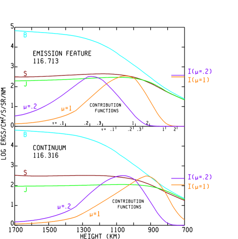
Figure 2: For the two wavelengths 116.316 and 116.713 nm: the variation with $h$ and with $\tau_{\lambda}$ of $B$, $S$, and $J$, and of $dI/dh$ for $\mu=1$ and $\mu=0.2$. The emergent intensity values for $\mu=1$ and $\mu=0.2$ are indicated on the right for each wavelength.

Our calculations also show that the continuum intensity reaches a maximum at a very short distance above the limb, with a maximum value just above the intensity of the emission feature at that location. Their Fig. 5 shows extended patches of continuum emission above the limb that could be due to emission from extended inhomogeneous structures that are not represented in our 1-dimensional modeling. The results in their Fig. 8 and Table 2 indicate that the continuum intensity reaches a maximum just above the limb, as our calculations suggest, but that the continuum emission appears to remain above that of the emission feature at greater heights, contrary to our results. However, Wilhelm (private communication) points out that the SUMER data available in December 2004 did not allow the photospheric limb position to be determined to the accuracy best suited for this comparision.

We have found that the calculated continuum intensity above the limb in this wavelength region is quite sensitive to the departures from LTE in H, S i, Si i, and C i in the higher layers of the atmosphere, i.e., to the effective scattering that we calculate in these layers due to the large number of emission lines overlapping the corresponding continua. We continue to study these effects, particularly the relative importance of scattering and absorption in the many emission lines that affect these photoionization rates. Further center-to-limb observations at various EUV wavelenghts would be very useful for such studies.

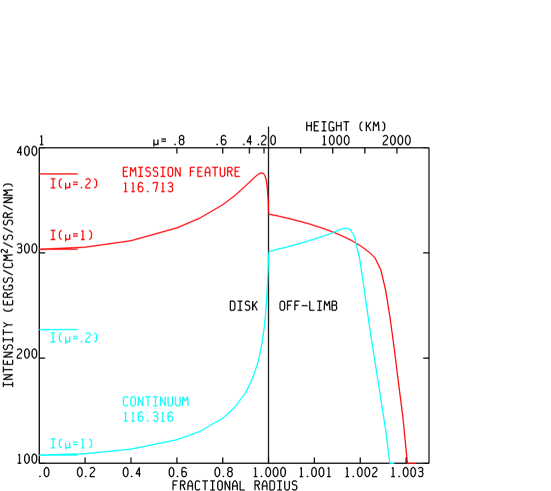
Figure 3: Calculated center-to-limb and off-limb intensity variations at the two wavelengths.

6 Temperature Variations

Finally we show how the calculated intensities are affected by higher and lower model temperatures. We calculate models based on chromospheric temperatures 200 K higher and 200 K lower than in the model listed in Table 1. The two calculated intensity distributions in the 116 to 118 nm range are shown in Fig. 4 along with the same average quiet Sun observations as in Fig. 1. The 200 K changes were introduced at all heights from the temperature minimum region into the transition region. From hydrostatic equilibrium, increasing/decreasing the temperature in the minimum region causes a smaller/larger decrease of $N_{\rm{H}}$ with height in the chromosphere, so that the results in Fig. 4 reflect changes in density as well as temperature. The ratio of intensities corresponding to the temperature changes between –200 K and +200 K is about 4 at the continuum wavelength 116.316 nm, and is about 3 for the emission feature at 116.713 nm.

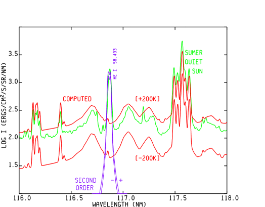
Figure 4: Intensities calculated from a model with chromospheric temperatures 200 K higher and 200 K lower than in Table 1, compared with the SUMER observations of the average quiet Sun.

The SUMER atlas of Curdt et al. gives the observed ratio of bright network to cell interior as a function of wavelength. This ratio appears to be about 1.7 at the center of the strongest autoionization feature, and about 2.0 at the continuum wavelength 116.316 nm. Wilhelm et al. show, in their Fig. 4, the observed variation with time (mainly 3-minute oscillations) of the autoionization emission. The intensity has peak-to-peak variations of about 1.5 in the inter-network, and about 1.3 in network regions.

The calculated range of intensities coresponding to $\pm$ 200 K is much greater than the range of observed quiet-Sun intensity variations: 1) with time, as shown in Fig. 4 of Wilhelm et al., and 2) with position between inter-network and network regions, as shown in the SUMER atlas.

These results show the temperature sensitivity of the calculated intensities. We do not claim to have determined the temperature distribution to within $\pm$ 200 K, since changing some of the important rates and cross sections, and changing the treatment of emission lines involved in photoionization, can have large effects.

7 Conclusions

We have demonstrated that the broad emission features discussed by Wilhelm et al. are the result of S i autoionization transitions. Using a 1-dimensional, time-independent model to represent the chromosphere of the average quiet Sun, we have calculated the spectrum in the 116 to 118 nm band and have shown that the results roughly agree with the disk-center quiet-Sun observations from the SUMER atlas of Curdt et al. Also, our calculated center-to-limb variations are similar to the variations observed by Wilhelm et al. We find that temperature variations of $\pm$ 200 K lead to calculated intensity variations much greater than the temporal and spatial variations observed in quiet solar regions.

With regard to such temperature variations, we note that Carlsson & Stein (carlssonstein (1995)) regard the low chromosphere in Table 1 as wholly dynamic in nature, with temperatures varying by 1000 K or more as individual shocks travel through the atmosphere, and with significant time intervals during which the temperature has no outward increase. The 3D simulations of Wedemeyer et al. (wedemeyer (2004)) support this view that the observed chromospheric emission does not necessarily imply an outward increase in the average gas temperature but can be explained by the presence of substantial spatial and temporal temperature inhomogenities.

However, as pointed out by Carlsson, Judge, & Wilhelm (carlsson (1997)), simulations that do not have a persistent chromospheric temperature rise do not qualitatively reproduce the behavior of the chromospheric emission lines which are observed to be in emission at all times and all locations. A recent discussion of this issue is provided by Fossum & Carlsson fossum (2005).

Given the variation of intensity with temperature shown here, and given the moderate observed intensity fluctuations, both in continua and in lines, we conclude that models having a persistent outward temperature increase, but with moderate temporal and spatial variations, match observations better than current dynamical models that exhibit very large temperature fluctuations. Results for other wavelengths supporting this conclusion will be given in subsequent papers.

- (1) Altun, Z. 1992, J.Phys. B., 25, 2279
- (2) Avrett, E. H., & Loeser, R. 2003, in Modeling of Stellar Atmospheres, IAU Symp. No. 210, ed. W. Weiss & N. Piskunov, Kluwer, Dordrecht, A-21
- (3) Carlsson, M., Judge, P. G., & Wilhelm, K. 1997, ApJL, 486, L63
- (4) Carlsson, M., & Stein, R. F. 1995, ApJ, 440, 29
- (5) Chen, C.-T., & Robicheaux, F. 1994, Phys. Rev. A, 50, 3968
- (6) Curdt, W., Brekke, P., Feldman, U., Wilhelm, K., Dwivedi, B. N., Schühle, U., & Lemaire, P. 2001, A&A, 375, 591
- (7) Fawcett, B. C. 1986, Atomic Data & Nuclear Data Tables, 35, 18
- (8) Fontenla, J. M., White, O. R., Fox, P. A., Avrett, E. H., & Kurucz, R. L. 1999, ApJ, 518, 480
- (9) Fossum, A, & Carlsson, M. 2005, Nature, 435, 919
- (10) Gibson, S.T., Greene, J.P., Ruscic, B., & Berkowitz, J., 1986, J. Phys. B., 19, 2825
- (11) Kurucz, R.L. 2002, in Atomic and Molecular Data and their Applications, ed. D.R. Schultz, P.S. Krstic, & F. Ownby, AIP Conf. Ser. 636, 134
- (12) Loukitcheva, M., Solanki, S. K., Carlsson, M., & Stein, R. F. 2004, A&A 419, 747
- (13) Shore, B. W. 1968, Phys. Rev., 171, 43
- (14) Vernazza, J. E., Avrett, E. H., & Loeser, R. 1981, ApJS, 45, 635
- (15) Wedemeyer, S., Freytag, B., Steffen, M., Ludwig, H. -G., & Holweger, H. 2004, A&A, 414, 1121
- (16) Wiese, W. L., Fuhr, J. R., & Deters T. M. 1996, Atomic Transition Probabilities of Carbon, Nitrogen, and Oxygen, J. Phys. Chem. Ref. Data, Monograph No. 7
- (17) Wilhelm, K., Schühle, U., Curdt, W., Hilchenbach, M., Marsch, E., Lemaire, P., Bertaux, J.-L., Jordan, S. D., & Feldman, U. 2005, A&A, 439, 701