First Light

Abstract

The first dwarf galaxies, which constitute the building blocks of the collapsed objects we find today in the Universe, had formed hundreds of millions of years after the big bang. This pedagogical review describes the early growth of their small-amplitude seed fluctuations from the epoch of inflation through dark matter decoupling and matter-radiation equality, to the final collapse and fragmentation of the dark matter on all mass scales above $\sim 10^{-4}M_{\odot}$. The condensation of baryons into halos in the mass range of $\sim 10^{5}$–$10^{10}M_{\odot}$ led to the formation of the first stars and the re-ionization of the cold hydrogen gas, left over from the big bang. The production of heavy elements by the first stars started the metal enrichment process that eventually led to the formation of rocky planets and life.

A wide variety of instruments currently under design [including large-aperture infrared telescopes on the ground or in space (JWST), and low-frequency arrays for the detection of redshifted 21cm radiation], will establish better understanding of the first sources of light during an epoch in cosmic history that was largely unexplored so far. Numerical simulations of reionization are computationally challenging, as they require radiative transfer across large cosmological volumes as well as sufficently high resolution to identify the sources of the ionizing radiation. The technological challenges for observations and the computational challenges for numerical simulations, will motivate intense work in this field over the coming decade.

Disclaimer: This review was written as an introductory text for a series of lectures at the SAAS-FEE 2006 winter school, and so it includes a limited sample of references on each subject. It does not intend to provide a comprehensive list of all up-to-date references on the topics under discussion, but rather to raise the interest of beginning graduate students in the related literature.

1 Opening Remarks

When I open the daily newspaper as part of my morning routine, I often see lengthy descriptions of conflicts between people on borders, properties, or liberties. Today’s news is often forgotten a few days later. But when one opens ancient texts that have appealed to a broad audience over a longer period of time, such as the Bible, what does one often find in the opening chapter?… a discussion of how the constituents of the Universe (including light, stars and life) were created. Although humans are often occupied with mundane problems, they are curious about the big picture. As citizens of the Universe, we cannot help but wonder how the first sources of light formed, how life came to existence, and whether we are alone as intelligent beings in this vast space. As astronomers in the twenty first century, we are uniquely positioned to answer these big questions with scientific instruments and a quantitative methodology. In this pedagogical review, intended for students preparing to specialize in cosmology, I will describe current ideas about one of these topics: the appearance of the first sources of light and their influence on the surrounding Universe. This topic is one of the most active frontiers in present-day cosmology. As such it is an excellent area for a PhD thesis of a graduate student interested in cosmology. I will therefore highlight the unsolved questions in this field as much as the bits we understand.

2 Excavating the Universe for Clues About Its History

When we look at our image reflected off a mirror at a distance of 1 meter, we see the way we looked 6 nano-seconds ago, the light travel time to the mirror and back. If the mirror is spaced $10^{19}~{}{\rm cm}=3$pc away, we will see the way we looked twenty one years ago. Light propagates at a finite speed, and so by observing distant regions, we are able to see how the Universe looked like in the past, a light travel time ago. The statistical homogeneity of the Universe on large scales guarantees that what we see far away is a fair statistical representation of the conditions that were present in in our region of the Universe a long time ago.

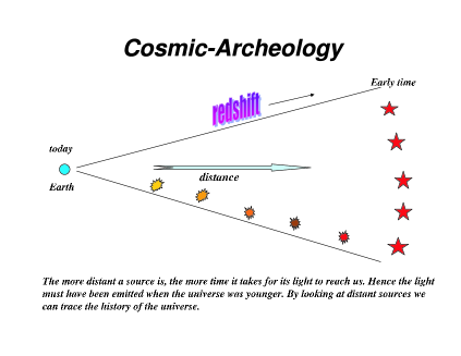
Figure 1: Cosmology is like archeology. The deeper one looks, the older is the layer that one is revealing, owing to the finite propagation speed of light.

This fortunate situation makes cosmology an empirical science. We do not need to guess how the Universe evolved. Using telescopes we can simply see the way it appeared at earlier cosmic times. Since a greater distance means a fainter flux from a source of a fixed luminosity, the observation of the earliest sources of light requires the development of sensitive instruments and poses challenges to observers.

We can in principle image the Universe only if it is transparent. Earlier than 0.4 million years after the big bang, the cosmic plasma was ionized and the Universe was opaque to Thomson scattering by the dense gas of free electrons that filled it. Thus, telescopes cannot be used to image the infant Universe at earlier times (or redshifts $>10^{3}$). The earliest possible image of the Universe was recorded by COBE and WMAP (see Fig. 2).

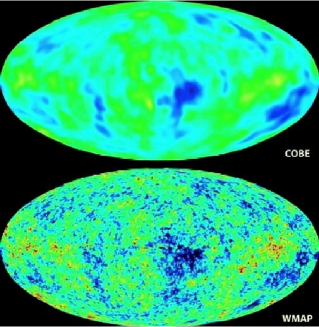
Figure 2: Images of the Universe shortly after it became transparent, taken by the COBE and WMAP satellites (see http://map.gsfc.nasa.gov/ for details). The slight density inhomogeneties in the otherwise uniform Universe, imprinted hot and cold brightness map of the cosmic microwave background. The existence of these anisotropies was predicted three decades before the technology for taking this image became available in a number of theoretical papers, including zel ; sachs ; sciama ; silk ; peeb .

Figure 3: The optical depth of the Universe to electron scattering (upper panel) and the ionization fraction (lower panel) as a function of redshift before reionization. Observatories of electromagnetic radiation cannot image the opaque Universe beyond a redshift of $z\sim 1100$.

3 Bakground Cosmological Model

3.1 The Expanding Universe

The modern physical description of the Universe as a whole can be traced back to Einstein, who argued theoretically for the so-called “cosmological principle”: that the distribution of matter and energy must be homogeneous and isotropic on the largest scales. Today isotropy is well established (see the review by Wu, Lahav, & Rees 1999 Wu99 ) for the distribution of faint radio sources, optically-selected galaxies, the X-ray background, and most importantly the cosmic microwave background (hereafter, CMB; see, e.g., Bennett et al. 1996 Be96 ). The constraints on homogeneity are less strict, but a cosmological model in which the Universe is isotropic but significantly inhomogeneous in spherical shells around our special location, is also excluded Goodman95 .

In General Relativity, the metric for a space which is spatially homogeneous and isotropic is the Friedman-Robertson-Walker metric, which can be written in the form

$$ds^{2}=dt^{2}-a^{2}(t)\left[\frac{dR^{2}}{1-k\,R^{2}}+R^{2}\left(d\theta^{2}+\sin^{2}\theta\,d\phi^{2}\right)\right]\ ,$$ (1)

where $a(t)$ is the cosmic scale factor which describes expansion in time, and $(R,\theta,\phi)$ are spherical comoving coordinates. The constant $k$ determines the geometry of the metric; it is positive in a closed Universe, zero in a flat Universe, and negative in an open Universe. Observers at rest remain at rest, at fixed $(R,\theta,\phi)$, with their physical separation increasing with time in proportion to $a(t)$. A given observer sees a nearby observer at physical distance $D$ receding at the Hubble velocity $H(t)D$, where the Hubble constant at time $t$ is $H(t)=d\,a(t)/dt$. Light emitted by a source at time $t$ is observed at $t=0$ with a redshift $z=1/a(t)-1$, where we set $a(t=0)\equiv 1$ for convenience (but note that old textbooks may use a different convention).

The Einstein field equations of General Relativity yield the Friedmann equation (e.g., Weinberg 1972 We72 ; Kolb & Turner 1990 Kolb90 )

$$H^{2}(t)=\frac{8\pi G}{3}\rho-\frac{k}{a^{2}}\ ,$$ (2)

which relates the expansion of the Universe to its matter-energy content. For each component of the energy density $\rho$, with an equation of state $p=p(\rho)$, the density $\rho$ varies with $a(t)$ according to the equation of energy conservation

$$d(\rho R^{3})=-pd(R^{3})\ .$$ (3)

With the critical density

$$\rho_{C}(t)\equiv\frac{3H^{2}(t)}{8\pi G}$$ (4)

defined as the density needed for $k=0$, we define the ratio of the total density to the critical density as

$$\Omega\equiv\frac{\rho}{\rho_{C}}\ .$$ (5)

With ${\Omega_{m}}$, ${\Omega_{\Lambda}}$, and ${\Omega_{r}}$ denoting the present contributions to $\Omega$ from matter (including cold dark matter as well as a contribution $\Omega_{b}$ from baryons), vacuum density (cosmological constant), and radiation, respectively, the Friedmann equation becomes

$$\frac{H(t)}{H_{0}}=\left[\frac{{\Omega_{m}}}{a^{3}}+{\Omega_{\Lambda}}+\frac{{\Omega_{r}}}{a^{4}}+\frac{{\Omega_{k}}}{a^{2}}\right]\ ,$$ (6)

where we define $H_{0}$ and $\Omega_{0}={\Omega_{m}}+{\Omega_{\Lambda}}+{\Omega_{r}}$ to be the present values of $H$ and $\Omega$, respectively, and we let

$${\Omega_{k}}\equiv-\frac{k}{H_{0}^{2}}=1-\Omega_{m}.$$ (7)

In the particularly simple Einstein-de Sitter model (${\Omega_{m}}=1$, ${\Omega_{\Lambda}}={\Omega_{r}}={\Omega_{k}}=0$), the scale factor varies as $a(t)\propto t^{2/3}$. Even models with non-zero ${\Omega_{\Lambda}}$ or ${\Omega_{k}}$ approach the Einstein-de Sitter behavior at high redshift, i.e. when $(1+z)\gg|{\Omega_{m}}^{-1}-1|$ (as long as ${\Omega_{r}}$ can be neglected). In this high-$z$ regime the age of the Universe is,

$$t\approx{2\over 3H_{0}\sqrt{\Omega_{m}}}\left(1+z\right)^{-3/2}~{}.$$ (8)

The Friedmann equation implies that models with ${\Omega_{k}}=0$ converge to the Einstein-de Sitter limit faster than do open models.

In the standard hot Big Bang model, the Universe is initially hot and the energy density is dominated by radiation. The transition to matter domination occurs at $z\sim 3500$, but the Universe remains hot enough that the gas is ionized, and electron-photon scattering effectively couples the matter and radiation. At $z\sim 1100$ the temperature drops below $\sim 3000$K and protons and electrons recombine to form neutral hydrogen. The photons then decouple and travel freely until the present, when they are observed as the CMB WMAP .

3.2 Composition of the Universe

According to the standard cosmological model, the Universe started at the big bang about 14 billion years ago. During an early epoch of accelerated superluminal expansion, called inflation, a region of microscopic size was stretched to a scale much bigger than the visible Universe and our local geometry became flat. At the same time, primordial density fluctuations were generated out of quantum mechanical fluctuations of the vacuum. These inhomogeneities seeded the formation of present-day structure through the process of gravitational instability. The mass density of ordinary (baryonic) matter makes up only a fifth of the matter that led to the emergence of structure and the rest is the form of an unknown dark matter component. Recently, the Universe entered a new phase of accelerated expansion due to the dominance of some dark vacuum energy density over the ever rarefying matter density.

The basic question that cosmology attempts to answer is:

What are the ingredients (composition and initial conditions) of the Universe and what processes generated the observed structures in it?

In detail, we would like to know:

(a) Did inflation occur and when? If so, what drove it and how did it end?

(b) What is the nature of of the dark energy and how does it change over time and space?

(c) What is the nature of the dark matter and how did it regulate the evolution of structure in the Universe?

Before hydrogen recombined, the Universe was opaque to electromagnetic radiation, precluding any possibility for direct imaging of its evolution. The only way to probe inflation is through the fossil record that it left behind in the form of density perturbations and gravitational waves. Following inflation, the Universe went through several other milestones which left a detectable record. These include: baryogenesis (which resulted in the observed asymmetry between matter and anti-matter), the electroweak phase transition (during which the symmetry between electromagnetic and weak interactions was broken), the QCD phase transition (during which protons and neutrons were assembled out of quarks and gluons), the dark matter freeze-out epoch (during which the dark matter decoupled from the cosmic plasma), neutrino decoupling, electron-positron annihilation, and light-element nucleosynthesis (during which helium, deuterium and lithium were synthesized). The signatures that these processes left in the Universe can be used to constrain its parameters and answer the above questions.

Half a million years after the big bang, hydrogen recombined and the Universe became transparent. The ultimate goal of observational cosmology is to image the entire history of the Universe since then. Currently, we have a snapshot of the Universe at recombination from the CMB, and detailed images of its evolution starting from an age of a billion years until the present time. The evolution between a million and a billion years has not been imaged as of yet.

Within the next decade, NASA plans to launch an infrared space telescope (JWST) that will image the very first sources of light (stars and black holes) in the Universe, which are predicted theoretically to have formed in the first hundreds of millions of years. In parallel, there are several initiatives to construct large-aperture infrared telescopes on the ground with the same goal in mind^{, ,}. The neutral hydrogen, relic from cosmological recombination, can be mapped in three-dimensions through its 21cm line even before the first galaxies formed Loeb04 . Several groups are currently constructing low-frequency radio arrays in an attempt to map the initial inhomogeneities as well as the process by which the hydrogen was re-ionized by the first galaxies.

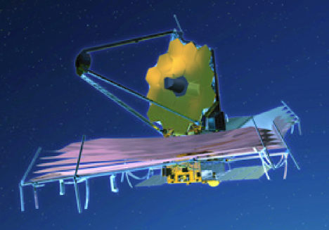
Figure 4: A sketch of the current design for the James Webb Space Telescope, the successor to the Hubble Space Telescope to be launched in 2011 (http://www.jwst.nasa.gov/). The current design includes a primary mirror made of beryllium which is 6.5 meter in diameter as well as an instrument sensitivity that spans the full range of infrared wavelengths of 0.6–28$\mu$m and will allow detection of the first galaxies in the infant Universe. The telescope will orbit 1.5 million km from Earth at the Lagrange L2 point.

The next generation of ground-based telescopes will have a diameter of twenty to thirty meter. Together with JWST (that will not be affected by the atmospheric backgound) they will be able to image the first galaxies. Given that these galaxies also created the ionized bubbles around them, the same galaxy locations should correlate with bubbles in the neutral hydrogen (created by their UV emission). Within a decade it would be possible to explore the environmental influence of individual galaxies by using the two sets of instruments in concert WyBar .

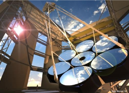
Figure 5: Artist conception of the design for one of the future giant telescopes that could probe the first generation of galaxies from the ground. The Giant Magellan Telescope (GMT) will contain seven mirrors (each 8.4 meter in diameter) and will have the resolving power equivalent to a 24.5 meter (80 foot) primary mirror. For more details see http://www.gmto.org/

The dark ingredients of the Universe can only be probed indirectly through a variety of luminous tracers. The distribution and nature of the dark matter are constrained by detailed X-ray and optical observations of galaxies and galaxy clusters. The evolution of the dark energy with cosmic time will be constrained over the coming decade by surveys of Type Ia supernovae, as well as surveys of X-ray clusters, up to a redshift of two.

On large scales ($>10$Mpc) the power-spectrum of primordial density perturbations is already known from the measured microwave background anisotropies, galaxy surveys, weak lensing, and the Ly$\alpha$ forest. Future programs will refine current knowledge, and will search for additional trademarks of inflation, such as gravitational waves (through CMB polarization), small-scale structure (through high-redshift galaxy surveys and 21cm studies), or the Gaussian statistics of the initial perturbations.

The big bang is the only known event where particles with energies approaching the Planck scale [$(\hbar c^{5}/G)^{1/2}\sim 10^{19}~{}{\rm GeV}$] interacted. It therefore offers prospects for probing the unification physics between quantum mechanics and general relativity (to which string theory is the most-popular candidate). Unfortunately, the exponential expansion of the Universe during inflation erases memory of earlier cosmic epochs, such as the Planck time.

3.3 Linear Gravitational Growth

Observations of the CMB (e.g., Bennett et al. 1996 Be96 ) show that the Universe at recombination was extremely uniform, but with spatial fluctuations in the energy density and gravitational potential of roughly one part in $10^{5}$. Such small fluctuations, generated in the early Universe, grow over time due to gravitational instability, and eventually lead to the formation of galaxies and the large-scale structure observed in the present Universe.

As before, we distinguish between fixed and comoving coordinates. Using vector notation, the fixed coordinate ${\bf r}$ corresponds to a comoving position ${\bf x}={\bf r}/a$. In a homogeneous Universe with density $\rho$, we describe the cosmological expansion in terms of an ideal pressureless fluid of particles each of which is at fixed ${\bf x}$, expanding with the Hubble flow ${\bf v}=H(t){\bf r}$ where ${\bf v}=d{\bf r}/dt$. Onto this uniform expansion we impose small perturbations, given by a relative density perturbation

$$\delta({\bf x})=\frac{\rho({\bf r})}{\bar{\rho}}-1\ ,$$ (9)

where the mean fluid density is $\bar{\rho}$, with a corresponding peculiar velocity ${\bf u}\equiv{\bf v}-H{\bf r}$. Then the fluid is described by the continuity and Euler equations in comoving coordinates p80 ; Peebles :

$$\frac{\partial\delta}{\partial t}+\frac{1}{a}{\bf\nabla}\cdot\left[(1+\delta){\bf u}\right] = 0$$ (10)

$$\frac{\partial{\bf u}}{\partial t}+H{\bf u}+\frac{1}{a}({\bf u}\cdot{\bf\nabla}){\bf u} = -\frac{1}{a}{\bf\nabla}\phi\ .$$ (11)

The potential $\phi$ is given by the Poisson equation, in terms of the density perturbation:

$$\nabla^{2}\phi=4\pi G\bar{\rho}a^{2}\delta\ .$$ (12)

This fluid description is valid for describing the evolution of collisionless cold dark matter particles until different particle streams cross. This “shell-crossing” typically occurs only after perturbations have grown to become non-linear, and at that point the individual particle trajectories must in general be followed. Similarly, baryons can be described as a pressureless fluid as long as their temperature is negligibly small, but non-linear collapse leads to the formation of shocks in the gas.

For small perturbations $\delta\ll 1$, the fluid equations can be linearized and combined to yield

$$\frac{\partial^{2}\delta}{\partial t^{2}}+2H\frac{\partial\delta}{\partial t}=4\pi G\bar{\rho}\delta\ .$$ (13)

This linear equation has in general two independent solutions, only one of which grows with time. Starting with random initial conditions, this “growing mode” comes to dominate the density evolution. Thus, until it becomes non-linear, the density perturbation maintains its shape in comoving coordinates and grows in proportion to a growth factor $D(t)$. The growth factor in the matter-dominated era is given by p80

$$D(t)\propto\frac{\left({\Omega_{\Lambda}}a^{3}+{\Omega_{k}}a+{\Omega_{m}}\right)^{1/2}}{a^{3/2}}\int_{0}^{a}\frac{a^{\prime 3/2}\,da^{\prime}}{\left({\Omega_{\Lambda}}a^{\prime 3}+{\Omega_{k}}a^{\prime}+{\Omega_{m}}\right)^{3/2}}\ ,$$ (14)

where we neglect ${\Omega_{r}}$ when considering halos forming in the matter-dominated regime at $z\ll 10^{4}$. In the Einstein-de Sitter model (or, at high redshift, in other models as well) the growth factor is simply proportional to $a(t)$.

The spatial form of the initial density fluctuations can be described in Fourier space, in terms of Fourier components

$$\delta_{\bf k}=\int d^{3}x\,\delta(x)e^{-i{\bf k}\cdot{\bf x}}\ .$$ (15)

Here we use the comoving wavevector ${\bf k}$, whose magnitude $k$ is the comoving wavenumber which is equal to $2\pi$ divided by the wavelength. The Fourier description is particularly simple for fluctuations generated by inflation (e.g., Kolb & Turner 1990 Kolb90 ). Inflation generates perturbations given by a Gaussian random field, in which different ${\bf k}$-modes are statistically independent, each with a random phase. The statistical properties of the fluctuations are determined by the variance of the different ${\bf k}$-modes, and the variance is described in terms of the power spectrum $P(k)$ as follows:

$$\left<\delta_{{\bf k}}\delta_{{\bf k^{\prime}}}^{*}\right>=\left(2\pi\right)^{3}P(k)\,\delta^{(3)}\left({\bf k}-{\bf k^{\prime}}\right)\ ,$$ (16)

where $\delta^{(3)}$ is the three-dimensional Dirac delta function. The gravitational potential fluctuations are sourced by the density fluctuations through Poisson’s equation.

In standard models, inflation produces a primordial power-law spectrum $P(k)\propto k^{n}$ with $n\sim 1$. Perturbation growth in the radiation-dominated and then matter-dominated Universe results in a modified final power spectrum, characterized by a turnover at a scale of order the horizon $cH^{-1}$ at matter-radiation equality, and a small-scale asymptotic shape of $P(k)\propto k^{n-4}$. The overall amplitude of the power spectrum is not specified by current models of inflation, and it is usually set by comparing to the observed CMB temperature fluctuations or to local measures of large-scale structure.

Since density fluctuations may exist on all scales, in order to determine the formation of objects of a given size or mass it is useful to consider the statistical distribution of the smoothed density field. Using a window function $W({\bf r})$ normalized so that $\int d^{3}r\,W({\bf r})=1$, the smoothed density perturbation field, $\int d^{3}r\delta({\bf x})W({\bf r})$, itself follows a Gaussian distribution with zero mean. For the particular choice of a spherical top-hat, in which $W=1$ in a sphere of radius $R$ and is zero outside, the smoothed perturbation field measures the fluctuations in the mass in spheres of radius $R$. The normalization of the present power spectrum is often specified by the value of $\sigma_{8}\equiv\sigma(R=8h^{-1}{\rm Mpc})$. For the top-hat, the smoothed perturbation field is denoted $\delta_{R}$ or $\delta_{M}$, where the mass $M$ is related to the comoving radius $R$ by $M=4\pi\rho_{m}R^{3}/3$, in terms of the current mean density of matter $\rho_{m}$. The variance $\langle\delta_{M}\rangle^{2}$ is

$$\sigma^{2}(M)=\sigma^{2}(R)=\int_{0}^{\infty}\frac{dk}{2\pi^{2}}\,k^{2}P(k)\left[\frac{3j_{1}(kR)}{kR}\right]^{2}\ ,$$ (17)

where $j_{1}(x)=(\sin x-x\cos x)/x^{2}$. The function $\sigma(M)$ plays a crucial role in estimates of the abundance of collapsed objects, as we describe later.

Species that decouple from the cosmic plasma (like the dark matter or the baryons) would show fossil evidence for acoustic oscillations in their power spectrum of inhomogeneities due to sound waves in the radiation fluid to which they were coupled at early times. This phenomenon can be understood as follows. Imagine a localized point-like perturbation from inflation at $t=0$. The small perturbation in density or pressure will send out a sound wave that will reach the sound horizon $c_{s}t$ at any later time $t$. The perturbation will therefore correlate with its surroundings up to the sound horizon and all $k$-modes with wavelengths equal to this scale or its harmonics will be correlated. The scales of the perturbations that grow to become the first collapsed objects at $z<100$ cross the horizon in the radiation dominated era after the dark matter decouples from the cosmic plasma. Next we consider the imprint of this decoupling on the smallest-scale structure of the dark matter.

3.4 The Smallest-Scale Power Spectrum of Cold Dark Matter

A broad range of observational data involving the dynamics of galaxies, the growth of large-scale structure, and the dynamics and nucleosynthesis of the Universe as a whole, indicate the existence of dark matter with a mean cosmic mass density that is $\sim 5$ times larger than the density of the baryonic matter Jungman ; WMAP . The data is consistent with a dark matter composed of weakly-interacting, massive particles, that decoupled early and adiabatically cooled to an extremely low temperature by the present time Jungman . The Cold Dark Matter (CDM) has not been observed directly as of yet, although laboratory searches for particles from the dark halo of our own Milky-Way galaxy have been able to restrict the allowed parameter space for these particles. Since an alternative more-radical interpretation of the dark matter phenomenology involves a modification of gravity Beken , it is of prime importance to find direct fingerprints of the CDM particles. One such fingerprint involves the small-scale structure in the Universe Green , on which we focus in this section.

The most popular candidate for the CDM particle is a Weakly Interacting Massive Particle (WIMP). The lightest supersymmetric particle (LSP) could be a WIMP (for a review see Jungman ). The CDM particle mass depends on free parameters in the particle physics model but typical values cover a range around $M\sim 100~{}{\rm GeV}$ (up to values close to a TeV). In many cases the LSP hypothesis will be tested at the Large Hadron Collider (e.g. battaglia ) or in direct detection experiments (e.g. baltz ).

The properties of the CDM particles affect their response to the small-scale primordial inhomogeneities produced during cosmic inflation. The particle cross-section for scattering off standard model fermions sets the epoch of their thermal and kinematic decoupling from the cosmic plasma (which is significantly later than the time when their abundance freezes-out at a temperature $T\sim M$). Thermal decoupling is defined as the time when the temperature of the CDM stops following that of the cosmic plasma while kinematic decoupling is defined as the time when the bulk motion of the two species start to differ. For CDM the epochs of thermal and kinetic decoupling coincide. They occur when the time it takes for collisions to change the momentum of the CDM particles equals the Hubble time. The particle mass determines the thermal spread in the speeds of CDM particles, which tends to smooth-out fluctuations on very small scales due to the free-streaming of particles after kinematic decoupling Green ; Green2 . Viscosity has a similar effect before the CDM fluid decouples from the cosmic radiation fluid Hofmann . An important effect involves the memory the CDM fluid has of the acoustic oscillations of the cosmic radiation fluid out of which it decoupled. Here we consider the imprint of these acoustic oscillations on the small-scale power spectrum of density fluctuations in the Universe. Analogous imprints of acoustic oscillations of the baryons were identified recently in maps of the CMB WMAP , and the distribution of nearby galaxies Eisenste ; these signatures appear on much larger scales, since the baryons decouple much later when the scale of the horizon is larger. The discussion in this section follows Loeb & Zaldarriaga (2005) Loe05 .

Formalism

Kinematic decoupling of CDM occurs during the radiation-dominated era. For example, if the CDM is made of neutralinos with a particle mass of $\sim 100~{}{\rm GeV}$, then kinematic decoupling occurs at a cosmic temperature of $T_{\rm d}\sim 10~{}{\rm MeV}$ Hofmann ; Chen . As long as $T_{d}\ll 100~{}{\rm MeV}$, we may ignore the imprint of the QCD phase transition (which transformed the cosmic quark-gluon soup into protons and neutrons) on the CDM power spectrum Schmid . Over a short period of time during this transition, the pressure does not depend on density and the sound speed of the plasma vanishes, resulting in a significant growth for perturbations with periods shorter than the length of time over which the sound speed vanishes. The transition occurs when the temperature of the cosmic plasma is $\sim 100-200~{}{\rm MeV}$ and lasts for a small fraction of the Hubble time. As a result, the induced modifications are on scales smaller than those we are considering here and the imprint of the QCD phase transition is washed-out by the effects we calculate.

At early times the contribution of the dark matter to the energy density is negligible. Only at relatively late times when the cosmic temperature drops to values as low as $\sim 1$ eV, matter and radiation have comparable energy densities. As a result, the dynamics of the plasma at earlier times is virtually unaffected by the presence of the dark matter particles. In this limit, the dynamics of the radiation determines the gravitational potential and the dark matter just responds to that potential. We will use this simplification to obtain analytic estimates for the behavior of the dark matter transfer function.

The primordial inflationary fluctuations lead to acoustic modes in the radiation fluid during this era. The interaction rate of the particles in the plasma is so high that we can consider the plasma as a perfect fluid down to a comoving scale,

$$\lambda_{f}\sim\eta_{d}/\sqrt{N}\ \ \ \ ;\ \ \ N\sim n\sigma t_{d},$$ (18)

where $\eta_{d}=\int_{0}^{t_{d}}dt/a(t)$ is the conformal time (i.e. the comoving size of the horizon) at the time of CDM decoupling, $t_{d}$; $\sigma$ is the scattering cross section and $n$ is the relevant particle density. (Throughout this section we set the speed of light and Planck’s constant to unity for brevity.) The damping scale depends on the species being considered and its contribution to the energy density, and is the largest for neutrinos which are only coupled through weak interactions. In that case $N\sim(T/T_{d}^{\nu})^{3}$ where $T_{d}^{\nu}\sim 1\ {\rm MeV}$ is the temperature of neutrino decoupling. At the time of CDM decoupling $N\sim M/T_{d}\sim 10^{4}$ for the rest of the plasma, where $M$ is the mass of the CDM particle. Here we will consider modes of wavelength larger than $\lambda_{f}$, and so we neglect the effect of radiation diffusion damping and treat the plasma (without the CDM) as a perfect fluid.

The equations of motion for a perfect fluid during the radiation era can be solved analytically. We will use that solution here, following the notation of Dodelson Dodelson . As usual we Fourier decompose fluctuations and study the behavior of each Fourier component separately. For a mode of comoving wavenumber $k$ in Newtonian gauge, the gravitational potential fluctuations are given by:

$$\Phi=3\Phi_{p}\left[{\sin(\omega\eta)-\omega\eta\cos(\omega\eta)\over(\omega\eta)^{3}}\right],$$ (19)

where $\omega=k/\sqrt{3}$ is the frequency of a mode and $\Phi_{p}$ is its primordial amplitude in the limit $\eta\rightarrow 0$. In this section we use conformal time $\eta=\int dt/a(t)$ with $a(t)\propto t^{1/2}$ during the radiation-dominated era. Expanding the temperature anisotropy in multipole moments and using the Boltzmann equation to describe their evolution, the monopole $\Theta_{0}$ and dipole $\Theta_{1}$ of the photon distribution can be written in terms of the gravitational potential as Dodelson :

$$\Theta_{0} = \Phi\left({x^{2}\over 6}+{1\over 2}\right)+{x\over 2}\Phi^{\prime}$$

$$\Theta_{1} = -{x^{2}\over 6}\left(\Phi^{\prime}+{1\over x}\Phi\right)$$ (20)

where $x\equiv k\eta$ and a prime denotes a derivative with respect to $x$.

The solutions in equations (19) and (20) assume that both the sound speed and the number of relativistic degrees of freedom are constant over time. As a result of the QCD phase transition and of various particles becoming non-relativistic, both of these assumptions are not strictly correct. The vanishing sound speed during the QCD phase transition provides the most dramatic effect, but its imprint is on scales smaller than the ones we consider here because the transition occurs at a significantly higher temperature and only lasts for a fraction of the Hubble time Schmid .

Before the dark matter decouples kinematically, we will treat it as a fluid which can exchange momentum with the plasma through particle collisions. At early times, the CDM fluid follows the motion of the plasma and is involved in its acoustic oscillations. The continuity and momentum equations for the CDM can be written as:

$$\dot{\delta}_{c}+\theta_{c} = 3\dot{\Phi}$$

$$\dot{\theta}_{c}+{\dot{a}\over a}\theta_{c} = k^{2}c_{s}^{2}\delta_{c}-k^{2}\sigma_{c}-k^{2}\Phi+\tau_{c}^{-1}(\Theta_{1}-\theta_{c})$$ (21)

where a dot denotes an $\eta$-derivative, $\delta_{c}$ is the dark matter density perturbation, $\theta_{c}$ is the divergence of the dark matter velocity field and $\sigma_{c}$ denotes the anisotropic stress. In writing these equations we have followed Ref. Ma . The term $\tau_{c}^{-1}(\Theta_{1}-\theta_{c})$ encodes the transfer of momentun between the radiation and CDM fluids and $\tau_{c}^{-1}$ provides the collisional rate of momentum transfer,

$$\tau_{c}^{-1}=n\sigma{T\over M}a,$$ (22)

with $n$ being the number density of particles with which the dark matter is interacting, $\sigma(T)$ the average cross section for interaction and $M$ the mass of the dark matter particle. The relevant scattering partners are the standard model leptons which have thermal abundances. For detailed expressions of the cross section in the case of supersymmetric (SUSY) dark matter, see Refs. Chen ; Green2 . For our purpose, it is sufficient to specify the typical size of the cross section and its scaling with cosmic time,

$$\sigma\approx{T^{2}\over M_{\sigma}^{4}},$$ (23)

where the coupling mass $M_{\sigma}$ is of the order of the weak-interaction scale ($\sim 100$ GeV) for SUSY dark matter. This equation should be taken as the definition of $M_{\sigma}$, as it encodes all the uncertainties in the details of the particle physics model into a single parameter. The temperature dependance of the averaged cross section is a result of the available phase space. Our results are quite insensitive to the details other than through the decoupling time. Equating $\tau_{c}^{-1}/a$ to the Hubble expansion rate gives the temperature of kinematic decoupling:

$$T_{d}=\left({M_{\sigma}^{4}M\over M_{pl}}\right)^{1/4}\approx 10\ {\rm MeV}\left({M_{\sigma}\over 100\ {\rm GeV}}\right)\left(M\over 100\ {\rm GeV}\right)^{1/4}.$$ (24)

The term $k^{2}c_{s}^{2}\delta_{c}$ in Eq. (21) results from the pressure gradient force and $c_{s}$ is the dark matter sound speed. In the tight coupling limit, $\tau_{c}\ll H^{-1}$ we find that $c_{s}^{2}\approx f_{c}T/M$ and that the shear term is $k^{2}\sigma_{c}\approx f_{v}c_{s}^{2}\tau_{c}\theta_{c}$. Here $f_{v}$ and $f_{c}$ are constant factors of order unity. We will find that both these terms make a small difference on the scales of interest, so their precise value is unimportant.

By combining both equations in (21) into a single equation for $\delta_{c}$ we get

$$\delta_{c}^{\prime\prime} + {1\over x}\left[1+F_{\rm v}(x)\right]\delta_{c}^{\prime}+c_{s}^{2}(x)\delta_{c}$$

$$= S(x) -3F_{\rm v}(x)\Phi^{\prime}+{x_{d}^{4}\over x^{5}}\left(3\theta_{0}^{\prime}-\delta_{c}^{\prime}\right),$$ (25)

where $x_{d}=k\eta_{d}$ and $\eta_{d}$ denotes the time of kinematic decoupling which can be expressed in terms of the decoupling temperature as,

$$\eta_{d}={2t_{d}(1+z_{d})}\approx{M_{pl}\over T_{0}T_{d}} \approx 10\ {\rm pc}\ \left({T_{d}\over 10\ {\rm MeV}}\right)^{-1}$$ (26)

$$\propto M_{\sigma}^{-1}M^{-1/4},$$

with $T_{0}=2.7$K being the present-day CMB temperature and $z_{d}$ being the redshift at kinematic decoupling. We have also introduced the source function,

$$S(x)\equiv-3\Phi^{\prime\prime}+\Phi-{3\over x}\Phi^{\prime}.$$ (27)

For $x\ll x_{d}$, the dark matter sound speed is given by

$$c_{s}^{2}(x)=c_{s}^{2}(x_{d}){x_{d}\over x},$$ (28)

where $c_{s}^{2}(x_{d})$ is the dark matter sound speed at kinematic decoupling (in units of the speed of light),

$$c_{s}(x_{d})\approx 10^{-2}f_{c}^{1/2}\left({T_{d}\over 10\ {\rm MeV}}\right)^{1/2}\left({M\over 100\ {\rm GeV}}\right)^{-1/2}.$$ (29)

In writing (28) we have assumed that prior to decoupling the temperature of the dark matter follows that of the plasma. For the viscosity term we have,

$$F_{v}(x)=f_{v}c_{s}^{2}(x_{d})x_{d}^{2}\left({x_{d}\over x}\right)^{5}.$$ (30)

Free streaming after kinematic decoupling

In the limit of the collision rate being much slower than the Hubble expansion, the CDM is decoupled and the evolution of its perturbations is obtained by solving a Boltzman equation:

$${\partial f\over\partial\eta}+{dr_{i}\over d\eta}{\partial f\over\partial r_{i}}+{dq_{i}\over d\eta}{\partial f\over\partial q_{i}}=0,$$ (31)

where $f(\vec{r},\vec{q},\eta)$ is the distribution function which depends on position, comoving momentum $\vec{q}$, and time. The comoving momentum 3-components are ${dx_{i}/d\eta}=q_{i}/a$. We use the Boltzman equation to find the evolution of modes that are well inside the horizon with $x\gg 1$. In the radiation era, the gravitational potential decays after horizon crossing (see Eq. 19). In this limit the comoving momentum remains constant, ${dq_{i}/d\eta}=0$ and the Boltzman equation becomes,

$${\partial f\over\partial\eta}+{q_{i}\over a}{\partial f\over\partial r_{i}}=0.$$ (32)

We consider a single Fourier mode and write $f$ as,

$$f(\vec{r},\vec{q},\eta)=f_{0}(q)[1+\delta_{F}(\vec{q},\eta)e^{i\vec{k}\cdot\vec{r}}],$$ (33)

where $f_{0}(q)$ is the unperturbed distribution,

$$f_{0}(q)=n_{\rm CDM}\left({M\over 2\pi T_{\rm CDM}}\right)^{3/2}\exp\left[-{1\over 2}{Mq^{2}\over T_{\rm CDM}}\right]$$ (34)

where $n_{\rm CDM}$ and $T_{\rm CDM}$ are the present-day density and temperature of the dark matter.

Our approach is to solve the Boltzman equation with initial conditions given by the fluid solution at a time $\eta_{*}$ (which will depend on $k$). The simplified Boltzman equation can be easily solved to give $\delta_{F}(\vec{q},\eta)$ as a function of the initial conditions $\delta_{F}(\vec{q},\eta_{*})$,

$$\delta_{F}(\vec{q},\eta)=\delta_{F}(\vec{q},\eta_{*})\exp[-i\vec{q}\cdot\vec{k}{\eta_{*}\over a(\eta_{*})}\ln(\eta/\eta_{*})].$$ (35)

The CDM overdensity $\delta_{c}$ can then be expressed in terms of the perturbation in the distribution function as,

$$\delta_{c}(\eta)={1\over n_{\rm CDM}}\int d^{3}q\ f_{0}(q)\ \delta_{F}(\vec{q},\eta).$$ (36)

We can use (35) to obtain the evolution of $\delta_{c}$ in terms of its value at $\eta_{*}$,

$$\delta_{c}(\eta)=\exp\left[-{1\over 2}{k^{2}\over k_{f}^{2}}\ln^{2}({\eta\over\eta_{*}})\right]\ \left[\delta|_{\eta_{*}}+{d\delta\over d\eta}|_{\eta_{*}}\eta_{*}\ln({\eta\over\eta_{*}})\right],$$ (37)

where $k_{f}^{-2}=\sqrt{(T_{d}/M)}\eta_{d}$. The exponential term is responsible for the damping of perturbations as a result of free streaming and the dispersion of the CDM particles after they decouple from the plasma. The above expression is only valid during the radiation era. The free streaming scale is simply given by $\int dt(v/a)\propto\int dta^{-2}$ which grows logarithmically during the radiation era as in equation (37) but stops growing in the matter era when $a\propto t^{2/3}$.

Equation (37) can be used to show that even during the free streaming epoch, $\delta_{c}$ satisfies equation (25) but with a modified sound speed and viscous term. For $x\gg x_{d}$ one should use,

$$c_{s}^{2}(x) = c_{s}^{2}(x_{d})\left({x_{d}\over x}\right)^{2}\left[1+x_{d}^{2}c_{s}^{2}(x_{d})\ln^{2}({x\over x_{d}})\right]$$

$$F_{v}(x) = 2c_{s}^{2}(x_{d})x_{d}^{2}\ln\left({x_{d}\over x}\right)$$ (38)

The differences between the above scalings and those during the tight coupling regime are a result of the fact that the dark matter temperature stops following the plasma temperature but rather scales as $a^{-2}$ after thermal decoupling, which coincides with the kinematic decoupling. We ignore the effects of heat transfer during the fluid stage of the CDM because its temperature is controlled by the much larger heat reservoir of the radiation-dominated plasma at that stage.

To obtain the transfer function we solve the dark matter fluid equation until decoupling and then evolve the overdensity using equation (37) up to the time of matter–radiation equality. In practice, we use the fluid equations up to $x_{*}=10\ {\rm max}(x_{d},10)$ so as to switch into the free streaming solution well after the gravitational potential has decayed. In the fluid equations, we smoothly match the sound speed and viscosity terms at $x=x_{d}$. As mentioned earlier, because $c_{s}(x_{d})$ is so small and we are interested in modes that are comparable to the size of the horizon at decoupling, i.e. $x_{d}\sim{\rm few}$, both the dark matter sound speed and the associated viscosity play only a minor role, and our simplified treatment is adequate.

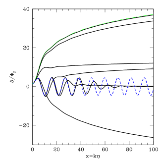
Figure 6: The normalized amplitude of CDM fluctuations $\delta/\Phi_{P}$ for a variety of modes with comoving wavenumbers $\log(k\eta_{d})=(0,1/3,2/3,1,4/3,5/3,2)$ as a function of $x\equiv k\eta$, where $\eta=\int_{0}^{t}dt/a(t)$ is the conformal time coordinate. The dashed line shows the temperature monopole $3\theta_{0}$ and the uppermost (dotted) curve shows the evolution of a mode that is uncoupled to the cosmic plasma.

In Figure 6 we illustrate the time evolution of modes during decoupling for a variety of $k$ values. The situation is clear. Modes that enter the horizon before kinematic decoupling oscillate with the radiation fluid. This behavior has two important effects. In the absence of the coupling, modes receive a “kick” by the source term $S(x)$ as they cross the horizon. After that they grow logarithmically. In our case, modes that entered the horizon before kinematic decoupling follow the plasma oscillations and thus miss out on both the horizon “kick” and the beginning of the logarithmic growth. Second, the decoupling from the radiation fluid is not instantaneous and this acts to further damp the amplitude of modes with $x_{d}\gg 1$. This effect can be understood as follows. Once the oscillation frequency of the mode becomes high compared to the scattering rate, the coupling to the plasma effectively damps the mode. In that limit one can replace the forcing term $\Theta_{0}^{\prime}$ by its average value, which is close to zero. Thus in this regime, the scattering is forcing the amplitude of the dark matter oscillations to zero. After kinematic decoupling the modes again grow logarithmically but from a very reduced amplitude. The coupling with the plasma induces both oscillations and damping of modes that entered the horizon before kinematic decoupling. This damping is different from the free streaming damping that occurs after kinematic decoupling.

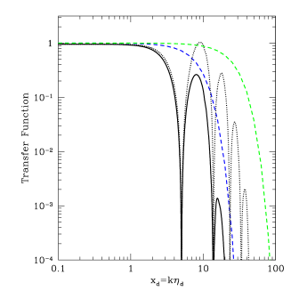
Figure 7: Transfer function of the CDM density perturbation amplitude (normalized by the primordial amplitude from inflation). We show two cases: (i) $T_{d}/M=10^{-4}$ and $T_{d}/T_{\rm eq}=10^{7}$; (ii) $T_{d}/M=10^{-5}$ and $T_{d}/T_{\rm eq}=10^{7}$. In each case the oscillatory curve is our result and the other curve is the free-streaming only result that was derived previously in the literature [4,7,8].

In Figure 7 we show the resulting transfer function of the CDM overdensity. The transfer function is defined as the ratio between the CDM density perturbation amplitude $\delta_{c}$ when the effect of the coupling to the plasma is included and the same quantity in a model where the CDM is a perfect fluid down to arbitrarily small scales (thus, the power spectrum is obtained by multiplying the standard result by the square of the transfer function). This function shows both the oscillations and the damping signature mentioned above. The peaks occur at multipoles of the horizon scale at decoupling,

$$k_{peak}=(8,15.7,24.7,..)\eta_{d}^{-1}\propto{M_{pl}\over T_{0}T_{d}}.$$ (39)

This same scale determines the “oscillation” damping. The free streaming damping scale is,

$$\eta_{d}c_{d}(\eta_{d})\ln(\eta_{eq}/\eta_{d})\propto{M_{pl}M^{1/2}\over T_{0}T_{d}^{3/2}}\ln(T_{d}/T_{\rm eq}),$$ (40)

where $T_{\rm eq}$ is the temperature at matter radiation equality, $T_{\rm eq}\approx 1\ {\rm eV}$. The free streaming scale is parametrically different from the “oscillation” damping scale. However for our fiducial choice of parameters for the CDM particle they roughly coincide.

The CDM damping scale is significantly smaller than the scales observed directly in the Cosmic Microwave Background or through large scale structure surveys. For example, the ratio of the damping scale to the scale that entered the horizon at Matter-radiation equality is $\eta_{d}/\eta_{eq}\sim T_{eq}/T_{d}\sim 10^{-7}$ and to our present horizon $\eta_{d}/\eta_{0}\sim(T_{eq}T_{0})^{1/2}/T_{d}\sim 10^{-9}$. In the context of inflation, these scales were created 16 and 20 e–folds apart. Given the large extrapolation, one could certainly imagine that a change in the spectrum could alter the shape of the power spectrum around the damping scale. However, for smooth inflaton potentials with small departures from scale invariance this is not likely to be the case. On scales much smaller than the horizon at matter radiation equality, the spectrum of perturbations density before the effects of the damping are included is approximately,

$$\Delta^{2}(k) \propto \exp\left[(n-1)\ln(k\eta_{eq})+{1\over 2}\alpha^{2}\ln(k\eta_{eq})^{2}+\cdots\right]$$ (41)

$$\times\ln^{2}(k\eta_{eq}/8)$$

where the first term encodes the shape of the primordial spectrum and the second the transfer function. Primordial departures from scale invariance are encoded in the slope $n$ and its running $\alpha$. The effective slope at scale $k$ is then,

$${\partial\ln\Delta^{2}\over\partial\ln k}=(n-1)+\alpha\ln(k\eta_{eq})+{2\over\ln(k\eta_{eq}/8)}.$$ (42)

For typical values of $(n-1)\sim 1/60$ and $\alpha\sim 1/60^{2}$ the slope is still positive at $k\sim\eta_{d}^{-1}$, so the cut-off in the power will come from the effects we calculate rather than from the shape of the primordial spectrum. However given the large extrapolation in scale, one should keep in mind the possibility of significant effects resulting from the mechanisms that generates the density perturbations.

Implications We have found that acoustic oscillations, a relic from the epoch when the dark matter coupled to the cosmic radiation fluid, truncate the CDM power spectrum on a comoving scale larger than effects considered before, such as free-streaming and viscosity Green ; Green2 ; Hofmann . For SUSY dark matter, the minimum mass of dark matter clumps that form in the Universe is therefore increased by more than an order of magnitude to a value of

$$M_{\rm cut} = {4\pi\over 3}\left({\pi\over k_{\rm cut}}\right)^{3}\Omega_{M}\rho_{\rm crit}$$ (43)

$$\simeq 10^{-4}\left({T_{d}\over 10~{}{\rm MeV}}\right)^{-3}M_{\odot},$$

where $\rho_{\rm crit}=(H_{0}^{2}/8\pi G)=9\times 10^{-30}~{}{\rm g~{}cm^{-3}}$ is the critical density today, and $\Omega_{M}$ is the matter density for the concordance cosmological model WMAP . We define the cut-off wavenumber $k_{\rm cut}$ as the point where the transfer function first drops to a fraction $1/e$ of its value at $k\rightarrow 0$. This corresponds to $k_{\rm cut}\approx 3.3\ \eta_{d}^{-1}$.

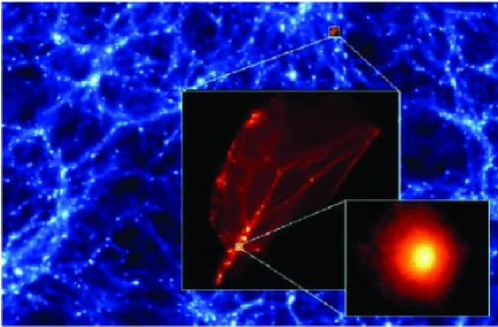
Figure 8: A slice through a numerical simulation of the first dark matter condensations to form in the Universe. Colors represent the dark matter density at $z=26$. The simulated volume is 60 comoving pc on a side, simulated with 64 million particles each weighing $1.2\times 10^{-10}M_{\odot}$ (!). (from Diemand, Moore, & Stadel 2005 Moore ).

Recent numerical simulations Moore ; Gao of the earliest and smallest objects to have formed in the Universe (see Fig. 8), need to be redone for the modified power spectrum that we calculated in this section. Although it is difficult to forecast the effects of the acoustic oscillations through the standard Press-Schechter formalism Press , it is likely that the results of such simulations will be qualitatively the same as before except that the smallest clumps would have a mass larger than before (as given by Eq. 43).

Potentially, there are several observational signatures of the smallest CDM clumps. As pointed out in the literature Moore ; Stoehr , the smallest CDM clumps could produce $\gamma$-rays through dark-matter annihilation in their inner density cusps, with a flux in excess of that from nearby dwarf galaxies. If a substantial fraction of the Milky Way halo is composed of CDM clumps with a mass $\sim 10^{-4}M_{\odot}$, the nearest clump is expected to be at a distance of $\sim 4\times 10^{17}$ cm. Given that the characteristic speed of such clumps is a few hundred ${\rm km~{}s^{-1}}$, the $\gamma$-ray flux would therefore show temporal variations on the relatively long timescale of a thousand years. Passage of clumps through the solar system should also induce fluctuations in the detection rate of CDM particles in direct search experiments. Other observational effects have rather limited prospects for detectability. Because of their relatively low-mass and large size ($\sim 10^{17}~{}{\rm cm}$), the CDM clumps are too diffuse to produce any gravitational lensing signatures (including femto-lensing Gould ), even at cosmological distances.

The smallest CDM clumps should not affect the intergalactic baryons which have a much larger Jeans mass. However, once objects above $\sim 10^{6}M_{\odot}$ start to collapse at redshifts $z<30$, the baryons would be able to cool inside of them via molecular hydrogen transitions and the interior baryonic Jeans mass would drop. The existence of dark matter clumps could then seed the formation of the first stars inside these objects Bromm .

3.5 Structure of the Baryons

Early Evolution of Baryonic Perturbations on Large Scales

The baryons are coupled through Thomson scattering to the radiation fluid until they become neutral and decouple. After cosmic recombination, they start to fall into the potential wells of the dark matter and their early evolution was derived by Barkana & Loeb (2005) BLinf .

On large scales, the dark matter (dm) and the baryons (b) are affected only by their combined gravity and gas pressure can be ignored. The evolution of sub-horizon linear perturbations is described in the matter-dominated regime by two coupled second-order differential equations Peebles :

$$\ddot{\delta}_{\rm dm}+2H\dot{\delta}_{\rm dm} = 4\pi G\bar{\rho}_{m}\left(f_{\rm b}\delta_{\rm b}+f_{\rm dm}\delta_{\rm dm}\right)\ ,$$

$$\ddot{\delta}_{\rm b}+2H\dot{\delta}_{\rm b} = 4\pi G\bar{\rho}_{m}\left(f_{\rm b}\delta_{\rm b}+f_{\rm dm}\delta_{\rm dm}\right)\ ,$$ (44)

where $\delta_{\rm dm}(t)$ and $\delta_{\rm b}(t)$ are the perturbations in the dark matter and baryons, respectively, the derivatives are with respect to cosmic time $t$, $H(t)=\dot{a}/a$ is the Hubble constant with $a=(1+z)^{-1}$, and we assume that the mean mass density $\bar{\rho}_{m}(t)$ is made up of respective mass fractions $f_{\rm dm}$ and $f_{\rm b}=1-f_{\rm dm}$. Since these linear equations contain no spatial gradients, they can be solved spatially for $\delta_{\rm dm}({\bf x},t)$ and $\delta_{\rm b}({\bf x},t)$ or in Fourier space for ${\tilde{\delta}}_{\rm dm}({\bf k},t)$ and ${\tilde{\delta}}_{\rm b}({\bf k},t)$.

Defining $\delta_{\rm tot}\equiv f_{\rm b}\delta_{\rm b}+f_{\rm dm}\delta_{\rm dm}$ and $\delta_{\rm b-}\equiv\delta_{\rm b}-\delta_{\rm tot}$ , we find

$$\ddot{\delta}_{\rm tot}+2H\dot{\delta}_{\rm tot} = 4\pi G\bar{\rho}_{m}\delta_{\rm tot}\ ,$$

$$\ddot{\delta}_{\rm b-}+2H\dot{\delta}_{\rm b-} = 0\ .$$ (45)

Each of these equations has two independent solutions. The equation for $\delta_{\rm tot}$ has the usual growing and decaying solutions, which we denote $D_{1}(t)$ and $D_{4}(t)$, respectively, while the $\delta_{\rm b-}$ equation has solutions $D_{2}(t)$ and $D_{3}(t)$; we number the solutions in order of declining growth rate (or increasing decay rate). We assume an Einstein-de Sitter, matter-dominated Universe in the redshift range $z=20$–150, since the radiation contributes less than a few percent at $z<150$, while the cosmological constant and the curvature contribute to the energy density less than a few percent at $z>3$. In this regime $a\propto t^{2/3}$ and the solutions are $D_{1}(t)=a/a_{i}$ and $D_{4}(t)=(a/a_{i})^{-3/2}$ for $\delta_{\rm tot}$, and $D_{2}(t)=1$ and $D_{3}(t)=(a/a_{i})^{-1/2}$ for $\delta_{\rm b-}$, where we have normalized each solution to unity at the starting scale factor $a_{i}$, which we set at a redshift $z_{i}=150$. The observable baryon perturbation can then be written as

$${\tilde{\delta}}_{\rm b}({\bf k},t)={\tilde{\delta}}_{\rm b-}+{\tilde{\delta}}_{\rm tot}=\sum_{m=1}^{4}{\tilde{\delta}}_{m}({\bf k})\,D_{m}(t)\ ,$$ (46)

and similarly for the dark matter perturbation,

$${\tilde{\delta}}_{\rm dm}={1\over f_{\rm dm}}\left({\tilde{\delta}}_{\rm tot}-f_{b}{\tilde{\delta}}_{b}\right)=\sum_{m=1}^{4}{\tilde{\delta}}_{m}({\bf k})\,C_{m}(t)\ ,$$ (47)

where $C_{i}=D_{i}$ for $i=1,4$ and $C_{i}=-(f_{\rm b}/f_{\rm dm})D_{i}$ for $i=2,3$. We may establish the values of ${\tilde{\delta}}_{m}({\bf k})$ by inverting the $4\times 4$ matrix ${\bf A}$ that relates the 4-vector $({\tilde{\delta}}_{1},{\tilde{\delta}}_{2},{\tilde{\delta}}_{3},{\tilde{\delta}}_{4})$ to the 4-vector that represents the initial conditions $({\tilde{\delta}}_{\rm b},{\tilde{\delta}}_{\rm dm},\dot{{\tilde{\delta}}}_{\rm b},\dot{{\tilde{\delta}}}_{\rm dm})$ at the initial time.

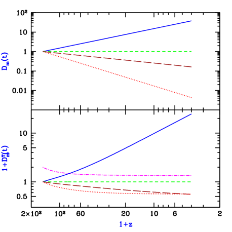
Figure 9: Redshift evolution of the amplitudes of the independent modes of the density perturbations (upper panel) and the temperature perturbations (lower panel), starting at redshift 150 (from Barkana & Loeb 2005 BLinf ). We show $m=1$ (solid curves), $m=2$ (short-dashed curves), $m=3$ (long-dashed curves), $m=4$ (dotted curves), and $m=0$ (dot-dashed curve). Note that the lower panel shows one plus the mode amplitude.

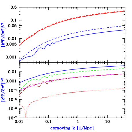
Figure 10: Power spectra and initial perturbation amplitudes versus wavenumber (from BLinf ). The upper panel shows ${\tilde{\delta}}_{\rm b}$ (solid curves) and ${\tilde{\delta}}_{\rm dm}$ (dashed curves) at $z=150$ and 20 (from bottom to top). The lower panel shows the initial ($z=150$) amplitudes of ${\tilde{\delta}}_{1}$ (solid curve), ${\tilde{\delta}}_{2}$ (short-dashed curve), ${\tilde{\delta}}_{3}$ (long-dashed curve), ${\tilde{\delta}}_{4}$ (dotted curve), and ${\tilde{\delta}}_{T}(t_{i})$ (dot-dashed curve). Note that if ${\tilde{\delta}}_{1}$ is positive then so are ${\tilde{\delta}}_{3}$ and ${\tilde{\delta}}_{T}(t_{i})$, while ${\tilde{\delta}}_{2}$ is negative at all $k$, and ${\tilde{\delta}}_{4}$ is negative at the lowest $k$ but is positive at $k>0.017$ Mpc^-1.

Next we describe the fluctuations in the sound speed of the cosmic gas caused by Compton heating of the gas, which is due to scattering of the residual electrons with the CMB photons. The evolution of the temperature $T$ of a gas element of density $\rho_{b}$ is given by the first law of thermodynamics:

$$dQ=\frac{3}{2}kdT-kTd\log\rho_{\rm b}\ ,$$ (48)

where $dQ$ is the heating rate per particle. Before the first galaxies formed,

$$\frac{dQ}{dt}=4\frac{\sigma_{\rm T}\,c}{m_{e}}\,k(T_{\gamma}-T)\rho_{\gamma}x_{e}(t)\ ,$$ (49)

where $\sigma_{T}$ is the Thomson cross-section, $x_{e}(t)$ is the electron fraction out of the total number density of gas particles, and $\rho_{\gamma}$ is the CMB energy density at a temperature $T_{\gamma}$. In the redshift range of interest, we assume that the photon temperature ($T_{\gamma}=T_{\gamma}^{0}/a$) is spatially uniform, since the high sound speed of the photons (i.e., $c/\sqrt{3}$) suppresses fluctuations on the sub-horizon scales that we consider, and the horizon-scale $\sim 10^{-5}$ fluctuations imprinted at cosmic recombination are also negligible compared to the smallWe establish the values of ${\tilde{\delta}}_{m}({\bf k})$ by inverting the $4\times 4$ matrix ${\bf A}$ that relates the 4-vector $({\tilde{\delta}}_{1},{\tilde{\delta}}_{2},{\tilde{\delta}}_{3},{\tilde{\delta}}_{4})$ to the 4-vector that represents the initial conditions $({\tilde{\delta}}_{\rm b},{\tilde{\delta}}_{\rm dm},\dot{{\tilde{\delta}}}_{\rm b},\dot{{\tilde{\delta}}}_{\rm dm})$ at the initial time. er-scale fluctuations in the gas density and temperature. Fluctuations in the residual electron fraction $x_{e}(t)$ are even smaller. Thus,

$$\frac{dT}{dt}=\frac{2}{3}T\frac{d\log\rho_{\rm b}}{dt}+\frac{x_{e}(t)}{t_{\gamma}}\,(T_{\gamma}-T)\,a^{-4}\ ,$$ (50)

where $t_{\gamma}^{-1}\equiv\bar{\rho}_{\gamma}^{0}({8\sigma_{\rm T}\,c}/{3m_{e}})=8.55\times 10^{-13}{\rm yr}^{-1}$. After cosmic recombination, $x_{e}(t)$ changes due to the slow recombination rate of the residual ions:

$${dx_{e}(t)\over dt}=-\alpha_{B}(T)x_{e}^{2}(t)\bar{n}_{H}(1+y)\ ,$$ (51)

where $\alpha_{B}(T)$ is the case-B recombination coefficient of hydrogen, $\bar{n}_{H}$ is the mean number density of hydrogen at time $t$, and $y=0.079$ is the helium to hydrogen number density ratio. This yields the evolution of the mean temperature, ${d\bar{T}}/{dt}=-2H\bar{T}+{x_{e}(t)}{t_{\gamma}^{-1}}\,(T_{\gamma}-\bar{T})\,a^{-4}$. In prior analyses Peebles ; Ma a spatially uniform speed of sound was assumed for the gas at each redshift. Note that we refer to $\delta p/\delta\rho$ as the square of the sound speed of the fluid, where $\delta p$ is the pressure perturbation, although we are analyzing perturbations driven by gravity rather than sound waves driven by pressure gradients.

Instead of assuming a uniform sound speed, we find the first-order perturbation equation,

$$\frac{d\delta_{T}}{dt}=\frac{2}{3}\frac{d\delta_{b}}{dt}-\frac{x_{e}(t)}{t_{\gamma}}\frac{T_{\gamma}}{\bar{T}}a^{-4}\delta_{T}\ ,$$ (52)

where we defined the fractional temperature perturbation $\delta_{T}$. Like the density perturbation equations, this equation can be solved separately at each ${\bf x}$ or at each ${\bf k}$. Furthermore, the solution $\delta_{T}(t)$ is a linear functional of $\delta_{b}(t)$ [for a fixed function $x_{e}(t)$]. Thus, if we choose an initial time $t_{i}$ then using Eq. (46) we can write the solution in Fourier space as

$${\tilde{\delta}}_{T}({\bf k},t)=\sum_{m=1}^{4}{\tilde{\delta}}_{m}({\bf k})\,D^{T}_{m}(t)+{\tilde{\delta}}_{T}({\bf k},t_{i})\,D^{T}_{0}(t)\ ,$$ (53)

where $D^{T}_{m}(t)$ is the solution of Eq. (52) with $\delta_{T}=0$ at $t_{i}$ and with the perturbation mode $D_{m}(t)$ substituted for $\delta_{b}(t)$, while $D^{T}_{0}(t)$ is the solution with no perturbation $\delta_{b}(t)$ and with $\delta_{T}=1$ at $t_{i}$. By modifying the CMBFAST code (http://www.cmbfast.org/), we can numerically solve Eq. (52) along with the density perturbation equations for each ${\bf k}$ down to $z_{i}=150$, and then match the solution to the form of Eq. (53).

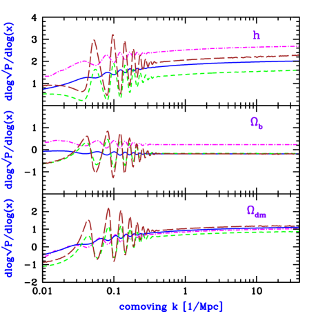
Figure 11: Relative sensitivity of perturbation amplitudes at $z=150$ to cosmological parameters (from BLinf ). For variations in a parameter $x$, we show $d{\rm log}\sqrt{P(k)}/d{\rm log}(x)$. We consider variations in $\Omega_{\rm dm}h^{2}$ (upper panel), in $\Omega_{b}h^{2}$ (middle panel), and in the Hubble constant $h$ (lower panel). When we vary each parameter we fix the other two, and the variations are all carried out in a flat $\Omega_{\rm total}=1$ universe. We show the sensitivity of ${\tilde{\delta}}_{1}$ (solid curves), ${\tilde{\delta}}_{2}$ (short-dashed curves), ${\tilde{\delta}}_{3}$ (long-dashed curves), and ${\tilde{\delta}}_{T}(t_{i})$ (dot-dashed curves).

Figure 9 shows the time evolution of the various independent modes that make up the perturbations of density and temperature, starting at the time $t_{i}$ corresponding to $z_{i}=150$. $D^{T}_{2}(t)$ is identically zero since $D_{2}(t)=1$ is constant, while $D^{T}_{3}(t)$ and $D^{T}_{4}(t)$ are negative. Figure 10 shows the amplitudes of the various components of the initial perturbations. We consider comoving wavevectors $k$ in the range 0.01 – 40 Mpc^-1, where the lower limit is set by considering sub-horizon scales at $z=150$ for which photon perturbations are negligible compared to $\delta_{\rm dm}$ and $\delta_{\rm b}$, and the upper limit is set by requiring baryonic pressure to be negligible compared to gravity. ${\tilde{\delta}}_{2}$ and ${\tilde{\delta}}_{3}$ clearly show a strong signature of the large-scale baryonic oscillations, left over from the era of the photon-baryon fluid before recombination, while ${\tilde{\delta}}_{1}$, ${\tilde{\delta}}_{4}$, and ${\tilde{\delta}}_{T}$ carry only a weak sign of the oscillations. For each quantity, the plot shows $[k^{3}P(k)/(2\pi^{2})]^{1/2}$, where $P(k)$ is the corresponding power spectrum of fluctuations. ${\tilde{\delta}}_{4}$ is already a very small correction at $z=150$ and declines quickly at lower redshift, but the other three modes all contribute significantly to ${\tilde{\delta}}_{\rm b}$, and the ${\tilde{\delta}}_{T}(t_{i})$ term remains significant in ${\tilde{\delta}}_{T}(t)$ even at $z<100$. Note that at $z=150$ the temperature perturbation ${\tilde{\delta}}_{T}$ has a different shape with respect to $k$ than the baryon perturbation ${\tilde{\delta}}_{\rm b}$, showing that their ratio cannot be described by a scale-independent speed of sound.

The power spectra of the various perturbation modes and of ${\tilde{\delta}}_{T}(t_{i})$ depend on the initial power spectrum of density fluctuations from inflation and on the values of the fundamental cosmological parameters ($\Omega_{\rm dm}$, $\Omega_{b}$, $\Omega_{\Lambda}$, and $h$). If these independent power spectra can be measured through 21cm fluctuations, this will probe the basic cosmological parameters through multiple combinations, allowing consistency checks that can be used to verify the adiabatic nature and the expected history of the perturbations. Figure 11 illustrates the relative sensitivity of $\sqrt{P(k)}$ to variations in $\Omega_{\rm dm}h^{2}$, $\Omega_{b}h^{2}$, and $h$, for the quantities ${\tilde{\delta}}_{1}$, ${\tilde{\delta}}_{2}$, ${\tilde{\delta}}_{3}$, and ${\tilde{\delta}}_{T}(t_{i})$. Not shown is ${\tilde{\delta}}_{4}$, which although it is more sensitive (changing by order unity due to $10\%$ variations in the parameters), its magnitude always remains much smaller than the other modes, making it much harder to detect. Note that although the angular scale of the baryon oscillations constrains also the history of dark energy through the angular diameter distance, we have focused here on other cosmological parameters, since the contribution of dark energy relative to matter becomes negligible at high redshift.

Cosmological Jeans Mass

The Jeans length $\lambda_{\rm J}$ was originally defined (Jeans 1928 Jeans28 ) in Newtonian gravity as the critical wavelength that separates oscillatory and exponentially-growing density perturbations in an infinite, uniform, and stationary distribution of gas. On scales $\ell$ smaller than $\lambda_{\rm J}$, the sound crossing time, $\ell/c_{s}$ is shorter than the gravitational free-fall time, $(G\rho)^{-1/2}$, allowing the build-up of a pressure force that counteracts gravity. On larger scales, the pressure gradient force is too slow to react to a build-up of the attractive gravitational force. The Jeans mass is defined as the mass within a sphere of radius $\lambda_{\rm J}/2$, $M_{\rm J}=(4\pi/3)\rho(\lambda_{\rm J}/2)^{3}$. In a perturbation with a mass greater than $M_{\rm J}$, the self-gravity cannot be supported by the pressure gradient, and so the gas is unstable to gravitational collapse. The Newtonian derivation of the Jeans instability suffers from a conceptual inconsistency, as the unperturbed gravitational force of the uniform background must induce bulk motions (compare to Binney & Tremaine 1987 Bi87 ). However, this inconsistency is remedied when the analysis is done in an expanding Universe.

The perturbative derivation of the Jeans instability criterion can be carried out in a cosmological setting by considering a sinusoidal perturbation superposed on a uniformly expanding background. Here, as in the Newtonian limit, there is a critical wavelength $\lambda_{\rm J}$ that separates oscillatory and growing modes. Although the expansion of the background slows down the exponential growth of the amplitude to a power-law growth, the fundamental concept of a minimum mass that can collapse at any given time remains the same (see, e.g. Kolb & Turner 1990 Kolb90 ; Peebles 1993 Peebles ).

We consider a mixture of dark matter and baryons with density parameters $\Omega_{\rm dm}^{\,z}=\bar{\rho}_{\rm dm}/\rho_{\rm c}$ and $\Omega_{\rm b}^{\,z}=\bar{\rho}_{\rm b}/\rho_{\rm c}$, where $\bar{\rho}_{\rm dm}$ is the average dark matter density, $\bar{\rho}_{\rm b}$ is the average baryonic density, $\rho_{\rm c}$ is the critical density, and $\Omega_{\rm dm}^{\,z}+\Omega_{\rm b}^{\,z}={\Omega_{m}^{\,z}}$ is given by equation(89). We also assume spatial fluctuations in the gas and dark matter densities with the form of a single spherical Fourier mode on a scale much smaller than the horizon,

$$\frac{\rho_{\rm dm}(r,t)-\bar{\rho}_{\rm dm}(t)}{\bar{\rho}_{\rm dm}(t)} = \delta_{\rm dm}(t)\frac{\sin(kr)}{kr}\ ,$$ (54)

$$\frac{\rho_{\rm b}(r,t)-\bar{\rho}_{\rm b}(t)}{\bar{\rho}_{\rm b}(t)} = \delta_{\rm b}(t)\frac{\sin(kr)}{kr}\ ,$$ (55)

where $\bar{\rho}_{\rm dm}(t)$ and $\bar{\rho}_{\rm b}(t)$ are the background densities of the dark matter and baryons, $\delta_{\rm dm}(t)$ and $\delta_{\rm b}(t)$ are the dark matter and baryon overdensity amplitudes, $r$ is the comoving radial coordinate, and $k$ is the comoving perturbation wavenumber. We adopt an ideal gas equation-of-state for the baryons with a specific heat ratio $\gamma$=$5/3$. Initially, at time $t=t_{\rm i}$, the gas temperature is uniform $T_{\rm b}(r,t_{\rm i})$=$T_{\rm i}$, and the perturbation amplitudes are small $\delta_{\rm dm,i},\delta_{\rm b,i}\ll 1$. We define the region inside the first zero of $\sin(kr)/(kr)$, namely $0<kr<\pi$, as the collapsing “object”.

The evolution of the temperature of the baryons $T_{\rm b}(r,t)$ in the linear regime is determined by the coupling of their free electrons to the CMB through Compton scattering, and by the adiabatic expansion of the gas. Hence, $T_{\rm b}(r,t)$ is generally somewhere between the CMB temperature, $T_{\gamma}\propto(1+z)^{-1}$ and the adiabatically-scaled temperature $T_{\rm ad}\propto(1+z)^{-2}$. In the limit of tight coupling to $T_{\gamma}$, the gas temperature remains uniform. On the other hand, in the adiabatic limit, the temperature develops a gradient according to the relation

$$T_{\rm b}\propto\rho_{b}^{(\gamma-1)}.$$ (56)

The evolution of a cold dark matter overdensity, $\delta_{\rm dm}(t)$, in the linear regime is described by the equation (44),

$${\ddot{\delta}}_{\rm dm}+2H{\dot{\delta}}_{\rm dm}={3\over 2}H^{2}\left(\Omega_{\rm b}\delta_{\rm b}+\Omega_{\rm dm}\delta_{\rm dm}\right)$$ (57)

whereas the evolution of the overdensity of the baryons, $\delta_{\rm b}(t)$, with the inclusion of their pressure force is described by (see §9.3.2 of Kolb90 ),

$${\ddot{\delta}}_{\rm b}+2H{\dot{\delta}}_{\rm b}={3\over 2}H^{2}\left(\Omega_{\rm b}\delta_{\rm b}+\Omega_{\rm dm}\delta_{\rm dm}\right)-\frac{kT_{\rm i}}{\mu m_{p}}\left({k\over a}\right)^{2}\left(\frac{a_{\rm i}}{a}\right)^{(1+\beta)}\left(\delta_{\rm b}+{2\over 3}\beta[\delta_{\rm b}-\delta_{\rm b,i}]\right).$$ (58)

Here, $H(t)={\dot{a}}/a$ is the Hubble parameter at a cosmological time $t$, and $\mu=1.22$ is the mean molecular weight of the neutral primordial gas in atomic units. The parameter $\beta$ distinguishes between the two limits for the evolution of the gas temperature. In the adiabatic limit $\beta=1$, and when the baryon temperature is uniform and locked to the background radiation, $\beta=0$. The last term on the right hand side (in square brackets) takes into account the extra pressure gradient force in $\nabla(\rho_{\rm b}T)=(T\nabla\rho_{\rm b}+\rho_{\rm b}\nabla T)$, arising from the temperature gradient which develops in the adiabatic limit. The Jeans wavelength $\lambda_{\rm J}=2\pi/k_{\rm J}$ is obtained by setting the right-hand side of equation (58) to zero, and solving for the critical wavenumber $k_{\rm J}$. As can be seen from equation (58), the critical wavelength $\lambda_{\rm J}$ (and therefore the mass $M_{\rm J}$) is in general time-dependent. We infer from equation (58) that as time proceeds, perturbations with increasingly smaller initial wavelengths stop oscillating and start to grow.

To estimate the Jeans wavelength, we equate the right-hand-side of equation (58) to zero. We further approximate $\delta_{\rm b}\sim\delta_{\rm dm}$, and consider sufficiently high redshifts at which the Universe is matter dominated and flat, $(1+z)\gg{\rm max}[(1-\Omega_{m}-\Omega_{\Lambda})/\Omega_{m},(\Omega_{\Lambda}/\Omega_{m})^{1/3}]$. In this regime, $\Omega_{\rm b}\ll{\Omega_{m}}\approx 1$, $H\approx 2/(3t)$, and $a=(1+z)^{-1}\approx(3H_{0}{\sqrt{\Omega_{m}}}/2)^{2/3}t^{2/3}$, where $\Omega_{m}=\Omega_{\rm dm}+\Omega_{b}$ is the total matter density parameter. Following cosmological recombination at $z\approx 10^{3}$, the residual ionization of the cosmic gas keeps its temperature locked to the CMB temperature (via Compton scattering) down to a redshift of Peebles

$$1+z_{t}\approx 160(\Omega_{b}h^{2}/0.022)^{2/5}\ .$$ (59)

In the redshift range between recombination and $z_{t}$, $\beta=0$ and

$$k_{\rm J}\equiv(2\pi/\lambda_{\rm J})=[2kT_{\gamma}(0)/3\mu m_{p}]^{-1/2}{\sqrt{\Omega_{m}}}H_{0}\ ,$$ (60)

so that the Jeans mass is therefore redshift independent and obtains the value (for the total mass of baryons and dark matter)

$$M_{\rm J}\equiv{4\pi\over 3}\left({\lambda_{\rm J}\over 2}\right)^{3}{\bar{\rho}}(0)=1.35\times 10^{5}\left({\Omega_{m}h^{2}\over 0.15}\right)^{-1/2}M_{\odot}\ .$$ (61)

Based on the similarity of $M_{\rm J}$ to the mass of a globular cluster, Peebles & Dicke (1968) Pe68 suggested that globular clusters form as the first generation of baryonic objects shortly after cosmological recombination. Peebles & Dicke assumed a baryonic Universe, with a nonlinear fluctuation amplitude on small scales at $z\sim 10^{3}$, a model which has by now been ruled out. The lack of a dominant mass of dark matter inside globular clusters makes it unlikely that they formed through direct cosmological collapse, and more likely that they resulted from fragmentation during the process of galaxy formation.

Figure 12: Thermal history of the baryons, left over from the big bang, before the first galaxies formed. The residual fraction of free electrons couple the gas temperture $T_{\rm gas}$ to the cosmic microwave background temperature [$T_{\gamma}\propto(1+z)$] until a redshift $z\sim 200$. Subsequently the gas temperature cools adiabatically at a faster rate [$T_{\rm gas}\propto(1+z)^{2}$]. Also shown is the spin temperature of the 21cm transition of hydrogen $T_{\rm s}$ which interpolates between the gas and radiation temperature and will be discussed in detail later in this review.

At $z<z_{t}$, the gas temperature declines adiabatically as $[(1+z)/(1+z_{t})]^{2}$ (i.e., $\beta=1$) and the total Jeans mass obtains the value,

$$M_{\rm J}=4.54\times 10^{3}\left({\Omega_{m}h^{2}\over 0.15}\right)^{-1/2}\left({\Omega_{b}h^{2}\over 0.022}\right)^{-3/5}\left({1+z\over 10}\right)^{3/2}~{}M_{\odot}.$$ (62)

It is not clear how the value of the Jeans mass derived above relates to the mass of collapsed, bound objects. The above analysis is perturbative (Eqs. 57 and 58 are valid only as long as $\delta_{\rm b}$ and $\delta_{\rm dm}$ are much smaller than unity), and thus can only describe the initial phase of the collapse. As $\delta_{\rm b}$ and $\delta_{\rm dm}$ grow and become larger than unity, the density profiles start to evolve and dark matter shells may cross baryonic shells Haiman94 due to their different dynamics. Hence the amount of mass enclosed within a given baryonic shell may increase with time, until eventually the dark matter pulls the baryons with it and causes their collapse even for objects below the Jeans mass.

Even within linear theory, the Jeans mass is related only to the evolution of perturbations at a given time. When the Jeans mass itself varies with time, the overall suppression of the growth of perturbations depends on a time-weighted Jeans mass. Gnedin & Hui (1998) Gnedin98 showed that the correct time-weighted mass is the filtering mass $M_{F}=(4\pi/3)\,\bar{\rho}\,(2\pi a/k_{F})^{3}$, in terms of the comoving wavenumber $k_{F}$ associated with the “filtering scale” (note the change in convention from $\pi/k_{J}$ to $2\pi/k_{F}$). The wavenumber $k_{F}$ is related to the Jeans wavenumber $k_{\rm J}$ by

$$\frac{1}{k^{2}_{F}(t)}=\frac{1}{D(t)}\int_{0}^{t}dt^{\prime}\,a^{2}(t^{\prime})\frac{\ddot{D}(t^{\prime})+2H(t^{\prime})\dot{D}(t^{\prime})}{k_{J}^{2}(t^{\prime})}\,\int_{t^{\prime}}^{t}\frac{dt^{\prime\prime}}{a^{2}(t^{\prime\prime})}\ ,$$ (63)

where $D(t)$ is the linear growth factor. At high redshift (where ${\Omega_{m}^{\,z}}\rightarrow 1$), this relation simplifies to Gnedin2000b

$$\frac{1}{k^{2}_{F}(t)}=\frac{3}{a}\int_{0}^{a}\frac{da^{\prime}}{k_{J}^{2}(a^{\prime})}\left(1-\sqrt{\frac{a^{\prime}}{a}}~{}\right)\ .$$ (64)

Then the relationship between the linear overdensity of the dark matter $\delta_{\rm dm}$ and the linear overdensity of the baryons $\delta_{b}$, in the limit of small $k$, can be written as Gnedin98

$$\frac{\delta_{b}}{\delta_{\rm dm}}=1-\frac{k^{2}}{k_{F}^{2}}+O(k^{4})\ .$$ (65)

Linear theory specifies whether an initial perturbation, characterized by the parameters $k$, $\delta_{\rm dm,i}$, $\delta_{\rm b,i}$ and $t_{\rm i}$, begins to grow. To determine the minimum mass of nonlinear baryonic objects resulting from the shell-crossing and virialization of the dark matter, we must use a different model which examines the response of the gas to the gravitational potential of a virialized dark matter halo.

3.6 Formation of Nonlinear Objects

3.7 Spherical Collapse

Let us consider a spherically symmetric density or velocity perturbation of the smooth cosmological background, and examine the dynamics of a test particle at a radius $r$ relative to the center of symmetry. Birkhoff’s (1923) Birk23 theorem implies that we may ignore the mass outside this radius in computing the motion of our particle. We further find that the relativistic equations of motion describing the system reduce to the usual Friedmann equation for the evolution of the scale factor of a homogeneous Universe, but with a density parameter $\Omega$ that now takes account of the additional mass or peculiar velocity. In particular, despite the arbitrary density and velocity profiles given to the perturbation, only the total mass interior to the particle’s radius and the peculiar velocity at the particle’s radius contribute to the effective value of $\Omega$. We thus find a solution to the particle’s motion which describes its departure from the background Hubble flow and its subsequent collapse or expansion. This solution holds until our particle crosses paths with one from a different radius, which happens rather late for most initial profiles.

As with the Friedmann equation for a smooth Universe, it is possible to reinterpret the problem into a Newtonian form. Here we work in an inertial (i.e. non-comoving) coordinate system and consider the force on the particle as that resulting from a point mass at the origin (ignoring the possible presence of a vacuum energy density):

$$\frac{d^{2}r}{dt^{2}}=-\frac{GM}{r^{2}},$$ (66)

where $G$ is Newton’s constant, $r$ is the distance of the particle from the center of the spherical perturbation, and $M$ is the total mass within that radius. As long as the radial shells do not cross each other, the mass $M$ is constant in time. The initial density profile determines $M$, while the initial velocity profile determines $dr/dt$ at the initial time. As is well-known, there are three branches of solutions: one in which the particle turns around and collapses, another in which it reaches an infinite radius with some asymptotically positive velocity, and a third intermediate case in which it reachs an infinite radius but with a velocity that approaches zero. These cases may be written as Gu72 :

$$\left.\begin{array}[]{r}r=A(\cos\eta-1)\\ t=B(\eta-\sin\>\eta)\end{array}\right\} {\rm Closed} (0\leq\eta\leq 2\pi)$$ (69)

$$\left.\begin{array}[]{r}r=A{\eta^{2}}/2\\ t={B\eta^{3}}/6\end{array}\right\} {\rm Flat} (0\leq\eta\leq\infty)$$ (72)

$$\left.\begin{array}[]{r}r=A({\rm cosh}\>\eta-1)\\ t=B({\rm sinh}\>\eta-\eta)\end{array}\right\} {\rm Open} (0\leq\eta\leq\infty)$$ (75)

where ${A^{3}}=GM{B^{2}}$ applies in all cases. All three solutions have $r^{3}=9GM{t^{2}}/2$ as $t$ goes to zero, which matches the linear theory expectation that the perturbation amplitude get smaller as one goes back in time. In the closed case, the shell turns around at time $\pi B$ and radius $2A$ and collapses to zero radius at time $2\pi B$.

We are now faced with the problem of relating the spherical collapse parameters $A,B,$ and $M$ to the linear theory density perturbation $\delta$ p80 . We do this by returning to the equation of motion. Consider that at an early epoch (i.e. scale factor $a_{i}\ll$ 1), we are given a spherical patch of uniform overdensity $\delta_{i}$ (the so-called ‘top-hat’ perturbation). If $\Omega$ is essentially unity at this time and if the perturbation is pure growing mode, then the initial velocity is radially inward with magnitude $\delta_{i}H(t_{i})r/3$, where $H(t_{i})$ is the Hubble constant at the initial time and $r$ is the radius from the center of the sphere. This can be easily seen from the continuity equation in spherical coordinates. The equation of motion (in noncomoving coordinates) for a particle beginning at radius $r_{i}$ is simply

$$\frac{d^{2}r}{dt^{2}}=-\frac{GM}{r^{2}}+\frac{\Lambda r}{3},$$ (76)

where $M=(4\pi/3)r^{3}_{i}\rho_{i}(1+\delta_{i})$ and $\rho_{i}$ is the background density of the Universe at time $t_{i}$. We next define the dimensionless radius $x=ra_{i}/r_{i}$ and rewrite equation (76) as

$$\frac{l}{H^{2}_{0}}\frac{d^{2}x}{dt^{2}}=-\frac{\Omega_{m}}{2x^{2}}(1+\delta_{i})+\Omega_{\Lambda}x.$$ (77)

Our initial conditions for the integration of this orbit are

$$x(t_{i})=a_{i}$$ (78)

$$\frac{dx}{dt}(t_{i})=H(t_{1})x\left(1-\frac{\delta_{i}}{3}\right)=H_{0}a_{i}\left(1-\frac{\delta_{i}}{3}\right)\sqrt{\frac{\Omega_{m}}{a^{3}_{i}}+\frac{\Omega_{k}}{a^{2}_{i}}+\Omega_{\Lambda}},$$ (79)

where $H(t_{1})=H_{0}[\Omega_{m}/a^{3}(t_{1})+(1-\Omega_{m})]^{1/2}$ is the Hubble parameter for a flat Universe at a a cosmic time $t_{1}$. Integrating equation (77) yields

$$\frac{1}{H^{2}_{0}}{\left(\frac{dx}{dt}\right)}^{2}=\frac{\Omega_{m}}{x}(1+\delta_{i})+\Omega_{\Lambda}x^{2}+K,$$ (80)

where $K$ is a constant of integration. Evaluating this at the initial time and dropping terms of $O(a_{i})$ (but $\delta_{i}\sim a_{i}$, so we keep ratios of order unity), we find

$$K=-\frac{5\delta_{i}}{3a_{i}}\Omega_{m}+\Omega_{k}.$$ (81)

If $K$ is sufficiently negative, the particle will turn-around and the sphere will collapse at a time

$$H_{0}t_{coll}=2\int_{0}^{a_{\rm max}}da\left(\Omega_{m}/a+K+\Omega_{\Lambda}a^{2}\right)^{-1/2},$$ (82)

where $a_{\rm max}$ is the value of $a$ which sets the denominator of the integral to zero.

For the case of $\Lambda$ = 0, we can determine the spherical collapse parameters $A$ and $B.$ $K>0\>(K<0)$ produces an open (closed) model. Comparing coefficients in the energy equations [eq. (80) and the integration of (66)], one finds

$$A=\frac{\Omega_{m}r_{i}}{2a_{i}}\left|\frac{5\delta_{i}}{3a_{i}}\Omega_{m}-\Omega_{k}\right|^{-1}$$ (83)

$$B=\frac{\Omega_{m}}{2H_{0}}\left|\frac{5\delta_{i}}{3a_{i}}\Omega_{m}-\Omega_{k}\right|^{-3/2},$$ (84)

where $\Omega_{k}=1-\Omega_{m}$. In particular, in an $\Omega=1$ Universe, where $1+z=(3H_{0}t/2)^{-2/3}$, we find that a shell collapses at redshift $1+z_{c}=0.5929\delta_{i}/a_{i}$, or in other words a shell collapsing at redshift $z_{c}$ had a linear overdensity extrapolated to the present day of $\delta_{0}=1.686(1+z_{c}).$

While this derivation has been for spheres of constant density, we may treat a general spherical density profile $\delta_{i}(r)$ up until shell crossing Gu72 . A particular radial shell evolves according to the mass interior to it; therefore, we define the average overdensity $\overline{\delta_{i}}$

$$\overline{\delta_{i}}(R)=\frac{3}{4\pi R^{3}}\int_{0}^{R}d^{3}r\delta_{i}(r),$$ (85)

so that we may use $\overline{\delta_{i}}$ in place of ${\delta_{i}}$ in the above formulae. If $\overline{\delta_{i}}$ is not monotonically decreasing with $R$, then the spherical top-hat evolution of two different radii will predict that they cross each other at some late time; this is known as shell crossing and signals the breakdown of the solution. Even well-behaved $\overline{\delta_{i}}$ profiles will produce shell crossing if shells are allowed to collapse to $r=0$ and then reexpand, since these expanding shells will cross infalling shells. In such a case, first-time infalling shells will never be affected prior to their turn-around; the more complicated behavior after turn-around is a manifestation of virialization. While the end state for general initial conditions cannot be predicted, various results are known for a self-similar collapse, in which $\delta(r)$ is a power-law Fi84 ; Be85 , as well as for the case of secondary infall models Go75 ; Gu77 ; Ho85 .

3.8 Halo Properties

The small density fluctuations evidenced in the CMB grow over time as described in the previous subsection, until the perturbation $\delta$ becomes of order unity, and the full non-linear gravitational problem must be considered. The dynamical collapse of a dark matter halo can be solved analytically only in cases of particular symmetry. If we consider a region which is much smaller than the horizon $cH^{-1}$, then the formation of a halo can be formulated as a problem in Newtonian gravity, in some cases with minor corrections coming from General Relativity. The simplest case is that of spherical symmetry, with an initial ($t=t_{i}\ll t_{0}$) top-hat of uniform overdensity $\delta_{i}$ inside a sphere of radius $R$. Although this model is restricted in its direct applicability, the results of spherical collapse have turned out to be surprisingly useful in understanding the properties and distribution of halos in models based on cold dark matter.

The collapse of a spherical top-hat perturbation is described by the Newtonian equation (with a correction for the cosmological constant)

$$\frac{d^{2}r}{dt^{2}}=H_{0}^{2}{\Omega_{\Lambda}}\,r-\frac{GM}{r^{2}}\ ,$$ (86)

where $r$ is the radius in a fixed (not comoving) coordinate frame, $H_{0}$ is the present-day Hubble constant, $M$ is the total mass enclosed within radius $r$, and the initial velocity field is given by the Hubble flow $dr/dt=H(t)r$. The enclosed $\delta$ grows initially as $\delta_{L}=\delta_{i}D(t)/D(t_{i})$, in accordance with linear theory, but eventually $\delta$ grows above $\delta_{L}$. If the mass shell at radius $r$ is bound (i.e., if its total Newtonian energy is negative) then it reaches a radius of maximum expansion and subsequently collapses. As demonstrated in the previous section, at the moment when the top-hat collapses to a point, the overdensity predicted by linear theory is $\delta_{L}\,=1.686$ in the Einstein-de Sitter model, with only a weak dependence on ${\Omega_{m}}$ and ${\Omega_{\Lambda}}$. Thus a tophat collapses at redshift $z$ if its linear overdensity extrapolated to the present day (also termed the critical density of collapse) is

$$\delta_{\rm crit}(z)=\frac{1.686}{D(z)}\ ,$$ (87)

where we set $D(z=0)=1$.

Even a slight violation of the exact symmetry of the initial perturbation can prevent the tophat from collapsing to a point. Instead, the halo reaches a state of virial equilibrium by violent relaxation (phase mixing). Using the virial theorem $U=-2K$ to relate the potential energy $U$ to the kinetic energy $K$ in the final state (implying that the virial radius is half the turnaround radius - where the kinetic energy vanishes), the final overdensity relative to the critical density at the collapse redshift is $\Delta_{c}=18\pi^{2}\simeq 178$ in the Einstein-de Sitter model, modified in a Universe with ${\Omega_{m}}+{\Omega_{\Lambda}}=1$ to the fitting formula (Bryan & Norman 1998 BM98 )

$$\Delta_{c}=18\pi^{2}+82d-39d^{2}\ ,$$ (88)

where $d\equiv{\Omega_{m}^{\,z}}-1$ is evaluated at the collapse redshift, so that

$${\Omega_{m}^{\,z}}=\frac{{\Omega_{m}}(1+z)^{3}}{{\Omega_{m}}(1+z)^{3}+{\Omega_{\Lambda}}+{\Omega_{k}}(1+z)^{2}}\ .$$ (89)

A halo of mass $M$ collapsing at redshift $z$ thus has a virial radius

$$r_{\rm vir}=0.784\left(\frac{M}{10^{8}\ h^{-1}\ M_{\odot}}\right)^{1/3}\left[\frac{{\Omega_{m}}}{{\Omega_{m}^{\,z}}}\ \frac{\Delta_{c}}{18\pi^{2}}\right]^{-1/3}\left(\frac{1+z}{10}\right)^{-1}\ h^{-1}\ {\rm kpc}\ ,$$ (90)

and a corresponding circular velocity,

$$V_{c}=\left(\frac{GM}{r_{\rm vir}}\right)^{1/2}=23.4\left(\frac{M}{10^{8}\ h^{-1}\ M_{\odot}}\right)^{1/3}\left[\frac{{\Omega_{m}}}{{\Omega_{m}^{\,z}}}\ \frac{\Delta_{c}}{18\pi^{2}}\right]^{1/6}\left(\frac{1+z}{10}\right)^{1/2}\ {\rm km\ s}^{-1}\ .$$ (91)

In these expressions we have assumed a present Hubble constant written in the form $H_{0}=100\,h\mbox{ km s}^{-1}\mbox{Mpc}^{-1}$. We may also define a virial temperature

$$T_{\rm vir}=\frac{\mu m_{p}V_{c}^{2}}{2k}=1.98\times 10^{4}\ \left(\frac{\mu}{0.6}\right)\left(\frac{M}{10^{8}\ h^{-1}\ M_{\odot}}\right)^{2/3}\left[\frac{{\Omega_{m}}}{{\Omega_{m}^{\,z}}}\ \frac{\Delta_{c}}{18\pi^{2}}\right]^{1/3}\left(\frac{1+z}{10}\right)\ {\rm K}\ ,$$ (92)

where $\mu$ is the mean molecular weight and $m_{p}$ is the proton mass. Note that the value of $\mu$ depends on the ionization fraction of the gas; for a fully ionized primordial gas $\mu=0.59$, while a gas with ionized hydrogen but only singly-ionized helium has $\mu=0.61$. The binding energy of the halo is approximately

$$E_{b}={1\over 2}\frac{GM^{2}}{r_{\rm vir}}=5.45\times 10^{53}\left(\frac{M}{10^{8}\ h^{-1}\ M_{\odot}}\right)^{5/3}\left[\frac{{\Omega_{m}}}{{\Omega_{m}^{\,z}}}\ \frac{\Delta_{c}}{18\pi^{2}}\right]^{1/3}\left(\frac{1+z}{10}\right)h^{-1}\ {\rm erg}\ .$$ (93)

Note that the binding energy of the baryons is smaller by a factor equal to the baryon fraction $\Omega_{b}/{\Omega_{m}}$.

Although spherical collapse captures some of the physics governing the formation of halos, structure formation in cold dark matter models procedes hierarchically. At early times, most of the dark matter is in low-mass halos, and these halos continuously accrete and merge to form high-mass halos. Numerical simulations of hierarchical halo formation indicate a roughly universal spherically-averaged density profile for the resulting halos (Navarro, Frenk, & White 1997, hereafter NFW Na97 ), though with considerable scatter among different halos (e.g., Bu00 ). The NFW profile has the form

$$\rho(r)=\frac{3H_{0}^{2}}{8\pi G}(1+z)^{3}\frac{{\Omega_{m}}}{{\Omega_{m}^{\,z}}}\frac{\delta_{c}}{c_{\rm N}x(1+c_{\rm N}x)^{2}}\ ,$$ (94)

where $x=r/r_{\rm vir}$, and the characteristic density $\delta_{c}$ is related to the concentration parameter $c_{\rm N}$ by

$$\delta_{c}=\frac{\Delta_{c}}{3}\frac{c_{\rm N}^{3}}{\ln(1+c_{\rm N})-c_{\rm N}/(1+c_{\rm N})}\ .$$ (95)

The concentration parameter itself depends on the halo mass $M$, at a given redshift $z$ WBPKD02 .

More recent N-body simulations indicate deviations from the original NFW profile; for details and refined fitting formula see nav04 .

4 Nonlinear Growth

4.1 The Abundance of Dark Matter Halos

In addition to characterizing the properties of individual halos, a critical prediction of any theory of structure formation is the abundance of halos, i.e. the number density of halos as a function of mass, at any redshift. This prediction is an important step toward inferring the abundances of galaxies and galaxy clusters. While the number density of halos can be measured for particular cosmologies in numerical simulations, an analytic model helps us gain physical understanding and can be used to explore the dependence of abundances on all the cosmological parameters.

A simple analytic model which successfully matches most of the numerical simulations was developed by Press & Schechter (1974) Press . The model is based on the ideas of a Gaussian random field of density perturbations, linear gravitational growth, and spherical collapse. To determine the abundance of halos at a redshift $z$, we use $\delta_{M}$, the density field smoothed on a mass scale $M$, as defined in §3.3. Since $\delta_{M}$ is distributed as a Gaussian variable with zero mean and standard deviation $\sigma(M)$ [which depends only on the present linear power spectrum, see equation (17)], the probability that $\delta_{M}$ is greater than some $\delta$ equals

$$\int_{\delta}^{\infty}d\delta_{M}\frac{1}{\sqrt{2\pi}\,\sigma(M)}\exp\left[-\frac{\delta_{M}^{2}}{2\,\sigma^{2}(M)}\right]={1\over 2}{\rm erfc}\left(\frac{\delta}{\sqrt{2}\,\sigma(M)}\right)\ .$$ (96)

The fundamental ansatz is to identify this probability with the fraction of dark matter particles which are part of collapsed halos of mass greater than $M$, at redshift $z$. There are two additional ingredients: First, the value used for $\delta$ is $\delta_{\rm crit}(z)$ given in equation (87), which is the critical density of collapse found for a spherical top-hat (extrapolated to the present since $\sigma(M)$ is calculated using the present power spectrum); and second, the fraction of dark matter in halos above $M$ is multiplied by an additional factor of 2 in order to ensure that every particle ends up as part of some halo with $M>0$. Thus, the final formula for the mass fraction in halos above $M$ at redshift $z$ is

$$F(>M|z)={\rm erfc}\left(\frac{\delta_{\rm crit}(z)}{\sqrt{2}\,\sigma(M)}\right)\ .$$ (97)

This ad-hoc factor of 2 is necessary, since otherwise only positive fluctuations of $\delta_{M}$ would be included. Bond et al. (1991) bond91 found an alternate derivation of this correction factor, using a different ansatz. In their derivation, the factor of 2 has a more satisfactory origin, namely the so-called “cloud-in-cloud” problem: For a given mass $M$, even if $\delta_{M}$ is smaller than $\delta_{\rm crit}(z)$, it is possible that the corresponding region lies inside a region of some larger mass $M_{L}>M$, with $\delta_{M_{L}}>\delta_{\rm crit}(z)$. In this case the original region should be counted as belonging to a halo of mass $M_{L}$. Thus, the fraction of particles which are part of collapsed halos of mass greater than $M$ is larger than the expression given in equation (96). Bond et al. showed that, under certain assumptions, the additional contribution results precisely in a factor of 2 correction.

Figure 13: Fraction of baryons that assembled into dark matter halos with a virial temperature of $T_{\rm vir}>10^{4}$K as a function of redshift. These baryons are above the temperature threshold for gas cooling and fragmentation via atomic transitions. After reionization the temperature barrier for star formation in galaxies is raised because the photo-ionized intergalactic medium is already heated to $\sim 10^{4}$K and it can condense only into halos with $T_{\rm vir}>10^{5}$K.

Differentiating the fraction of dark matter in halos above $M$ yields the mass distribution. Letting $dn$ be the comoving number density of halos of mass between $M$ and $M+dM$, we have

$$\frac{dn}{dM}=\sqrt{\frac{2}{\pi}}\,\frac{\rho_{m}}{M}\,\frac{-d(\ln\sigma)}{dM}\,\nu_{c}\,e^{-\nu_{c}^{2}/2}\ ,$$ (98)

where $\nu_{c}=\delta_{\rm crit}(z)/\sigma(M)$ is the number of standard deviations which the critical collapse overdensity represents on mass scale $M$. Thus, the abundance of halos depends on the two functions $\sigma(M)$ and $\delta_{\rm crit}(z)$, each of which depends on the energy content of the Universe and the values of the other cosmological parameters. Since recent observations confine the standard set of parameters to a relatively narrow range, we illustrate the abundance of halos and other results for a single set of parameters: ${\Omega_{m}}=0.3$, ${\Omega_{\Lambda}}=0.7$, $\Omega_{b}=0.045$, $\sigma_{8}=0.9$, a primordial power spectrum index $n=1$ and a Hubble constant $h=0.7$.

Figure 14 shows $\sigma(M)$ and $\delta_{\rm crit}(z)$, with the input power spectrum computed from Eisenstein & Hu (1999) Eis99 . The solid line is $\sigma(M)$ for the cold dark matter model with the parameters specified above. The horizontal dotted lines show the value of $\delta_{\rm crit}(z)$ at $z=0,2,5,10,20$ and 30, as indicated in the figure. From the intersection of these horizontal lines with the solid line we infer, e.g., that at $z=5$ a $1-\sigma$ fluctuation on a mass scale of $2\times 10^{7}M_{\odot}$ will collapse. On the other hand, at $z=5$ collapsing halos require a $2-\sigma$ fluctuation on a mass scale of $3\times 10^{10}M_{\odot}$, since $\sigma(M)$ on this mass scale equals about half of $\delta_{\rm crit}(z=5)$. Since at each redshift a fixed fraction ($31.7\%$) of the total dark matter mass lies in halos above the $1-\sigma$ mass, Figure 14 shows that most of the mass is in small halos at high redshift, but it continuously shifts toward higher characteristic halo masses at lower redshift. Note also that $\sigma(M)$ flattens at low masses because of the changing shape of the power spectrum. Since $\sigma\rightarrow\infty$ as $M\rightarrow 0$, in the cold dark matter model all the dark matter is tied up in halos at all redshifts, if sufficiently low-mass halos are considered.

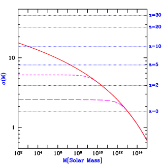
Figure 14: Mass fluctuations and collapse thresholds in cold dark matter models. The horizontal dotted lines show the value of the extrapolated collapse overdensity $\delta_{\rm crit}(z)$ at the indicated redshifts. Also shown is the value of $\sigma(M)$ for the cosmological parameters given in the text (solid curve), as well as $\sigma(M)$ for a power spectrum with a cutoff below a mass $M=1.7\times 10^{8}M_{\odot}$ (short-dashed curve), or $M=1.7\times 10^{11}M_{\odot}$ (long-dashed curve). The intersection of the horizontal lines with the other curves indicate, at each redshift $z$, the mass scale (for each model) at which a $1-\sigma$ fluctuation is just collapsing at $z$ (see the discussion in the text).

Also shown in Figure 14 is the effect of cutting off the power spectrum on small scales. The short-dashed curve corresponds to the case where the power spectrum is set to zero above a comoving wavenumber $k=10\,{\rm Mpc}^{-1}$, which corresponds to a mass $M=1.7\times 10^{8}M_{\odot}$. The long-dashed curve corresponds to a more radical cutoff above $k=1\,{\rm Mpc}^{-1}$, or below $M=1.7\times 10^{11}M_{\odot}$. A cutoff severely reduces the abundance of low-mass halos, and the finite value of $\sigma(M=0)$ implies that at all redshifts some fraction of the dark matter does not fall into halos. At high redshifts where $\delta_{\rm crit}(z)\gg\sigma(M=0)$, all halos are rare and only a small fraction of the dark matter lies in halos. In particular, this can affect the abundance of halos at the time of reionization, and thus the observed limits on reionization constrain scenarios which include a small-scale cutoff in the power spectrum BHO00 .

In figures 15 – 18 we show explicitly the properties of collapsing halos which represent $1-\sigma$, $2-\sigma$, and $3-\sigma$ fluctuations (corresponding in all cases to the curves in order from bottom to top), as a function of redshift. No cutoff is applied to the power spectrum. Figure 15 shows the halo mass, Figure 16 the virial radius, Figure 17 the virial temperature (with $\mu$ in equation (92) set equal to $0.6$, although low temperature halos contain neutral gas) as well as circular velocity, and Figure 18 shows the total binding energy of these halos. In figures 15 and 17, the dotted curves indicate the minimum virial temperature required for efficient cooling with primordial atomic species only (upper curve) or with the addition of molecular hydrogen (lower curve). Figure 18 shows the binding energy of dark matter halos. The binding energy of the baryons is a factor $\sim\Omega_{b}/\Omega_{m}\sim 15\%$ smaller, if they follow the dark matter. Except for this constant factor, the figure shows the minimum amount of energy that needs to be deposited into the gas in order to unbind it from the potential well of the dark matter. For example, the hydrodynamic energy released by a single supernovae, $\sim 10^{51}~{}{\rm erg}$, is sufficient to unbind the gas in all $1-\sigma$ halos at $z>5$ and in all $2-\sigma$ halos at $z>12$.

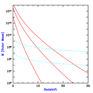
Figure 15: Characteristic properties of collapsing halos: Halo mass. The solid curves show the mass of collapsing halos which correspond to $1-\sigma$, $2-\sigma$, and $3-\sigma$ fluctuations (in order from bottom to top). The dotted curves show the mass corresponding to the minimum temperature required for efficient cooling with primordial atomic species only (upper curve) or with the addition of molecular hydrogen (lower curve).

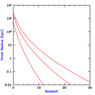
Figure 16: Characteristic properties of collapsing halos: Halo virial radius. The curves show the virial radius of collapsing halos which correspond to $1-\sigma$, $2-\sigma$, and $3-\sigma$ fluctuations (in order from bottom to top).

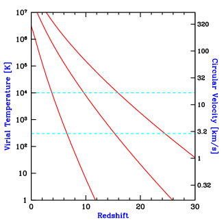
Figure 17: Characteristic properties of collapsing halos: Halo virial temperature and circular velocity. The solid curves show the virial temperature (or, equivalently, the circular velocity) of collapsing halos which correspond to $1-\sigma$, $2-\sigma$, and $3-\sigma$ fluctuations (in order from bottom to top). The dotted curves show the minimum temperature required for efficient cooling with primordial atomic species only (upper curve) or with the addition of molecular hydrogen (lower curve).

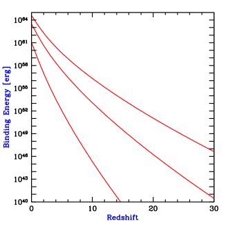
Figure 18: Characteristic properties of collapsing halos: Halo binding energy. The curves show the total binding energy of collapsing halos which correspond to $1-\sigma$, $2-\sigma$, and $3-\sigma$ fluctuations (in order from bottom to top).

At $z=5$, the halo masses which correspond to $1-\sigma$, $2-\sigma$, and $3-\sigma$ fluctuations are $1.8\times 10^{7}M_{\odot}$, $3.0\times 10^{10}M_{\odot}$, and $7.0\times 10^{11}M_{\odot}$, respectively. The corresponding virial temperatures are $2.0\times 10^{3}$ K, $2.8\times 10^{5}$ K, and $2.3\times 10^{6}$ K. The equivalent circular velocities are 7.5 ${\rm km\ s}^{-1}$, 88 ${\rm km\ s}^{-1}$, and 250 ${\rm km\ s}^{-1}$. At $z=10$, the $1-\sigma$, $2-\sigma$, and $3-\sigma$ fluctuations correspond to halo masses of $1.3\times 10^{3}M_{\odot}$, $5.7\times 10^{7}M_{\odot}$, and $4.8\times 10^{9}M_{\odot}$, respectively. The corresponding virial temperatures are 6.2 K, $7.9\times 10^{3}$ K, and $1.5\times 10^{5}$ K. The equivalent circular velocities are 0.41 ${\rm km\ s}^{-1}$, 15 ${\rm km\ s}^{-1}$, and 65 ${\rm km\ s}^{-1}$. Atomic cooling is efficient at $T_{\rm vir}>10^{4}$ K, or a circular velocity $V_{c}>17\ {\rm km\ s}^{-1}$. This corresponds to a $1.2-\sigma$ fluctuation and a halo mass of $2.1\times 10^{8}M_{\odot}$ at $z=5$, and a $2.1-\sigma$ fluctuation and a halo mass of $8.3\times 10^{7}M_{\odot}$ at $z=10$. Molecular hydrogen provides efficient cooling down to $T_{\rm vir}\sim 300$ K, or a circular velocity $V_{c}\sim 2.9\ {\rm km\ s}^{-1}$. This corresponds to a $0.81-\sigma$ fluctuation and a halo mass of $1.1\times 10^{6}M_{\odot}$ at $z=5$, and a $1.4-\sigma$ fluctuation and a halo mass of $4.3\times 10^{5}M_{\odot}$ at $z=10$.

In Figure 19 we show the halo mass function $dn/d\ln(M)$ at several different redshifts: $z=0$ (solid curve), $z=5$ (dotted curve), $z=10$ (short-dashed curve), $z=20$ (long-dashed curve), and $z=30$ (dot-dashed curve). Note that the mass function does not decrease monotonically with redshift at all masses. At the lowest masses, the abundance of halos is higher at $z>0$ than at $z=0$.

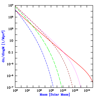
Figure 19: Halo mass function at several redshifts: $z=0$ (solid curve), $z=5$ (dotted curve), $z=10$ (short-dashed curve), $z=20$ (long-dashed curve), and $z=30$ (dot-dashed curve).

4.2 The Excursion-Set (Extended Press-Schechter) Formalism

The usual Press-Schechter formalism makes no attempt to deal with the correlations between halos or between different mass scales. In particular, this means that while it can generate a distribution of halos at two different epochs, it says nothing about how particular halos in one epoch are related to those in the second. We therefore would like some method to predict, at least statistically, the growth of individual halos via accretion and mergers. Even restricting ourselves to spherical collapse, such a model must utilize the full spherically-averaged density profile around a particular point. The potential correlations between the mean overdensities at different radii make the statistical description substantially more difficult.

The excursion set formalism (Bond et al. 1991 bond91 ) seeks to describe the statistics of halos by considering the statistical properties of $\overline{\delta}(R)$, the average overdensity within some spherical window of characteristic radius $R$, as a function of $R$. While the Press-Schechter model depends only on the Gaussian distribution of $\overline{\delta}$ for one particular $R$, the excursion set considers all $R$. Again the connection between a value of the linear regime $\delta$ and the final state is made via the spherical collapse solution, so that there is a critical value $\delta_{c}(z)$ of $\overline{\delta}$ which is required for collapse at a redshift $z$.

For most choices of window function, the functions $\overline{\delta}(R)$ are correlated from one $R$ to another such that it is prohibitively difficult to calculate the desired statistics directly [although Monte Carlo realizations are possible bond91 ]. However, for one particular choice of a window function, the correlations between different $R$ greatly simplify and many interesting quantities may be calculated bond91 ; LC93 . The key is to use a $k$-space top-hat window function, namely $W_{k}=1$ for all $k$ less than some critical $k_{c}$ and $W_{k}=0$ for $k>k_{c}$. This filter has a spatial form of $W(r)\>\propto\>j_{1}(k_{c}r)/k_{c}r$, which implies a volume $6\pi^{2}/k^{3}_{c}$ or mass $6\pi^{2}\rho_{b}/k^{3}_{c}$. The characteristic radius of the filter is $\sim k^{-1}_{c}$, as expected. Note that in real space, this window function converges very slowly, due only to a sinusoidal oscillation, so the region under study is rather poorly localized.

The great advantage of the sharp $k$-space filter is that the difference at a given point between $\overline{\delta}$ on one mass scale and that on another mass scale is statistically independent from the value on the larger mass scale. With a Gaussian random field, each $\delta_{k}$ is Gaussian distributed independently from the others. For this filter,

$$\overline{\delta}(M)=\int_{k<k_{c}(M)}\frac{d^{3}k}{(2\pi)^{3}}\delta_{k},$$ (99)

meaning that the overdensity on a particular scale is simply the sum of the random variables $\delta_{k}$ interior to the chosen $k_{c}$. Consequently, the difference between the $\overline{\delta}(M)$ on two mass scales is just the sum of the $\delta_{k}$ in the spherical shell between the two $k_{c}$, which is independent from the sum of the $\delta_{k}$ interior to the smaller $k_{c}$. Meanwhile, the distribution of $\overline{\delta}(M)$ given no prior information is still a Gaussian of mean zero and variance

$$\sigma^{2}(M)=\frac{1}{2\pi^{2}}\int_{k<k_{c}(M)}dk\>k^{2}P(k).$$ (100)

If we now consider $\overline{\delta}$ as a function of scale $k_{c}$, we see that we begin from $\overline{\delta}=0$ at $k_{c}=0\>(M=\infty)$ and then add independently random pieces as $k_{c}$ increases. This generates a random walk, albeit one whose stepsize varies with $k_{c}$. We then assume that, at redshift $z$, a given function $\overline{\delta}(k_{c})$ represents a collapsed mass $M$ corresponding to the $k_{c}$ where the function first crosses the critical value $\delta_{c}(z)$. With this assumption, we may use the properties of random walks to calculate the evolution of the mass as a function of redshift.

It is now easy to rederive the Press-Schechter mass function, including the previously unexplained factor of 2 bond91 ; LC93 ; Whi94 . The fraction of mass elements included in halos of mass less than $M$ is just the probability that a random walk remains below $\delta_{c}(z)$ for all $k_{c}$ less than $K_{c}$, the filter cutoff appropriate to $M$. This probability must be the complement of the sum of the probabilities that: (a) $\overline{\delta}(K_{c})>\delta_{c}(z)$; or that (b) $\overline{\delta}(K_{c})<\delta_{c}(z)$ but $\overline{\delta}(k^{\prime}_{c})>\delta_{c}(z)$ for some $k^{\prime}_{c}<K_{c}$. But these two cases in fact have equal probability; any random walk belonging to class (a) may be reflected around its first upcrossing of $\delta_{c}(z)$ to produce a walk of class (b), and vice versa. Since the distribution of $\overline{\delta}(K_{c})$ is simply Gaussian with variance $\sigma^{2}(M)$, the fraction of random walks falling into class (a) is simply $(1/\sqrt{2\pi\sigma^{2}})\int_{\delta_{c}(z)}^{\infty}d\delta\;\exp\{-\delta^{2}/2\sigma^{2}(M)\}$. Hence, the fraction of mass elements included in halos of mass less than $M$ at redshift $z$ is simply

$$F(<M)=1-2\times\frac{1}{\sqrt{2\pi\sigma^{2}}}\int_{\delta_{c}(z)}^{\infty}d\delta\>\exp\{-\delta^{2}/2\sigma^{2}(M)\}$$ (101)

which may be differentiated to yield the Press-Schechter mass function. We may now go further and consider how halos at one redshift are related to those at another redshift. If we are given that a halo of mass $M_{2}$ exists at redshift $z_{2}$, then we know that the random function $\overline{\delta}(k_{c})$ for each mass element within the halo first crosses $\delta(z_{2})$ at $k_{c2}$ corresponding to $M_{2}$. Given this constraint, we may study the distribution of $k_{c}$ where the function $\overline{\delta}(k_{c})$ crosses other thresholds. It is particularly easy to construct the probability distribution for when trajectories first cross some $\delta_{c}(z_{1})\>>\>\delta_{c}(z_{2})$ (implying $z_{1}\>>\>z_{2}$); clearly this occurs at some $k_{c1}\>>k_{c2}$. This problem reduces to the previous one if we translate the origin of the random walks from $(k_{c},\overline{\delta})=(0,0)\>{\rm to}\>(k_{c2},\delta_{c}(z_{2}))$. We therefore find the distribution of halo masses $M_{1}$ that a mass element finds itself in at redshift $z_{1}$ given that it is part of a larger halo of mass $M_{2}$ at a later redshift $z_{2}$ is bond91 ; Bow91 )

$$\begin{split}&\frac{dP}{dM_{1}}(M_{1},z_{1}|M_{2},z_{2})=\\ &\sqrt{\frac{2}{\pi}}\frac{\delta_{c}(z_{1})-\delta_{c}(z_{2})}{[\sigma^{2}(M_{1})-\sigma^{2}(M_{2})]^{3/2}}\left|\frac{d\sigma(M_{1})}{dM_{1}}\right|\exp\left\{-\frac{[\delta_{c}(z_{1})-\delta_{c}(z_{2})]^{2}}{2[\sigma^{2}(M_{1})-\sigma^{2}(M_{2})]}\right\}.\end{split}$$ (102)

This may be rewritten as saying that the quantity

$$\tilde{v}=\frac{\delta_{c}(z_{1})-\delta_{c}(z_{2})}{\sqrt{\sigma^{2}(M_{1})-\sigma^{2}(M_{2})}}$$ (103)

is distributed as the positive half of a Gaussian with unit variance; equation (103) may be inverted to find $M_{1}(\tilde{v})$.

We seek to interpret the statistics of these random walks as those of merging and accreting halos. For a single halo, we may imagine that as we look back in time, the object breaks into ever smaller pieces, similar to the branching of a tree. Equation (102) is the distribution of the sizes of these branches at some given earlier time. However, using this description of the ensemble distribution to generate Monte Carlo realizations of single merger trees has proven to be difficult. In all cases, one recursively steps back in time, at each step breaking the final object into two or more pieces. An elaborate scheme (Kauffmann & White 1993 KW93 ) picks a large number of progenitors from the ensemble distribution and then randomly groups them into sets with the correct total mass. This generates many (hundreds) possible branching schemes of equal likelihood. A simpler scheme (Lacey & Cole 1993 LC93 ) assumes that at each time step, the object breaks into two pieces. One value from the distribution (102) then determines the mass ratio of the two branchs.

One may also use the distribution of the ensemble to derive some additional analytic results. A useful example is the distribution of the epoch at which an object that has mass $M_{2}$ at redshift $z_{2}$ has accumulated half of its mass LC93 . The probability that the formation time is earlier than $z_{1}$ is equal to the probability that at redshift $z_{1}$ a progenitor whose mass exceeds $M_{2}/2$ exists:

$$P(z_{f}>z_{1})=\int_{M_{2}/2}^{M_{2}}\frac{M_{2}}{M}\frac{dP}{dM}(M,z_{1}|M_{2},z_{2})dM,$$ (104)

where $dP/dM$ is given in equation (102). The factor of $M_{2}/M$ corrects the counting from mass weighted to number weighted; each halo of mass $M_{2}$ can have only one progenitor of mass greater than $M_{2}/2$. Differentiating equation (104) with respect to time gives the distribution of formation times. This analytic form is an excellent match to scale-free N-body simulations LC94 . On the other hand, simple Monte Carlo implementations of equation (102) produce formation redshifts about 40% higher LC93 . As there may be correlations between the various branches, there is no unique Monte Carlo scheme.

Numerical tests of the excursion set formalism are quite encouraging. Its predictions for merger rates are in very good agreement with those measured in scale-free N-body simulations for mass scales down to around 10% of the nonlinear mass scale (that scale at which $\sigma_{M}=1$ ), and distributions of formation times closely match the analytic predictions LC94 . The model appears to be a promising method for tracking the merging of halos, with many applications to cluster and galaxy formation modeling. In particular, one may use the formalism as the foundation of semi-analytic galaxy formation models KWG93 . The excursion set formalism may also be used to derive the correlations of halos in the nonlinear regime mw96 .

4.3 Response of Baryons to Nonlinear Dark Matter Potentials

The dark matter is assumed to be cold and to dominate gravity, and so its collapse and virialization proceeds unimpeded by pressure effects. In order to estimate the minimum mass of baryonic objects, we must go beyond linear perturbation theory and examine the baryonic mass that can accrete into the final gravitational potential well of the dark matter.

For this purpose, we assume that the dark matter had already virialized and produced a gravitational potential $\phi({\bf r})$ at a redshift $z_{\rm vir}$ (with $\phi\rightarrow 0$ at large distances, and $\phi<0$ inside the object) and calculate the resulting overdensity in the gas distribution, ignoring cooling (an assumption justified by spherical collapse simulations which indicate that cooling becomes important only after virialization; see Haiman et al. 1996 Haiman ).

After the gas settles into the dark matter potential well, it satisfies the hydrostatic equilibrium equation,

$$\nabla p_{\rm b}=-\rho_{\rm b}\nabla\phi$$ (105)

where $p_{\rm b}$ and $\rho_{\rm b}$ are the pressure and mass density of the gas. At $z<100$ the gas temperature is decoupled from the CMB, and its pressure evolves adiabatically (ignoring atomic or molecular cooling),

$${p_{\rm b}\over{\bar{p}}_{\rm b}}=\left({\rho_{\rm b}\over{\bar{\rho}}_{\rm b}}\right)^{5/3}$$ (106)

where a bar denotes the background conditions. We substitute equation (106) into (105) and get the solution,

$${\rho_{\rm b}\over{\bar{\rho}}_{\rm b}}=\left(1-{2\over 5}{\mu m_{p}\phi\over{k\bar{T}}}\right)^{3/2}$$ (107)

where ${\bar{T}}={\bar{p}}_{\rm b}\mu m_{p}/(k{\bar{\rho}}_{\rm b})$ is the background gas temperature. If we define $T_{\rm vir}=-{1\over 3}m_{p}\phi/k$ as the virial temperature for a potential depth $-\phi$, then the overdensity of the baryons at the virialization redshift is

$$\delta_{\rm b}={\rho_{\rm b}\over{\bar{\rho}}_{\rm b}}-1=\left(1+{6\over 5}{T_{\rm vir}\over{\bar{T}}}\right)^{3/2}-1.$$ (108)

This solution is approximate for two reasons: (i) we assumed that the gas is stationary throughout the entire region and ignored the transitions to infall and the Hubble expansion at the interface between the collapsed object and the background intergalactic medium (henceforth IGM), and (ii) we ignored entropy production at the virialization shock surrounding the object. Nevertheless, the result should provide a better estimate for the minimum mass of collapsed baryonic objects than the Jeans mass does, since it incorporates the nonlinear potential of the dark matter.

We may define the threshold for the collapse of baryons by the criterion that their mean overdensity, $\delta_{\rm b}$, exceeds a value of 100, amounting to $>50\%$ of the baryons that would assemble in the absence of gas pressure, according to the spherical top-hat collapse model. Equation (108) then implies that $T_{\rm vir}>17.2\,{\bar{T}}$.

As mentioned before, the gas temperature evolves at $z<160$ according to the relation ${\bar{T}}\approx 170[(1+z)/100]^{2}\ {\rm K}$. This implies that baryons are overdense by $\delta_{\rm b}>100$ only inside halos with a virial temperature $T_{\rm vir}>2.9\times 10^{3}~{}[(1+z)/100]^{2}\ {\rm K}$. Based on the top-hat model, this implies a minimum halo mass for baryonic objects of

$$M_{\rm min}=5.0\times 10^{3}\left({\Omega_{m}h^{2}\over 0.15}\right)^{-1/2}\left({\Omega_{b}h^{2}\over 0.022}\right)^{-3/5}\left({1+z\over 10}\right)^{3/2}~{}M_{\odot},$$ (109)

where we consider sufficiently high redshifts so that ${\Omega_{m}^{\,z}}\approx 1$. This minimum mass is coincidentally almost identical to the naive Jeans mass calculation of linear theory in equation (62) despite the fact that it incorporates shell crossing by the dark matter, which is not accounted for by linear theory. Unlike the Jeans mass, the minimum mass depends on the choice for an overdensity threshold [taken arbitrarily as $\delta_{\rm b}>100$ in equation (109)]. To estimate the minimum halo mass which produces any significant accretion we set, e.g., $\delta_{\rm b}=5$, and get a mass which is lower than $M_{\rm min}$ by a factor of 27.

Of course, once the first stars and quasars form they heat the surrounding IGM by either outflows or radiation. As a result, the Jeans mass which is relevant for the formation of new objects changes G097 ; g00 ). The most dramatic change occurs when the IGM is photo-ionized and is consequently heated to a temperature of $\sim(1$–$2)\times 10^{4}$ K.

5 Fragmentation of the First Gaseous Objects to Stars

5.1 Star Formation

As mentioned in the preface, the fragmentation of the first gaseous objects is a well-posed physics problem with well specified initial conditions, for a given power-spectrum of primordial density fluctuations. This problem is ideally suited for three-dimensional computer simulations, since it cannot be reliably addressed in idealized 1D or 2D geometries.

Recently, two groups have attempted detailed 3D simulations of the formation process of the first stars in a halo of $\sim 10^{6}M_{\odot}$ by following the dynamics of both the dark matter and the gas components, including H₂ chemistry and cooling. Bromm, Coppi, & Larson (1999) BCL99 have used a Smooth Particle Hydrodynamics (SPH) code to simulate the collapse of a top-hat overdensity with a prescribed solid-body rotation (corresponding to a spin parameter $\lambda=5\%$) and additional small perturbations with $P(k)\propto k^{-3}$ added to the top-hat profile. Abel et al. (2002) ABN02 isolated a high-density filament out of a larger simulated cosmological volume and followed the evolution of its density maximum with exceedingly high resolution using an Adaptive Mesh Refinement (AMR) algorithm.

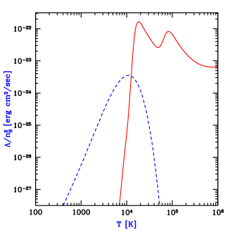
Figure 20: Cooling rates as a function of temperature for a primordial gas composed of atomic hydrogen and helium, as well as molecular hydrogen, in the absence of any external radiation. We assume a hydrogen number density $n_{H}=0.045\ {\rm cm}^{-3}$, corresponding to the mean density of virialized halos at $z=10$. The plotted quantity $\Lambda/n_{H}^{2}$ is roughly independent of density (unless $n_{H}>10\ {\rm cm}^{-3}$), where $\Lambda$ is the volume cooling rate (in erg/sec/cm³). The solid line shows the cooling curve for an atomic gas, with the characteristic peaks due to collisional excitation of H1 and He2. The dashed line shows the additional contribution of molecular cooling, assuming a molecular abundance equal to $1\%$ of $n_{H}$.

The generic results of Bromm et al. (1999 BCL99 ; see also Bromm 2000 Bro00 ) are illustrated in Figure 21. The collapsing region forms a disk which fragments into many clumps. The clumps have a typical mass $\sim 10^{2}$–$10^{3}M_{\odot}$. This mass scale corresponds to the Jeans mass for a temperature of $\sim 500$K and the density $\sim 10^{4}~{}{\rm cm^{-3}}$ where the gas lingers because its cooling time is longer than its collapse time at that point (see Fig. 22). Each clump accretes mass slowly until it exceeds the Jeans mass and collapses at a roughly constant temperature (isothermally) due to H₂ cooling that brings the gas to a fixed temperature floor. The clump formation efficiency is high in this simulation due to the synchronized collapse of the overall top-hat perturbation.

Figure 21: Numerical results from Bromm et al. (1999) BCL99 , showing gas properties at $z=31.2$ for a collapsing slightly inhomogeneous top-hat region with a prescribed solid-body rotation. (a) Free electron fraction (by number) vs. hydrogen number density (in cm^-3). At densities exceeding $n\sim 10^{3}$ cm^-3, recombination is very efficient, and the gas becomes almost completely neutral. (b) Molecular hydrogen fraction vs. number density. After a quick initial rise, the H₂ fraction approaches the asymptotic value of $f\sim 10^{-3}$, due to the H^- channel. (c) Gas temperature vs. number density. At densities below $\sim 1$ cm^-3, the gas temperature rises because of adiabatic compression until it reaches the virial value of $T_{vir}\simeq 5000$ K. At higher densities, cooling due to H₂ drives the temperature down again, until the gas settles into a quasi-hydrostatic state at $T\sim 500$ K and $n\sim 10^{4}$ cm^-3. Upon further compression due to accretion and the onset of gravitational collapse, the gas shows a further modest rise in temperature. (d) Jeans mass (in $M_{\odot}$) vs. number density. The Jeans mass reaches a value of $M_{J}\sim 10^{3}M_{\odot}$ for the quasi-hydrostatic gas in the center of the potential well, and reaches the resolution limit of the simulation, $M_{\rm res}\simeq 200M_{\odot}$, for densities close to $n=10^{8}$ cm^-3.

Figure 22: Gas and clump morphology at $z=28.9$ in the simulation of Bromm et al. (1999) BCL99 . Top row: The remaining gas in the diffuse phase. Bottom row: Distribution of clumps. The numbers next to the dots denote clump mass in units of $M_{\odot}$. Left panels: Face-on view. Right panels: Edge-on view. The length of the box is 30 pc. The gas has settled into a flattened configuration with two dominant clumps of mass close to $20,000M_{\odot}$. During the subsequent evolution, the clumps survive without merging, and grow in mass only slightly by accretion of surrounding gas.

Bromm (2000) Bro00 has simulated the collapse of one of the above-mentioned clumps with $\sim 1000M_{\odot}$ and demonstrated that it does not tend to fragment into sub-components. Rather, the clump core of $\sim 100M_{\odot}$ free-falls towards the center leaving an extended envelope behind with a roughly isothermal density profile. At very high gas densities, three-body reactions become important in the chemistry of H₂. Omukai & Nishi (1998) ON1998 have included these reactions as well as radiative transfer and followed the collapse in spherical symmetry up to stellar densities. Radiation pressure from nuclear burning at the center is unlikely to reverse the infall as the stellar mass builds up. These calculations indicate that each clump may end as a single massive star; however, it is conceivable that angular momentum may eventually halt the collapsing cloud and lead to the formation of a binary stellar system instead.

The Jeans mass, which is defined based on small fluctuations in a background of uniform density, does not strictly apply in the context of collapsing gas cores. We can instead use a slightly modified critical mass known as the Bonnor-Ebert mass Bo56 ; Eb55 . For baryons in a background of uniform density $\rho_{b}$, perturbations are unstable to gravitational collapse in a region more massive than the Jeans mass. Instead of a uniform background, we consider a spherical, non-singular, isothermal, self-gravitating gas in hydrostatic equilibrium, i.e., a centrally-concentrated object which more closely resembles the gas cores found in the above-mentioned simulations. In this case, small fluctuations are unstable and lead to collapse if the sphere is more massive than the Bonnor-Ebert mass $M_{\rm BE}$, given by the same expression the Jeans Mass but with a different coefficient (1.2 instead of 2.9) and with $\rho_{b}$ denoting in this case the gas (volume) density at the surface of the sphere,

$$M_{\rm BE}=1.2\,\frac{1}{\sqrt{\rho_{b}}}\,\left(\frac{kT}{G\mu m_{p}}\right)^{3/2}\ .$$ (110)

In their simulation, Abel et al. (2000)Abel adopted the actual cosmological density perturbations as initial conditions. The simulation focused on the density peak of a filament within the IGM, and evolved it to very high densities (Fig. 23). Following the initial collapse of the filament, a clump core formed with $\sim 200M_{\odot}$, amounting to only $\sim 1\%$ of the virialized mass. Subsequently due to slow cooling, the clump collapsed subsonically in a state close to hydrostatic equilibrium (see Fig. 24). Unlike the idealized top-hat simulation of Bromm et al. (2001) BKL2001 , the collapse of the different clumps within the filament is not synchronized. Once the first star forms at the center of the first collapsing clump, it is likely to affect the formation of other stars in its vicinity.

As soon as nuclear burning sets in the core of the proto-star, the radiation emitted by the star starts to affect the infall of the surrounding gas towards it. The radiative feedback involves photo-dissociation of H₂, Ly$\alpha$ radiation pressure, and photo-evaporation of the accretion disk. Tan & McKee Tan2003 studied these effects by extrapolating analytically the infall of gas from the final snapshot of the above resolution-limited simulations to the scale of a proto-star; they concluded that nuclear burning (and hence the feedback) starts when the proton-star accretes $\sim 30M_{\odot}$ and accretion is likely to be terminated when the star reaches $\sim 200M_{\odot}$.

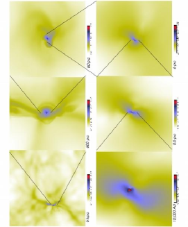
Figure 23: Zooming in on the core of a star forming region with the Adaptive Mesh Refinement simulation of Abel et al. (2000) Abel . The panels show different length scales, decreasing clockwise by an order of magnitude between adjacent panels. Note the large dynamic range of scales which are being resolved, from 6 kpc (top left panel) down to 10,000 AU (bottom left panel).

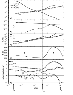
Figure 24: Gas profiles from the simulation of Abel et al. (2000)Abel . The cell size on the finest grid corresponds to $0.024$ pc, while the simulation box size corresponds to 6.4 kpc. Shown are spherically-averaged mass-weighted profiles around the baryon density peak shortly before a well defined fragment forms ($z=19.1$). Panel (a) shows the baryonic number density, enclosed gas mass in solar mass, and the local Bonnor-Ebert mass $M_{\rm BE}$ (see text). Panel (b) plots the molecular hydrogen fraction (by number) $f_{H_{2}}$ and the free electron fraction $x$. The H₂ cooling time, $t_{H_{2}}$, the time it takes a sound wave to travel to the center, $t_{\rm cross}$, and the free–fall time $t_{\rm ff}=[3\pi/(32G\rho)]^{1/2}$ are given in panel (c). Panel (d) gives the temperature in K as a function of radius. The bottom panel gives the local sound speed, $c_{s}$ (solid line with circles), the rms radial velocities of the dark matter (dashed line) and the gas (dashed line with asterisks) as well as the rms gas velocity (solid line with square symbols). The vertical dotted line indicates the radius ($\sim 5$ pc) at which the gas has reached its minimum temperature allowed by H₂ cooling. The virial radius of the $5.6\times 10^{6}M_{\odot}$ halo is 106 pc.

If the clumps in the above simulations end up forming individual very massive stars, then these stars will likely radiate copious amounts of ionizing radiation CBA84 ; TS00 ; BKL2001 and expel strong winds. Hence, the stars will have a large effect on their interstellar environment, and feedback is likely to control the overall star formation efficiency. This efficiency is likely to be small in galactic potential wells which have a virial temperature lower than the temperature of photoionized gas, $\sim 10^{4}$K. In such potential wells, the gas may go through only a single generation of star formation, leading to a “suicidal” population of massive stars.

The final state in the evolution of these stars is uncertain; but if their mass loss is not too extensive, then they are likely to end up as black holes CBA84 ; FWH00 . The remnants may provide the seeds of quasar black holes Lar99 . Some of the massive stars may end their lives by producing gamma-ray bursts. If so then the broad-band afterglows of these bursts could provide a powerful tool for probing the epoch of reionization LR00 ; CL00 ). There is no better way to end the dark ages than with $\gamma$-ray burst fireworks.

Where are the first stars or their remnants located today? The very first stars formed in rare high-$\sigma$ peaks and hence are likely to populate the cores of present-day galaxies WS99 . However, the bulk of the stars which formed in low-mass systems at later times are expected to behave similarly to the collisionless dark matter particles and populate galaxy halos Loe98 .

5.2 The Mass Function of Stars

Currently, we do not have direct observational constraints on how the first stars, the so-called Population III stars, formed at the end of the cosmic dark ages. It is, therefore, instructive to briefly summarize what we have learned about star formation in the present-day Universe, where theoretical reasoning is guided by a wealth of observational data (see Pud2002 for a recent review).

Population I stars form out of cold, dense molecular gas that is structured in a complex, highly inhomogeneous way. The molecular clouds are supported against gravity by turbulent velocity fields and pervaded on large scales by magnetic fields. Stars tend to form in clusters, ranging from a few hundred up to $\sim 10^{6}$ stars. It appears likely that the clustered nature of star formation leads to complicated dynamics and tidal interactions that transport angular momentum, thus allowing the collapsing gas to overcome the classical centrifugal barrier Lar2002 . The initial mass function (IMF) of Pop I stars is observed to have the approximate Salpeter form (e.g., Kr02 )

$$\frac{{\rm d}N}{{\rm dlog}M}\propto M^{x}\mbox{\ ,}$$ (111)

where

$$x\simeq\left\{\begin{array}[]{rl}-1.35&\mbox{for \ }M\geq 0.5M_{\odot}\\ 0.0&\mbox{for \ }0.007\leq M\leq 0.5M_{\odot}\\ \end{array}\right.\mbox{\ .}$$ (112)

The lower cutoff in mass corresponds roughly to the opacity limit for fragmentation. This limit reflects the minimum fragment mass, set when the rate at which gravitational energy is released during the collapse exceeds the rate at which the gas can cool (e.g., MJR1976 ). The most important feature of the observed IMF is that $\sim 1M_{\odot}$ is the characteristic mass scale of Pop I star formation, in the sense that most of the mass goes into stars with masses close to this value. In Figure 25, we show the result from a recent hydrodynamical simulation of the collapse and fragmentation of a molecular cloud core BBB2002 ; BBB2003 . This simulation illustrates the highly dynamic and chaotic nature of the star formation process.

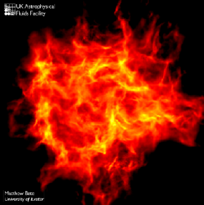
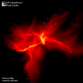
Figure 25: A hydrodynamic simulation of the collapse and fragmentation of a turbulent molecular cloud in the present-day Universe (from BBB2003 ). The cloud has a mass of $50M_{\odot}$. The panels show the column density through the cloud, and span a scale of 0.4 pc across. Left: The initial phase of the collapse. The turbulence organizes the gas into a network of filaments, and decays thereafter through shocks. Right: A snapshot taken near the end of the simulation, after 1.4 initial free-fall times of $2\times 10^{5}$yr. Fragmentation has resulted in $\sim 50$ stars and brown dwarfs. The star formation efficiency is $\sim 10$% on the scale of the overall cloud, but can be much larger in the dense sub-condensations. This result is in good agreement with what is observed in local star-forming regions.

The metal-rich chemistry, magnetohydrodynamics, and radiative transfer involved in present-day star formation is complex, and we still lack a comprehensive theoretical framework that predicts the IMF from first principles. Star formation in the high redshift Universe, on the other hand, poses a theoretically more tractable problem due to a number of simplifying features, such as: (i) the initial absence of heavy metals and therefore of dust; and (ii) the absence of dynamically-significant magnetic fields, in the pristine gas left over from the big bang. The cooling of the primordial gas does then only depend on hydrogen in its atomic and molecular form. Whereas in the present-day interstellar medium, the initial state of the star forming cloud is poorly constrained, the corresponding initial conditions for primordial star formation are simple, given by the popular $\Lambda$CDM model of cosmological structure formation. We now turn to a discussion of this theoretically attractive and important problem.

How did the first stars form? A complete answer to this question would entail a theoretical prediction for the Population III IMF, which is rather challenging. Let us start by addressing the simpler problem of estimating the characteristic mass scale of the first stars. As mentioned before, this mass scale is observed to be $\sim 1M_{\odot}$ in the present-day Universe.

Bromm & Loeb (2004) BL04 carried out idealized simulations of the protostellar accretion problem and estimated the final mass of a Population III star. Using the smoothed particle hydrodynamics (SPH) method, they included the chemistry and cooling physics relevant for the evolution of metal-free gas (see BCL02 for details). Improving on earlier work BCL99 ; BCL02 by initializing the simulations according to the $\Lambda$CDM model, they focused on an isolated overdense region that corresponds to a 3$\sigma-$peak BL04 : a halo containing a total mass of $10^{6}M_{\odot}$, and collapsing at a redshift $z_{\rm vir}\simeq 20$. In these runs, one high-density clump has formed at the center of the minihalo, possessing a gas mass of a few hundred solar masses. Soon after its formation, the clump becomes gravitationally unstable and undergoes runaway collapse. Once the gas clump has exceeded a threshold density of $10^{7}$ cm^-3, it is replaced by a sink particle which is a collisionless point-like particle that is inserted into the simulation. This choice for the density threshold ensures that the local Jeans mass is resolved throughout the simulation. The clump (i.e., sink particle) has an initial mass of $M_{\rm Cl}\simeq 200M_{\odot}$, and grows subsequently by ongoing accretion of surrounding gas. High-density clumps with such masses result from the chemistry and cooling rate of molecular hydrogen, H₂, which imprint characteristic values of temperature, $T\sim 200$ K, and density, $n\sim 10^{4}$ cm^-3, into the metal-free gas BCL02 . Evaluating the Jeans mass for these characteristic values results in $M_{J}\sim\mbox{\ a few \ }\times 10^{2}M_{\odot}$, which is close to the initial clump masses found in the simulations.

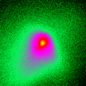
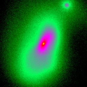
Figure 26: Collapse and fragmentation of a primordial cloud (from BL04 ). Shown is the projected gas density at a redshift $z\simeq 21.5$, briefly after gravitational runaway collapse has commenced in the center of the cloud. Left: The coarse-grained morphology in a box with linear physical size of 23.5 pc. At this time in the unrefined simulation, a high-density clump (sink particle) has formed with an initial mass of $\sim 10^{3}M_{\odot}$. Right: The refined morphology in a box with linear physical size of 0.5 pc. The central density peak, vigorously gaining mass by accretion, is accompanied by a secondary clump.

Figure 27: Accretion onto a primordial protostar (from BL04 ). The morphology of this accretion flow is shown in Fig. 26. Left: Accretion rate (in $M_{\odot}$ yr^-1) vs. time (in yr) since molecular core formation. Right: Mass of the central core (in $M_{\odot}$) vs. time. Solid line: Accretion history approximated as: $M_{\ast}\propto t^{0.45}$. Using this analytical approximation, we extrapolate that the protostellar mass has grown to $\sim 150M_{\odot}$ after $\sim 10^{5}$ yr, and to $\sim 700M_{\odot}$ after $\sim 3\times 10^{6}$ yr, the total lifetime of a very massive star.

The high-density clumps are clearly not stars yet. To probe the subsequent fate of a clump, Bromm & Loeb (2004) BL04 have re-simulated the evolution of the central clump with sufficient resolution to follow the collapse to higher densities. Figure 26 (right panel) shows the gas density on a scale of 0.5 pc, which is two orders of magnitude smaller than before. Several features are evident in this plot. First, the central clump does not undergo further sub-fragmentation, and is likely to form a single Population III star. Second, a companion clump is visible at a distance of $\sim 0.25$ pc. If negative feedback from the first-forming star is ignored, this companion clump would undergo runaway collapse on its own approximately $\sim 3$ Myr later. This timescale is comparable to the lifetime of a very massive star (VMS)BKL2001 . If the second clump was able to survive the intense radiative heating from its neighbor, it could become a star before the first one explodes as a supernova (SN). Whether more than one star can form in a low-mass halo thus crucially depends on the degree of synchronization of clump formation. Finally, the non-axisymmetric disturbance induced by the companion clump, as well as the angular momentum stored in the orbital motion of the binary system, allow the system to overcome the angular momentum barrier for the collapse of the central clump (see Lar2002 ).

The recent discovery of stars like HE0107-5240 with a mass of $0.8M_{\odot}$ and an iron abundance of ${\rm[Fe/H]}=-5.3$ Cr02 shows that at least some low mass stars could have formed out of extremely low-metallicity gas. The above simulations show that although the majority of clumps are very massive, a few of them, like the secondary clump in Fig. 26, are significantly less massive. Alternatively, low-mass fragments could form in the dense, shock-compressed shells that surround the first hypernovae MBH03 .

How massive were the first stars? Star formation typically proceeds from the ‘inside-out’, through the accretion of gas onto a central hydrostatic core. Whereas the initial mass of the hydrostatic core is very similar for primordial and present-day star formation ON1998 , the accretion process – ultimately responsible for setting the final stellar mass, is expected to be rather different. On dimensional grounds, the accretion rate is simply related to the sound speed cubed over Newton’s constant (or equivalently given by the ratio of the Jeans mass and the free-fall time): $\dot{M}_{\rm acc}\sim c_{s}^{3}/G\propto T^{3/2}$. A simple comparison of the temperatures in present-day star forming regions ($T\sim 10$ K) with those in primordial ones ($T\sim 200-300$ K) already indicates a difference in the accretion rate of more than two orders of magnitude.

The above refined simulation enables one to study the three-dimensional accretion flow around the protostar (see also OP2001 ; Rip2002 ; Tan2003 ). The gas may now reach densities of $10^{12}$ cm^-3 before being incorporated into a central sink particle. At these high densities, three-body reactions PSS1983 convert the gas into a fully molecular form. Figure 27 shows how the molecular core grows in mass over the first $\sim 10^{4}$ yr after its formation. The accretion rate (left panel) is initially very high, $\dot{M}_{\rm acc}\sim 0.1M_{\odot}$ yr^-1, and subsequently declines according to a power law, with a possible break at $\sim 5000$ yr. The mass of the molecular core (right panel), taken as an estimator of the proto-stellar mass, grows approximately as: $M_{\ast}\sim\int\dot{M}_{\rm acc}{\rm d}t\propto t^{0.45}$. A rough upper limit for the final mass of the star is then: $M_{\ast}(t=3\times 10^{6}{\rm yr})\sim 700M_{\odot}$. In deriving this upper bound, we have conservatively assumed that accretion cannot go on for longer than the total lifetime of a massive star.

Can a Population III star ever reach this asymptotic mass limit? The answer to this question is not yet known with any certainty, and it depends on whether the accretion from a dust-free envelope is eventually terminated by feedback from the star (e.g., OP2001 ; Rip2002 ; Tan2003 ; OI2002 ). The standard mechanism by which accretion may be terminated in metal-rich gas, namely radiation pressure on dust grains WC1987 , is evidently not effective for gas with a primordial composition. Recently, it has been speculated that accretion could instead be turned off through the formation of an H II region OI2002 , or through the photo-evaporation of the accretion disk Tan2003 . The termination of the accretion process defines the current unsolved frontier in studies of Population III star formation. Current simulations indicate that the first stars were predominantly very massive ($>30M_{\odot}$), and consequently rather different from present-day stellar populations. The crucial question then arises: How and when did the transition take place from the early formation of massive stars to that of low-mass stars at later times? We address this problem next.

The very first stars, marking the cosmic Renaissance of structure formation, formed under conditions that were much simpler than the highly complex environment in present-day molecular clouds. Subsequently, however, the situation rapidly became more complicated again due to the feedback from the first stars on the IGM. Supernova explosions dispersed the nucleosynthetic products from the first generation of stars into the surrounding gas (e.g., MFR01 ; MFM02 ; TSD02 ), including also dust grains produced in the explosion itself LH97 ; TodF01 . Atomic and molecular cooling became much more efficient after the addition of these metals. Moreover, the presence of ionizing cosmic rays, as well as of UV and X-ray background photons, modified the thermal and chemical behavior of the gas in important ways (e.g., MBA01 ; MBA03 ).

Early metal enrichment was likely the dominant effect that brought about the transition from Population III to Population II star formation. Recent numerical simulations of collapsing primordial objects with overall masses of $\sim 10^{6}M_{\odot}$, have shown that the gas has to be enriched with heavy elements to a minimum level of $Z_{\rm crit}\simeq 10^{-3.5}Z_{\odot}$, in order to have any effect on the dynamics and fragmentation properties of the system Om00 ; BFCL01 ; BrL03 . Normal, low-mass (Population II) stars are hypothesized to only form out of gas with metallicity $Z\geq Z_{\rm crit}$. Thus, the characteristic mass scale for star formation is expected to be a function of metallicity, with a discontinuity at $Z_{\rm crit}$ where the mass scale changes by $\sim$ two orders of magnitude. The redshift where this transition occurs has important implications for the early growth of cosmic structure, and the resulting observational signature (e.g., Wyithe03 ; FL03 ; MBH03 ; Sch02 ) include the extended nature of reionization FL05 .

For additional detailes about the properties of the first stars, see the comprehensive review by Bromm & Larson (2004) Bromm .

5.3 Gamma-ray Bursts: Probing the First Stars One Star at a Time

Gamma-Ray Bursts (GRBs) are believed to originate in compact remnants (neutron stars or black holes) of massive stars. Their high luminosities make them detectable out to the edge of the visible Universe CL00 ; LR00 . GRBs offer the opportunity to detect the most distant (and hence earliest) population of massive stars, the so-called Population III (or Pop III), one star at a time. In the hierarchical assembly process of halos which are dominated by cold dark matter (CDM), the first galaxies should have had lower masses (and lower stellar luminosities) than their low-redshift counterparts. Consequently, the characteristic luminosity of galaxies or quasars is expected to decline with increasing redshift. GRB afterglows, which already produce a peak flux comparable to that of quasars or starburst galaxies at $z\sim 1-2$, are therefore expected to outshine any competing source at the highest redshifts, when the first dwarf galaxies have formed in the Universe.

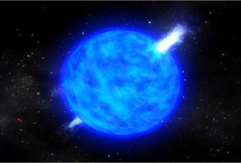
Figure 28: Illustration of a long-duration gamma-ray burst in the popular “collapsar” model. The collapse of the core of a massive star (which lost its hydrogen envelope) to a black hole generates two opposite jets moving out at a speed close to the speed of light. The jets drill a hole in the star and shine brightly towards an observer who happened to be located within with the collimation cones of the jets. The jets emenating from a single massive star are so bright that they can be seen across the Universe out to the epoch when the first stars have formed. Upcoming observations by the Swift satellite will have the sensitivity to reveal whether the first stars served as progenitors of gamma-ray bursts (for updates see http://swift.gsfc.nasa.gov/).

The first-year polarization data from the Wilkinson Microwave Anisotropy Probe (WMAP) indicates an optical depth to electron scattering of $\sim 17\pm 4$% after cosmological recombination Kog03 ; WMAP . This implies that the first stars must have formed at a redshift $z\sim$10–20, and reionized a substantial fraction of the intergalactic hydrogen around that time Cen03 ; CFW03 ; SL03 ; WL03 ; YBH04 . Early reionization can be achieved with plausible star formation parameters in the standard $\Lambda$CDM cosmology; in fact, the required optical depth can be achieved in a variety of very different ionization histories since WMAP places only an integral constraint on these histories HH03 . One would like to probe the full history of reionization in order to disentangle the properties and formation history of the stars that are responsible for it. GRB afterglows offer the opportunity to detect stars as well as to probe the metal enrichment level FL03 of the intervening IGM.

GRBs, the electromagnetically-brightest explosions in the Universe, should be detectable out to redshifts $z>10$ CL00 ; LR00 . High-redshift GRBs can be identified through infrared photometry, based on the Ly$\alpha$ break induced by absorption of their spectrum at wavelengths below $1.216\,\mu{\rm m}\,[(1+z)/10]$. Follow-up spectroscopy of high-redshift candidates can then be performed on a 10-meter-class telescope. Recently, the ongoing Swift mission Geh04 has detected a GRB originating at $z\simeq 6.3$ (e.g., Hai05 ), thus demonstrating the viability of GRBs as probes of the early Universe.

There are four main advantages of GRBs relative to traditional cosmic sources such as quasars:

(i) The GRB afterglow flux at a given observed time lag after the $\gamma$-ray trigger is not expected to fade significantly with increasing redshift, since higher redshifts translate to earlier times in the source frame, during which the afterglow is intrinsically brighter CL00 . For standard afterglow lightcurves and spectra, the increase in the luminosity distance with redshift is compensated by this cosmological time-stretching effect.

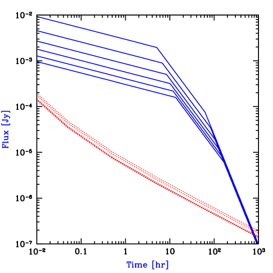
Figure 29: GRB afterglow flux as a function of time since the $\gamma$-ray trigger in the observer frame (taken from BL04 ). The flux (solid curves) is calculated at the redshifted Ly$\alpha$ wavelength. The dotted curves show the planned detection threshold for the James Webb Space Telescope (JWST), assuming a spectral resolution $R=5000$ with the near infrared spectrometer, a signal to noise ratio of 5 per spectral resolution element, and an exposure time equal to $20\%$ of the time since the GRB explosion (see http://www.ngst.stsci.edu/nms/main/ ). Each set of curves shows a sequence of redshifts, namely $z=5$, 7, 9, 11, 13, and 15, respectively, from top to bottom.

(ii) As already mentioned, in the standard $\Lambda$CDM cosmology, galaxies form hierarchically, starting from small masses and increasing their average mass with cosmic time. Hence, the characteristic mass of quasar black holes and the total stellar mass of a galaxy were smaller at higher redshifts, making these sources intrinsically fainter WL02 . However, GRBs are believed to originate from a stellar mass progenitor and so the intrinsic luminosity of their engine should not depend on the mass of their host galaxy. GRB afterglows are therefore expected to outshine their host galaxies by a factor that gets larger with increasing redshift.

(iii) Since the progenitors of GRBs are believed to be stellar, they likely originate in the most common star-forming galaxies at a given redshift rather than in the most massive host galaxies, as is the case for bright quasars GRBquasar . Low-mass host galaxies induce only a weak ionization effect on the surrounding IGM and do not greatly perturb the Hubble flow around them. Hence, the Ly$\alpha$ damping wing should be closer to the idealized unperturbed IGM case and its detailed spectral shape should be easier to interpret. Note also that unlike the case of a quasar, a GRB afterglow can itself ionize at most $\sim 4\times 10^{4}E_{51}M_{\odot}$ of hydrogen if its UV energy is $E_{51}$ in units of $10^{51}$ ergs (based on the available number of ionizing photons), and so it should have a negligible cosmic effect on the surrounding IGM.

(iv) GRB afterglows have smooth (broken power-law) continuum spectra unlike quasars which show strong spectral features (such as broad emission lines or the so-called “blue bump”) that complicate the extraction of IGM absorption features. In particular, the continuum extrapolation into the Ly$\alpha$ damping wing (the so-called Gunn-Peterson absorption trough) during the epoch of reionization is much more straightforward for the smooth UV spectra of GRB afterglows than for quasars with an underlying broad Ly$\alpha$ emission line GRBquasar .

The optical depth of the uniform IGM to Ly$\alpha$ absorption is given by (Gunn & Peterson 1965 GP ),

$$\tau_{s}={\pi e^{2}f_{\alpha}\lambda_{\alpha}n_{\rm H\,I~{}}(z_{s})\over m_{e}cH(z_{s})}\approx 6.45\times 10^{5}x_{\rm H\,I~{}}\left({\Omega_{b}h\over 0.03}\right)\left({\Omega_{m}\over 0.3}\right)^{-1/2}\left({1+z_{s}\over 10}\right)^{3/2}$$ (113)

where $H\approx 100h~{}{\rm km~{}s^{-1}~{}Mpc^{-1}}\Omega_{m}^{1/2}(1+z_{s})^{3/2}$ is the Hubble parameter at the source redshift $z_{s}>>1$, $f_{\alpha}=0.4162$ and $\lambda_{\alpha}=1216$Å  are the oscillator strength and the wavelength of the Ly$\alpha$ transition; $n_{\rm H\,I~{}}(z_{s})$ is the neutral hydrogen density at the source redshift (assuming primordial abundances); $\Omega_{m}$ and $\Omega_{b}$ are the present-day density parameters of all matter and of baryons, respectively; and $x_{\rm H\,I~{}}$ is the average fraction of neutral hydrogen. In the second equality we have implicitly considered high-redshifts, $(1+z)\gg{\rm max}\left[(1-\Omega_{m}-\Omega_{\Lambda})/\Omega_{m},(\Omega_{\Lambda}/\Omega_{m})^{1/3}\right]$, at which the vacuum energy density is negligible relative to matter ($\Omega_{\Lambda}\ll\Omega_{m}$) and the Universe is nearly flat; for $\Omega_{m}=0.3,\Omega_{\Lambda}=0.7$ this corresponds to the condition $z\gg 1.3$ which is well satisfied by the reionization redshift.

At wavelengths longer than Ly$\alpha$ at the source, the optical depth obtains a small value; these photons redshift away from the line center along its red wing and never resonate with the line core on their way to the observer. The red damping wing of the Gunn-Peterson trough (Miralda-Escudé 1998 Mir98 )

$$\tau(\lambda_{\rm obs})=\tau_{s}\left(\Lambda\over 4\pi^{2}\nu_{\alpha}\right){\tilde{\lambda}}_{\rm obs}^{3/2}\left[I({\tilde{\lambda}}_{\rm obs}^{-1})-I([(1+z_{i})/(1+z_{s})]{\tilde{\lambda}}_{\rm obs}^{-1})\right]~{}~{}{\rm for}~{}~{}{\tilde{\lambda}}_{\rm obs}\geq 1~{},$$ (114)

where $\tau_{s}$ is given in equation (113), also we define

$${\tilde{\lambda}}_{\rm obs}\equiv{\lambda_{\rm obs}\over(1+z_{s})\lambda_{\alpha}}$$ (115)

and

$$I(x)\equiv{x^{9/2}\over 1-x}+{9\over 7}x^{7/2}+{9\over 5}x^{5/2}+3x^{3/2}+9x^{1/2}-{9\over 2}\ln\left[{1+x^{1/2}\over 1-x^{1/2}}\right]\ .$$ (116)

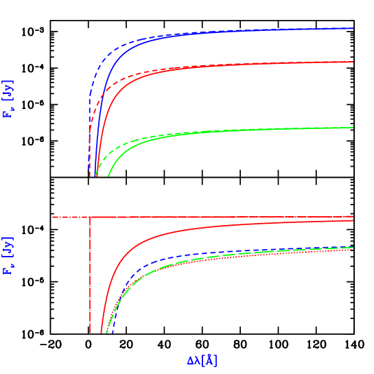
Figure 30: Expected spectral shape of the Ly$\alpha$ absorption trough due to intergalactic absorption in GRB afterglows (taken from BL04 ). The spectrum is presented in terms of the flux density $F_{\nu}$ versus relative observed wavelength $\Delta\lambda$, for a source redshift $z=7$ (assumed to be prior to the final reionization phase) and the typical halo mass $M=4\times 10^{8}M_{\odot}$ expected for GRB host galaxies that cool via atomic transitions. Top panel: Two examples for the predicted spectrum including IGM HI absorption (both resonant and damping wing), for host galaxies with (i) an age $t_{S}=10^{7}$ yr, a UV escape fraction $f_{\rm esc}=10\%$ and a Scalo initial mass function (IMF) in solid curves, or (ii) $t_{S}=10^{8}$ yr, $f_{\rm esc}=90\%$ and massive ($>100M_{\odot}$) Pop III stars in dashed curves. The observed time after the $\gamma$-ray trigger is one hour, one day, and ten days, from top to bottom, respectively. Bottom panel: Predicted spectra one day after a GRB for a host galaxy with $t_{S}=10^{7}$ yr, $f_{\rm esc}=10\%$ and a Scalo IMF. Shown is the unabsorbed GRB afterglow (dot-short dashed curve), the afterglow with resonant IGM absorption only (dot-long dashed curve), and the afterglow with full (resonant and damping wing) IGM absorption (solid curve). Also shown, with 1.7 magnitudes of extinction, are the afterglow with full IGM absorption (dotted curve), and attempts to reproduce this profile with a damped Ly$\alpha$ absorption system in the host galaxy (dashed curves). (Note, however, that damped absorption of this type could be suppressed by the ionizing effect of the afterglow UV radiation on the surrounding interstellar medium of its host galaxyPL98 .) Most importantly, the overall spectral shape of the Ly$\alpha$ trough carries precious information about the neutral fraction of the IGM at the source redshift; averaging over an ensemble of sources with similar redshifts can reduce ambiguities in the interpretation of each case due to particular local effects.

Although the nature of the central engine that powers the relativistic jets of GRBs is still unknown, recent evidence indicates that long-duration GRBs trace the formation of massive stars (e.g., T97 ; Wij98 ; BN00 ; Kul00 ; BKD02 ; Nat05 ) and in particular that long-duration GRBs are associated with Type Ib/c supernovae Sta03 . Since the first stars in the Universe are predicted to be predominantly massive ABN02 ; BCL02 ; Bromm , their death might give rise to large numbers of GRBs at high redshifts. In contrast to quasars of comparable brightness, GRB afterglows are short-lived and release $\sim 10$ orders of magnitude less energy into the surrounding IGM. Beyond the scale of their host galaxy, they have a negligible effect on their cosmological environment. Consequently, they are ideal probes of the IGM during the reionization epoch. Their rest-frame UV spectra can be used to probe the ionization state of the IGM through the spectral shape of the Gunn-Peterson (Ly$\alpha$) absorption trough, or its metal enrichment history through the intersection of enriched bubbles of supernova (SN) ejecta from early galaxies FL03 . Afterglows that are unusually bright ($>10$mJy) at radio frequencies should also show a detectable forest of 21 cm absorption lines due to enhanced HI column densities in sheets, filaments, and collapsed minihalos within the IGM Carilli04 ; FL02 .

Another advantage of GRB afterglows is that once they fade away, one may search for their host galaxies. Hence, GRBs may serve as signposts of the earliest dwarf galaxies that are otherwise too faint or rare on their own for a dedicated search to find them. Detection of metal absorption lines from the host galaxy in the afterglow spectrum, offers an unusual opportunity to study the physical conditions (temperature, metallicity, ionization state, and kinematics) in the interstellar medium of these high-redshift galaxies. As Figure 30 indicates, damped Ly$\alpha$ absorption within the host galaxy may mask the clear signature of the Gunn-Peterson trough in some galaxies BL04 . A small fraction ($\sim 10$) of the GRB afterglows are expected to originate at redshifts $z>5$ BL02 ; BL06 . This subset of afterglows can be selected photometrically using a small telescope, based on the Ly$\alpha$ break at a wavelength of $1.216\,\mu{\rm m}\,[(1+z)/10]$, caused by intergalactic HI absorption. The challenge in the upcoming years will be to follow-up on these candidates spectroscopically, using a large (10-meter class) telescope. GRB afterglows are likely to revolutionize observational cosmology and replace traditional sources like quasars, as probes of the IGM at $z>5$. The near future promises to be exciting for GRB astronomy as well as for studies of the high-redshift Universe.

It is of great importance to constrain the Pop III star formation mode, and in particular to determine down to which redshift it continues to be prominent. The extent of the Pop III star formation will affect models of the initial stages of reionization (e.g., WL03 ; CFW03 ; Sok04 ; YBH04 ; ABS06 ) and metal enrichment (e.g., MBH03 ; FL03 ; FL05 ; Sch03 ; SSR04 ), and will determine whether planned surveys will be able to effectively probe Pop III stars (e.g., Sca05 ). The constraints on Pop III star formation will also determine whether the first stars could have contributed a significant fraction to the cosmic near-IR background (e.g., SBK02 ; SF03 ; Kas05 ; MS05 ; DAK05 ). To constrain high-redshift star formation from GRB observations, one has to address two major questions:

(1) What is the signature of GRBs that originate in metal-free, Pop III progenitors? Simply knowing that a given GRB came from a high redshift is not sufficient to reach a definite conclusion as to the nature of the progenitor. Pregalactic metal enrichment was likely inhomogeneous, and we expect normal Pop I and II stars to exist in galaxies that were already metal-enriched at these high redshifts BL06 . Pop III and Pop I/II star formation is thus predicted to have occurred concurrently at $z>5$. How is the predicted high mass-scale for Pop III stars reflected in the observational signature of the resulting GRBs? Preliminary results from numerical simulations of Pop III star formation indicate that circumburst densities are systematically higher in Pop III environments. GRB afterglows will then be much brighter than for conventional GRBs. In addition, due to the systematically increased progenitor masses, the Pop III distribution may be biased toward long-duration events.

(2) The modelling of Pop III cosmic star formation histories has a number of free parameters, such as the star formation efficiency and the strength of the chemical feedback. The latter refers to the timescale for, and spatial extent of, the distribution of the first heavy elements that were produced inside of Pop III stars, and subsequently dispersed into the IGM by supernova blast waves. Comparing with theoretical GRB redshift distributions one can use the GRB redshift distribution observed by Swift to calibrate the free model parameters. In particular, one can use this strategy to measure the redshift where Pop III star formation terminates.

Figure 31: Theoretical prediction for the comoving star formation rate (SFR) in units of $M_{\odot}$ yr^-1 Mpc^-3, as a function of redshift (from BL06 ). We assume that cooling in primordial gas is due to atomic hydrogen only, a star formation efficiency of $\eta_{\ast}=10\%$, and reionization beginning at $z_{\rm reion}\approx 17$. Solid line: Total comoving SFR. Dotted lines: Contribution to the total SFR from Pop I/II and Pop III for the case of weak chemical feedback. Dashed lines: Contribution to the total SFR from Pop I/II and Pop III for the case of strong chemical feedback. Pop III star formation is restricted to high redshifts, but extends over a significant range, $\Delta z\sim 10-15$.

Figures 31 and 32 illustrate these issues (based on BL06 ). Figure 32 leads to the robust expectation that $\sim 10$% of all Swift bursts should originate at $z>5$. This prediction is based on the contribution from Population I/II stars which are known to exist even at these high redshifts. Additional GRBs could be triggered by Pop III stars, with a highly uncertain efficiency. Assuming that long-duration GRBs are produced by the collapsar mechanism, a Pop III star with a close binary companion provides a plausible GRB progenitor. The Pop III GRB efficiency, reflecting the probability of forming sufficiently close and massive binary systems, to lie between zero (if tight Pop III binaries do not exist) and $\sim 10$ times the empirically inferred value for Population I/II (due to the increased fraction of black hole forming progenitors among the massive Pop III stars).

A key ingredient in determining the underlying star formation history from the observed GRB redshift distribution is the GRB luminosity function, which is only poorly constrained at present. The improved statistics provided by Swift will enable the construction of an empirical luminosity function. With an improved luminosity function it would be possible to re-calibrate the theoretical prediction in Figure 2 more reliably.

Figure 32: Predicted GRB rate to be observed by Swift (from BL06 ). Shown is the observed number of bursts per year, $dN_{\rm GRB}^{\rm obs}/d\ln(1+z)$, as a function of redshift. All rates are calculated with a constant GRB efficiency, $\eta_{\rm GRB}\simeq 2\times 10^{-9}$ bursts $M_{\odot}^{-1}$, using the cosmic SFRs from Fig. 31. Dotted lines: Contribution to the observed GRB rate from Pop I/II and Pop III for the case of weak chemical feedback. Dashed lines: Contribution to the GRB rate from Pop I/II and Pop III for the case of strong chemical feedback. Filled circle: GRB rate from Pop III stars if these were responsible for reionizing the Universe at $z\sim 17$.

In order to predict the observational signature of high-redshift GRBs, it is important to know the properties of the GRB host systems. Within variants of the popular CDM model for structure formation, where small objects form first and subsequently merge to build up more massive ones, the first stars are predicted to form at $z\sim 20$–$30$ in minihalos of total mass (dark matter plus gas) $\sim 10^{6}M_{\odot}$ Teg97 ; BL01 ; YBH04 . These objects are the sites for the formation of the first stars, and thus are the potential hosts of the highest-redshift GRBs. What is the environment in which the earliest GRBs and their afterglows did occur? This problem breaks down into two related questions: (i) what type of stars (in terms of mass, metallicity, and clustering properties) will form in each minihalo?, and (ii) how will the ionizing radiation from each star modify the density structure of the surrounding gas? These two questions are fundamentally intertwined. The ionizing photon production strongly depends on the stellar mass, which in turn is determined by how the accretion flow onto the growing protostar proceeds under the influence of this radiation field. In other words, the assembly of the Population III stars and the development of an HII region around them proceed simultaneously, and affect each other. As a preliminary illustration, Figure 27 describes the photo-evaporation as a self-similar champagne flow Shu02 with parameters appropriate for the Pop III case.

Figure 33: Effect of photoheating from a Population III star on the density profile in a high-redshift minihalo (from BrL06 ). The curves, labeled by the time after the onset of the central point source, are calculated according to a self-similar model for the expansion of an HII region. Numerical simulations closely conform to this analytical behavior. Notice that the central density is significantly reduced by the end of the life of a massive star, and that a central core has developed where the density is constant.

Notice that the central density is significantly reduced by the end of the life of a massive star, and that a central core has developed where the density is nearly constant. Such a flat density profile is markedly different from that created by stellar winds ($\rho\propto r^{-2}$). Winds, and consequently mass-loss, may not be important for massive Population III stars BHW01 ; K02 , and such a flat density profile may be characteristic of GRBs that originate from metal-free Population III progenitors.

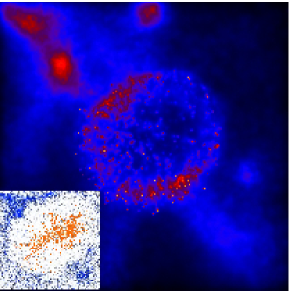
Figure 34: Supernova explosion in the high-redshift Universe (from BYH03 ). The snapshot is taken $\sim 10^{6}$ yr after the explosion with total energy $E_{\rm SN}\simeq 10^{53}$ ergs. We show the projected gas density within a box of linear size 1 kpc. The SN bubble has expanded to a radius of $\sim 200$ pc, having evacuated most of the gas in the minihalo. Inset: Distribution of metals. The stellar ejecta (gray dots) trace the metals and are embedded in pristine metal-poor gas (black dots).

The first galaxies may be surrounded by a shell of highly enriched material that was carried out in a SN-driven wind (see Fig. 34). A GRB in that galaxy may show strong absorption lines at a velocity separation associated with the wind velocity. Simulating these winds and calculating the absorption profile in the featureless spectrum of a GRB afterglow, will allow us to use the observed spectra of high-$z$ GRBs and directly probe the degree of metal enrichment in the vicinity of the first star forming regions (see FL03 for a semi-analytic treatment).

As the early afterglow radiation propagates through the interstellar environment of the GRB, it will likely modify the gas properties close to the source; these changes could in turn be noticed as time-dependent spectral features in the spectrum of the afterglow and used to derive the properties of the gas cloud (density, metal abundance, and size). The UV afterglow radiation can induce detectable changes to the interstellar absorption features of the host galaxy PL98 ; dust destruction could have occurred due to the GRB X-rays WD00 ; FKR01 , and molecules could have been destroyed near the GRB source DH02 . Quantitatively, all of the effects mentioned above strongly depend on the exact properties of the gas in the host system.

Most studies to date have assumed a constant efficiency of forming GRBs per unit mass of stars. This simplifying assumption could lead, under different circumstances, to an overestimation or an underestimation of the frequency of GRBs. Metal-free stars are thought to be massive ABN02 ; BCL02 and their extended envelopes may suppress the emergence of relativistic jets out of their surface (even if such jets are produced through the collapse of their core to a spinning black hole). On the other hand, low-metallicity stars are expected to have weak winds with little angular momentum loss during their evolution, and so they may preferentially yield rotating central configurations that make GRB jets after core collapse.

What kind of metal-free, Pop III progenitor stars may lead to GRBs? Long-duration GRBs appear to be associated with Type Ib/c supernovae Sta03 , namely progenitor massive stars that have lost their hydrogen envelope. This requirement is explained theoretically in the collapsar model, in which the relativistic jets produced by core collapse to a black hole are unable to emerge relativistically out of the stellar surface if the hydrogen envelope is retained MWH01 . The question then arises as to whether the lack of metal line-opacity that is essential for radiation-driven winds in metal-rich stars, would make a Pop III star retain its hydrogen envelope, thus quenching any relativistic jets and GRBs.

Aside from mass transfer in a binary system, individual Pop III stars could lose their hydrogen envelope due to either: (i) violent pulsations, particularly in the mass range $100$–$140M_{\odot}$, or (ii) a wind driven by helium lines. The outer stellar layers are in a state where gravity only marginally exceeds radiation pressure due to electron-scattering (Thomson) opacity. Adding the small, but still non-negligible contribution from the bound-free opacity provided by singly-ionized helium, may be able to unbind the atmospheric gas. Therefore, mass-loss might occur even in the absence of dust or any heavy elements.

5.4 Emission Spectrum of Metal-Free Stars

The evolution of metal-free (Population III) stars is qualitatively different from that of enriched (Population I and II) stars. In the absence of the catalysts necessary for the operation of the CNO cycle, nuclear burning does not proceed in the standard way. At first, hydrogen burning can only occur via the inefficient PP chain. To provide the necessary luminosity, the star has to reach very high central temperatures ($T_{c}\simeq 10^{8.1}$ K). These temperatures are high enough for the spontaneous turn-on of helium burning via the triple-$\alpha$ process. After a brief initial period of triple-$\alpha$ burning, a trace amount of heavy elements forms. Subsequently, the star follows the CNO cycle. In constructing main-sequence models, it is customary to assume that a trace mass fraction of metals ($Z\sim 10^{-9}$) is already present in the star (El Eid 1983 EFO83 ; Castellani et al. 1983 CCT83 ).

Figures 35 and 36 show the luminosity $L$ vs. effective temperature $T$ for zero-age main sequence stars in the mass ranges of $2$–$90M_{\odot}$ (Fig. 35) and $100$–$1000M_{\odot}$ (Fig. 36). Note that above $\sim 100M_{\odot}$ the effective temperature is roughly constant, $T_{\rm eff}\sim 10^{5}$K, implying that the spectrum is independent of the mass distribution of the stars in this regime (Bromm, Kudritzky, & Loeb 2001 BKL2001 ). As is evident from these figures (see also Tumlinson & Shull 2000 TS00 ), both the effective temperature and the ionizing power of metal-free (Pop III) stars are substantially larger than those of metal-rich (Pop I) stars. Metal-free stars with masses $>20M_{\odot}$ emit between $10^{47}$ and $10^{48}$ H I and He I ionizing photons per second per solar mass of stars, where the lower value applies to stars of $\sim 20M_{\odot}$ and the upper value applies to stars of $>100M_{\odot}$ (see Tumlinson & Shull 2000 TS00 and Bromm et al. 2001 BKL2001 for more details). Over a lifetime of $\sim 3\times 10^{6}$ years these massive stars produce $10^{4}$–$10^{5}$ ionizing photons per stellar baryon. However, this powerful UV emission is suppressed as soon as the interstellar medium out of which new stars form is enriched by trace amounts of metals. Even though the collapsed fraction of baryons is small at the epoch of reionization, it is likely that most of the stars responsible for the reionization of the Universe formed out of enriched gas.

Figure 35: Luminosity vs. effective temperature for zero-age main sequences stars in the mass range of $2$–$90M_{\odot}$ (from Tumlinson & Shull 2000 TS00 ). The curves show Pop I ($Z_{\odot}$ = 0.02) and Pop III stars of mass 2, 5, 8, 10, 15, 20, 25, 30, 35, 40, 50, 60, 70, 80, and 90 $M_{\odot}$. The diamonds mark decades in metallicity in the approach to $Z=0$ from 10^-2 down to 10^-5 at 2 $M_{\odot}$, down to 10^-10 at 15 $M_{\odot}$, and down to 10^-13 at 90 $M_{\odot}$. The dashed line along the Pop III ZAMS assumes pure H-He composition, while the solid line (on the left) marks the upper MS with $Z_{\rm C}=10^{-10}$ for the $M\geq 15$ $M_{\odot}$ models. Squares mark the points corresponding to pre-enriched evolutionary models from El Eid et al. (1983) EFO83 at 80 $M_{\odot}$ and from Castellani et al. (1983) CCT83 for 25 $M_{\odot}$.

Figure 36: Same as Figure 35 but for very massive stars above $100M_{\odot}$ (from Bromm, Kudritzki, & Loeb 2001 BKL2001 ). Left solid line: Pop III zero-age main sequence (ZAMS). Right solid line: Pop I ZAMS. In each case, stellar luminosity (in $L_{\odot}$) is plotted vs. effective temperature (in K). Diamond-shaped symbols: Stellar masses along the sequence, from $100M_{\odot}$ (bottom) to $1000M_{\odot}$ (top) in increments of $100M_{\odot}$. The Pop III ZAMS is systematically shifted to higher effective temperature, with a value of $\sim 10^{5}$ K which is approximately independent of mass. The luminosities, on the other hand, are almost identical in the two cases.

Will it be possible to infer the initial mass function (IMF) of the first stars from spectroscopic observations of the first galaxies? Figure 37 compares the observed spectrum from a Salpeter IMF ($dN_{\star}/dM\propto M^{-2.35}$) and a heavy IMF (with all stars more massive than $100M_{\odot}$) for a galaxy at $z_{s}=10$. The latter case follows from the assumption that each of the dense clumps in the simulations described in the previous section ends up as a single star with no significant fragmentation or mass loss. The difference between the plotted spectra cannot be confused with simple reddening due to normal dust. Another distinguishing feature of the IMF is the expected flux in the hydrogen and helium recombination lines, such as Ly$\alpha$ and He II 1640 Å, from the interstellar medium surrounding these stars. We discuss this next.

Figure 37: Comparison of the predicted flux from a Pop III star cluster at $z_{s}=10$ for a Salpeter IMF (Tumlinson & Shull 2000 TS00 ) and a massive IMF (Bromm et al. 2001 BKL2001 ). Plotted is the observed flux (in nJy per $10^{6}M_{\odot}$ of stars) vs. observed wavelength (in $\mu$m) for a flat Universe with $\Omega_{\Lambda}=0.7$ and $h=0.65$. Solid line: The case of a heavy IMF. Dotted line: The fiducial case of a standard Salpeter IMF. The cutoff below $\lambda_{obs}=1216\mbox{\,\AA\,}(1+z_{s})=1.34\mu$m is due to complete Gunn-Peterson absorption (which is artificially assumed to be sharp). Clearly, for the same total stellar mass, the observable flux is larger by an order of magnitude for stars which are biased towards having masses $>100M_{\odot}\,$.

5.5 Emission of Recombination Lines from the First Galaxies

The hard UV emission from a star cluster or a quasar at high redshift is likely reprocessed by the surrounding interstellar medium, producing very strong recombination lines of hydrogen and helium (Oh 1999 Oh99 ; Tumlinson & Shull 2000 TS00 ; see also Baltz, Gnedin & Silk 1998 Baltz98 ). We define $\dot{N}_{\rm ion}$ to be the production rate of ionizing photons by the source. The emitted luminosity $L_{\rm line}^{\rm em}$ per unit stellar mass in a particular recombination line is then estimated to be

$$L_{\rm line}^{\rm em}=p_{\rm line}^{\rm em}h\nu\dot{N}_{\rm ion}(1-p^{\rm esc}_{\rm cont})p^{\rm esc}_{\rm line}\mbox{\ \ \ ,}$$ (117)

where $p_{\rm line}^{\rm em}$ is the probability that a recombination leads to the emission of a photon in the corresponding line, $\nu$ is the frequency of the line and $p^{\rm esc}_{\rm cont}$ and $p^{\rm esc}_{\rm line}$ are the escape probabilities for the ionizing photons and the line photons, respectively. It is natural to assume that the stellar cluster is surrounded by a finite H II region, and hence that $p^{\rm esc}_{\rm cont}$ is close to zero WL00 ; RS00 . In addition, $p^{\rm esc}_{\rm line}$ is likely close to unity in the H II region, due to the lack of dust in the ambient metal-free gas. Although the emitted line photons may be scattered by neutral gas, they diffuse out to the observer and in the end survive if the gas is dust free. Thus, for simplicity, we adopt a value of unity for $p^{\rm esc}_{\rm line}$.

As a particular example we consider case B recombination which yields $p_{\rm line}^{\rm em}$ of about 0.65 and 0.47 for the Ly${\alpha}$ and He II 1640 Å lines, respectively. These numbers correspond to an electron temperature of $\sim 3\times 10^{4}$K and an electron density of $\sim 10^{2}-10^{3}$ cm^-3 inside the H II region SH95 . For example, we consider the extreme and most favorable case of metal-free stars all of which are more massive than $\sim 100M_{\odot}$. In this case $L_{\rm line}^{\rm em}=1.7\times 10^{37}$ and $2.2\times 10^{36}$ erg s${}^{-1}M_{\odot}^{-1}$ for the recombination luminosities of Ly$\alpha$ and He II 1640 Å per stellar mass BKL2001 . A cluster of $10^{6}M_{\odot}$ in such stars would then produce 4.4 and 0.6 $\times 10^{9}L_{\odot}$ in the Ly$\alpha$ and He II 1640 Å lines. Comparably-high luminosities would be produced in other recombination lines at longer wavelengths, such as He II 4686 Å and H$\alpha$ Oh99 ; OHR00 .

The rest–frame equivalent width of the above emission lines measured against the stellar continuum of the embedded star cluster at the line wavelengths is given by

$$W_{\lambda}=\left(\frac{L_{\rm line}^{\rm em}}{L_{\lambda}}\right)\mbox{\ \ \ ,}$$ (118)

where $L_{\lambda}$ is the spectral luminosity per unit wavelength of the stars at the line resonance. The extreme case of metal-free stars which are more massive than $100M_{\odot}$ yields a spectral luminosity per unit frequency $L_{\nu}=2.7\times 10^{21}$ and $1.8\times 10^{21}$ erg s^-1 Hz${}^{-1}M_{\odot}^{-1}$ at the corresponding wavelengths BKL2001 . Converting to $L_{\lambda}$, this yields rest-frame equivalent widths of $W_{\lambda}$ = 3100 Å and 1100 Å for Ly$\alpha$ and He II 1640 Å , respectively. These extreme emission equivalent widths are more than an order of magnitude larger than the expectation for a normal cluster of hot metal-free stars with the same total mass and a Salpeter IMF under the same assumptions concerning the escape probabilities and recombination Kud00 . The equivalent widths are, of course, larger by a factor of $(1+z_{s})$ in the observer frame. Extremely strong recombination lines, such as Ly$\alpha$ and He II 1640 Å, are therefore expected to be an additional spectral signature that is unique to very massive stars in the early Universe. The strong recombination lines from the first luminous objects are potentially detectable with JWST OHR00 .

6 Supermassive Black holes

6.1 The Principle of Self-Regulation

The fossil record in the present-day Universe indicates that every bulged galaxy hosts a supermassive black hole (BH) at its center Kor03 . This conclusion is derived from a variety of techniques which probe the dynamics of stars and gas in galactic nuclei. The inferred BHs are dormant or faint most of the time, but ocassionally flash in a short burst of radiation that lasts for a small fraction of the Hubble time. The short duty cycle acounts for the fact that bright quasars are much less abundant than their host galaxies, but it begs the more fundamental question: why is the quasar activity so brief? A natural explanation is that quasars are suicidal, namely the energy output from the BHs regulates their own growth.

Supermassive BHs make up a small fraction, $<10^{-3}$, of the total mass in their host galaxies, and so their direct dynamical impact is limited to the central star distribution where their gravitational influence dominates. Dynamical friction on the background stars keeps the BH close to the center. Random fluctuations in the distribution of stars induces a Brownian motion of the BH. This motion can be decribed by the same Langevin equation that captures the motion of a massive dust particle as it responds to random kicks from the much lighter molecules of air around it Cha02 . The characteristic speed by which the BH wanders around the center is small, $\sim(m_{\star}/M_{\rm BH})^{1/2}\sigma_{\star}$, where $m_{\star}$ and $M_{\rm BH}$ are the masses of a single star and the BH, respectively, and $\sigma_{\star}$ is the stellar velocity dispersion. Since the random force fluctuates on a dynamical time, the BH wanders across a region that is smaller by a factor of $\sim(m_{\star}/M_{\rm BH})^{1/2}$ than the region traversed by the stars inducing the fluctuating force on it.

The dynamical insignificance of the BH on the global galactic scale is misleading. The gravitational binding energy per rest-mass energy of galaxies is of order $\sim(\sigma_{\star}/c)^{2}<10^{-6}$. Since BH are relativistic objects, the gravitational binding energy of material that feeds them amounts to a substantial fraction its rest mass energy. Even if the BH mass occupies a fraction as small as $\sim 10^{-4}$ of the baryonic mass in a galaxy, and only a percent of the accreted rest-mass energy leaks into the gaseous environment of the BH, this slight leakage can unbind the entire gas reservoir of the host galaxy! This order-of-magnitude estimate explains why quasars are short lived. As soon as the central BH accretes large quantities of gas so as to significantly increase its mass, it releases large amounts of energy that would suppress further accretion onto it. In short, the BH growth is self-regulated.

The principle of self-regulation naturally leads to a correlation between the final BH mass, $M_{\rm bh}$, and the depth of the gravitational potential well to which the surrounding gas is confined which can be characterized by the velocity dispersion of the associated stars, $\sim\sigma_{\star}^{2}$. Indeed such a correlation is observed in the present-day Universe Tre02 . The observed power-law relation between $M_{\rm bh}$ and $\sigma_{\star}$ can be generalized to a correlation between the BH mass and the circular velocity of the host halo, $v_{c}$ Fer02 , which in turn can be related to the halo mass, $M_{\rm halo}$, and redshift, $z$ WL03

$$M_{\rm bh}(M_{\rm halo},z) = \mbox{const}\times v_{c}^{5}$$ (119)

$$=\epsilon_{\rm o}M_{\rm halo}\left(\frac{M_{\rm halo}}{10^{12}M_{\odot}}\right)^{\frac{2}{3}}[\zeta(z)]^{\frac{5}{6}}(1+z)^{\frac{5}{2}},$$

where $\epsilon_{\rm o}\approx 10^{-5.7}$ is a constant, and as before $\zeta\equiv[(\Omega_{m}/\Omega_{m}^{z})(\Delta_{c}/18\pi^{2})]$, $\Omega_{m}^{z}\equiv[1+(\Omega_{\Lambda}/\Omega_{m})(1+z)^{-3}]^{-1}$, $\Delta_{c}=18\pi^{2}+82d-39d^{2}$, and $d=\Omega_{m}^{z}-1$. If quasars shine near their Eddington limit as suggested by observations of low and high-redshift quasars Flo03 ; Wil03 , then the above value of $\epsilon_{\rm o}$ implies that a fraction of $\sim 5$–$10\%$ of the energy released by the quasar over a galactic dynamical time needs to be captured in the surrounding galactic gas in order for the BH growth to be self-regulated WL03 .

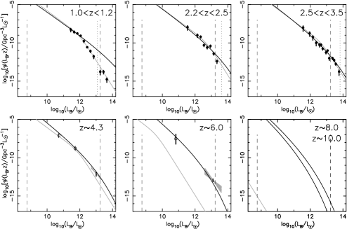
Figure 38: Comparison of the observed and model luminosity functions (from WL03 ). The data points at $z<4$ are summarized in Ref. Pei95 , while the light lines show the double power-law fit to the 2dF quasar luminosity function Boy00 . At $z\sim 4.3$ and $z\sim 6.0$ the data is from Refs. Fan01a . The grey regions show the 1-$\sigma$ range of logarithmic slope ($[-2.25,-3.75]$ at $z\sim 4.3$ and $[-1.6,-3.1]$ at $z\sim 6$), and the vertical bars show the uncertainty in the normalization. The open circles show data points converted from the X-ray luminosity function Bar03 of low luminosity quasars using the median quasar spectral energy distribution. In each panel the vertical dashed lines correspond to the Eddington luminosities of BHs bracketing the observed range of the $M_{\rm bh}$–$v_{\rm c}$ relation, and the vertical dotted line corresponds to a BH in a $10^{13.5}M_{\odot}$ galaxy.

With this interpretation, the $M_{\rm bh}$–$\sigma_{\star}$ relation reflects the limit introduced to the BH mass by self-regulation; deviations from this relation are inevitable during episodes of BH growth or as a result of mergers of galaxies that have no cold gas in them. A physical scatter around this upper envelope could also result from variations in the efficiency by which the released BH energy couples to the surrounding gas.

Various prescriptions for self-regulation were sketched by Silk & Rees Sil98 . These involve either energy or momentum-driven winds, where the latter type is a factor of $\sim v_{c}/c$  less efficient Beg04 ; Kin03 ; Mur04 . Wyithe & Loeb WL03 demonstrated that a particularly simple prescription for an energy-driven wind can reproduce the luminosity function of quasars out to highest measured redshift, $z\sim 6$ (see Figs. 38 and 40), as well as the observed clustering properties of quasars at $z\sim 3$ WLcl (see Fig. 41). The prescription postulates that: (i) self-regulation leads to the growth of $M_{\rm bh}$ up the redshift-independent limit as a function of $v_{c}$ in Eq. (119), for all galaxies throughout their evolution; and (ii) the growth of $M_{\rm bh}$ to the limiting mass in Eq. (119) occurs through halo merger episodes during which the BH shines at its Eddington luminosity (with the median quasar spectrum) over the dynamical time of its host galaxy, $t_{\rm dyn}$. This model has only one adjustable parameter, namely the fraction of the released quasar energy that couples to the surrounding gas in the host galaxy. This parameter can be fixed based on the $M_{\rm bh}$–$\sigma_{\star}$ relation in the local Universe Fer02 . It is remarkable that the combination of the above simple prescription and the standard $\Lambda$CDM cosmology for the evolution and merger rate of galaxy halos, lead to a satisfactory agreement with the rich data set on quasar evolution over cosmic history.

The cooling time of the heated gas is typically longer than its dynamical time and so the gas should expand into the galactic halo and escape the galaxy if its initial temperature exceeds the virial temperature of the galaxy WL03 . The quasar remains active during the dynamical time of the initial gas reservoir, $\sim 10^{7}$ years, and fades afterwards due to the dilution of this reservoir. Accretion is halted as soon as the quasar supplies the galactic gas with more than its binding energy. The BH growth may resume if the cold gas reservoir is replenished through a new merger.

Following the early analytic work, extensive numerical simulations by Springel, Hernquist, & Di Matteo (2005) SDH05 (see also Di Matteo et al. 2005 DSH05 ) demonstrated that galaxy mergers do produce the observed correlations between black hole mass and spheroid properties when a similar energy feedback is incorporated. Because of the limited resolution near the galaxy nucleus, these simulations adopt a simple prescription for the accretion flow that feeds the black hole. The actual feedback in reality may depend crucially on the geometry of this flow and the physical mechanism that couples the energy or momentum output of the quasar to the surrounding gas.

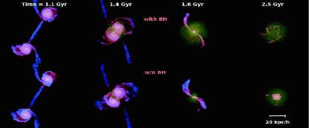
Figure 39: Simulation images of a merger of galaxies resulting in quasar activity that eventually shuts-off the accretion of gas onto the black hole (from Di Matteo et al. 2005 DSH05 ). The upper (lower) panels show a sequence of snapshots of the gas distribution during a merger with (without) feedback from a central black hole. The temperature of the gas is color coded.

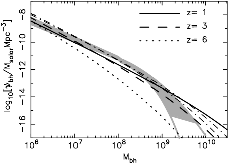
Figure 40: The comoving density of supermassive BHs per unit BH mass (from WL03 ). The grey region shows the estimate based on the observed velocity distribution function of galaxies in Ref. She03 and the $M_{\rm bh}$–$v_{c}$ relation in Eq. (119). The lower bound corresponds to the lower limit in density for the observed velocity function while the grey lines show the extrapolation to lower densities. We also show the mass function computed at $z=1$, 3 and 6 from the Press-Schechterps74 halo mass function and Eq. (119), as well as the mass function at $z\sim 2.35$ and $z\sim 3$ implied by the observed density of quasars and a quasar lifetime of order the dynamical time of the host galactic disk, $t_{\rm dyn}$ (dot-dashed lines).

Agreement between the predicted and observed correlation function of quasars (Fig. 41) is obtained only if the BH mass scales with redshift as in Eq. (119) and the quasar lifetime is of the order of the dynamical time of the host galactic disk WLcl ,

$$t_{\rm dyn}=10^{7}~{}[\xi(z)]^{-1/2}\left({1+z\over 3}\right)^{-3/2}~{}{\rm yr}.$$ (120)

This characterizes the timescale it takes low angular momentum gas to settle inwards and feed the black hole from across the galaxy before feedback sets in and suppresses additional infall. It also characterizes the timescale for establishing an outflow at the escape speed from the host spheroid.

The inflow of cold gas towards galaxy centers during the growth phase of the BH would naturally be accompanied by a burst of star formation. The fraction of gas that is not consumed by stars or ejected by supernovae, will continue to feed the BH. It is therefore not surprising that quasar and starburst activities co-exist in Ultra Luminous Infrared Galaxies Gen02 , and that all quasars show broad metal lines indicating a super-solar metallicity of the surrounding gas Ham03 . Applying a similar self-regulation principle to the stars, leads to the expectation WL03 ; Kau00 that the ratio between the mass of the BH and the mass in stars is independent of halo mass (as observed locally Mag98 ) but increases with redshift as $\propto\xi(z)^{1/2}(1+z)^{3/2}$. A consistent trend has indeed been inferred in an observed sample of gravitationally-lensed quasars Rix99 .

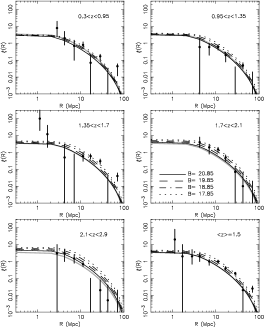
Figure 41: Predicted correlation function of quasars at various redshifts in comparison to the 2dF data Cro01 (from WLcl ). The dark lines show the correlation function predictions for quasars of various apparent B-band magnitudes. The 2dF limit is $B\sim 20.85$. The lower right panel shows data from entire 2dF sample in comparison to the theoretical prediction at the mean quasar redshift of $\langle z\rangle=1.5$. The $B=20.85$ prediction at this redshift is also shown by thick gray lines in the other panels to guide the eye. The predictions are based on the scaling $M_{\rm bh}\propto v_{c}^{5}$ in Eq. (119).

The upper mass of galaxies may also be regulated by the energy output from quasar activity. This would account for the fact that cooling flows are suppressed in present-day X-ray clusters Fab04 ; Boe02 ; OhS04 , and that massive BHs and stars in galactic bulges were already formed at $z\sim 2$. The quasars discovered by the Sloan Digital Sky Survey (SDSS) at $z\sim 6$ mark the early growth of the most massive BHs and galactic spheroids. The present-day abundance of galaxies capable of hosting BHs of mass $\sim 10^{9}M_{\odot}$ (based on Eq. 119) already existed at $z\sim 6$  Loe03 . At some epoch, the quasar energy output may have led to the extinction of cold gas in these galaxies and the suppression of further star formation in them, leading to an apparent “anti-hierarchical” mode of galaxy formation where massive spheroids formed early and did not make new stars at late times. In the course of subsequent merger events, the cores of the most massive spheroids acquired an envelope of collisionless matter in the form of already-formed stars or dark matter Loe03 , without the proportional accretion of cold gas into the central BH. The upper limit on the mass of the central BH and the mass of the spheroid is caused by the lack of cold gas and cooling flows in their X-ray halos. In the cores of cooling X-ray clusters, there is often an active central BH that supplies sufficient energy to compensate for the cooling of the gas Boe02 ; Fab04 ; Beg04 . The primary physical process by which this energy couples to the gas is still unknown.

Figure 42: The global influence of magnetized quasar outflows on the intergalactic medium (from Fur01 ). Upper Panel: Predicted volume filling fraction of magnetized quasar bubbles $F(z)$, as a function of redshift. Lower Panel: Ratio of normalized magnetic energy density, $\bar{u}_{B}/\epsilon_{-1}$, to the fiducial thermal energy density of the intergalactic medium $u_{fid}=3n(z)kT_{IGM}$, where $T_{IGM}=10^{4}~{}{\rm K}$, as a function of redshift (see Fur01 for more details). In each panel, the solid curves assume that the blast wave created by quasar ouflows is nearly (80%) adiabatic, and that the minimum halo mass of galaxies, $M_{h,min}$, is determined by atomic cooling before reionization and by suppression due to galactic infall afterwards (top curve), $M_{h,min}=10^{9}M_{\odot}$ (middle curve), and $M_{h,min}=10^{10}M_{\odot}$ (bottom curve). The dashed curve assumes a fully-radiative blast wave and fixes $M_{h,min}$ by the thresholds for atomic cooling and infall suppression. The vertical dotted line indicates the assumed redshift of complete reionization, $z_{r}=7$.

6.2 Feedback on Large Intergalactic Scales

Aside from affecting their host galaxy, quasars disturb their large-scale cosmological environment. Powerful quasar outflows are observed in the form of radio jets Beg84 or broad-absorption-line winds Bran03 . The amount of energy carried by these outflows is largely unknown, but could be comparable to the radiative output from the same quasars. Furlanetto & Loeb Fur01 have calculated the intergalactic volume filled by such outflows as a function of cosmic time (see Fig. 42). This volume is likely to contain magnetic fields and metals, providing a natural source for the observed magnetization of the metal-rich gas in X-ray clusters Kro01 and in galaxies Dal90 . The injection of energy by quasar outflows may also explain the deficit of Ly$\alpha$ absorption in the vicinity of Lyman-break galaxies Ade03 ; Cro02 and the required pre-heating in X-ray clusters Bor02 ; Boe02 .

Beyond the reach of their outflows, the brightest SDSS quasars at $z>6$ are inferred to have ionized exceedingly large regions of gas (tens of comoving Mpc) around them prior to global reionization (see Fig. 43 and Refs. WB1 ; WL04c ). Thus, quasars must have suppressed the faint-end of the galaxy luminosity function in these regions before the same occurred throughout the Universe. The recombination time is comparable to the Hubble time for the mean gas density at $z\sim 7$ and so ionized regions persist Oh03 on these large scales where inhomogeneities are small. The minimum galaxy mass is increased by at least an order of magnitude to a virial temperature of $\sim 10^{5}$K in these ionized regions BL01 . It would be particularly interesting to examine whether the faint end ($\sigma_{\star}<30{\rm km~{}s^{-1}}$) of the luminosity function of dwarf galaxies shows any moduluation on large-scales around rare massive BHs, such as M87.

To find the volume filling fraction of relic regions from $z\sim 6$, we consider a BH of mass $M_{\rm bh}\sim 3\times 10^{9}M_{\odot}$. We can estimate the comoving density of BHs directly from the observed quasar luminosity function and our estimate of quasar lifetime. At $z\sim 6$, quasars powered by $M_{\rm bh}\sim 3\times 10^{9}M_{\odot}$ BHs had a comoving density of $\sim 0.5\mbox{Gpc}^{-3}$WL03 . However, the Hubble time exceeds $t_{\rm dyn}$ by a factor of $\sim 2\times 10^{2}$ (reflecting the square root of the density contrast of cores of galaxies relative to the mean density of the Universe), so that the comoving density of the bubbles created by the $z\sim 6$ BHs is $\sim 10^{2}\mbox{Gpc}^{-3}$ (see Fig. 40). The density implies that the volume filling fraction of relic $z\sim 6$ regions is small, $<10\%$, and that the nearest BH that had $M_{\rm bh}\sim 3\times 10^{9}M_{\odot}$ at $z\sim 6$ (and could have been detected as an SDSS quasar then) should be at a distance $d_{\rm bh}\sim\left(4\pi/3\times 10^{2}\right)^{1/3}\mbox{Gpc}\sim 140\mbox{Mpc}$ which is almost an order-of-magnitude larger than the distance of M87, a galaxy known to possess a BH of this mass For94 .

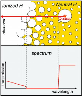
Figure 43: Quasars serve as probes of the end of reionization. The measured size of the HII regions around SDSS quasars can be used WL04b ; Mes04 to demonstrate that a significant fraction of the intergalactic hydrogen was neutral at $z\sim 6.3$ or else the inferred size of the quasar HII regions would have been much larger than observed (assuming typical quasar lifetimes Mar03 ). Also, quasars can be used to measure the redshift at which the intergalactic medium started to transmit Ly$\alpha$ photonsWB1 ; WL04c . The upper panel illustrates how the line-of-sight towards a quasar intersects this transition redshift. The resulting Ly$\alpha$ transmission of the intrinsic quasar spectrum is shown schematically in the lower panel.

What is the most massive BH that can be detected dynamically in a local galaxy redshift survey? SDSS probes a volume of $\sim 1\mbox{Gpc}^{3}$ out to a distance $\sim 30$ times that of M87. At the peak of quasar activity at $z\sim 3$, the density of the brightest quasars implies that there should be $\sim 100$ BHs with masses of $3\times 10^{10}M_{\odot}$ per $\mbox{Gpc}^{3}$, the nearest of which will be at a distance $d_{\rm bh}\sim 130\mbox{Mpc}$, or $\sim 7$ times the distance to M87. The radius of gravitational influence of the BH scales as $M_{\rm bh}/v_{\rm c}^{2}\propto M_{\rm bh}^{3/5}$. We find that for the nearest $3\times 10^{9}M_{\odot}$ and $3\times 10^{10}M_{\odot}$ BHs, the angular radius of influence should be similar. Thus, the dynamical signature of $\sim 3\times 10^{10}M_{\odot}$ BHs on their stellar host should be detectable.

6.3 What seeded the growth of the supermassive black holes?

The BHs powering the bright SDSS quasars possess a mass of a few $\times 10^{9}M_{\odot}$, and reside in galaxies with a velocity dispersion of $\sim 500{\rm km~{}s^{-1}}$nature . A quasar radiating at its Eddington limiting luminosity, $L_{E}=1.4\times 10^{46}~{}{\rm erg~{}s^{-1}}(M_{\rm bh}/10^{8}M_{\odot})$, with a radiative efficiency, $\epsilon_{\rm rad}=L_{E}/{\dot{M}}c^{2}$ would grow exponentially in mass as a function of time $t$, $M_{\rm bh}=M_{\rm seed}\exp\{t/t_{E}\}$ on a time scale, $t_{E}=4.1\times 10^{7}~{}{\rm yr}(\epsilon_{\rm rad}/0.1)$. Thus, the required growth time in units of the Hubble time $t_{\rm hubble}=9\times 10^{8}~{}{\rm yr}[(1+z)/7]^{-3/2}$ is

$${t_{\rm growth}\over t_{\rm hubble}}=0.7\left({\epsilon_{\rm rad}\over 10\%}\right)\left({1+z\over 7}\right)^{3/2}\ln\left({{M_{\rm bh}/10^{9}M_{\odot}}\over M_{\rm seed}/100M_{\odot}}\right)~{}.$$ (121)

The age of the Universe at $z\sim 6$ provides just sufficient time to grow an SDSS BH with $M_{\rm bh}\sim 10^{9}M_{\odot}$ out of a stellar mass seed with $\epsilon_{\rm rad}=10\%$ Hai01 . The growth time is shorter for smaller radiative efficiencies, as expected if the seed originates from the optically-thick collapse of a supermassive star (in which case $M_{\rm seed}$ in the logarithmic factor is also larger).

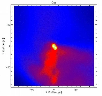
Figure 44: SPH simulation of the collapse of an early dwarf galaxy with a virial temperature just above the cooling threshold of atomic hydrogen and no H₂ (from Bro03 ). The image shows a snapshot of the gas density distribution at $z\approx 10$, indicating the formation of two compact objects near the center of the galaxy with masses of $2.2\times 10^{6}M_{\odot}$ and $3.1\times 10^{6}M_{\odot}$, respectively, and radii $<1$ pc. Sub-fragmentation into lower mass clumps is inhibited as long as molecular hydrogen is dissociated by a background UV flux. These circumstances lead to the formation of supermassive stars Loe94 that inevitably collapse and trigger the birth of supermassive black holes Loe94 ; Bau02 . The box size is 200 pc.

What was the mass of the initial BH seeds? Were they planted in early dwarf galaxies through the collapse of massive, metal free (Pop-III) stars (leading to $M_{\rm seed}$ of hundreds of solar masses) or through the collapse of even more massive, i.e. supermassive, stars Loe94 ?  Bromm & Loeb Bro03 have shown through a hydrodynamical simulation (see Fig. 44) that supermassive stars were likely to form in early galaxies at $z\sim 10$ in which the virial temperature was close to the cooling threshold of atomic hydrogen, $\sim 10^{4}$K. The gas in these galaxies condensed into massive $\sim 10^{6}M_{\odot}$ clumps (the progenitors of supermassive stars), rather than fragmenting into many small clumps (the progenitors of stars), as it does in environments that are much hotter than the cooling threshold. This formation channel requires that a galaxy be close to its cooling threshold and immersed in a UV background that dissociates molecular hydrogen in it. These requirements should make this channel sufficiently rare, so as not to overproduce the cosmic mass density of supermassive BH.

The minimum seed BH mass can be identified observationally through the detection of gravitational waves from BH binaries with Advanced LIGO WL04a or with LISA WL03b . Most of the mHz binary coalescence events originate at $z>7$ if the earliest galaxies included BHs that obey the $M_{\rm bh}$–$v_{c}$ relation in Eq. (119). The number of LISA sources per unit redshift per year should drop substantially after reionization, when the minimum mass of galaxies increased due to photo-ionization heating of the intergalactic medium. Studies of the highest redshift sources among the few hundred detectable events per year, will provide unique information about the physics and history of BH growth in galaxies Vol04 .

The early BH progenitors can also be detected as unresolved point sources, using the future James Webb Space Telescope (JWST). Unfortunately, the spectrum of metal-free massive and supermassive stars is the same, since their surface temperature $\sim 10^{5}$K is independent of mass BKL2001 . Hence, an unresolved cluster of massive early stars would show the same spectrum as a supermassive star of the same total mass.

It is difficult to ignore the possible environmental impact of quasars on anthropic selection. One may wonder whether it is not a coincidence that our Milky-Way Galaxy has a relatively modest BH mass of only a few million solar masses in that the energy output from a much more massive (e.g. $\sim 10^{9}M_{\odot}$) black hole would have disrupted the evolution of life on our planet. A proper calculation remains to be done (as in the context of nearby Gamma-Ray Bursts Sca02 ) in order to demonstrate any such link.

7 Radiative Feedback from the First Sources of Light

7.1 Escape of Ionizing Radiation from Galaxies

The intergalactic ionizing radiation field, a key ingredient in the development of reionization, is determined by the amount of ionizing radiation escaping from the host galaxies of stars and quasars. The value of the escape fraction as a function of redshift and galaxy mass remains a major uncertainty in all current studies, and could affect the cumulative radiation intensity by orders of magnitude at any given redshift. Gas within halos is far denser than the typical density of the IGM, and in general each halo is itself embedded within an overdense region, so the transfer of the ionizing radiation must be followed in the densest regions in the Universe. Reionization simulations are limited in resolution and often treat the sources of ionizing radiation and their immediate surroundings as unresolved point sources within the large-scale intergalactic medium (see, e.g., Gnedin 2000 g00 ). The escape fraction is highly sensitive to the three-dimensional distribution of the UV sources relative to the geometry of the absorbing gas within the host galaxy (which may allow escape routes for photons along particular directions but not others).

The escape of ionizing radiation ($h\nu>13.6$eV, $\lambda<912$ Å) from the disks of present-day galaxies has been studied in recent years in the context of explaining the extensive diffuse ionized gas layers observed above the disk in the Milky Way RTKMH95 and other galaxies Rand96 ; HWR99 . Theoretical models predict that of order 3–14% of the ionizing luminosity from O and B stars escapes the Milky Way disk DS94 ; DSF99 . A similar escape fraction of $f_{\rm esc}=6$% was determined by Bland-Hawthorn & Maloney (1999) BM99 based on H$\alpha$ measurements of the Magellanic Stream. From Hopkins Ultraviolet Telescope observations of four nearby starburst galaxies (Leitherer et al. 1995 LFHL95 ; Hurwitz, Jelinsky, & Dixon 1997 HJD97 ), the escape fraction was estimated to be in the range 3%$<f_{\rm esc}<57$%. If similar escape fractions characterize high redshift galaxies, then stars could have provided a major fraction of the background radiation that reionized the IGM MS96 ; Madau99 . However, the escape fraction from high-redshift galaxies, which formed when the Universe was much denser ($\rho\propto(1+z)^{3}$), may be significantly lower than that predicted by models ment to describe present-day galaxies. Current reionization calculations assume that galaxies are isotropic point sources of ionizing radiation and adopt escape fractions in the range $5\%<f_{\rm esc}<60\%$ g00 .

Clumping is known to have a significant effect on the penetration and escape of radiation from an inhomogeneous medium Boi90 ; WG96 ; Neufeld91 ; HS99 ; BFDA00 . The inclusion of clumpiness introduces several unknown parameters into the calculation, such as the number and overdensity of the clumps, and the spatial correlation between the clumps and the ionizing sources. An additional complication may arise from hydrodynamic feedback, whereby part of the gas mass is expelled from the disk by stellar winds and supernovae (§8).

Wood & Loeb (2000) WL00 used a three-dimensional radiation transfer code to calculate the steady-state escape fraction of ionizing photons from disk galaxies as a function of redshift and galaxy mass. The gaseous disks were assumed to be isothermal, with a sound speed $c_{s}\sim 10~{}{\rm km~{}s^{-1}}$, and radially exponential, with a scale-length based on the characteristic spin parameter and virial radius of their host halos. The corresponding temperature of $\sim 10^{4}$ K is typical for a gas which is continuousely heated by photo-ionization from stars. The sources of radiation were taken to be either stars embedded in the disk, or a central quasar. For stellar sources, the predicted increase in the disk density with redshift resulted in a strong decline of the escape fraction with increasing redshift. The situation is different for a central quasar. Due to its higher luminosity and central location, the quasar tends to produce an ionization channel in the surrounding disk through which much of its ionizing radiation escapes from the host. In a steady state, only recombinations in this ionization channel must be balanced by ionizations, while for stars there are many ionization channels produced by individual star-forming regions and the total recombination rate in these channels is very high. Escape fractions $>10\%$ were achieved for stars at $z\sim 10$ only if $\sim 90\%$ of the gas was expelled from the disks or if dense clumps removed the gas from the vast majority ($>80\%$) of the disk volume (see Fig. 45). This analysis applies only to halos with virial temperatures $>10^{4}$ K. Ricotti & Shull (2000) RS00 reached similar conclusions but for a quasi-spherical configuration of stars and gas. They demonstrated that the escape fraction is substantially higher in low-mass halos with a virial temperature $<10^{4}$ K. However, the formation of stars in such halos depends on their uncertain ability to cool via the efficient production of molecular hydrogen.

Figure 45: Escape fractions of stellar ionizing photons from a gaseous disk embedded within a $10^{10}M_{\odot}$ halo which have formed at $z=10$ (from Wood & Loeb 2000 WL00 ). The curves show three different cases of clumpiness within the disk. The volume filling factor refers to either the ionizing emissivity, the gas clumps, or both, depending on the case. The escape fraction is substantial ($>1\%$) only if the gas distribution is highly clumped.

The main uncertainty in the above predictions involves the distribution of the gas inside the host galaxy, as the gas is exposed to the radiation released by stars and the mechanical energy deposited by supernovae. Given the fundamental role played by the escape fraction, it is desirable to calibrate its value observationally. Steidel, Pettini, & Adelberger Ste00 reported a detection of significant Lyman continuum flux in the composite spectrum of 29 Lyman break galaxies (LBG) with redshifts in the range $z=3.40\pm 0.09$. They co-added the spectra of these galaxies in order to be able to measure the low flux. Another difficulty in the measurement comes from the need to separate the Lyman-limit break caused by the interstellar medium from that already produced in the stellar atmospheres. After correcting for intergalactic absorption, Steidel et al. Ste00 inferred a ratio between the emergent flux density at 1500Å  and 900Å  (rest frame) of $4.6\pm 1.0$. Taking into account the fact that the stellar spectrum should already have an intrinsic Lyman discontinuity of a factor of $\sim 3$–5, but that only $\sim 15$–$20\%$ of the 1500Å  photons escape from typical LBGs without being absorbed by dust (Pettini et al. 1998 PKSDAG98a ; Adelberger et al. 2000 Ade00 ), the inferred 900Å  escape fraction is $f_{\rm esc}\sim 10$–$20\%$. Although the galaxies in this sample were drawn from the bluest quartile of the LBG spectral energy distributions, the measurement implies that this quartile may itself dominate the hydrogen-ionizing background relative to quasars at $z\sim 3$.

7.2 Propagation of Ionization Fronts in the IGM

The radiation output from the first stars ionizes hydrogen in a growing volume, eventually encompassing almost the entire IGM within a single H II bubble. In the early stages of this process, each galaxy produces a distinct H II region, and only when the overall H II filling factor becomes significant do neighboring bubbles begin to overlap in large numbers, ushering in the “overlap phase” of reionization. Thus, the first goal of a model of reionization is to describe the initial stage, when each source produces an isolated expanding H II region.

We assume a spherical ionized volume $V$, separated from the surrounding neutral gas by a sharp ionization front. Indeed, in the case of a stellar ionizing spectrum, most ionizing photons are just above the hydrogen ionization threshold of 13.6 eV, where the absorption cross-section is high and a very thin layer of neutral hydrogen is sufficient to absorb all the ionizing photons. On the other hand, an ionizing source such as a quasar produces significant numbers of higher energy photons and results in a thicker transition region.

In the absence of recombinations, each hydrogen atom in the IGM would only have to be ionized once, and the ionized proper volume $V_{p}$ would simply be determined by

$$\bar{n}_{H}V_{p}=N_{\gamma}\ ,$$ (122)

where $\bar{n}_{H}$ is the mean number density of hydrogen and $N_{\gamma}$ is the total number of ionizing photons produced by the source. However, the increased density of the IGM at high redshift implies that recombinations cannot be neglected. Indeed, in the case of a steady ionizing source (and neglecting the cosmological expansion), a steady-state volume would be reached corresponding to the Strömgren sphere, with recombinations balancing ionizations:

$$\alpha_{B}\bar{n}_{H}^{2}V_{p}=\frac{d\,N_{\gamma}}{dt}\ ,$$ (123)

where the recombination rate depends on the square of the density and on the case B recombination coefficient $\alpha_{B}=2.6\times 10^{-13}$ cm³ s^-1 for hydrogen at $T=10^{4}$ K. The exact evolution for an expanding H II region, including a non-steady ionizing source, recombinations, and cosmological expansion, is given by (Shapiro & Giroux 1987 SG87 )

$$\bar{n}_{H}\left(\frac{dV_{p}}{dt}-3HV_{p}\right)=\frac{d\,N_{\gamma}}{dt}-\alpha_{B}\left<n_{H}^{2}\right>V_{p}\ .$$ (124)

In this equation, the mean density $\bar{n}_{H}$ varies with time as $1/a^{3}(t)$. A critical physical ingredient is the dependence of recombination on the square of the density. This means that if the IGM is not uniform, but instead the gas which is being ionized is mostly distributed in high-density clumps, then the recombination time is very short. This is often dealt with by introducing a volume-averaged clumping factor $C$ (in general time-dependent), defined by

$$C=\left<n_{H}^{2}\right>/\bar{n}_{H}^{2}\ .$$ (125)

If the ionized volume is large compared to the typical scale of clumping, so that many clumps are averaged over, then equation (124) can be solved by supplementing it with equation (125) and specifying $C$. Switching to the comoving volume $V$, the resulting equation is

$$\frac{dV}{dt}=\frac{1}{\bar{n}_{H}^{0}}\frac{d\,N_{\gamma}}{dt}-\alpha_{B}\frac{C}{a^{3}}\bar{n}_{H}^{0}V\ ,$$ (126)

where the present number density of hydrogen is

$$\bar{n}_{H}^{0}=1.88\times 10^{-7}\left(\frac{\Omega_{b}h^{2}}{0.022}\right)\ {\rm cm}^{-3}\ .$$ (127)

This number density is lower than the total number density of baryons $\bar{n}_{b}^{0}$ by a factor of $\sim 0.76$, corresponding to the primordial mass fraction of hydrogen. The solution for $V(t)$ (generalized from Shapiro & Giroux 1987 SG87 ) around a source which turns on at $t=t_{i}$ is

$$V(t)=\int_{t_{i}}^{t}\frac{1}{\bar{n}_{H}^{0}}\frac{d\,N_{\gamma}}{dt^{\prime}}\,e^{F(t^{\prime},t)}dt^{\prime}\ ,$$ (128)

where

$$F(t^{\prime},t)=-\alpha_{B}\bar{n}_{H}^{0}\int_{t^{\prime}}^{t}\frac{C(t^{\prime\prime})}{a^{3}(t^{\prime\prime})}\,dt^{\prime\prime}\ .$$ (129)

At high redshift (when $(1+z)\gg|{\Omega_{m}}^{-1}-1|$), the scale factor varies as

$$a(t)\simeq\left(\frac{3}{2}\sqrt{{\Omega_{m}}}H_{0}t\right)^{2/3}\ ,$$ (130)

and with the additional assumption of a constant $C$ the function $F$ simplifies as follows. Defining

$$f(t)=a(t)^{-3/2}\ ,$$ (131)

we derive

$$F(t^{\prime},t)=-\frac{2}{3}\frac{\alpha_{B}\bar{n}_{H}^{0}}{\sqrt{{\Omega_{m}}}H_{0}}\,C\left[f(t^{\prime})-f(t)\right]=-0.262\left[f(t^{\prime})-f(t)\right]\ ,$$ (132)

where the last equality assumes $C=10$ and our standard choice of cosmological parameters: ${\Omega_{m}}=0.3$, ${\Omega_{\Lambda}}=0.7$, and $\Omega_{b}=0.045$. Although this expression for $F(t^{\prime},t)$ is in general an accurate approximation at high redshift, in the particular case of the $\Lambda$CDM model (where ${\Omega_{m}}+{\Omega_{\Lambda}}=1$) we get the exact result by replacing equation (131) with

$$f(t)=\sqrt{\frac{1}{a^{3}}+\frac{1-{\Omega_{m}}}{{\Omega_{m}}}}\ .$$ (133)

The size of the resulting H II region depends on the halo which produces it. Consider a halo of total mass $M$ and baryon fraction $\Omega_{b}/{\Omega_{m}}$. To derive a rough estimate, we assume that baryons are incorporated into stars with an efficiency of $f_{\rm star}=10\%$, and that the escape fraction for the resulting ionizing radiation is also $f_{\rm esc}=10\%$. If the stellar IMF is similar to the one measured locally Sca98 , then $N_{\gamma}\approx 4000$ ionizing photons are produced per baryon in stars (for a metallicity equal to $1/20$ of the solar value). We define a parameter which gives the overall number of ionizations per baryon,

$$N_{\rm ion}\equiv N_{\gamma}\,f_{\rm star}\,f_{\rm esc}\ .$$ (134)

If we neglect recombinations then we obtain the maximum comoving radius of the region which the halo of mass $M$ can ionize,

$$r_{\rm max}=\left(\frac{3}{4\pi}\,\frac{N_{\gamma}}{\bar{n}_{H}^{0}}\right)^{1/3}=\left(\frac{3}{4\pi}\,\frac{N_{\rm ion}}{\bar{n}_{H}^{0}}\,\frac{\Omega_{b}}{{\Omega_{m}}}\,\frac{M}{m_{p}}\right)^{1/3}=680\,{\rm kpc}\left(\frac{N_{\rm ion}}{40}\,\frac{M}{10^{8}M_{\odot}}\right)^{1/3}\ ,$$ (135)

for our standard set of parameters. The actual radius never reaches this size if the recombination time is shorter than the lifetime of the ionizing source. For an instantaneous starburst with the Scalo (1998) Sca98 IMF, the production rate of ionizing photons can be approximated as

$$\frac{d\,N_{\gamma}}{dt}=\frac{\alpha-1}{\alpha}\frac{N_{\gamma}}{t_{s}}\times\left\{\begin{array}[]{ll}\ \ \,1&\mbox{if $t<t_{s}$,}\\ \left(\frac{t}{t_{s}}\right)^{-\alpha}&\mbox{otherwise,}\end{array}\right.$$ (136)

where $N_{\gamma}=4000$, $\alpha=4.5$, and the most massive stars fade away with the characteristic timescale $t_{s}=3\times 10^{6}$ yr. In figure 46 we show the time evolution of the volume ionized by such a source, with the volume shown in units of the maximum volume $V_{\rm max}$ which corresponds to $r_{\rm max}$ in equation (135). We consider a source turning on at $z=10$ (solid curves) or $z=15$ (dashed curves), with three cases for each: no recombinations, $C=1$, and $C=10$, in order from top to bottom (Note that the result is independent of redshift in the case of no recombinations). When recombinations are included, the volume rises and reaches close to $V_{\rm max}$ before dropping after the source turns off. At large $t$ recombinations stop due to the dropping density, and the volume approaches a constant value (although $V\ll V_{\rm max}$ at large $t$ if $C=10$).

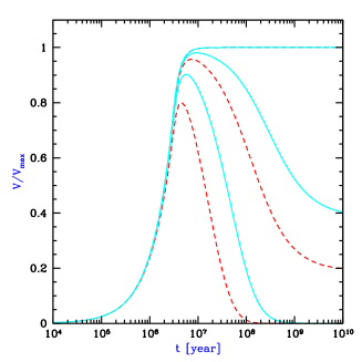
Figure 46: Expanding H II region around an isolated ionizing source. The comoving ionized volume $V$ is expressed in units of the maximum possible volume, $V_{\rm max}=4\pi r_{\rm max}^{3}/3$ [with $r_{\rm max}$ given in equation (135)], and the time is measured after an instantaneous starburst which produces ionizing photons according to equation (136). We consider a source turning on at $z=10$ (solid curves) or $z=15$ (dashed curves), with three cases for each: no recombinations, $C=1$, and $C=10$, in order from top to bottom. The no-recombination curve is identical for the different source redshifts.

We obtain a similar result for the size of the H II region around a galaxy if we consider a mini-quasar rather than stars. For the typical quasar spectrum (Elvis et al. 1994 ELV94 ), roughly 11,000 ionizing photons are produced per baryon incorporated into the black hole, assuming a radiative efficiency of $\sim 6\%$. The efficiency of incorporating the baryons in a galaxy into a central black hole is low ($<0.6\%$ in the local Universe, e.g. Magorrian et al. 1998 Mag98 ), but the escape fraction for quasars is likely to be close to unity, i.e., an order of magnitude higher than for stars (see previous sub-section). Thus, for every baryon in galaxies, up to $\sim 65$ ionizing photons may be produced by a central black hole and $\sim 40$ by stars, although both of these numbers for $N_{\rm ion}$ are highly uncertain. These numbers suggest that in either case the typical size of H II regions before reionization may be $<1$ Mpc or $\sim 10$ Mpc, depending on whether $10^{8}M_{\odot}$ halos or $10^{12}M_{\odot}$ halos dominate.

The ionization front around a bright transient source like a quasar expands at early times at nearly the speed of light. This occurs when the HII region is sufficiently small so that the production rate of ionizing photons by the central source exceeds their consumption rate by hydrogen atoms within this volume. It is straightforward to do the accounting for these rates (including recombinations) taking the light propagation delay into account. This was done by Wyithe & Loeb WL04b [see also White et al. (2003) WB1 ] who derived the general equation for the relativistic expansion of the comoving radius [$r=(1+z)r_{\rm p}$] of the quasar H II region in an IGM with a neutral filling fraction $x_{\rm HI}$ (fixed by other ionizing sources) as,

$$\frac{dr}{dt}=c(1+z)\left[\frac{\dot{N}_{\gamma}-\alpha_{\rm B}Cx_{\rm HI}\left(\bar{n}^{0}_{\rm H}\right)^{2}\left(1+z\right)^{3}\left({4\pi\over 3}r^{3}\right)}{\dot{N}_{\gamma}+4\pi r^{2}\left(1+z\right)cx_{\rm HI}\bar{n}^{0}_{\rm H}}\right],$$ (137)

where $c$ is the speed of light, $C$ is the clumping factor, $\alpha_{\rm B}=2.6\times 10^{-13}$cm³s^-1 is the case-B recombination coefficient at the characteristic temperature of $10^{4}$K, and $\dot{N}_{\gamma}$ is the rate of ionizing photons crossing a shell at the radius of the HII region at time $t$. Indeed, for $\dot{N}_{\gamma}\rightarrow\infty$ the propagation speed of the proper radius of the HII region $r_{p}=r/(1+z)$ approaches the speed of light in the above expression, $(dr_{p}/dt)\rightarrow c$. The actual size of the HII region along the line-of-sight to a quasar can be inferred from the extent of the spectral gap between the quasar’s rest-frame Ly$\alpha$ wavelength and the start of Ly$\alpha$ absorption by the IGM in the observed spectrum. Existing data from the SDSS quasars WL04b ; Mes04 ; Wy05 provide typical values of $r_{p}\sim 5$Mpc and indicate for plausible choices of the quasar lifetimes that $x_{\rm HI}>0.1$ at $z>6$. These ionized bubbles could be imaged directly by future 21cm maps of the regions around the highest-redshift quasars Tozzi ; WyLo ; WyBar .

The profile of the Ly$\alpha$ emission line of galaxies has also been suggested as a probe of the ionization state of the IGM Loeb_Rybicki ; Santos ; Haiman_Cen ; Haiman05 ; Madau_Rees ; Loeb_Hernquist ; Rhoads . If the IGM is neutral, then the damping wing of the Gunn-Peterson trough in equation (114) is modified since Ly$\alpha$ absorption starts only from the near edge of the ionized region along the line-of-sight to the source Haiman_Cen ; Madau_Rees . Rhoads & Malhotra Rhoads showed that the observed abundance of galaxies with Ly$\alpha$ emission at $z\sim 6.5$ indicates that a substantial fraction (tens of percent) of the IGM must be ionized in order to allow transmission of the observed Ly$\alpha$ photons. However, if these galaxies reside in groups, then galaxies with peculiar velocities away from the observer will preferentially Doppler-shift the emitted Ly$\alpha$ photons to the red wing of the Ly$\alpha$ resonance and reduce the depression of the line profile Loeb_Hernquist ; Haiman_Mesinger . Additional uncertainties in the intrinsic line profile based on the geometry and the stellar or gaseous contents of the source galaxy Loeb_Hernquist ; Santos , as well as the clustering of galaxies which ionize their immediate environment in groups WL04c ; Furlanetto_Hernquist , limits this method from reaching robust conclusions. Imaging of the expected halos of scattered Ly$\alpha$ radiation around galaxies embedded in a neutral IGM Loeb_Rybicki ; Rybicki_Loeb provide a more definitive test of the neutrality of the IGM, but is more challenging observationally.

7.3 Reionization of Hydrogen

In this section we summarize recent progress, both analytic and numerical, made toward elucidating the basic physics of reionization and the way in which the characteristics of reionization depend on the nature of the ionizing sources and on other input parameters of cosmological models.

The process of the reionization of hydrogen involves several distinct stages. The initial, “pre-overlap” stage (using the terminology of Gnedin g00 ) consists of individual ionizing sources turning on and ionizing their surroundings. The first galaxies form in the most massive halos at high redshift, and these halos are biased and are preferentially located in the highest-density regions. Thus the ionizing photons which escape from the galaxy itself (see §7.1) must then make their way through the surrounding high-density regions, which are characterized by a high recombination rate. Once they emerge, the ionization fronts propagate more easily into the low-density voids, leaving behind pockets of neutral, high-density gas. During this period the IGM is a two-phase medium characterized by highly ionized regions separated from neutral regions by ionization fronts. Furthermore, the ionizing intensity is very inhomogeneous even within the ionized regions, with the intensity determined by the distance from the nearest source and by the ionizing luminosity of this source.

The central, relatively rapid “overlap” phase of reionization begins when neighboring H II regions begin to overlap. Whenever two ionized bubbles are joined, each point inside their common boundary becomes exposed to ionizing photons from both sources. Therefore, the ionizing intensity inside H II regions rises rapidly, allowing those regions to expand into high-density gas which had previously recombined fast enough to remain neutral when the ionizing intensity had been low. Since each bubble coalescence accelerates the process of reionization, the overlap phase has the character of a phase transition and is expected to occur rapidly, over less than a Hubble time at the overlap redshift. By the end of this stage most regions in the IGM are able to see several unobscured sources, and therefore the ionizing intensity is much higher than before overlap and it is also much more homogeneous. An additional ingredient in the rapid overlap phase results from the fact that hierarchical structure formation models predict a galaxy formation rate that rises rapidly with time at the relevant redshift range. This process leads to a state in which the low-density IGM has been highly ionized and ionizing radiation reaches everywhere except for gas located inside self-shielded, high-density clouds. This marks the end of the overlap phase, and this important landmark is most often referred to as the ’moment of reionization’.

Some neutral gas does, however, remain in high-density structures which correspond to Lyman Limit systems and damped Ly$\alpha$ systems seen in absorption at lower redshifts. The high-density regions are gradually ionized as galaxy formation proceeds, and the mean ionizing intensity also grows with time. The ionizing intensity continues to grow and to become more uniform as an increasing number of ionizing sources is visible to every point in the IGM. This “post-overlap” phase continues indefinitely, since collapsed objects retain neutral gas even in the present Universe. The IGM does, however, reach another milestone at $z\sim 1.6$, the breakthrough redshift Mad99 . Below this redshift, all ionizing sources are visible to each other, while above this redshift absorption by the Ly$\alpha$ forest implies that only sources in a small redshift range are visible to a typical point in the IGM.

Semi-analytic models of the pre-overlap stage focus on the evolution of the H II filling factor, i.e., the fraction of the volume of the Universe which is filled by H II regions. We distinguish between the naive filling factor $F_{\rm H\ II}$ and the actual filling factor or porosity $Q_{\rm H\ II}$. The naive filling factor equals the number density of bubbles times the average volume of each, and it may exceed unity since when bubbles begin to overlap the overlapping volume is counted multiple times. However, as explained below, in the case of reionization the linearity of the physics means that $F_{\rm H\ II}$ is a very good approximation to $Q_{\rm H\ II}$ up to the end of the overlap phase of reionization.

The model of individual H II regions presented in the previous section can be used to understand the development of the total filling factor. Starting with equation (126), if we assume a common clumping factor $C$ for all H II regions then we can sum each term of the equation over all bubbles in a given large volume of the Universe, and then divide by this volume. Then $V$ is replaced by the filling factor and $N_{\gamma}$ by the total number of ionizing photons produced up to some time $t$, per unit volume. The latter quantity equals the mean number of ionizing photons per baryon times the mean density of baryons $\bar{n}_{b}$. Following the arguments leading to equation (135), we find that if we include only stars then

$$\frac{\bar{n}_{\gamma}}{\bar{n}_{b}}=N_{\rm ion}F_{\rm col}\ ,$$ (138)

where the collapse fraction $F_{\rm col}$ is the fraction of all the baryons in the Universe which are in galaxies, i.e., the fraction of gas which settles into halos and cools efficiently inside them. In writing equation (138) we are assuming instantaneous production of photons, i.e., that the timescale for the formation and evolution of the massive stars in a galaxy is short compared to the Hubble time at the formation redshift of the galaxy. In a model based on equation (126), the near-equality between $F_{\rm H\ II}$ and $Q_{\rm H\ II}$ results from the linearity of this equation. First, the total number of ionizations equals the total number of ionizing photons produced by stars, i.e., all ionizing photons contribute regardless of the spatial distribution of sources; and second, the total recombination rate is proportional to the total ionized volume, regardless of its topology. Thus, even if two or more bubbles overlap the model remains an accurate approximation for $Q_{\rm H\ II}$ (at least until $Q_{\rm H\ II}$ becomes nearly equal to 1). Note, however, that there still are a number of important simplifications in the model, including the assumption of a homogeneous (though possibly time-dependent) clumping factor, and the neglect of feedback whereby the formation of one galaxy may suppress further galaxy formation in neighboring regions. These complications are discussed in detail below and in §7.5 and §8.

Under these assumptions we convert equation (126), which describes individual H II regions, to an equation which statistically describes the transition from a neutral Universe to a fully ionized one (compare to Madau et al. 1999 Mad99 and Haiman & Loeb 1997 hl97 ):

$$\frac{dQ_{\rm H\ II}}{dt}=\frac{N_{\rm ion}}{0.76}\frac{dF_{\rm col}}{dt}-\alpha_{B}\frac{C}{a^{3}}\bar{n}_{H}^{0}Q_{\rm H\ II}\ ,$$ (139)

where we assumed a primordial mass fraction of hydrogen of 0.76. The solution (in analogy with equation (128)) is

$$Q_{\rm H\ II}(t)=\int_{0}^{t}\frac{N_{\rm ion}}{0.76}\frac{dF_{\rm col}}{dt^{\prime}}\,e^{F(t^{\prime},t)}dt^{\prime}\ ,$$ (140)

where $F(t^{\prime},t)$ is determined by equations (129)–( 133).

A simple estimate of the collapse fraction at high redshift is the mass fraction (given by equation (97) in the Press-Schechter model) in halos above the cooling threshold, which is the minimum mass of halos in which gas can cool efficiently. Assuming that only atomic cooling is effective during the redshift range of reionization, the minimum mass corresponds roughly to a halo of virial temperature $T_{\rm vir}=10^{4}$ K, which can be converted to a mass using equation (92). With this prescription we derive (for $N_{\rm ion}=40$) the reionization history shown in Fig. 47 for the case of a constant clumping factor $C$. The solid curves show $Q_{\rm H\ II}$ as a function of redshift for a clumping factor $C=0$ (no recombinations), $C=1$, $C=10$, and $C=30$, in order from left to right. Note that if $C\sim 1$ then recombinations are unimportant, but if $C>10$ then recombinations significantly delay the reionization redshift (for a fixed star-formation history). The dashed curve shows the collapse fraction $F_{\rm col}$ in this model. For comparison, the vertical dotted line shows the $z=5.8$ observational lower limit (Fan et al. 2000 f0 ) on the reionization redshift.

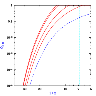
Figure 47: Semi-analytic calculation of the reionization of the IGM (for $N_{\rm ion}=40$), showing the redshift evolution of the filling factor $Q_{\rm H\ II}$. Solid curves show $Q_{\rm H\ II}$ for a clumping factor $C=0$ (no recombinations), $C=1$, $C=10$, and $C=30$, in order from left to right. The dashed curve shows the collapse fraction $F_{\rm col}$, and the vertical dotted line shows the $z=5.8$ observational lower limit (Fan et al. 2000 f0 ) on the reionization redshift.

Clearly, star-forming galaxies in CDM hierarchical models are capable of ionizing the Universe at $z\sim 6$–15 with reasonable parameter choices. This has been shown by a large number of theoretical, semi-analytic calculations fk94 ; sgb94 ; hl97 ; VS99 ; CO00 ; CFA00 ; Wyithe03 ; Cen03 ; Tumlinson04 as well as numerical simulations CO93 ; G097 ; g00 ; ANM99 ; RS99 ; Ciardi03 ; Sokasian03 ; Kohler05 ; Iliev05 . Similarly, if a small fraction ($<1\%$) of the gas in each galaxy accretes onto a central black hole, then the resulting mini-quasars are also able to reionize the Universe, as has also been shown using semi-analytic models fk94 ; HL98 ; VS99 ; Wyithe03 .

Although many models yield a reionization redshift around 7–12, the exact value depends on a number of uncertain parameters affecting both the source term and the recombination term in equation (139). The source parameters include the formation efficiency of stars and quasars and the escape fraction of ionizing photons produced by these sources. The formation efficiency of low mass galaxies may also be reduced by feedback from galactic outflows. These parameters affecting the sources are discussed elsewhere in this review (see §7.1, and 8). Even when the clumping is inhomogeneous, the recombination term in equation (139) is generally valid if $C$ is defined as in equation (125), where we take a global volume average of the square of the density inside ionized regions (since neutral regions do not contribute to the recombination rate). The resulting mean clumping factor depends on the density and clustering of sources, and on the distribution and topology of density fluctuations in the IGM. Furthermore, the source halos should tend to form in overdense regions, and the clumping factor is affected by this cross-correlation between the sources and the IGM density.

Miralda-Escudé, Haehnelt, & Rees (2000) MHR00 presented a simple model for the distribution of density fluctuations, and more generally they discussed the implications of inhomogeneous clumping during reionization. They noted that as ionized regions grow, they more easily extend into low-density regions, and they tend to leave behind high-density concentrations, with these neutral islands being ionized only at a later stage. They therefore argued that, since at high-redshift the collapse fraction is low, most of the high-density regions, which would dominate the clumping factor if they were ionized, will in fact remain neutral and occupy only a tiny fraction of the total volume. Thus, the development of reionization through the end of the overlap phase should occur almost exclusively in the low-density IGM, and the effective clumping factor during this time should be $\sim 1$, making recombinations relatively unimportant (see Fig. 47). Only in the post-reionization phase, Miralda-Escudé et al. (2000) MHR00 argued, do the high density clouds and filaments become gradually ionized as the mean ionizing intensity further increases.

The complexity of the process of reionization is illustrated by the numerical simulation of Gnedin g00 of stellar reionization (in $\Lambda$CDM with ${\Omega_{m}}=0.3$). This simulation uses a formulation of radiative transfer which relies on several rough approximations; although it does not include the effect of shadowing behind optically-thick clumps, it does include for each point in the IGM the effects of an estimated local optical depth around that point, plus a local optical depth around each ionizing source. This simulation helps to understand the advantages of the various theoretical approaches, while pointing to the complications which are not included in the simple models. Figures 48 and 49, taken from Figure 3 in g00 , show the state of the simulated Universe just before and just after the overlap phase, respectively. They show a thin (15 $h^{-1}$ comoving kpc) slice through the box, which is 4 $h^{-1}$ Mpc on a side, achieves a spatial resolution of $1h^{-1}$ kpc, and uses $128^{3}$ each of dark matter particles and baryonic particles (with each baryonic particle having a mass of $5\times 10^{5}M_{\odot}$). The figures show the redshift evolution of the mean ionizing intensity $J_{21}$ (upper right panel), and visually the logarithm of the neutral hydrogen fraction (upper left panel), the gas density (lower left panel), and the gas temperature (lower right panel). Note the obvious features resulting from the periodic boundary conditions assumed in the simulation. Also note that the intensity $J_{21}$ is defined as the intensity at the Lyman limit, expressed in units of $10^{-21}\,\mbox{ erg cm}^{-2}\mbox{ s}^{-1}\mbox{ sr}^{-1}\mbox{Hz}^{-1}$. For a given source emission, the intensity inside H II regions depends on absorption and radiative transfer through the IGM (e.g., Haardt & Madau 1996 HM96 ; Abel & Haehnelt 1999 AH99 )

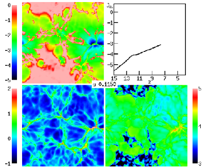
Figure 48: Visualization at $z=7.7$ of a numerical simulation of reionization, adopted from Figure 3c of g00 . The panels display the logarithm of the neutral hydrogen fraction (upper left), the gas density (lower left), and the gas temperature (lower right). Also shown is the redshift evolution of the logarithm of the mean ionizing intensity (upper right). Note the periodic boundary conditions.

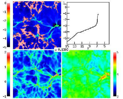
Figure 49: Visualization at $z=6.7$ of a numerical simulation of reionization, adopted from Figure 3e of g00 . The panels display the logarithm of the neutral hydrogen fraction (upper left), the gas density (lower left), and the gas temperature (lower right). Also shown is the redshift evolution of the logarithm of the mean ionizing intensity (upper right). Note the periodic boundary conditions.

Figure 48 shows the two-phase IGM at $z=7.7$, with ionized bubbles emanating from one main concentration of sources (located at the right edge of the image, vertically near the center; note the periodic boundary conditions). The bubbles are shown expanding into low density regions and beginning to overlap at the center of the image. The topology of ionized regions is clearly complex: While the ionized regions are analogous to islands in an ocean of neutral hydrogen, the islands themselves contain small lakes of dense neutral gas. One aspect which has not been included in theoretical models of clumping is clear from the figure. The sources themselves are located in the highest density regions (these being the sites where the earliest galaxies form) and must therefore ionize the gas in their immediate vicinity before the radiation can escape into the low density IGM. For this reason, the effective clumping factor is of order 100 in the simulation and also, by the overlap redshift, roughly ten ionizing photons have been produced per baryon. Figure 49 shows that by $z=6.7$ the low density regions have all become highly ionized along with a rapid increase in the ionizing intensity. The only neutral islands left are the highest density regions (compare the two panels on the left). However, we emphasize that the quantitative results of this simulation must be considered preliminary, since the effects of increased resolution and a more accurate treatment of radiative transfer are yet to be explored. Methods are being developed for incorporating a more complete treatment of radiative transfer into three dimensional cosmological simulations (e.g., ANM99 ; RS99 ; Ciardi03 ; Sokasian03 ; Kohler05 ; Iliev05 ).

Gnedin, Ferrara, & Zweibel (2000) GFZ00 investigated an additional effect of reionization. They showed that the Biermann battery in cosmological ionization fronts inevitably generates coherent magnetic fields of an amplitude $\sim 10^{-19}$ Gauss. These fields form as a result of the breakout of the ionization fronts from galaxies and their propagation through the H I filaments in the IGM. Although the fields are too small to directly affect galaxy formation, they could be the seeds for the magnetic fields observed in galaxies and X-ray clusters today.

If quasars contribute substantially to the ionizing intensity during reionization then several aspects of reionization are modified compared to the case of pure stellar reionization. First, the ionizing radiation emanates from a single, bright point-source inside each host galaxy, and can establish an escape route (H II funnel) more easily than in the case of stars which are smoothly distributed throughout the galaxy (§7.1). Second, the hard photons produced by a quasar penetrate deeper into the surrounding neutral gas, yielding a thicker ionization front. Finally, the quasar X-rays catalyze the formation of $H_{2}$ molecules and allow stars to keep forming in very small halos.

Oh (1999) Oh99 showed that star-forming regions may also produce significant X-rays at high redshift. The emission is due to inverse Compton scattering of CMB photons off relativistic electrons in the ejecta, as well as thermal emission by the hot supernova remnant. The spectrum expected from this process is even harder than for typical quasars, and the hard photons photoionize the IGM efficiently by repeated secondary ionizations. The radiation, characterized by roughly equal energy per logarithmic frequency interval, would produce a uniform ionizing intensity and lead to gradual ionization and heating of the entire IGM. Thus, if this source of emission is indeed effective at high redshift, it may have a crucial impact in changing the topology of reionization. Even if stars dominate the emission, the hardness of the ionizing spectrum depends on the initial mass function. At high redshift it may be biased toward massive, efficiently ionizing stars, but this remains very much uncertain.

Semi-analytic as well as numerical models of reionization depend on an extrapolation of hierarchical models to higher redshifts and lower-mass halos than the regime where the models have been compared to observations (see e.g. Wyithe03 ; Cen03 ; Tumlinson04 ). These models have the advantage that they are based on the current CDM paradigm which is supported by a variety of observations of large-scale structure, galaxy clustering, and the CMB. The disadvantage is that the properties of high-redshift galaxies are derived from those of their host halos by prescriptions which are based on low redshift observations, and these prescriptions will only be tested once abundant data is available on galaxies which formed during the reionization era (see Wyithe03 for the sensitivity of the results to model parameters). An alternative approach to analyzing the possible ionizing sources which brought about reionization is to extrapolate from the observed populations of galaxies and quasars at currently accessible redshifts. This has been attempted, e.g., by Madau et al. (1999) Mad99 and Miralda-Escudé et al. (2000) MHR00 . The general conclusion is that a high-redshift source population similar to the one observed at $z=3$–4 would produce roughly the needed ionizing intensity for reionization. However, Dijkstra, Haiman, & Loeb (2004) Dijkstra04 constrained the role of quasars in reionizing the Universe based on the unresolved flux of the X-ray background. At any event, a precise conclusion remains elusive because of the same kinds of uncertainties as those found in the models based on CDM: The typical escape fraction, and the faint end of the luminosity function, are both not well determined even at $z=3$–4, and in addition the clumping factor at high redshift must be known in order to determine the importance of recombinations. Future direct observations of the source population at redshifts approaching reionization may help resolve some of these questions.

7.4 Photo-evaporation of Gaseous Halos After Reionization

The end of the reionization phase transition resulted in the emergence of an intense UV background that filled the Universe and heated the IGM to temperatures of $\sim 1$–$2\times 10^{4}$K (see the previous section). After ionizing the rarefied IGM in the voids and filaments on large scales, the cosmic UV background penetrated the denser regions associated with the virialized gaseous halos of the first generation of objects. A major fraction of the collapsed gas had been incorporated by that time into halos with a virial temperature $<10^{4}$K, where the lack of atomic cooling prevented the formation of galactic disks and stars or quasars. Photoionization heating by the cosmic UV background could then evaporate much of this gas back into the IGM. The photo-evaporating halos, as well as those halos which did retain their gas, may have had a number of important consequences just after reionization as well as at lower redshifts.

In this section we focus on the process by which gas that had already settled into virialized halos by the time of reionization was evaporated back into the IGM due to the cosmic UV background. This process was investigated by Barkana & Loeb (1999) BL99 using semi-analytic methods and idealized numerical calculations. They first considered an isolated spherical, centrally-concentrated dark matter halo containing gas. Since most of the photo-evaporation occurs at the end of overlap, when the ionizing intensity builds up almost instantaneously, a sudden illumination by an external ionizing background may be assumed. Self-shielding of the gas implies that the halo interior sees a reduced intensity and a harder spectrum, since the outer gas layers preferentially block photons with energies just above the Lyman limit. It is useful to parameterize the external radiation field by a specific intensity per unit frequency, $\nu$,

$$J_{\nu}=10^{-21}\,J_{21}\,\left(\frac{\nu}{\nu_{L}}\right)^{-\alpha}\mbox{ erg cm}^{-2}\mbox{ s}^{-1}\mbox{ sr}^{-1}\mbox{Hz}^{-1}\ ,$$ (141)

where $\nu_{L}$ is the Lyman limit frequency, and $J_{21}$ is the intensity at $\nu_{L}$ expressed in units of $10^{-21}\,\mbox{ erg cm}^{-2}\mbox{ s}^{-1}\mbox{ sr}^{-1}\mbox{Hz}^{-1}$. The intensity is normalized to an expected post–reionization value of around unity for the ratio of ionizing photon density to the baryon density. Different power laws can be used to represent either quasar spectra ($\alpha\sim 1.8$) or stellar spectra ($\alpha\sim 5$).

Once the gas is heated throughout the halo, some fraction of it acquires a sufficiently high temperature that it becomes unbound. This gas expands due to the resulting pressure gradient and eventually evaporates back into the IGM. The pressure gradient force (per unit volume) $k\nabla(T\rho/\mu m_{p})$ competes with the gravitational force of $\rho\,GM/r^{2}$. Due to the density gradient, the ratio between the pressure force and the gravitational force is roughly equal to the ratio between the thermal energy $\sim kT$ and the gravitational binding energy $\sim\mu m_{p}GM/r$ (which is $\sim kT_{\rm vir}$ at the virial radius $r_{\rm vir}$) per particle. Thus, if the kinetic energy exceeds the potential energy (or roughly if $T>T_{\rm vir}$), the repulsive pressure gradient force exceeds the attractive gravitational force and expels the gas on a dynamical time (or faster for halos with $T\gg T_{\rm vir}$).

The left panel of Figure 50 (adopted from Fig. 3 of Barkana & Loeb 1999 BL99 ) shows the fraction of gas within the virial radius which becomes unbound after reionization, as a function of the total halo circular velocity, with halo masses at $z=8$ indicated at the top. The two pairs of curves correspond to spectral index $\alpha=5$ (solid) or $\alpha=1.8$ (dashed). In each pair, a calculation which assumes an optically-thin halo leads to the upper curve, but including radiative transfer and self-shielding modifies the result to the one shown by the lower curve. In each case self-shielding lowers the unbound fraction, but it mostly affects only a neutral core containing $\sim 30\%$ of the gas. Since high energy photons above the Lyman limit penetrate deep into the halo and heat the gas efficiently, a flattening of the spectral slope from $\alpha=5$ to $\alpha=1.8$ raises the unbound gas fraction. This figure is essentially independent of redshift if plotted in terms of circular velocity, but the conversion to a corresponding mass does vary with redshift. The characteristic circular velocity where most of the gas is lost is $\sim 10$–$15~{}{\rm km~{}s^{-1}}$, but clearly the effect of photo-evaporation is gradual, going from total gas removal down to no effect over a range of a factor of $\sim 100$ in halo mass.

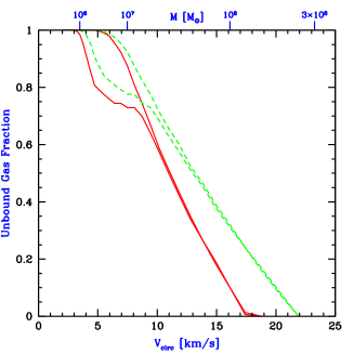
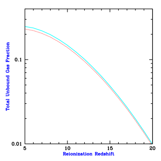
Figure 50: Effect of photo-evaporation on individual halos and on the overall halo population. The left panel shows the unbound gas fraction (within the virial radius) versus total halo velocity dispersion or mass, adopted from Figure 3 of Barkana & Loeb (1999) BL99 . The two pairs of curves correspond to spectral index $\alpha=5$ (solid) or $\alpha=1.8$ (dashed), in each case at $z=8$. In each pair, assuming an optically-thin halo leads to the upper curve, while the lower curve shows the result of including radiative transfer and self shielding. The right panel shows the total fraction of gas in the Universe which evaporates from halos at reionization, versus the reionization redshift, adopted from Figure 7 of Barkana & Loeb (1999) BL99 . The solid line assumes a spectral index $\alpha=1.8$, and the dotted line assumes $\alpha=5$.

Given the values of the unbound gas fraction in halos of different masses, the Press-Schechter mass function (§4.1) can be used to calculate the total fraction of the IGM which goes through the process of accreting onto a halo and then being recycled into the IGM at reionization. The low-mass cutoff in this sum over halos is given by the lowest mass halo in which gas has assembled by the reionization redshift. This mass can be estimated by the linear Jeans mass $M_{\rm J}$ in equation (62). The Jeans mass does not in general precisely equal the limiting mass for accretion (see the discussion in the next section). Indeed, at a given redshift some gas can continue to fall into halos of lower mass than the Jeans mass at that redshift. On the other hand, the larger Jeans mass at higher redshifts means that a time-averaged Jeans mass may be more appropriate, as indicated by the filtering mass. In practice, the Jeans mass is sufficiently accurate since at $z\sim 10$–20 it agrees well with the values found in the numerical spherical collapse calculations of Haiman, Thoul, & Loeb (1996) Haiman .

The right panel of Figure 50 (adopted from Fig. 7 of Barkana & Loeb 1999 BL99 ) shows the total fraction of gas in the Universe which evaporates from halos at reionization, versus the reionization redshift. The solid line assumes a spectral index $\alpha=1.8$, and the dotted line assumes $\alpha=5$, showing that the result is insensitive to the spectrum. Even at high redshift, the amount of gas which participates in photo-evaporation is significant, which suggests a number of possible implications as discussed below. The gas fraction shown in the figure represents most ($\sim 60$–$80\%$ depending on the redshift) of the collapsed fraction before reionization, although some gas does remain in more massive halos.

The photo-evaporation of gas out of large numbers of halos may have interesting implications. First, gas which falls into halos and is expelled at reionization attains a different entropy than if it had stayed in the low-density IGM. The resulting overall reduction in the entropy is expected to be small – the same as would be produced by reducing the temperature of the entire IGM by a factor of $\sim 1.5$ – but localized effects near photo-evaporating halos may be more significant. Furthermore, the resulting $\sim 20~{}{\rm km~{}s^{-1}}$ outflows induce small-scale fluctuations in peculiar velocity and temperature. These outflows are usually well below the resolution limit of most numerical simulations, but some outflows were resolved in the simulation of Bryan et al. (1998) BMAN98 . The evaporating halos may consume a significant number of ionizing photons in the post-overlap stage of reionization HAM00 ; Iliev05 , but a definitive determination requires detailed simulations which include the three-dimensional geometry of source halos and sink halos.

Although gas is quickly expelled out of the smallest halos, photo-evaporation occurs more gradually in larger halos which retain some of their gas. These surviving halos initially expand but they continue to accrete dark matter and to merge with other halos. These evaporating gas halos could contribute to the high column density end of the Ly$\alpha$ forest BSS88 . Abel & Mo (1998) AM98 suggested that, based on the expected number of surviving halos, a large fraction of the Lyman limit systems at $z\sim 3$ may correspond to mini-halos that survived reionization. Surviving halos may even have identifiable remnants in the present Universe. These ideas thus offer the possibility that a population of halos which originally formed prior to reionization may correspond almost directly to several populations that are observed much later in the history of the Universe. However, the detailed dynamics of photo-evaporating halos are complex, and detailed simulations are required to confirm these ideas. Photo-evaporation of a gas cloud has been followed in a two dimensional simulation with radiative transfer, by Shapiro & Raga (2000) SR00 . They found that an evaporating halo would indeed appear in absorption as a damped Ly$\alpha$ system initially, and as a weaker absorption system subsequently. Future simulations Iliev05 will clarify the contribution to quasar absorption lines of the entire population of photo-evaporating halos.

7.5 Suppression of the Formation of Low Mass Galaxies

At the end of overlap, the cosmic ionizing background increased sharply, and the IGM was heated by the ionizing radiation to a temperature $>10^{4}$ K. Due to the substantial increase in the IGM temperature, the intergalactic Jeans mass increased dramatically, changing the minimum mass of forming galaxies MJR86 ; EF92 ; G097 ; MR98 .

Gas infall depends sensitively on the Jeans mass. When a halo more massive than the Jeans mass begins to form, the gravity of its dark matter overcomes the gas pressure. Even in halos below the Jeans mass, although the gas is initially held up by pressure, once the dark matter collapses its increased gravity pulls in some gas Haiman . Thus, the Jeans mass is generally higher than the actual limiting mass for accretion. Before reionization, the IGM is cold and neutral, and the Jeans mass plays a secondary role in limiting galaxy formation compared to cooling. After reionization, the Jeans mass is increased by several orders of magnitude due to the photoionization heating of the IGM, and hence begins to play a dominant role in limiting the formation of stars. Gas infall in a reionized and heated Universe has been investigated in a number of numerical simulations. Thoul & Weinberg (1996) Th96 inferred, based on a spherically-symmetric collapse simulation, a reduction of $\sim 50\%$ in the collapsed gas mass due to heating, for a halo of circular velocity $V_{c}\sim 50\ {\rm km\ s}^{-1}$ at $z=2$, and a complete suppression of infall below $V_{c}\sim 30\ {\rm km\ s}^{-1}$. Kitayama & Ikeuchi (2000) KI00 also performed spherically-symmetric simulations but included self-shielding of the gas, and found that it lowers the circular velocity thresholds by $\sim 5\ {\rm km\ s}^{-1}$. Three dimensional numerical simulations QKE96 ; WHK97 ; NS97 found a significant suppression of gas infall in even larger halos ($V_{c}\sim 75\ {\rm km\ s}^{-1}$), but this was mostly due to a suppression of late infall at $z<2$.

When a volume of the IGM is ionized by stars, the gas is heated to a temperature $T_{\rm IGM}\sim 10^{4}$ K. If quasars dominate the UV background at reionization, their harder photon spectrum leads to $T_{\rm IGM}>2\times 10^{4}$ K. Including the effects of dark matter, a given temperature results in a linear Jeans mass corresponding to a halo circular velocity of

$$V_{J}=81\left(\frac{T_{\rm IGM}}{1.5\times 10^{4}{\rm K}}\right)^{1/2}\ \left[\frac{1}{{\Omega_{m}^{\,z}}}\ \frac{\Delta_{c}}{18\pi^{2}}\right]^{1/6}\ {\rm km\ s}^{-1},$$ (142)

where we used equation (91) and assumed $\mu=0.6$. In halos with $V_{c}>V_{J}$, the gas fraction in infalling gas equals the universal mean of $\Omega_{b}/\Omega_{m}$, but gas infall is suppressed in smaller halos. Even for a small dark matter halo, once it collapses to a virial overdensity of $\Delta_{c}/{\Omega_{m}^{\,z}}$ relative to the mean, it can pull in additional gas. A simple estimate of the limiting circular velocity, below which halos have essentially no gas infall, is obtained by substituting the virial overdensity for the mean density in the definition of the Jeans mass. The resulting estimate is

$$V_{\rm lim}=34\left(\frac{T_{\rm IGM}}{1.5\times 10^{4}{\rm K}}\right)^{1/2}\ {\rm km\ s}^{-1}.$$ (143)

This value is in rough agreement with the numerical simulations mentioned before. A more recent study by Dijkstra et al. (2004) Dijkstra04 indicates that at the high redshifts of $z>10$ gas could nevertheless assemble into halos with circular velocities as low as $v_{c}\sim 10~{}{\rm km~{}s^{-1}}$, even in the presence of a UV background.

Although the Jeans mass is closely related to the rate of gas infall at a given time, it does not directly yield the total gas residing in halos at a given time. The latter quantity depends on the entire history of gas accretion onto halos, as well as on the merger histories of halos, and an accurate description must involve a time-averaged Jeans mass. Gnedin Gnedin2000b showed that the gas content of halos in simulations is well fit by an expression which depends on the filtering mass, a particular time-averaged Jeans mass (Gnedin & Hui 1998 Gnedin98 ). Gnedin Gnedin2000b calculated the Jeans and filtering masses using the mean temperature in the simulation to define the sound speed, and found the following fit to the simulation results:

$$\bar{M_{g}}=\frac{f_{b}M}{\left[1+\left(2^{1/3}-1\right)M_{C}/M\right]^{3}}\ ,$$ (144)

where $\bar{M_{g}}$ is the average gas mass of all objects with a total mass $M$, $f_{b}=\Omega_{b}/{\Omega_{m}}$ is the universal baryon fraction, and the characteristic mass $M_{C}$ is the total mass of objects which on average retain $50\%$ of their gas mass. The characteristic mass was well fit by the filtering mass at a range of redshifts from $z=4$ up to $z\sim 15$.

The reionization process was not perfectly synchronized throughout the Universe. Large-scale regions with a higher density than the mean tend to form galaxies first and reionize earlier than underdense regions (see detailed discussion in §174). The suppression of low-mass galaxies by reionization will therefore be modulated by the fluctuations in the timing of reionization. Babich & Loeb (2005) Bab considered the effect of inhomogeneous reionization on the power-spectrum of low-mass galaxies. They showed that the shape of the high redshift galaxy power spectrum on small scales in a manner which depends on the details of epoch of reionization. This effect is significantly larger than changes in the galaxy power spectrum due to the current uncertainty in the inflationary parameters, such as the tilt of the scalar power spectrum $n$ and the running of the tilt $\alpha$. Therefore, future high redshift galaxies surveys hoping to constrain inflationary parameters must properly model the effects of reionization, but conversely they will also be sensitive to the thermal history of the high redshift intergalactic medium.

8 Feedback from Galactic Outflows

8.1 Propagation of Supernova Outflows in the IGM

Star formation is accompanied by the violent death of massive stars in supernova explosions. In general, if each halo has a fixed baryon fraction and a fixed fraction of the baryons turns into massive stars, then the total energy in supernovae outflows is proportional to the halo mass. The binding energy of the gas in the halo is proportional to the halo mass squared. Thus, outflows are expected to escape more easily out of low-mass galaxies, and to expel a greater fraction of the gas from dwarf galaxies. At high redshifts, most galaxies form in relatively low-mass halos, and the high halo merger rate leads to vigorous star formation. Thus, outflows may have had a great impact on the earliest generations of galaxies, with consequences that may include metal enrichment of the IGM and the disruption of dwarf galaxies. In this subsection we present a simple model for the propagation of individual supernova shock fronts in the IGM. We discuss some implications of this model, but we defer to the following subsection the brunt of the discussion of the cosmological consequences of outflows.

For a galaxy forming in a given halo, the supernova rate is related to the star formation rate. In particular, for a Scalo (1998) Sca98 initial stellar mass function, if we assume that a supernova is produced by each $M>8M_{\odot}$ star, then on average one supernova explodes for every 126 $M_{\odot}$ of star formation, expelling an ejecta mass of $\sim 3\,M_{\odot}$ including $\sim 1\,M_{\odot}$ of heavy elements. We assume that the individual supernovae produce expanding hot bubbles which merge into a single overall region delineated by an outwardly moving shock front. We assume that most of the baryons in the outflow lie in a thin shell, while most of the thermal energy is carried by the hot interior. The total ejected mass equals a fraction $f_{\rm gas}$ of the total halo gas which is lifted out of the halo by the outflow. This gas mass includes a fraction $f_{\rm eject}$ of the mass of the supernova ejecta itself (with $f_{\rm eject}\leq 1$ since some metals may be deposited in the disk and not ejected). Since at high redshift most of the halo gas is likely to have cooled onto a disk, we assume that the mass carried by the outflow remains constant until the shock front reaches the halo virial radius. We assume an average supernova energy of $10^{51}E_{51}$ erg, a fraction $f_{\rm wind}$ of which remains in the outflow after it escapes from the disk. The outflow must overcome the gravitational potential of the halo, which we assume to have a Navarro, Frenk, & White (1997) Na97 density profile [NFW; see equation (94)]. Since the entire shell mass must be lifted out of the halo, we include the total shell mass as well as the total injected energy at the outset. This assumption is consistent with the fact that the burst of star formation in a halo is typically short compared to the total time for which the corresponding outflow expands.

The escape of an outflow from an NFW halo depends on the concentration parameter $c_{\rm N}$ of the halo. Simulations by Bullock et al. (2000) Bu00 indicate that the concentration parameter decreases with redshift, and their results may be extrapolated to our regime of interest (i.e., to smaller halo masses and higher redshifts) by assuming that

$$c_{\rm N}=\left(\frac{M}{10^{9}M_{\odot}}\right)^{-0.1}\,\frac{25}{(1+z)}\ .$$ (145)

Although we calculate below the dynamics of each outflow in detail, it is also useful to estimate which halos can generate large-scale outflows by comparing the kinetic energy of the outflow to the potential energy needed to completely escape (i.e., to infinite distance) from an NFW halo. We thus find that the outflow can escape from its originating halo if the circular velocity is below a critical value given by

$$V_{\rm crit}=200\sqrt{\frac{E_{51}f_{\rm wind}(\eta/0.1)}{f_{\rm gas}\ g(c_{\rm N})}}\ {\rm km\ s}^{-1}\ ,$$ (146)

where the efficiency $\eta$ is the fraction of baryons incorporated in stars, and

$$g(x)=\frac{x^{2}}{(1+x)\ln(1+x)-x}\ .$$ (147)

Note that the contribution to $f_{\rm gas}$ of the supernova ejecta itself is $0.024\eta f_{\rm eject}$, so the ejecta mass is usually negligible unless $f_{\rm gas}<1\%$. Equation (146) can also be used to yield the maximum gas fraction $f_{\rm gas}$ which can be ejected from halos, as a function of their circular velocity. Although this equation is most general, if we assume that the parameters $f_{\rm gas}$ and $f_{\rm wind}$ are independent of $M$ and $z$ then we can normalize them based on low-redshift observations. If we specify $c_{\rm N}\sim 10$ (with $g(10)=6.1$) at $z=0$, then setting $E_{51}=1$ and $\eta=10\%$ yields the required energy efficiency as a function of the ejected halo gas fraction:

$$f_{\rm wind}=1.5f_{\rm gas}\left[\frac{V_{\rm crit}}{100\ {\rm km\ s}^{-1}}\right]^{2}\ .$$ (148)

A value of $V_{\rm crit}\sim 100\ {\rm km\ s}^{-1}$ is suggested by several theoretical and observational arguments which are discussed in the next subsection. However, these arguments are not conclusive, and $V_{\rm crit}$ may differ from this value by a large factor, especially at high redshift (where outflows are observationally unconstrained at present). Note the degeneracy between $f_{\rm gas}$ and $f_{\rm wind}$ which remains even if $V_{\rm crit}$ is specified. Thus, if $V_{\rm crit}\sim 100\ {\rm km\ s}^{-1}$ then a high efficiency $f_{\rm wind}\sim 1$ is required to eject most of the gas from all halos with $V_{c}<V_{\rm crit}$, but only $f_{\rm wind}\sim 10\%$ is required to eject 5–10$\%$ of the gas. The evolution of the outflow does depend on the value of $f_{\rm wind}$ and not just the ratio $f_{\rm wind}/f_{\rm gas}$, since the shell accumulates material from the IGM which eventually dominates over the initial mass carried by the outflow.

We solve numerically for the spherical expansion of a galactic outflow, elaborating on the basic approach of Tegmark, Silk, & Evrard (1993) TSE93 . We assume that most of the mass $m$ carried along by the outflow lies in a thin, dense, relatively cool shell of proper radius $R$. The interior volume, while containing only a fraction $f_{\rm int}\ll 1$ of the mass $m$, carries most of the thermal energy in a hot, isothermal plasma of pressure $p_{\rm int}$ and temperature $T$. We assume a uniform exterior gas, at the mean density of the Universe (at each redshift), which may be neutral or ionized, and may exert a pressure $p_{\rm ext}$ as indicated below. We also assume that the dark matter distribution follows the NFW profile out to the virial radius, and is at the mean density of the Universe outside the halo virial radius. Note that in reality an overdense distribution of gas as well as dark matter may surround each halo due to secondary infall.

The shell radius $R$ in general evolves as follows:

$$m\frac{d^{2}R}{dt^{2}}=4\pi R^{2}\delta p-\left(\frac{dR}{dt}-HR\right)\frac{dm}{dt}-\frac{Gm}{R^{2}}\left(M(R)+\frac{1}{2}m\right)+\frac{8}{3}\pi GRm\rho_{\Lambda}\ ,$$ (149)

where the right-hand-side includes forces due to pressure, sweeping up of additional mass, gravity, and a cosmological constant, respectively. The shell is accelerated by internal pressure and decelerated by external pressure, i.e., $\delta p=p_{\rm int}-p_{\rm ext}$. In the gravitational force, $M(R)$ is the total enclosed mass, not including matter in the shell, and $\frac{1}{2}m$ is the effective contribution of the shell mass in the thin-shell approximation OM88 . The interior pressure is determined by energy conservation, and evolves according to TSE93 :

$$\frac{dp_{\rm int}}{dt}=\frac{L}{2\pi R^{3}}-5\,\frac{p_{\rm int}}{R}\,\frac{dR}{dt}\ ,$$ (150)

where the luminosity $L$ incorporates heating and cooling terms. We include in $L$ the supernova luminosity $L_{\rm sn}$ (during a brief initial period of energy injection), cooling terms $L_{\rm cool}$, ionization $L_{\rm ion}$, and dissipation $L_{\rm diss}$. For simplicity, we assume ionization equilibrium for the interior plasma, and a primordial abundance of hydrogen and helium. We include in $L_{\rm cool}$ all relevant atomic cooling processes in hydrogen and helium, i.e., collisional processes, Bremsstrahlung emission, and Compton cooling off the CMB. Compton scattering is the dominant cooling process for high-redshift outflows. We include in $L_{\rm ion}$ only the power required to ionize the incoming hydrogen upstream, at the energy cost of 13.6 eV per hydrogen atom. The interaction between the expanding shell and the swept-up mass dissipates kinetic energy. The fraction $f_{d}$ of this energy which is re-injected into the interior depends on complex processes occurring near the shock front, including turbulence, non-equilibrium ionization and cooling, and so (following Tegmark et al. 1993 TSE93 ) we let

$$L_{\rm diss}=\frac{1}{2}f_{d}\frac{dm}{dt}\left(\frac{dR}{dt}-HR\right)^{2}\ ,$$ (151)

where we set $f_{d}=1$ and compare below to the other extreme of $f_{d}=0$.

In an expanding Universe, it is preferable to describe the propagation of outflows in terms of comoving coordinates since, e.g., the critical result is the maximum comoving  size of each outflow, since this size yields directly the total IGM mass which is displaced by the outflow and injected with metals. Specifically, we apply the following transformation Shan80 ; Voit96 :

$$d\hat{t}=a^{-2}dt,\ \ \hat{R}=a^{-1}R,\ \ \hat{p}=a^{5}p,\ \hat{\rho}=a^{3}\rho\ .$$ (152)

For ${\Omega_{\Lambda}}=0$, Voit (1996) Voit96 obtained (with the time origin $\hat{t}=0$ at redshift $z_{1}$):

$$\hat{t}=\frac{2}{{\Omega_{m}}H_{0}}\left[\sqrt{1+{\Omega_{m}}z_{1}}-\sqrt{1+{\Omega_{m}}z}\,\right]\ ,$$ (153)

while for ${\Omega_{m}}+{\Omega_{\Lambda}}=1$ there is no simple analytic expression. We set $\beta=\hat{R}/\hat{r}_{\rm vir}$, in terms of the virial radius $r_{\rm vir}$ [equation (90)] of the source halo. We define $\alpha_{S}^{1}$ as the ratio of the shell mass $m$ to $\frac{4}{3}\pi\hat{\rho}_{b}\,\hat{r}_{\rm vir}^{3}$, where $\hat{\rho}_{b}=\rho_{b}(z=0)$ is the mean baryon density of the Universe at $z=0$. More generally, we define

$$\alpha_{S}(\beta)\equiv\frac{m}{\frac{4}{3}\pi\hat{\rho}_{b}\,\hat{\rho}^{3}}=\left\{\begin{array}[]{ll}\alpha_{S}^{1}/\beta^{3}&\mbox{if $\beta<1$}\\ 1+\left(\alpha_{S}^{1}-1\right)/\beta^{3}&\mbox{otherwise.}\end{array}\right.$$ (154)

Here we assumed, as noted above, that the shell mass is constant until the halo virial radius is reached, at which point the outflow begins to sweep up material from the IGM. We thus derive the following equations:

$$\frac{d^{2}\hat{R}}{d\hat{t}^{2}}=\left\{\begin{array}[]{ll}\frac{3}{\alpha_{S}(\beta)}\frac{\hat{p}}{\hat{\rho}_{b}\,\hat{R}}-\frac{a}{2}\hat{R}H_{0}^{2}{\Omega_{m}}\bar{\delta}(\beta)&\mbox{if $\beta<1$}\vspace{.1in}\\ \frac{3}{\alpha_{S}(\beta)\hat{R}}\left[\frac{\hat{p}}{\hat{\rho}_{b}}-\left(\frac{d\hat{R}}{d\hat{t}}\right)^{2}\right]-\frac{a}{2}\hat{R}H_{0}^{2}{\Omega_{m}}\bar{\delta}(\beta)+\frac{a}{4}\hat{R}H_{0}^{2}\Omega_{b}\alpha_{S}(\beta)&\mbox{otherwise,}\end{array}\right.$$ (155)

along with

$$\frac{d}{d\hat{t}}\left(\hat{R}^{5}\hat{p}_{\rm int}\right)=\frac{a^{4}}{2\pi}L\hat{R}^{2}\ .$$ (156)

In the evolution equation for $\hat{R}$, for $\beta<1$ we assume for simplicity that the baryons are distributed in the same way as the dark matter, since in any case the dark matter halo dominates the gravitational force. For $\beta>1$, however, we correct (via the last term on the right-hand side) for the presence of mass in the shell, since at $\beta\gg 1$ this term may become important. The $\beta>1$ equation also includes the braking force due to the swept-up IGM mass. The enclosed mean overdensity for the NFW profile [Eq. (94)] surrounded by matter at the mean density is

$$\bar{\delta}(\beta)=\left\{\begin{array}[]{ll}\frac{\Delta_{c}}{{\Omega_{m}^{\,z}}\beta^{3}}\frac{\ln(1+c_{\rm N}\beta)-c_{\rm N}\beta/(1+c_{\rm N}\beta)}{\ln(1+c)-c/(1+c)}&\mbox{if $\beta<1$}\vspace{.1in}\\ \left(\frac{\Delta_{c}}{{\Omega_{m}^{\,z}}}-1\right)\frac{1}{\beta^{3}}&\mbox{otherwise.}\end{array}\right.$$ (157)

The physics of supernova shells is discussed in Ostriker & McKee (1988) OM88 along with a number of analytical solutions. The propagation of cosmological blast waves has also been computed by Ostriker & Cowie (1981) OC81 , Bertschinger (1985) Be85 and Carr & Ikeuchi (1985) CI85 . Voit (1996) Voit96 derived an exact analytic solution to the fluid equations which, although of limited validity, is nonetheless useful for understanding roughly how the outflow size depends on several of the parameters. The solution requires an idealized case of an outflow which at all times expands into a homogeneous IGM. Peculiar gravitational forces, and the energy lost in escaping from the host halo, are neglected, cooling and ionization losses are also assumed to be negligible, and the external pressure is not included. The dissipated energy is assumed to be retained, i.e., $f_{d}$ is set equal to unity. Under these conditions, the standard Sedov self-similar solution Sed59 ; Sed93 generalizes to the cosmological case as follows Voit96 :

$$\hat{R}=\left(\frac{\xi\hat{E}_{0}}{\hat{\rho}_{b}}\right)^{1/5}\hat{t}^{\,2/5}\ ,$$ (158)

where $\xi=2.026$ and $\hat{E}_{0}=E_{0}/(1+z_{1})^{2}$ in terms of the initial (i.e., at $t=\hat{t}=0$ and $z=z_{1}$) energy $E_{0}$. Numerically, the comoving radius is

$$\hat{R}=280\left(\frac{0.022}{\Omega_{b}h^{2}}\,\frac{E_{0}}{10^{56}{\rm erg}}\right)^{1/5}\left(\frac{10}{1+z_{1}}\,\frac{\hat{t}}{10^{10}{\rm yr}}\right)^{2/5}\ {\rm kpc}\ .$$ (159)

In solving the equations described above, we assume that the shock front expands into a pre-ionized region which then recombines after a time determined by the recombination rate. Thus, the external pressure is included initially, it is turned off after the pre-ionized region recombines, and it is then switched back on at a lower redshift when the Universe is reionized. When the ambient IGM is neutral and the pressure is off, the shock loses energy to ionization. In practice we find that the external pressure is unimportant during the initial expansion, although it is  generally important after reionization. Also, at high redshift ionization losses are much smaller than losses due to Compton cooling. In the results shown below, we assume an instantaneous reionization at $z=9$.

Figure 51 shows the results for a starting redshift $z=15$, for a halo of mass $5.4\times 10^{7}M_{\odot}$, stellar mass $8.0\times 10^{5}M_{\odot}$, comoving $\hat{r}_{\rm vir}=12$ kpc, and circular velocity $V_{c}=20$ km/s. We show the shell comoving radius in units of the virial radius of the source halo (top panel), and the physical peculiar velocity of the shock front (bottom panel). Results are shown (solid curve) for the standard set of parameters $f_{\rm int}=0.1$, $f_{d}=1$, $f_{\rm wind}=75\%$, and $f_{\rm gas}=50\%$. For comparison, we show several cases which adopt the standard parameters except for no cooling (dotted curve), no reionization (short-dashed curve), $f_{d}=0$ (long-dashed curve), or $f_{\rm wind}=15\%$ and $f_{\rm gas}=10\%$ (dot-short dashed curve). When reionization is included, the external pressure halts the expanding bubble. We freeze the radius at the point of maximum expansion (where $d\hat{R}/d\hat{t}=0$), since in reality the shell will at that point begin to spread and fill out the interior volume due to small-scale velocities in the IGM. For the chosen parameters, the bubble easily escapes from the halo, but when $f_{\rm wind}$ and $f_{\rm gas}$ are decreased the accumulated IGM mass slows down the outflow more effectively. In all cases the outflow reaches a size of 10–20 times $\hat{r}_{\rm vir}$, i.e., 100–200 comoving kpc. If all the metals are ejected (i.e., $f_{\rm eject}=1$), then this translates to an average metallicity in the shell of $\sim 1$–5$\times 10^{-3}$ in units of the solar metallicity (which is $2\%$ by mass). The asymptotic size of the outflow varies roughly as $f_{\rm wind}^{1/5}$, as predicted by the simple solution in equation (158), but the asymptotic size is rather insensitive to $f_{\rm gas}$ (at a fixed $f_{\rm wind}$) since the outflow mass becomes dominated by the swept-up IGM mass once $\hat{R}>4\hat{r}_{\rm vir}$. With the standard parameter values (i.e., those corresponding to the solid curve), Figure 51 also shows (dot-long dashed curve) the Voit (1996) Voit96 solution of equation (158). The Voit solution behaves similarly to the no-reionization curve at low redshift, although it overestimates the shock radius by $\sim 30\%$, and the overestimate is greater compared to the more realistic case which does include reionization.

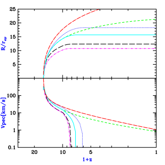
Figure 51: Evolution of a supernova outflow from a $z=15$ halo of circular velocity $V_{c}=20$ km/s. Plotted are the shell comoving radius in units of the virial radius of the source halo (top panel), and the physical peculiar velocity of the shock front (bottom panel). Results are shown for the standard parameters $f_{\rm int}=0.1$, $f_{d}=1$, $f_{\rm wind}=75\%$, and $f_{\rm gas}=50\%$ (solid curve). Also shown for comparison are the cases of no cooling (dotted curve), no reionization (short-dashed curve), $f_{d}=0$ (long-dashed curve), or $f_{\rm wind}=15\%$ and $f_{\rm gas}=10\%$ (dot-short dashed curve), as well as the simple Voit (1996) Voit96 solution of equation (158) for the standard parameter set (dot-long dashed curve). In cases where the outflow halts, we freeze the radius at the point of maximum expansion.

Figure 52 shows different curves than Figure 51 but on an identical layout. A single curve starting at $z=15$ (solid curve) is repeated from Figure 51, and it is compared here to outflows with the same parameters but starting at $z=20$ (dotted curve), $z=10$ (short-dashed curve), and $z=5$ (long-dashed curve). A $V_{c}=20$ km/s halo, with a stellar mass equal to $1.5\%$ of the total halo mass, is chosen at the three higher redshifts, but at $z=5$ a $V_{c}=42$ km/s halo is assumed. Because of the suppression of gas infall after reionization, we assume that the $z=5$ outflow is produced by supernovae from a stellar mass equal to only $0.3\%$ of the total halo mass (with a similarly reduced initial shell mass), thus leading to a relatively small final shell radius. The main conclusion from both figures is the following: In all cases, the outflow undergoes a rapid initial expansion over a fractional redshift interval $\delta z/z\sim 0.2$, at which point the shell has slowed down to $\sim 10$ km/s from an initial 300 km/s. The rapid deceleration is due to the accumulating IGM mass. External pressure from the reionized IGM completely halts all high-redshift outflows, and even without this effect most outflows would only move at $\sim 10$ km/s after the brief initial expansion. Thus, it may be possible for high-redshift outflows to pollute the Lyman alpha forest with metals without affecting the forest hydrodynamically at $z<4$. While the bulk velocities of these outflows may dissipate quickly, the outflows do sweep away the IGM and create empty bubbles. The resulting effects on observations of the Lyman alpha forest should be studied in detail (some observational signatures of feedback have been suggested recently by Theuns, Mo, & Schaye 2000 TMS00 ).

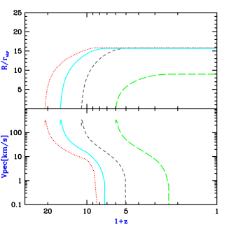
Figure 52: Evolution of supernova outflows at different redshifts. The top and bottom panels are arranged similarly to Figure 51. The $z=15$ outflow (solid curve) is repeated from Figure 51, and it is compared here to outflows with the same parameters but starting at $z=20$ (dotted curve), $z=10$ (short-dashed curve), and $z=5$ (long-dashed curve). A $V_{c}=20$ km/s halo is assumed except for $z=5$, in which case a $V_{c}=42$ km/s halo is assumed to produce the outflow (see text).

Furlanetto & Loeb (2003) FL03 derived the evolution of the characteristic scale and filling fraction of supernova-driven bubbles based on a refinement of this formalism (see also their 2001 paper for quasar-driven outflows). The role of metal-rich outflows in smearing the transition epoch between Pop-III (metal-free) and Pop II (metal-enriched) stars, was also analysed by Furlanetto & Loeb (2005) FL05 , who concluded that a double-reionization history in which the ionization fraction goes through two (or more) peaks is unlikely.

8.2 Effect of Outflows on Dwarf Galaxies and on the IGM

Galactic outflows represent a complex feedback process which affects the evolution of cosmic gas through a variety of phenomena. Outflows inject hydrodynamic energy into the interstellar medium of their host galaxy. As shown in the previous subsection, even a small fraction of this energy suffices to eject most of the gas from a dwarf galaxy, perhaps quenching further star formation after the initial burst. At the same time, the enriched gas in outflows can mix with the interstellar medium and with the surrounding IGM, allowing later generations of stars to form more easily because of metal-enhanced cooling. On the other hand, the expanding shock waves may also strip gas in surrounding galaxies and suppress star formation.

Dekel & Silk (1986) DS86 attempted to explain the different properties of diffuse dwarf galaxies in terms of the effect of galactic outflows. They noted the observed trends whereby lower-mass dwarf galaxies have a lower surface brightness and metallicity, but a higher mass-to-light ratio, than higher mass galaxies. They argued that these trends are most naturally explained by substantial gas removal from an underlying dark matter potential. Galaxies lying in small halos can eject their remaining gas after only a tiny fraction of the gas has turned into stars, while larger galaxies require more substantial star formation before the resulting outflows can expel the rest of the gas. Assuming a wind efficiency $f_{\rm wind}\sim 100\%$, Dekel & Silk showed that outflows in halos below a circular velocity threshold of $V_{\rm crit}\sim 100$ km/s have sufficient energy to expel most of the halo gas. Furthermore, cooling is very efficient for the characteristic gas temperatures associated with $V_{\rm crit}<100$ km/s halos, but it becomes less efficient in more massive halos. As a result, this critical velocity is expected to signify a dividing line between bright galaxies and diffuse dwarf galaxies. Although these simple considerations may explain a number of observed trends, many details are still not conclusively determined. For instance, even in galaxies with sufficient energy to expel the gas, it is possible that this energy gets deposited in only a small fraction of the gas, leaving the rest almost unaffected.

Since supernova explosions in an inhomogeneous interstellar medium lead to complicated hydrodynamics, in principle the best way to determine the basic parameters discussed in the previous subsection ($f_{\rm wind}$, $f_{\rm gas}$, and $f_{\rm eject}$) is through detailed numerical simulations of individual galaxies. Mac Low & Ferrara (1999) Mac99 simulated a gas disk within a $z=0$ dark matter halo. The disk was assumed to be azimuthally symmetric and initially smooth. They represented supernovae by a central source of energy and mass, assuming a constant luminosity which is maintained for 50 million years. They found that the hot, metal-enriched ejecta can in general escape from the halo much more easily than the colder gas within the disk, since the hot gas is ejected in a tube perpendicular to the disk without displacing most of the gas in the disk. In particular, most of the metals were expelled except for the case with the most massive halo considered (with $10^{9}M_{\odot}$ in gas) and the lowest luminosity ($10^{37}$ erg/s, or a total injection of $2\times 10^{52}$ erg). On the other hand, only a small fraction of the total gas mass was ejected except for the least massive halo (with $10^{6}M_{\odot}$ in gas), where a luminosity of $10^{38}$ erg/s or more expelled most of the gas. We note that beyond the standard issues of numerical resolution and convergence, there are several difficulties in applying these results to high-redshift dwarf galaxies. Clumping within the expanding shells or the ambient interstellar medium may strongly affect both the cooling and the hydrodynamics. Also, the effect of distributing the star formation throughout the disk is unclear since in that case several characteristics of the problem will change; many small explosions will distribute the same energy over a larger gas volume than a single large explosion [as in the Sedov (1959) Sed59 solution; see, e.g., equation (158)], and the geometry will be different as each bubble tries to dig its own escape route through the disk. Also, high-redshift disks should be denser by orders of magnitude than $z=0$ disks, due to the higher mean density of the Universe at early times. Thus, further numerical simulations of this process are required in order to assess its significance during the reionization epoch.

Some input on these issues also comes from observations. Martin (1999) Mart99 showed that the hottest extended X-ray emission in galaxies is characterized by a temperature of $\sim 10^{6.7}$ K. This hot gas, which is lifted out of the disk at a rate comparable to the rate at which gas goes into new stars, could escape from galaxies with rotation speeds of $<130$ km/s. However, these results are based on a small sample which includes only the most vigorous star-forming local galaxies, and the mass-loss rate depends on assumptions about the poorly understood transfer of mass and energy among the various phases of the interstellar medium.

Many authors have attempted to estimate the overall cosmological effects of outflows by combining simple models of individual outflows with the formation rate of galaxies, obtained via semi-analytic methods CR86 ; TSE93 ; Voit96 ; NT97 ; FPS00 ; SB00 or numerical simulations G097 ; Gne98 ; CO99 ; AHWKG2000a . The main goal of these calculations is to explain the characteristic metallicities of different environments as a function of redshift. For example, the IGM is observed to be enriched with metals at redshifts $z<5$. Identification of C IV, Si IV an O VI absorption lines which correspond to Ly$\alpha$ absorption lines in the spectra of high-redshift quasars has revealed that the low-density IGM has been enriched to a metal abundance (by mass) of $Z_{\rm IGM}\sim 10^{-2.5(\pm 0.5)}Z_{\odot}$, where $Z_{\odot}=0.019$ is the solar metallicity MY87 ; Tyt95 ; SC96 ; LSBR98 ; CS98 ; Song97 ; ESSP00 . The metal enrichment has been clearly identified down to H I column densities of $\sim 10^{14.5}~{}{\rm cm^{-2}}$. The detailed comparison of cosmological hydrodynamic simulations with quasar absorption spectra has established that the forest of Ly$\alpha$ absorption lines is caused by the smoothly-fluctuating density of the neutral component of the IGM CMOR94 ; ZAN95 ; HKWM96 . The simulations show a strong correlation between the H I column density and the gas overdensity $\delta_{\rm gas}$ DHKW99 , implying that metals were dispersed into regions with an overdensity as low as $\delta_{\rm gas}\sim 3$ or possibly even lower.

In general, dwarf galaxies are expected to dominate metal enrichment at high-redshift for several reasons. As noted above and in the previous subsection, outflows can escape more easily out of the potential wells of dwarfs. Also, at high redshift, massive halos are rare and dwarf halos are much more common. Finally, as already noted, the Sedov (1959) Sed59 solution [or equation (158)] implies that for a given total energy and expansion time, multiple small outflows fill large volumes more effectively than would a smaller number of large outflows. Note, however, that the strong effect of feedback in dwarf galaxies may also quench star formation rapidly and reduce the efficiency of star formation in dwarfs below that found in more massive galaxies.

Cen & Ostriker (1999) CO99 showed via numerical simulation that metals produced by supernovae do not mix uniformly over cosmological volumes. Instead, at each epoch the highest density regions have much higher metallicity than the low-density IGM. They noted that early star formation occurs in the most overdense regions, which therefore reach a high metallicity (of order a tenth of the solar value) by $z\sim 3$, when the IGM metallicity is lower by 1–2 orders of magnitude. At later times, the formation of high-temperature clusters in the highest-density regions suppresses star formation there, while lower-density regions continue to increase their metallicity. Note, however, that the spatial resolution of the hydrodynamic code of Cen & Ostriker is a few hundred kpc, and anything occurring on smaller scales is inserted directly via simple parametrized models. Scannapieco & Broadhurst (2000) SB00 implemented expanding outflows within a numerical scheme which, while not a full gravitational simulation, did include spatial correlations among halos. They showed that winds from low-mass galaxies may also strip gas from nearby galaxies (see also Scannapieco, Ferrara, & Broadhurst 2000 SFB00 ), thus suppressing star formation in a local neighborhood and substantially reducing the overall abundance of galaxies in halos below a mass of $\sim 10^{10}M_{\odot}$. Although quasars do not produce metals, they may also affect galaxy formation in their vicinity via energetic outflows ER88 ; BW91 ; Sil98 ; NSS98 .

Gnedin & Ostriker (1997) G097 and Gnedin (1998) Gne98 identified another mixing mechanism which, they argued, may be dominant at high redshift ($z>4$). In a collision between two protogalaxies, the gas components collide in a shock and the resulting pressure force can eject a few percent of the gas out of the merger remnant. This is the merger mechanism, which is based on gravity and hydrodynamics rather than direct stellar feedback. Even if supernovae inject most of their metals in a local region, larger-scale mixing can occur via mergers. Note, however, that Gnedin’s (1998) Gne98 simulation assumed a comoving star formation rate at $z>5$ of $\sim 1M_{\odot}$ per year per comoving Mpc³, which is 5–10 times larger than the observed rate at redshift 3–4. Aguirre et al. AHWKG2000a used outflows implemented in simulations to conclude that winds of $\sim 300$ km/s at $z<6$ can produce the mean metallicity observed at $z\sim 3$ in the Ly$\alpha$ forest. In a separate paper Aguirre et al. AHKGW2000b explored another process, where metals in the form of dust grains are driven to large distances by radiation pressure, thus producing large-scale mixing without displacing or heating large volumes of IGM gas. The success of this mechanism depends on detailed microphysics such as dust grain destruction and the effect of magnetic fields. The scenario, though, may be directly testable because it leads to significant ejection only of elements which solidify as grains.

Feedback from galactic outflows encompasses a large variety of processes and influences. The large range of scales involved, from stars or quasars embedded in the interstellar medium up to the enriched IGM on cosmological scales, make possible a multitude of different, complementary approaches, promising to keep galactic feedback an active field of research.

9 The Frontier of 21cm Cosmology

9.1 Mapping Hydrogen Before Reionization

The small residual fraction of free electrons after cosmological recombination coupled the temperature of the cosmic gas to that of the cosmic microwave background (CMB) down to a redshift, $z\sim 200$ Peebles . Subsequently, the gas temperature dropped adiabatically as $T_{\rm gas}\propto(1+z)^{2}$ below the CMB temperature $T_{\gamma}\propto(1+z)$. The gas heated up again after being exposed to the photo-ionizing ultraviolet light emitted by the first stars during the reionization epoch at $z<20$. Prior to the formation of the first stars, the cosmic neutral hydrogen must have resonantly absorbed the CMB flux through its spin-flip 21cm transition Field ; Scott ; Tozzi ; Zalda04 . The linear density fluctuations at that time should have imprinted anisotropies on the CMB sky at an observed wavelength of $\lambda=21.12[(1+z)/100]$ meters. We discuss these early 21cm fluctuations mainly for pedagogical purposes. Detection of the earliest 21cm signal will be particularly challenging because the foreground sky brightness rises as $\lambda^{2.5}$ at long wavelengths in addition to the standard $\sqrt{\lambda}$ scaling of the detector noise temperature for a given integration time and fractional bandwidth. The discussion in this section follows Loeb & Zaldarriaga (2004) Loeb04 .

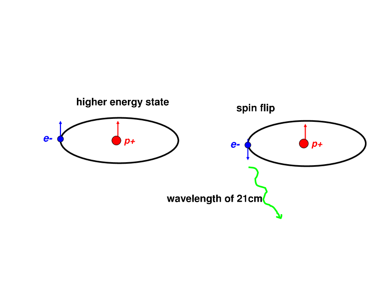
Figure 53: The 21cm transition of hydrogen. The higher energy level the spin of the electron (e-) is aligned with that of the proton (p+). A spin flip results in the emission of a photon with a wavelength of 21cm (or a frequency of 1420MHz).

We start by calculating the history of the spin temperature, $T_{s}$, defined through the ratio between the number densities of hydrogen atoms in the excited and ground state levels, ${n_{1}/n_{0}}=(g_{1}/g_{0})\exp\left\{-{T_{\star}/T_{s}}\right\},$

$${n_{1}\over n_{0}}={g_{1}\over g_{0}}\exp\left\{-{T_{\star}\over T_{s}}\right\},$$ (160)

where subscripts $1$ and $0$ correspond to the excited and ground state levels of the 21cm transition, $(g_{1}/g_{0})=3$ is the ratio of the spin degeneracy factors of the levels, $n_{\rm H}=(n_{0}+n_{1})\propto(1+z)^{3}$ is the total hydrogen density, and $T_{\star}=0.068$K is the temperature corresponding to the energy difference between the levels. The time evolution of the density of atoms in the ground state is given by,

$$\left({\partial\over\partial t}+3{{\dot{a}}\over a}\right) n_{0} =-n_{0}\left(C_{01}+B_{01}I_{\nu}\right)$$

$$+ n_{1} \left(C_{10}+A_{10}+B_{10}I_{\nu}\right),$$ (161)

where $a(t)=(1+z)^{-1}$ is the cosmic scale factor, $A$’s and $B$’s are the Einstein rate coefficients, $C$’s are the collisional rate coefficients, and $I_{\nu}$ is the blackbody intensity in the Rayleigh-Jeans tail of the CMB, namely $I_{\nu}=2kT_{\gamma}/\lambda^{2}$ with $\lambda=21$ cm RL . Here a dot denotes a time-derivative. The $0\rightarrow 1$ transition rates can be related to the $1\rightarrow 0$ transition rates by the requirement that in thermal equilibrium with $T_{s}=T_{\gamma}=T_{\rm gas}$, the right-hand-side of Eq. (161) should vanish with the collisional terms balancing each other separately from the radiative terms. The Einstein coefficients are $A_{10}=2.85\times 10^{-15}~{}{\rm s^{-1}}$, $B_{10}=(\lambda^{3}/2hc)A_{10}$ and $B_{01}=(g_{1}/g_{0})B_{10}$ Field ; RL . The collisional de-excitation rates can be written as $C_{10}={4\over 3}\kappa(1-0)n_{\rm H}$, where $\kappa(1-0)$ is tabulated as a function of $T_{\rm gas}$ AD ; Zyg .

Equation (161) can be simplified to the form,

$${d\Upsilon\over dz} = -\left[H(1+z)\right]^{-1}\left[-\Upsilon(C_{01}+B_{01}I_{\nu})\right.$$ (162)

$$\left.+(1-\Upsilon)(C_{10}+A_{10}+B_{10}I_{\nu})\right],$$

where $\Upsilon\equiv n_{0}/n_{\rm H}$, $H\approx H_{0}\sqrt{\Omega_{m}}(1+z)^{3/2}$ is the Hubble parameter at high redshifts (with a present-day value of $H_{0}$), and $\Omega_{m}$ is the density parameter of matter. The upper panel of Fig. 54 shows the results of integrating Eq. (162). Both the spin temperature and the kinetic temperature of the gas track the CMB temperature down to $z\sim 200$. Collisions are efficient at coupling $T_{s}$ and $T_{gas}$ down to $z\sim 70$ and so the spin temperature follows the kinetic temperature around that redshift. At much lower redshifts, the Hubble expansion makes the collision rate subdominant relative the radiative coupling rate to the CMB, and so $T_{s}$ tracks $T_{\gamma}$ again. Consequently, there is a redshift window between $30<z<200$, during which the cosmic hydrogen absorbs the CMB flux at its resonant 21cm transition. Coincidentally, this redshift interval precedes the appearance of collapsed objects BL01 and so its signatures are not contaminated by nonlinear density structures or by radiative or hydrodynamic feedback effects from stars and quasars, as is the case at lower redshifts Zalda04 .

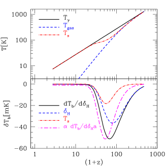
Figure 54: Upper panel: Evolution of the gas, CMB and spin temperatures with redshift [4]. Lower panel: ${dT_{b}/d{\delta_{H}}}$ as function of redshift. The separate contributions from fluctuations in the density and the spin temperature are depicted. We also show ${dT_{b}/d{\delta_{H}}}a\propto{dT_{b}/d{\delta_{H}}}\times{\delta_{H}}$, with an arbitrary normalization.

During the period when the spin temperature is smaller than the CMB temperature, neutral hydrogen atoms absorb CMB photons. The resonant 21cm absorption reduces the brightness temperature of the CMB by,

$$T_{b}=\tau\left(T_{s}-T_{\gamma}\right)/(1+z),$$ (163)

where the optical depth for resonant 21cm absorption is,

$$\tau={3c\lambda^{2}hA_{10}n_{\rm H}\over 32\pi kT_{s}H(z)}.$$ (164)

Small inhomogeneities in the hydrogen density ${\delta_{H}}\equiv(n_{\rm H}-{\bar{n}_{\rm H}})/{\bar{n}}_{\rm H}$ result in fluctuations of the 21cm absorption through two separate effects. An excess of neutral hydrogen directly increases the optical depth and also alters the evolution of the spin temperature. For now, we ignore the additional effects of peculiar velocities (Bharadwaj & Ali 2004 Indian ; Barkana & Loeb 2004 BL04a ) as well as fluctuations in the gas kinetic temperature due to the adiabatic compression (rarefaction) in overdense (underdense) regions BLinf . Under these approximations, we can write an equation for the resulting evolution of $\Upsilon$ fluctuations,

$${d\delta\Upsilon\over dz} = \left[H(1+z)\right]^{-1}\left\{[C_{10}+C_{01}+(B_{01}+B_{10})I_{\nu}]\delta\Upsilon\right.$$ (165)

$$\left.+\left[C_{01}\Upsilon-C_{10}(1-\Upsilon)\right]{\delta_{H}}\right\},$$

leading to spin temperature fluctuations,

$${\delta T_{s}\over{\bar{T}}_{s}}=-{1\over\ln[3\Upsilon/(1-\Upsilon)]}{\delta\Upsilon\over\Upsilon(1-\Upsilon)}.$$ (166)

The resulting brightness temperature fluctuations can be related to the derivative,

$${\delta T_{b}\over{\bar{T}}_{b}}={\delta_{H}}+{T_{\gamma}\over({\bar{T}}_{s}-T_{\gamma})}{\delta T_{s}\over{\bar{T}}_{s}}.$$ (167)

The spin temperature fluctuations ${\delta T_{s}/{T}_{s}}$ are proportional to the density fluctuations and so we define,

$${dT_{b}\over d{\delta_{H}}}\equiv{\bar{T}}_{b}+{T_{\gamma}{\bar{T}}_{b}\over({\bar{T}}_{s}-T_{\gamma})}{\delta T_{s}\over{\bar{T}}_{s}{\delta_{H}}},$$ (168)

through ${\delta T_{b}}=({dT_{b}/d{\delta_{H}}}){\delta_{H}}$. We ignore fluctuations in $C_{ij}$ due to fluctuations in $T_{\rm gas}$ which are very small AD . Figure 54 shows ${dT_{b}/d{\delta_{H}}}$ as a function of redshift, including the two contributions to ${dT_{b}/d{\delta_{H}}}$, one originating directly from density fluctuations and the second from the associated changes in the spin temperature Scott . Both contributions have the same sign, because an increase in density raises the collision rate and lowers the spin temperature and so it allows $T_{s}$ to better track $T_{\rm gas}$. Since ${\delta_{H}}$ grows with time as ${\delta_{H}}\propto a$, the signal peaks at $z\sim 50$, a slightly lower redshift than the peak of ${dT_{b}/d{\delta_{H}}}$.

Next we calculate the angular power spectrum of the brightness temperature on the sky, resulting from density perturbations with a power spectrum $P_{\delta}(k)$,

$$\langle{\delta_{H}}({\bf k}_{1}){\delta_{H}}({\bf k}_{2})\rangle=(2\pi)^{3}\delta^{D}({\bf k}_{1}+{\bf k}_{2})P_{\delta}(k_{1}).$$ (169)

where ${\delta_{H}}({\bf k})$ is the Fourier tansform of the hydrogen density field, ${\bf k}$ is the comoving wavevector, and $\langle\cdots\rangle$ denotes an ensemble average (following the formalism described in Zalda04 ). The 21cm brightness temperature observed at a frequency $\nu$ corresponding to a distance $r$ along the line of sight, is given by

$$\delta T_{b}({\bf n},\nu)=\int drW_{\nu}(r)\ {dT_{b}\over d{\delta_{H}}}{\delta_{H}}({\bf n},r),$$ (170)

where ${\bf n}$ denotes the direction of observation, $W_{\nu}(r)$ is a narrow function of $r$ that peaks at the distance corresponding to $\nu$. The details of this function depend on the characteristics of the experiment. The brightness fluctuations in Eq. 170 can be expanded in spherical harmonics with expansion coefficients $a_{lm}(\nu)$. The angular power spectrum of map $C_{l}(\nu)=\langle|a_{lm}(\nu)|^{2}\rangle$ can be expressed in terms of the 3D power spectrum of fluctuations in the density $P_{\delta}(k)$,

$$C_{l}(\nu) = 4\pi\int{d^{3}k\over(2\pi)^{3}}P_{\delta}(k)\alpha_{l}^{2}(k,\nu)$$

$$\alpha_{l}(k,\nu) = \int drW_{r_{0}}(r){dT_{b}\over d{\delta_{H}}}(r)j_{l}(kr).$$ (171)

Our calculation ignores inhomogeneities in the hydrogen ionization fraction, since they freeze at the earlier recombination epoch ($z\sim 10^{3}$) and so their amplitude is more than an order of magnitude smaller than ${\delta_{H}}$ at $z<100$. The gravitational potential perturbations induce a redshift distortion effect that is of order $\sim(H/ck)^{2}$ smaller than ${\delta_{H}}$ for the high–$l$ modes of interest here.

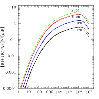
Figure 55: Angular power spectrum of 21cm anisotropies on the sky at various redshifts. From top to bottom, $z=55,40,80,30,120,25,170$.

Figure 55 shows the angular power spectrum at various redshifts. The signal peaks around $z\sim 50$ but maintains a substantial amplitude over the full range of $30<z<100$. The ability to probe the small scale power of density fluctuations is only limited by the Jeans scale, below which the dark matter inhomogeneities are washed out by the finite pressure of the gas. Interestingly, the cosmological Jeans mass reaches its minimum value, $\sim 3\times 10^{4}M_{\odot}$, within the redshift interval of interest here which corresponds to modes of angular scale $\sim$ arcsecond on the sky. During the epoch of reionization, photoionization heating raises the Jeans mass by several orders of magnitude and broadens spectral features, thus limiting the ability of other probes of the intergalactic medium, such as the Ly$\alpha$ forest, from accessing the same very low mass scales. The 21cm tomography has the additional advantage of probing the majority of the cosmic gas, instead of the trace amount ($\sim 10^{-5}$) of neutral hydrogen probed by the Ly$\alpha$ forest after reionization. Similarly to the primary CMB anisotropies, the 21cm signal is simply shaped by gravity, adiabatic cosmic expansion, and well-known atomic physics, and is not contaminated by complex astrophysical processes that affect the intergalactic medium at $z<30$.

Characterizing the initial fluctuations is one of the primary goals of observational cosmology, as it offers a window into the physics of the very early Universe, namely the epoch of inflation during which the fluctuations are believed to have been produced. In most models of inflation, the evolution of the Hubble parameter during inflation leads to departures from a scale-invariant spectrum that are of order $1/N_{\rm efold}$ with $N_{\rm efold}\sim 60$ being the number of $e$–folds between the time when the scale of our horizon was of order the horizon during inflation and the end of inflation lidlith . Hints that the standard $\Lambda$CDM model may have too much power on galactic scales have inspired several proposals for suppressing the power on small scales. Examples include the possibility that the dark matter is warm and it decoupled while being relativistic so that its free streaming erased small-scale power Ba01 , or direct modifications of inflation that produce a cut-off in the power on small scales kamlidd . An unavoidable collisionless component of the cosmic mass budget beyond CDM, is provided by massive neutrinos (see neut for a review). Particle physics experiments established the mass splittings among different species which translate into a lower limit on the fraction of the dark matter accounted for by neutrinos of $f_{\nu}>0.3\%$, while current constraints based on galaxies as tracers of the small scale power imply $f_{\nu}<12\%$ tegsdss .

Figure 56 shows the 21cm power spectrum for various models that differ in their level of small scale power. It is clear that a precise measurement of the 21cm power spectrum will dramatically improve current constraints on alternatives to the standard $\Lambda$CDM spectrum.

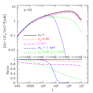
Figure 56: Upper panel: Power spectrum of 21cm anisotropies at $z=55$ for a $\Lambda$CDM scale-invariant power spectrum, a model with $n=0.98$, a model with $n=0.98$ and $\alpha_{r}\equiv{1\over 2}(d^{2}\ln P/d\ln k^{2})=-0.07$, a model of warm dark matter particles with a mass of 1 keV, and a model in which $f_{\nu}=10\%$ of the matter density is in three species of massive neutrinos with a mass of $0.4~{}{\rm eV}$ each. Lower panel: Ratios between the different power spectra and the scale-invariant spectrum.

The 21cm signal contains a wealth of information about the initial fluctuations. A full sky map at a single photon frequency measured up to $l_{\rm max}$, can probe the power spectrum up to $k_{\rm max}\sim(l_{\rm max}/10^{4}){\rm Mpc}^{-1}$. Such a map contains $l_{\rm max}^{2}$ independent samples. By shifting the photon frequency, one may obtain many independent measurements of the power. When measuring a mode $l$, which corresponds to a wavenumber $k\sim l/r$, two maps at different photon frequencies will be independent if they are separated in radial distance by $1/k$. Thus, an experiment that covers a spatial range $\Delta r$ can probe a total of $k\Delta r\sim l\Delta r/r$ independent maps. An experiment that detects the 21cm signal over a range $\Delta\nu$ centered on a frequency $\nu$, is sensitive to $\Delta r/r\sim 0.5(\Delta\nu/\nu)(1+z)^{-1/2}$, and so it measures a total of $N_{\rm 21cm}\sim 3\times 10^{16}(l_{\rm max}/10^{6})^{3}(\Delta\nu/\nu)(z/100)^{-1/2}$ independent samples.

This detection capability cannot be reproduced even remotely by other techniques. For example, the primary CMB anisotropies are damped on small scales (through the so-called Silk damping), and probe only modes with $l\leq 3000$ ($k\leq 0.2\ {\rm Mpc}^{-1}$). The total number of modes available in the full sky is $N_{\rm cmb}=2l_{\rm max}^{2}\sim 2\times 10^{7}(l_{\rm max}/3000)^{2}$, including both temperature and polarization information.

The sensitivity of an experiment depends strongly on its particular design, involving the number and distribution of the antennae for an interferometer. Crudely speaking, the uncertainty in the measurement of $[{l(l+1)C_{l}/2\pi}]^{1/2}$ is dominated by noise, $N_{\nu}$, which is controlled by the sky brightness $I_{\nu}$ at the observed frequency $\nu$ Zalda04 ,

$$N_{\nu} \sim 0.4{\rm mK}\left({I_{\nu}[50{\rm MHz}]\over 5\times 10^{5}{\rm Jy\ sr^{-1}}}\right)\left({l_{\rm min}\over 35}\right)\left({5000\over l_{\rm max}}\right)\left({0.016\over f_{\rm cover}}\right)$$ (172)

$$\times\left({1\ {\rm year}\over t_{0}}\right)^{1/2}\left({\Delta\nu\over 50{\rm MHz}}\right)^{-1/2}\ \left({50\ {\rm MHz}\over\nu}\right)^{2.5},$$

where $l_{\rm min}$ is the minimum observable $l$ as determined by the field of view of the instruments, $l_{\rm max}$ is the maximum observable $l$ as determined by the maximum separation of the antennae, $f_{\rm cover}$ is the fraction of the array area thats is covered by telescopes, $t_{0}$ is the observation time and $\Delta\nu$ is the frequency range over which the signal can be detected. Note that the assumed sky temperature of $0.7\times 10^{4}$K at $\nu=50$MHz (corresponding to $z\sim 30$) is more than six orders of magnitude larger than the signal. We have already included the fact that several independent maps can be produced by varying the observed frequency. The numbers adopted above are appropriate for the inner core of the LOFAR array (http://www.lofar.org), planned for initial operation in 2006. The predicted signal is $\sim 1{\rm mK}$, and so a year of integration or an increase in the covering fraction are required to observe it with LOFAR. Other experiments whose goal is to detect 21cm fluctuations from the subsequent epoch of reionization at $z\sim 6-12$ (when ionized bubbles exist and the fluctuations are larger) include the Mileura Wide-Field Array (MWA; http://web.haystack.mit.edu/arrays/MWA/), the Primeval Structure Telescope (PAST; http://arxiv.org/abs/astro-ph/0502029), and in the more distant future the Square Kilometer Array (SKA; http://www.skatelescope.org). The main challenge in detecting the predicted signal from higher redshifts involves its appearance at low frequencies where the sky noise is high. Proposed space-based instruments RadioAstr avoid the terrestrial radio noise and the increasing atmospheric opacity at $\nu<20\ {\rm MHz}$ (corresponding to $z>70$).

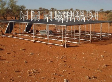
Figure 57: Prototype of the tile design for the Mileura Wide-Field Array (MWA) in western Australia, aimed at detecting redshifted 21cm from the epoch of reionization. Each 4m$\times$4m tile contains 16 dipole antennas operating in the frequency range of 80–300MHz. Altogether the initial phase of MWA (the so-called “Low-Frequency Demostrator”) will include 500 antenna tiles with a total collecting area of 8000 m² at 150MHz, scattered across a 1.5 km region and providing an angular resolution of a few arcminutes.

The 21cm absorption is replaced by 21cm emission from neutral hydrogen as soon as the intergalactic medium is heated above the CMB temperature by X-ray sources during the epoch of reionization ChenMi . This occurs long before reionization since the required heating requires only a modest amount of energy, $\sim 10^{-2}~{}{\rm eV}[(1+z)/30]$, which is three orders of magnitude smaller than the amount necessary to ionize the Universe. As demonstrated by Chen & Miralda-Escude (2004) ChenMi , heating due the recoil of atoms as they absorb Ly$\alpha$ photons Madau is not effective; the Ly$\alpha$ color temperature reaches equilibrium with the gas kinetic temperature and suppresses subsequent heating before the level of heating becomes substantial. Once most of the cosmic hydrogen is reionized at $z_{\rm reion}$, the 21cm signal is diminished. The optical depth for free-free absorption after reionization, $\sim 0.1[(1+z_{\rm reion})/20]^{5/2}$, modifies only slightly the expected 21cm anisotropies. Gravitational lensing should modify the power spectrum Pen at high $l$, but can be separated as in standard CMB studies (see lensing and references therein). The 21cm signal should be simpler to clean as it includes the same lensing foreground in independent maps obtained at different frequencies.

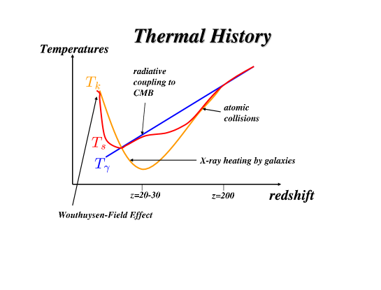
Figure 58: Schematic sketch of the evolution of the kinetic temperature ($T_{k}$) and spin temperature ($T_{s}$) of cosmic hydrogen. Following cosmological recombination at $z\sim 10^{3}$, the gas temperature (orange curve) tracks the CMB temperature (blue line; $T_{\gamma}\propto(1+z)$) down to $z\sim 200$ and then declines below it ($T_{k}\propto(1+z)^{2}$) until the first X-ray sources (accreting black holes or exploding supernovae) heat it up well above the CMB temperature. The spin temperature of the 21cm transition (red curve) interpolates between the gas and CMB temperatures. Initially it tracks the gas temperature through collisional coupling; then it tracks the CMB through radiative coupling; and eventually it tracks the gas temperature once again after the production of a cosmic background of UV photons between the Ly$\alpha$ and the Lyman-limit frequencies that redshift or cascade into the Ly$\alpha$ resonance (through the Wouthuysen-Field effect [Wouthuysen 1952 Wout ; Field 1959 Field ]). Parts of the curve are exaggerated for pedagogic purposes. The exact shape depends on astrophysical details about the first galaxies, such as their production of X-ray binaries, supernovae, nuclear accreting black holes, and their generation of relativistic electrons in collisionless shocks which produce UV and X-ray photons through inverse-Compton scattering of CMB photons.

The large number of independent modes probed by the 21cm signal would provide a measure of non-Gaussian deviations to a level of $\sim N_{\rm 21cm}^{-1/2}$, constituting a test of the inflationary origin of the primordial inhomogeneities which are expected to possess deviations $>10^{-6}$ malda .

9.2 The Characteristic Observed Size of Ionized Bubbles at the End of Reionization

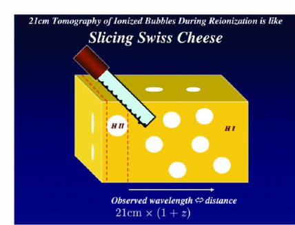
Figure 59: 21cm imaging of ionized bubbles during the epoch of reionization is analogous to slicing swiss cheese. The technique of slicing at intervals separated by the typical dimension of a bubble is optimal for revealing different pattens in each slice.

The first galaxies to appear in the Universe at redshifts $z>20$ created ionized bubbles in the intergalactic medium (IGM) of neutral hydrogen (H I ) left over from the Big-Bang. It is thought that the ionized bubbles grew with time, surrounded clusters of dwarf galaxiesBL04 ; FZH and eventually overlapped quickly throughout the Universe over a narrow redshift interval near $z\sim 6$. This event signaled the end of the reionization epoch when the Universe was a billion years old. Measuring the unknown size distribution of the bubbles at their final overlap phase is a focus of forthcoming observational programs aimed at highly redshifted 21cm emission from atomic hydrogen. In this sub-section we follow Wyithe & Loeb (2004) Bubble and show that the combined constraints of cosmic variance and causality imply an observed bubble size at the end of the overlap epoch of $\sim 10$ physical Mpc, and a scatter in the observed redshift of overlap along different lines-of-sight of $\sim 0.15$. This scatter is consistent with observational constraints from recent spectroscopic data on the farthest known quasars. This result implies that future radio experiments should be tuned to a characteristic angular scale of $\sim 0.5^{\circ}$ and have a minimum frequency band-width of $\sim 8$ MHz for an optimal detection of 21cm flux fluctuations near the end of reionization.

During the reionization epoch, the characteristic bubble size (defined here as the spherically averaged mean radius of the H II regions that contain most of the ionized volumeFZH ) increased with time as smaller bubbles combined until their overlap completed and the diffuse IGM was reionized. However the largest size of isolated bubbles (fully surrounded by H I boundaries) that can be observed is finite, because of the combined phenomena of cosmic variance and causality. Figure 61 presents a schematic illustration of the geometry. There is a surface on the sky corresponding to the time along different lines-of-sight when the diffuse (uncollapsed) IGM was most recently neutral. We refer to it as the Surface of Bubble Overlap (SBO). There are two competing sources for fluctuations in the SBO, each of which is dependent on the characteristic size, $R_{\rm SBO}$, of the ionized regions just before the final overlap. First, the finite speed of light implies that 21cm photons observed from different points along the curved boundary of an H II region must have been emitted at different times during the history of the Universe. Second, bubbles on a comoving scale $R$ achieve reionization over a spread of redshifts due to cosmic variance in the initial conditions of the density field smoothed on that scale. The characteristic scale of H II bubbles grows with time, leading to a decline in the spread of their formation redshiftsBL04 as the cosmic variance is averaged over an increasing spatial volume. However the 21cm light-travel time across a bubble rises concurrently. Suppose a signal 21cm photon which encodes the presence of neutral gas, is emitted from the far edge of the ionizing bubble. If the adjacent region along the line-of-sight has not become ionized by the time this photon reaches the near side of the bubble, then the photon will encounter diffuse neutral gas. Other photons emitted at this lower redshift will therefore also encode the presence of diffuse neutral gas, implying that the first photon was emitted prior to overlap, and not from the SBO. Hence the largest observable scale of H II regions when their overlap completes, corresponds to the first epoch at which the light crossing time becomes larger than the spread in formation times of ionized regions. Only then will the signal photon leaving the far side of the HII region have the lowest redshift of any signal photon along that line-of-sight.

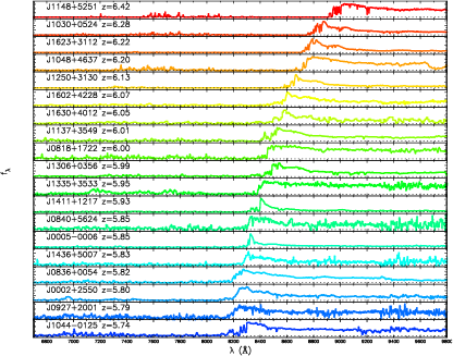
Figure 60: Spectra of 19 quasars with redshifts $5.74<z<6.42$ from the Sloan Digital Sky Survey Fan05 . For some of the highest-redshift quasars, the spectrum shows no transmitted flux shortward of the Ly$\alpha$ wavelength at the quasar redshift (the so-called “Gunn-Peterson trough”), indicating a non-negligible neutral fraction in the IGM (see the analysis of Fan et al. Fan05 for details).

The observed spectra of some quasars beyond $z\sim 6.1$ show a Gunn-Peterson troughGP ; f2 (Fan et al. 2005 Fan05 ), a blank spectral region at wavelengths shorter than Ly$\alpha$ at the quasar redshift, implying the presence of H I in the diffuse IGM. The detection of Gunn-Peterson troughs indicates a rapid changef1 ; Pe ; WB1 in the neutral content of the IGM at $z\sim 6$, and hence a rapid change in the intensity of the background ionizing flux. This rapid change implies that overlap, and hence the reionization epoch, concluded near $z\sim 6$. The most promising observational probeZalda04 ; Miguel1 of the reionization epoch is redshifted 21cm emission from intergalactic H I . Future observations using low frequency radio arrays (e.g. LOFAR, MWA, and PAST) will allow a direct determination of the topology and duration of the phase of bubble overlap. In this section we determine the expected angular scale and redshift width of the 21cm fluctuations at the SBO theoretically, and show that this determination is consistent with current observational constraints.

We start by quantifying the constraints of causality and cosmic variance. First suppose we have an H II region with a physical radius $R/(1+\langle z\rangle)$. For a 21cm photon, the light crossing time of this radius is

$$\langle\Delta z^{2}\rangle^{1/2}=\left|\frac{dz}{dt}\right|_{\langle z\rangle}\frac{R}{c(1+\langle z\rangle)},$$ (173)

where at the high-redshifts of interest $(dz/dt)=-(H_{0}\sqrt{\Omega_{m}})(1+z)^{5/2}$. Here, $c$ is the speed of light, $H_{0}$ is the present-day Hubble constant, $\Omega_{m}$ is the present day matter density parameter, and $\langle z\rangle$ is the mean redshift of the SBO. Note that when discussing this crossing time, we are referring to photons used to probe the ionized bubble (e.g. at 21cm), rather than photons involved in the dynamics of the bubble evolution.

Second, overlap would have occurred at different times in different regions of the IGM due to the cosmic scatter in the process of structure formation within finite spatial volumesBL04 . Reionization should be completed within a region of comoving radius $R$ when the fraction of mass incorporated into collapsed objects in this region attains a certain critical value, corresponding to a threshold number of ionizing photons emitted per baryon. The ionization state of a region is governed by the enclosed ionizing luminosity, by its over-density, and by dense pockets of neutral gas that are self shielding to ionizing radiation. There is an offset BL04 $\delta z$ between the redshift when a region of mean over-density $\bar{\delta}_{\rm R}$ achieves this critical collapsed fraction, and the redshift ${\bar{z}}$ when the Universe achieves the same collapsed fraction on average. This offset may be computedBL04 from the expression for the collapsed fractionbond91 $F_{\rm col}$ within a region of over-density $\bar{\delta}_{\rm R}$ on a comoving scale $R$,

$$F_{\rm col}(M_{\rm min})=\mbox{erfc}\left[\frac{\delta_{\rm c}-\bar{\delta}_{\rm R}}{\sqrt{2[\sigma_{\rm R_{\rm min}}^{2}-\sigma_{\rm R}^{2}]}}\right]\rightarrow\frac{\delta z}{(1+\bar{z})}=\frac{\bar{\delta}_{\rm R}}{\delta_{\rm c}(\bar{z})}-\left[1-\sqrt{1-\frac{\sigma_{\rm R}^{2}}{\sigma_{\rm R_{\rm min}}^{2}}}\right],$$ (174)

where $\delta_{\rm c}(\bar{z})\propto(1+\bar{z})$ is the collapse threshold for an over-density at a redshift $\bar{z}$; $\sigma_{\rm R}$ and $\sigma_{R_{\rm min}}$ are the variances in the power-spectrum linearly extrapolated to $z=0$ on comoving scales corresponding to the region of interest and to the minimum galaxy mass $M_{\rm min}$, respectively. The offset in the ionization redshift of a region depends on its linear over-density, $\bar{\delta}_{\rm R}$. As a result, the distribution of offsets, and therefore the scatter in the SBO may be obtained directly from the power spectrum of primordial inhomogeneities. As can be seen from equation (174), larger regions have a smaller scatter due to their smaller cosmic variance.

Note that equation (174) is independent of the critical value of the collapsed fraction required for reionization. Moreover, our numerical constraints are very weakly dependent on the minimum galaxy mass, which we choose to have a virial temperature of $10^{4}$K corresponding to the cooling threshold of primordial atomic gas. The growth of an H II bubble around a cluster of sources requires that the mean-free-path of ionizing photons be of order the bubble radius or larger. Since ionizing photons can be absorbed by dense pockets of neutral gas inside the H II region, the necessary increase in the mean-free-path with time implies that the critical collapsed fraction required to ionize a region of size $R$ increases as well. This larger collapsed fraction affects the redshift at which the region becomes ionized, but not the scatter in redshifts from place to place which is the focus of this sub-section. Our results are therefore independent of assumptions about unknown quantities such as the star formation efficiency and the escape fraction of ionizing photons from galaxies, as well as unknown processes of feedback in galaxies and clumping of the IGM.

Figure 62 displays the above two fundamental constraints. The causality constraint (Eq. 173) is shown as the blue line, giving a longer crossing time for a larger bubble size. This contrasts with the constraint of cosmic variance (Eq. 174), indicated by the red line, which shows how the scatter in formation times decreases with increasing bubble size. The scatter in the SBO redshift and the corresponding fluctuation scale of the SBO are given by the intersection of these curves. We find that the thickness of the SBO is $\langle\Delta z^{2}\rangle^{1/2}\sim 0.13$, and that the bubbles which form the SBO have a characteristic comoving size of $\sim 60$Mpc (equivalent to 8.6 physical Mpc). At $z\sim 6$ this size corresponds to angular scales of $\theta_{\rm SBO}\sim 0.4$ degrees on the sky.

A scatter of $\sim 0.15$ in the SBO is somewhat larger than the value extracted from existing numerical simulationsg00 ; yoshida . The difference is most likely due to the limited size of the simulated volumes; while the simulations appropriately describe the reionization process within limited regions of the Universe, they are not sufficiently large to describe the global properties of the overlap phaseBL04 . The scales over which cosmological radiative transfer has been simulated are smaller than the characteristic extent of the SBO, which we find to be $R_{\rm SBO}\sim 70$ comoving Mpc.

We can constrain the scatter in the SBO redshift observationally using the spectra of the highest redshift quasars. Since only a trace amount of neutral hydrogen is needed to absorb Ly$\alpha$ photons, the time where the IGM becomes Ly$\alpha$ transparent need not coincide with bubble overlap. Following overlap the IGM was exposed to ionizing sources in all directions and the ionizing intensity rose rapidly. After some time the ionizing background flux was sufficiently high that the H I fraction fell to a level at which the IGM allowed transmission of resonant Ly$\alpha$ photons. This is shown schematically in Figure 61. The lower wavelength limit of the Gunn-Peterson trough corresponds to the Ly$\alpha$ wavelength at the redshift when the IGM started to allow transmission of Ly$\alpha$ photons along that particular line-of-sight. In addition to the SBO we therefore also define the Surface of Ly$\alpha$ Transmission (hereafter SLT) as the redshift along different lines-of-sight when the diffuse IGM became transparent to Ly$\alpha$ photons.

The scatter in the SLT redshift is an observable which we would like to compare with the scatter in the SBO redshift. The variance of the density field on large scales results in the biased clustering of sourcesBL04 . H II regions grow in size around these clusters of sources. In order for the ionizing photons produced by a cluster to advance the walls of the ionized bubble around it, the mean-free-path of these photons must be of order the bubble size or larger. After bubble overlap, the ionizing intensity at any point grows until the ionizing photons have time to travel across the scale of the new mean-free-path, which represents the horizon out to which ionizing sources are visible. Since the mean-free-path is larger than $R_{\rm SBO}$, the ionizing intensity at the SLT averages the cosmic scatter over a larger volume than at the SBO. This constraint implies that the cosmic variance in the SLT redshift must be smaller than the scatter in the SBO redshift. However, it is possible that opacity from small-scale structure contributes additional scatter to the SLT redshift.

If cosmic variance dominates the observed scatter in the SLT redshift, then based on the spectra of the three $z>6.1$ quasarsf2 ; WB1 we would expect the scatter in the SBO redshift to satisfy $\langle\Delta z^{2}\rangle^{1/2}_{\rm obs}>0.05$. In addition, analysis of the proximity effect for the size of the H II regions around the two highest redshift quasarsWL04b ; Mes04 implies a neutral fraction that is of order unity (i.e. pre-overlap) at $z\sim 6.2-6.3$, while the transmission of Ly$\alpha$ photons at $z<6$ implies that overlap must have completed by that time. This restricts the scatter in the SBO to be $\langle\Delta z^{2}\rangle^{1/2}_{\rm obs}<0.25$. The constraints on values for the scatter in the SBO redshift are shaded gray in Figure 62. It is reassuring that the theoretical prediction for the SBO scatter of $\langle\Delta z^{2}\rangle^{1/2}_{\rm obs}\sim 0.15$, with a characteristic scale of $\sim 70$ comoving Mpc, is bounded by these constraints.

The possible presence of a significantly neutral IGM just beyond the redshift of overlapWL04b ; Mes04 is encouraging for upcoming 21cm studies of the reionization epoch as it results in emission near an observed frequency of 200 MHz where the signal is most readily detectable. Future observations of redshifted 21cm line emission at $6<z<6.5$ with instruments such as LOFAR, MWA, and PAST, will be able to map the three-dimensional distribution of HI at the end of reionization. The intergalactic H II regions will imprint a ’knee’ in the power-spectrum of the 21cm anisotropies on a characteristic angular scale corresponding to a typical isolated H II regionZalda04 . Our results suggest that this characteristic angular scale is large at the end of reionization, $\theta_{\rm SBO}\sim 0.5$ degrees, motivating the construction of compact low frequency arrays. An SBO thickness of $\langle\Delta z^{2}\rangle^{1/2}\sim 0.15$ suggests a minimum frequency band-width of $\sim 8$ MHz for experiments aiming to detect anisotropies in 21cm emission just prior to overlap. These results will help guide the design of the next generation of low-frequency radio observatories in the search for 21cm emission at the end of the reionization epoch.

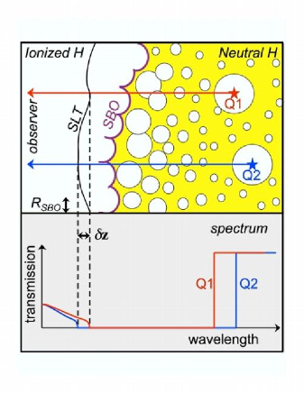
Figure 61: The distances to the observed Surface of Bubble Overlap (SBO) and Surface of Ly$\alpha$ Transmission (SLT) fluctuate on the sky. The SBO corresponds to the first region of diffuse neutral IGM observed along a random line-of-sight. It fluctuates across a shell with a minimum width dictated by the condition that the light crossing time across the characteristic radius $R_{\rm SBO}$ of ionized bubbles equals the cosmic scatter in their formation times. Thus, causality and cosmic variance determine the characteristic scale of bubbles at the completion of bubble overlap. After some time delay the IGM becomes transparent to Ly$\alpha$ photons, resulting in a second surface, the SLT. The upper panel illustrates how the lines-of-sight towards two quasars (Q1 in red and Q2 in blue) intersect the SLT with a redshift difference $\delta z$. The resulting variation in the observed spectrum of the two quasars is shown in the lower panel. Observationally, the ensemble of redshifts down to which the Gunn-Peterson troughs are seen in the spectra of $z>6.1$ quasars is drawn from the probability distribution $dP/dz_{\rm SLT}$ for the redshift at which the IGM started to allow Ly$\alpha$ transmission along random lines-of-sight. The observed values of $z_{\rm SLT}$ show a small scatterf2 in the SLT redshift around an average value of $\langle z_{\rm SLT}\rangle\approx 5.95$. Some regions of the IGM may have also become transparent to Ly$\alpha$ photons prior to overlap, resulting in windows of transmission inside the Gunn-Peterson trough (one such region may have been seenWB1 in SDSS J1148+5251). In the existing examples, the portions of the Universe probed by the lower end of the Gunn-Peterson trough are located several hundred comoving Mpc away from the background quasar, and are therefore not correlated with the quasar host galaxy. The distribution $dP/dz_{\rm SLT}$ is also independent of the redshift distribution of the quasars. Moreover, lines-of-sight to these quasars are not causally connected at $z\sim 6$ and may be considered independent.

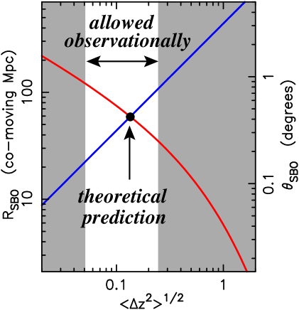
Figure 62: Constraints on the scatter in the SBO redshift and the characteristic size of isolated bubbles at the final overlap stage, $R_{\rm SBO}$ (see Fig. 1). The characteristic size of H II regions grows with time. The SBO is observed for the bubble scale at which the light crossing time (blue line) first becomes smaller than the cosmic scatter in bubble formation times (red line). At $z\sim 6$, the implied scale $R_{\rm SBO}\sim 60$ comoving Mpc (or $\sim 8.6$ physical Mpc), corresponds to a characteristic angular radius of $\theta_{\rm SLT}\sim 0.4$ degrees on the sky. After bubble overlap, the ionizing intensity grows to a level at which the IGM becomes transparent to Ly$\alpha$ photons. The collapsed fraction required for Ly$\alpha$ transmission within a region of a certain size will be larger than required for its ionization. However, the scatter in equation (174) is not sensitive to the collapsed fraction, and so may be used for both the SBO and SLT. The scatter in the SLT is smaller than the cosmic scatter in the structure formation time on the scale of the mean-free-path for ionizing photons. This mean-free-path must be longer than $R_{\rm SBO}\sim 60$Mpc, an inference which is supported by analysis of the Ly$\alpha$ forest at $z\sim 4$ where the mean-free-path is estimatedME1 to be $\sim 120$ comoving Mpc at the Lyman limit (and longer at higher frequencies). If it is dominated by cosmic variance, then the scatter in the SLT redshift provides a lower limit to the SBO scatter. The three known quasars at $z>6.1$ have Ly$\alpha$ transmission redshifts ofWB1 ; f2 $z_{\rm SLT}=5.9$, 5.95 and 5.98, implying that the scatter in the SBO must be $>0.05$ (this scatter may become better known from follow-up spectroscopy of Gamma Ray Burst afterglows at $z>6$ that might be discovered by the SWIFT satelliteGRBquasar ; BL02 ). The observed scatter in the SLT redshift is somewhat smaller than the predicted SBO scatter, confirming the expectation that cosmic variance is smaller at the SLT. The scatter in the SBO redshift must also be $<0.25$ because the lines-of-sight to the two highest redshift quasars have a redshift of Ly$\alpha$ transparency at $z\sim 6$, but a neutral fraction that is known from the proximity effectWL04b to be substantial at $z>6.2-6.3$. The excluded regions of scatter for the SBO are shown in gray.

The full size distribution of ionized bubbles has to be calculated from a numerical cosmological simulation that includes gas dynamics and radiative transfer. The simulation box needs to be sufficiently large for it to sample an unbiased volume of the Universe with little cosmic variance, but at the same time one must resolve the scale of individual dwarf galaxies which provide (as well as consume) ionizing photons (see discussion at the last section of this review). Until a reliable simulation of this magnitude exists, one must adopt an approximate analytic approach to estimate the bubble size distribution. Below we describe an example for such a method, developed by Furlanetto, Zaldarriaga, & Hernquist (2004) FZH .

The criterion for a region to be ionized is that galaxies inside of it produce a sufficient number of ionizing photons per baryon. This condition can be translated to the requirement that the collapsed fraction of mass in halos above some threshold mass $M_{\rm min}$ will exceed some threshold, namely $F_{\rm col}>\zeta^{-1}$. The minimum halo mass most likely corresponds to a virial temperature of $10^{4}$K relating to the threshold for atomic cooling (assuming that molecular hydrogen cooling is suppressed by the UV background in the Lyman-Werner band). We would like to find the largest region around every point that satisfies the above condition on the collapse fraction and then calculate the abundance of ionized regions of this size. Different regions have different values of $F_{\rm col}$ because their mean density is different. In the extended Press-Schechter model (Bond et al. 1991 bond91 ; Lacey & Cole 1993 LC93 ), the collapse fraction in a region of mean overdensity $\delta_{M}$ is

$$F_{\rm col}={\rm erfc}\left({\delta_{c}-\delta_{M}\over\sqrt{2[\sigma_{\rm min}^{2}-\sigma^{2}(M,z)]}}\right).$$ (175)

where $\sigma^{2}(M,z)$ is the variance of density fluctuations on mass scale $M$, $\sigma^{2}_{\rm min}\equiv\sigma^{2}(M_{\rm min},z)$, and $\delta_{c}$ is the collapse threshold. This equation can be used to derive the condition on the mean overdensity within a region of mass $M$ in order for it to be ionized,

$$\delta_{M}>\delta_{B}(M,z)\equiv\delta_{c}-{\sqrt{2}}K(\zeta)[\sigma_{\rm min}^{2}-\sigma^{2}(M,z)]^{1/2},$$ (176)

where $K(\zeta)={\rm erfc}^{-1}(1-\zeta^{-1})$. Furlanetto et al. FZH showed how to construct the mass function of ionized regions from $\delta_{B}$ in analogy with the halo mass function (Press & Schechter 1974 Press ; Bond et al. 1991 bond91 ). The barrier in equation (176) is well approximated by a linear dependence on $\sigma^{2}$,

$$\delta_{B}\approx B(M)=B_{0}+B_{1}\sigma^{2}(M),$$ (177)

in which case the mass function has an analytic solution (Sheth 1998 sheth98 ),

$$n(M)={\sqrt{2\over\pi}}{{\bar{\rho}}\over M^{2}}\left|{d\ln\sigma\over d\ln M}\right|{B_{0}\over\sigma(M)}\exp\left[-{B^{2}(M)\over 2\sigma^{2}(M)}\right],$$ (178)

where ${\bar{\rho}}$ is the mean mass density. This solution provides the comoving number density of ionized bubbles with mass in the range of $(M,M+dM)$. The main difference of this result from the Press-Schechter mass function is that the barrier in this case becomes more difficult to cross on smaller scales because $\delta_{B}$ is a decreasing function of mass $M$. This gives bubbles a characteristic size. The size evolves with redshift in a way that depends only on $\zeta$ and $M_{\rm min}$.

One limitation of the above analytic model is that it ignores the non-local influence of sources on distant regions (such as voids) as well as the possible shadowing effect of intervening gas. Radiative transfer effects in the real Universe are inherently three-dimensional and cannot be fully captured by spherical averages as done in this model. Moreover, the value of $M_{\rm min}$ is expected to increase in regions that were already ionized, complicating the expectation of whether they will remain ionized later. The history of reionization could be complicated and non monotonic in individual regions, as described by Furlanetto & Loeb (2005) FL05 . Finally, the above analytic formalism does not take the light propagation delay into account as we have done above in estimating the characteristic bubble size at the end of reionization. Hence this formalism describes the observed bubbles only as long as the characteristic bubble size is sufficiently small, so that the light propagation delay can be neglected compared to cosmic variance. The general effect of the light propagation delay on the power-spectrum of 21cm fluctuations was quantified by Barkana & Loeb (2005) BLinf .

9.3 Separating the “Physics” from the “Astrophysics” of the Reionization Epoch with 21cm Fluctuations

The 21cm signal can be seen from epochs during which the cosmic gas was largely neutral and deviated from thermal equilibrium with the cosmic microwave background (CMB). The signal vanished at redshifts $z>200$, when the residual fraction of free electrons after cosmological recombination kept the gas kinetic temperature, $T_{k}$, close to the CMB temperature, $T_{\gamma}$. But during $200>z>30$ the gas cooled adiabatically and atomic collisions kept the spin temperature of the hyperfine level population below $T_{\gamma}$, so that the gas appeared in absorption Scott ; Loeb04 . As the Hubble expansion continued to rarefy the gas, radiative coupling of $T_{s}$ to $T_{\gamma}$ began to dominate and the 21cm signal faded. When the first galaxies formed, the UV photons they produced between the Ly$\alpha$ and Lyman limit wavelengths propagated freely through the Universe, redshifted into the Ly$\alpha$ resonance, and coupled $T_{s}$ and $T_{k}$ once again through the Wouthuysen-Field Wout ; Field effect by which the two hyperfine states are mixed through the absorption and re-emission of a Ly$\alpha$ photon (Madau, ; Ciardi, ). Emission above the Lyman limit by the same galaxies initiated the process of reionization by creating ionized bubbles in the neutral cosmic gas, while X-ray photons propagated farther and heated $T_{k}$ above $T_{\gamma}$ throughout the Universe. Once $T_{s}$ grew larger than $T_{\gamma}$, the gas appeared in 21cm emission. The ionized bubbles imprinted a knee in the power spectrum of 21cm fluctuations (Zalda04, ), which traced the H I topology until the process of reionization was completed (FZH, ).

The various effects that determine the 21cm fluctuations can be separated into two classes. The density power spectrum probes basic cosmological parameters and inflationary initial conditions, and can be calculated exactly in linear theory. However, the radiation from galaxies, both Ly$\alpha$ radiation and ionizing photons, involves the complex, non-linear physics of galaxy formation and star formation. If only the sum of all fluctuations could be measured, then it would be difficult to extract the separate sources, and in particular, the extraction of the power spectrum would be subject to systematic errors involving the properties of galaxies. Barkana & Loeb (2005) BL05a showed that the unique three-dimensional properties of 21cm measurements permit a separation of these distinct effects. Thus, 21cm fluctuations can probe astrophysical (radiative) sources associated with the first galaxies, while at the same time separately probing the physical (inflationary) initial conditions of the Universe. In order to affect this separation most easily, it is necessary to measure the three-dimensional power spectrum of 21cm fluctuations. The discussion in this section follows Barkana & Loeb (2005) BL05a .

Spin temperature history

As long as the spin-temperature $T_{s}$ is smaller than the CMB temperature $T_{\gamma}=2.725(1+z)$ K, hydrogen atoms absorb the CMB, whereas if $T_{s}>T_{\gamma}$ they emit excess flux. In general, the resonant 21cm interaction changes the brightness temperature of the CMB by (Scott, ; Madau, ) $T_{b}=\tau\left(T_{s}-T_{\gamma}\right)/(1+z)$, where the optical depth at a wavelength $\lambda=21$cm is

$$\tau=\frac{3c\lambda^{2}hA_{10}n_{\rm H}}{32\pi kT_{s}\,(1+z)\,(dv_{r}/dr)}x_{\rm HI}\ ,$$ (179)

where $n_{H}$ is the number density of hydrogen, $A_{10}=2.85\times 10^{-15}~{}{\rm s^{-1}}$ is the spontaneous emission coefficient, $x_{\rm HI}$ is the neutral hydrogen fraction, and $dv_{r}/dr$ is the gradient of the radial velocity along the line of sight with $v_{r}$ being the physical radial velocity and $r$ the comoving distance; on average $dv_{r}/dr=H(z)/(1+z)$ where $H$ is the Hubble parameter. The velocity gradient term arises because it dictates the path length over which a 21cm photon resonates with atoms before it is shifted out of resonance by the Doppler effect (Sobolev, ).

For the concordance set of cosmological parameters (WMAP, ), the mean brightness temperature on the sky at redshift $z$ is

$$T_{b}=28\,{\rm mK}\,\left(\frac{\Omega_{b}h}{.033}\right)\left(\frac{\Omega_{m}}{.27}\right)^{-\frac{1}{2}}\left[{({1+z})\over{10}}\right]^{1/2}\left[{({T_{s}-T_{\gamma}})\over{T_{s}}}\right]\bar{x}_{\rm HI},$$ (180)

where $\bar{x}_{\rm HI}$ is the mean neutral fraction of hydrogen. The spin temperature itself is coupled to $T_{k}$ through the spin-flip transition, which can be excited by collisions or by the absorption of Ly$\alpha$ photons. As a result, the combination that appears in $T_{b}$ becomes (Field, ) $(T_{s}-T_{\gamma})/T_{s}=[x_{\rm tot}/(1+x_{\rm tot})]\left(1-T_{\gamma}/T_{k}\right)$, where $x_{\rm tot}=x_{\alpha}+x_{c}$ is the sum of the radiative and collisional threshold parameters. These parameters are $x_{\alpha}={4P_{\alpha}T_{\star}}/{27A_{10}T_{\gamma}}$ and $x_{c}={4\kappa_{1-0}(T_{k})\,n_{H}T_{\star}}/{3A_{10}T_{\gamma}}$, where $P_{\alpha}$ is the Ly$\alpha$ scattering rate which is proportional to the Ly$\alpha$ intensity, and $\kappa_{1-0}$ is tabulated as a function of $T_{k}$ (AD, ; Zyg, ). The coupling of the spin temperature to the gas temperature becomes substantial when $x_{\rm tot}>1$.

Brightness temperature fluctuations

Although the mean 21cm emission or absorption is difficult to measure due to bright foregrounds, the unique character of the fluctuations in $T_{b}$ allows for a much easier extraction of the signal (Shaver, ; Zalda04, ; Miguel1, ; Miguel2, ; Santos, ). We adopt the notation $\delta_{A}$ for the fractional fluctuation in quantity $A$ (with a lone $\delta$ denoting density perturbations). In general, the fluctuations in $T_{b}$ can be sourced by fluctuations in gas density ($\delta$), Ly$\alpha$ flux (through $\delta_{x_{\alpha}}$) neutral fraction ($\delta_{x_{\rm HI}}$), radial velocity gradient ($\delta_{d_{r}v_{r}}$), and temperature, so we find

$$\delta_{T_{b}} = \left(1+\frac{x_{c}}{\tilde{x}_{\rm tot}}\right)\delta+\frac{x_{\alpha}}{\tilde{x}_{\rm tot}}\delta_{x_{\alpha}}+\delta_{x_{\rm HI}}-\delta_{d_{r}v_{r}}$$ (181)

$$+(\gamma_{a}-1)\left[\frac{T_{\gamma}}{T_{k}-T_{\gamma}}+\frac{x_{c}}{\tilde{x}_{\rm tot}}\,\frac{d\log(\kappa_{1-0})}{d\log(T_{k})}\right]\,\delta\ ,$$

where the adiabatic index is $\gamma_{a}=1+(\delta_{T_{k}}/\delta)$, and we define $\tilde{x}_{\rm tot}\equiv(1+x_{\rm tot})x_{\rm tot}$. Taking the Fourier transform, we obtain the power spectrum of each quantity; e.g., the total power spectrum $P_{T_{b}}$ is defined by

$$\langle{\tilde{\delta}}_{T_{b}}({\bf k}_{1}){\tilde{\delta}}_{T_{b}}({\bf k}_{2})\rangle=(2\pi)^{3}\delta^{D}({\bf k}_{1}+{\bf k}_{2})P_{T_{b}}({\bf k}_{1})\ ,$$ (182)

where ${\tilde{\delta}}_{T_{b}}({\bf k})$ is the Fourier transform of $\delta_{T_{b}}$, ${\bf k}$ is the comoving wavevector, $\delta^{D}$ is the Dirac delta function, and $\langle\cdots\rangle$ denotes an ensemble average. In this analysis, we consider scales much bigger than the characteristic bubble size and the early phase of reionization (when ${\bar{\delta_{x_{\rm HI}}}}<<1$), so that the fluctuations $\delta_{x_{\rm HI}}$ are also much smaller than unity. For a more general treatment, see McQuinn et al. (2005) McQuinn .

The separation of powers

The fluctuation $\delta_{T_{b}}$ consists of a number of isotropic sources of fluctuations plus the peculiar velocity term $-\delta_{d_{r}v_{r}}$. Its Fourier transform is simply proportional to that of the density field (kaiser, ; Indian, ),

$${\tilde{\delta}}_{d_{r}v_{r}}=-\mu^{2}{\tilde{\delta}},$$ (183)

where $\mu=\cos\theta_{k}$ in terms of the angle $\theta_{k}$ of ${\bf k}$ with respect to the line of sight. The $\mu^{2}$ dependence in this equation results from taking the radial (i.e., line-of-sight) component ($\propto\mu$) of the peculiar velocity, and then the radial component ($\propto\mu$) of its gradient. Intuitively, a high-density region possesses a velocity infall towards the density peak, implying that a photon must travel further from the peak in order to reach a fixed relative redshift, compared with the case of pure Hubble expansion. Thus the optical depth is always increased by this effect in regions with $\delta>0$. This phenomenon is most properly termed velocity compression.

We therefore write the fluctuation in Fourier space as

$${\tilde{\delta}}_{T_{b}}({\bf k})=\mu^{2}{\tilde{\delta}}({\bf k})+\beta{\tilde{\delta}}({\bf k})+{\tilde{\delta}}_{\rm rad}({\bf k})\ ,$$ (184)

where we have defined a coefficient $\beta$ by collecting all terms $\propto\delta$ in Eq. (181), and have also combined the terms that depend on the radiation fields of Ly$\alpha$ photons and ionizing photons, respectively. We assume that these radiation fields produce isotropic power spectra, since the physical processes that determine them have no preferred direction in space. The total power spectrum is

$$P_{T_{b}}({\bf k}) = \mu^{4}P_{\delta}(k)+2\mu^{2}[\beta P_{\delta}(k)+P_{\delta\cdot{\rm rad}}(k)]+$$ (185)

$$[\beta^{2}P_{\delta}(k)+P_{\rm rad}(k)+2\beta P_{\delta\cdot{\rm rad}}(k)]\ ,$$

where we have defined the power spectrum $P_{\delta\cdot{\rm rad}}$ as the Fourier transform of the cross-correlation function,

$$\xi_{\delta\cdot{\rm rad}}(r)=\langle\delta({\bf r}_{1})\,\delta_{\rm rad}({\bf r}_{1}+{\bf r})\rangle\ .$$ (186)

We note that a similar anisotropy in the power spectrum has been previously derived in a different context, i.e., where the use of galaxy redshifts to estimate distances changes the apparent line-of-sight density of galaxies in redshift surveys (kaiser, ; lilje, ; hamilton, ; fisher, ). However, galaxies are intrinsically complex tracers of the underlying density field, and in that case there is no analog to the method that we demonstrate below for separating in 21cm fluctuations the effect of initial conditions from that of later astrophysical processes.

The velocity gradient term has also been examined for its global effect on the sky-averaged power and on radio visibilities (t00, ; Indian, ). The other sources of 21cm perturbations are isotropic and would produce a power spectrum $P_{T_{b}}(k)$ that could be measured by averaging the power over spherical shells in ${\bf k}$ space. In the simple case where $\beta=1$ and only the density and velocity terms contribute, the velocity term increases the total power by a factor of $\langle(1+\mu^{2})^{2}\rangle=1.87$ in the spherical average. However, instead of averaging the signal, we can use the angular structure of the power spectrum to greatly increase the discriminatory power of 21cm observations. We may break up each spherical shell in ${\bf k}$ space into rings of constant $\mu$ and construct the observed $P_{T_{b}}(k,\mu)$. Considering Eq. (185) as a polynomial in $\mu$, i.e., $\mu^{4}P_{\mu^{4}}+\mu^{2}P_{\mu^{2}}+P_{\mu^{0}}$, we see that the power at just three values of $\mu$ is required in order to separate out the coefficients of 1, $\mu^{2}$, and $\mu^{4}$ for each $k$.

If the velocity compression were not present, then only the $\mu$-independent term (times $T_{b}^{2}$) would have been observed, and its separation into the five components ($T_{b}$, $\beta$, and three power spectra) would have been difficult and subject to degeneracies. Once the power has been separated into three parts, however, the $\mu^{4}$ coefficient can be used to measure the density power spectrum directly, with no interference from any other source of fluctuations. Since the overall amplitude of the power spectrum, and its scaling with redshift, are well determined from the combination of the CMB temperature fluctuations and galaxy surveys, the amplitude of $P_{\mu^{4}}$ directly determines the mean brightness temperature $T_{b}$ on the sky, which measures a combination of $T_{s}$ and $\bar{x}_{\rm HI}$ at the observed redshift. McQuinn et al. (2005) McQuinn analysed in detail the parameters that can be constrained by upcoming 21cm experiments in concert with future CMB experiments such as Planck (http://www.rssd.esa.int/index.php?project=PLANCK). Once $P_{\delta}(k)$ has been determined, the coefficients of the $\mu^{2}$ term and the $\mu$-independent term must be used to determine the remaining unknowns, $\beta$, $P_{\delta\cdot{\rm rad}}(k)$, and $P_{\rm rad}(k)$. Since the coefficient $\beta$ is independent of $k$, determining it and thus breaking the last remaining degeneracy requires only a weak additional assumption on the behavior of the power spectra, such as their asymptotic behavior at large or small scales. If the measurements cover $N_{k}$ values of wavenumber $k$, then one wishes to determine $2N_{k}+1$ quantities based on $2N_{k}$ measurements, which should not cause significant degeneracies when $N_{k}\gg 1$. Even without knowing $\beta$, one can probe whether some sources of $P_{\rm rad}(k)$ are uncorrelated with $\delta$; the quantity $P_{\rm un-\delta}(k)\equiv P_{\mu^{0}}-P_{\mu^{2}}^{2}/(4P_{\mu^{4}})$ equals $P_{\rm rad}-P_{\delta\cdot{\rm rad}}^{2}/P_{\delta}$, which receives no contribution from any source that is a linear functional of the density distribution (see the next subsection for an example).

Specific epochs

At $z\sim 35$, collisions are effective due to the high gas density, so one can measure the density power spectrum (Loeb04, ) and the redshift evolution of $n_{\rm HI}$, $T_{\gamma}$, and $T_{k}$. At $z<35$, collisions become ineffective but the first stars produce a cosmic background of Ly$\alpha$ photons (i.e. photons that redshift into the Ly$\alpha$ resonance) that couples $T_{s}$ to $T_{k}$. During the period of initial Ly$\alpha$ coupling, fluctuations in the Ly$\alpha$ flux translate into fluctuations in the 21cm brightness (BarkL05, ). This signal can be observed from $z\sim 25$ until the Ly$\alpha$ coupling is completed (i.e., $x_{\rm tot}\gg 1$) at $z\sim 15$. At a given redshift, each atom sees Ly$\alpha$ photons that were originally emitted at earlier times at rest-frame wavelengths between Ly$\alpha$ and the Lyman limit. Distant sources are time retarded, and since there are fewer galaxies in the distant, earlier Universe, each atom sees sources only out to an apparent source horizon of $\sim 100$ comoving Mpc at $z\sim 20$. A significant portion of the flux comes from nearby sources, because of the $1/r^{2}$ decline of flux with distance, and since higher Lyman series photons, which are degraded to Ly$\alpha$ photons through scattering, can only be seen from a small redshift interval that corresponds to the wavelength interval between two consecutive atomic levels.

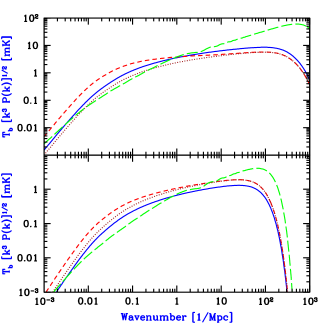
Figure 63: Observable power spectra during the period of initial Ly$\alpha$ coupling. Upper panel: Assumes adiabatic cooling. Lower panel: Assumes pre-heating to 500 K by X-ray sources. Shown are $P_{\mu^{4}}=P_{\delta}$ (solid curves), $P_{\mu^{2}}$ (short-dashed curves), and $P_{\rm un-\delta}$ (long-dashed curves), as well as for comparison $2\beta P_{\delta}$ (dotted curves).

There are two separate sources of fluctuations in the Ly$\alpha$ flux (BarkL05, ). The first is density inhomogeneities. Since gravitational instability proceeds faster in overdense regions, the biased distribution of rare galactic halos fluctuates much more than the global dark matter density. When the number of sources seen by each atom is relatively small, Poisson fluctuations provide a second source of fluctuations. Unlike typical Poisson noise, these fluctuations are correlated between gas elements at different places, since two nearby elements see many of the same sources. Assuming a scale-invariant spectrum of primordial density fluctuations, and that $x_{\alpha}=1$ is produced at $z=20$ by galaxies in dark matter halos where the gas cools efficiently via atomic cooling, Figure 63 shows the predicted observable power spectra. The figure suggests that $\beta$ can be measured from the ratio $P_{\mu^{2}}/P_{\mu^{4}}$ at $k>1$ Mpc^-1, allowing the density-induced fluctuations in flux to be extracted from $P_{\mu^{2}}$, while only the Poisson fluctuations contribute to $P_{\rm un-\delta}$. Each of these components probes the number density of galaxies through its magnitude, and the distribution of source distances through its shape. Measurements at $k>100$ Mpc^-1 can independently probe $T_{k}$ because of the smoothing effects of the gas pressure and the thermal width of the 21cm line.

After Ly$\alpha$ coupling and X-ray heating are both completed, reionization continues. Since $\beta=1$ and $T_{k}\gg T_{\gamma}$, the normalization of $P_{\mu^{4}}$ directly measures the mean neutral hydrogen fraction, and one can separately probe the density fluctuations, the neutral hydrogen fluctuations, and their cross-correlation.

Fluctuations on large angular scales

Full-sky observations must normally be analyzed with an angular and radial transform (FZH, ; Santos, ; Indian, ), rather than a Fourier transform which is simpler and yields more directly the underlying 3D power spectrum (Miguel1, ; Miguel2, ). The 21cm brightness fluctuations at a given redshift – corresponding to a comoving distance $r_{0}$ from the observer – can be expanded in spherical harmonics with expansion coefficients $a_{lm}(\nu)$, where the angular power spectrum is

$$C_{l}(r_{0}) = \langle|a_{lm}(\nu)|^{2}\rangle=4\pi\int\frac{k^{2}dk}{2\pi^{2}}\biggl{[}G_{l}^{2}(kr_{0})P_{\delta}(k)+$$ (187)

$$2P_{\delta\cdot{\rm rad}}(k)G_{l}(kr_{0})j_{l}(kr_{0})+P_{\rm rad}(k)j_{l}^{2}(kr_{0})\biggl{]}\ ,$$

with $G_{l}(x)\equiv J_{l}(x)+(\beta-1)j_{l}(x)$ and $J_{l}(x)$ being a linear combination of spherical Bessel functions (Indian, ).

In an angular transform on the sky, an angle of $\theta$ radians translates to a spherical multipole $l\sim 3.5/\theta$. For measurements on a screen at a comoving distance $r_{0}$, a multipole $l$ normally measures 3D power on a scale of $k^{-1}\sim\theta r_{0}\sim 35/l$ Gpc for $l\gg 1$, since $r_{0}\sim 10$ Gpc at $z>10$. This estimate fails at $l<100$, however, when we consider the sources of 21cm fluctuations. The angular projection implied in $C_{l}$ involves a weighted average (Eq. 187) that favors large scales when $l$ is small, but density fluctuations possess little large-scale power, and the $C_{l}$ are dominated by power around the peak of $kP_{\delta}(k)$, at a few tens of comoving Mpc.

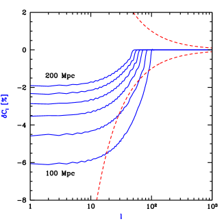
Figure 64: Effect of large-scale power on the angular power spectrum of 21cm anisotropies on the sky. This example shows the power from density fluctuations and velocity compression, assuming a warm IGM at $z=12$ with $T_{s}=T_{k}\gg T_{\gamma}$. Shown is the $\%$ change in $C_{l}$ if we were to cut off the power spectrum above $1/k$ of 200, 180, 160, 140, 120, and 100 Mpc (top to bottom). Also shown for comparison is the cosmic variance for averaging in bands of $\Delta l\sim l$ (dashed lines).

Figure 64 shows that for density and velocity fluctuations, even the $l=1$ multipole is affected by power at $k^{-1}>200$ Mpc only at the $2\%$ level. Due to the small number of large angular modes available on the sky, the expectation value of $C_{l}$ cannot be measured precisely at small $l$. Figure 64 shows that this precludes new information from being obtained on scales $k^{-1}>130$ Mpc using angular structure at any given redshift. Fluctuations on such scales may be measurable using a range of redshifts, but the required $\Delta z>1$ at $z\sim 10$ implies significant difficulties with foreground subtraction and with the need to account for time evolution.

10 Major Challenge for Future Theoretical Research: radiative transfer during reionization requires a large dynamic range, challenging the capabilities of existing simulation codes

Observations of the cosmic microwave background (WMAP, ) have confirmed the notion that the present large-scale structure in the Universe originated from small-amplitude density fluctuations at early cosmic times. Due to the natural instability of gravity, regions that were denser than average collapsed and formed bound halos, first on small spatial scales and later on larger and larger scales. At each snapshot of this cosmic evolution, the abundance of collapsed halos, whose masses are dominated by cold dark matter, can be computed from the initial conditions using numerical simulations and can be understood using approximate analytic models (ps74, ; bond91, ). The common understanding of galaxy formation is based on the notion that the constituent stars formed out of the gas that cooled and subsequently condensed to high densities in the cores of some of these halos (wr78, ).

The standard analytic model for the abundance of halos (ps74, ; bond91, ) considers the small density fluctuations at some early, initial time, and attempts to predict the number of halos that will form at some later time corresponding to a redshift $z$. First, the fluctuations are extrapolated to the present time using the growth rate of linear fluctuations, and then the average density is computed in spheres of various sizes. Whenever the overdensity (i.e., the density perturbation in units of the cosmic mean density) in a sphere rises above a critical threshold $\delta_{c}(z)$, the corresponding region is assumed to have collapsed by redshift $z$, forming a halo out of all the mass that had been included in the initial spherical region. In analyzing the statistics of such regions, the model separates the contribution of large-scale modes from that of small-scale density fluctuations. It predicts that galactic halos will form earlier in regions that are overdense on large scales (k84, ; b86, ; ck89, ; mw96, ), since these regions already start out from an enhanced level of density, and small-scale modes need only supply the remaining perturbation necessary to reach $\delta_{c}(z)$. On the other hand, large-scale voids should contain a reduced number of halos at high redshift. In this way, the analytic model describes the clustering of massive halos.

As gas falls into a dark matter halo, it can fragment into stars only if its virial temperature is above $10^{4}$K for cooling mediated by atomic transitions [or $\sim 500$ K for molecular ${\rm H}_{2}$ cooling; see Fig. 20]. The abundance of dark matter halos with a virial temperature above this cooling threshold declines sharply with increasing redshift due to the exponential cutoff in the abundance of massive halos at early cosmic times. Consequently, a small change in the collapse threshold of these rare halos, due to mild inhomogeneities on much larger spatial scales, can change the abundance of such halos dramatically. Barkana & Loeb (2004) BL04a have shown that the modulation of galaxy formation by long wavelength modes of density fluctuations is therefore amplified considerably at high redshift; the discussion in this section follows their analysis.

Amplification of Density Fluctuations

Galaxies at high redshift are believed to form in all halos above some minimum mass $M_{\rm min}$ that depends on the efficiency of atomic and molecular transitions that cool the gas within each halo. This makes useful the standard quantity of the collapse fraction $F_{\rm col}(M_{\rm min})$, which is the fraction of mass in a given volume that is contained in halos of individual mass $M_{\rm min}$ or greater (see Fig. 13). If we set $M_{\rm min}$ to be the minimum halo mass in which efficient cooling processes are triggered, then $F_{\rm col}(M_{\rm min})$ is the fraction of all baryons that reside in galaxies. In a large-scale region of comoving radius $R$ with a mean overdensity $\bar{\delta}_{R}$, the standard result is (bond91, )

$$F_{\rm col}(M_{\rm min})={\rm erfc}\left[\frac{\delta_{c}(z)-\bar{\delta}_{R}}{\sqrt{2\left[S(R_{\rm min})-S(R)\right]}}\right]\ ,$$ (188)

where $S(R)=\sigma^{2}(R)$ is the variance of fluctuations in spheres of radius $R$, and $S(R_{\rm min})$ is the variance in spheres of radius $R_{\rm min}$ corresponding to the region at the initial time that contained a mass $M_{\rm min}$. In particular, the cosmic mean value of the collapse fraction is obtained in the limit of $R\rightarrow\infty$ by setting $\bar{\delta}_{R}$ and $S(R)$ to zero in this expression. Throughout this section we shall adopt this standard model, known as the extended Press-Schechter model. Whenever we consider a cubic region, we will estimate its halo abundance by applying the model to a spherical region of equal volume. Note also that we will consistently quote values of comoving distance, which equals physical distance times a factor of $(1+z)$.

At high redshift, galactic halos are rare and correspond to high peaks in the Gaussian probability distribution of initial fluctuations. A modest change in the overall density of a large region modulates the threshold for high peaks in the Gaussian density field, so that the number of galaxies is exponentially sensitive to this modulation. This amplification of large-scale modes is responsible for the large statistical fluctuations that we find.

In numerical simulations, periodic boundary conditions are usually assumed, and this forces the mean density of the box to equal the cosmic mean density. The abundance of halos as a function of mass is then biased in such a box (see Fig. 65), since a similar region in the real Universe will have a distribution of different overdensities $\bar{\delta}_{R}$. At high redshift, when galaxies correspond to high peaks, they are mostly found in regions with an enhanced large-scale density. In a periodic box, therefore, the total number of galaxies is artificially reduced, and the relative abundance of galactic halos with different masses is artificially tilted in favor of lower-mass halos. Let us illustrate these results for two sets of parameters, one corresponding to the first galaxies and early reionization ($z=20$) and the other to the current horizon in observations of galaxies and late reionization ($z=7$). Let us consider a resolution equal to that of state-of-the-art cosmological simulations that include gravity and gas hydrodynamics. Specifically, let us assume that the total number of dark matter particles in the simulation is $N=324^{3}$, and that the smallest halo that can form a galaxy must be resolved into 500 particles; converge showed that this resolution is necessary in order to determine the star formation rate in an individual halo reliably to within a factor of two. Therefore, if we assume that halos that cool via molecular hydrogen must be resolved at $z=20$ (so that $M_{\rm min}=7\times 10^{5}M_{\odot}$), and only those that cool via atomic transitions must be resolved at $z=7$ (so that $M_{\rm min}=10^{8}M_{\odot}$), then the maximum box sizes that can currently be simulated in hydrodynamic comological simulations are $l_{\rm box}=1$ Mpc and $l_{\rm box}=6$ Mpc at these two redshifts, respectively.

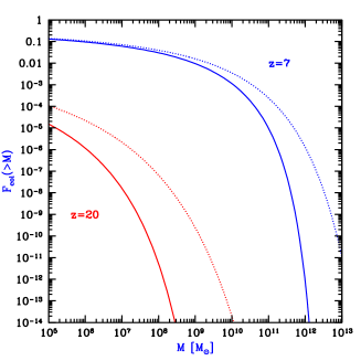
Figure 65: Bias in the halo mass distribution in simulations. Shown is the amount of mass contained in all halos of individual mass $M_{\rm min}$ or greater, expressed as a fraction of the total mass in a given volume. This cumulative fraction $F_{\rm col}(M_{\rm min})$ is illustrated as a function of the minimum halo mass $M_{\rm min}$. We consider two cases of redshift and simulation box size, namely $z=7$, $l_{\rm box}=6$ Mpc (upper curves), and $z=20$, $l_{\rm box}=1$ Mpc (lower curves). At each redshift, we compare the true average distribution in the Universe (dotted curve) to the biased distribution (solid curve) that would be measured in a simulation box with periodic boundary conditions (for which $\bar{\delta}_{R}$ is artificially set to zero).

At each redshift we only consider cubic boxes large enough so that the probability of forming a halo on the scale of the entire box is negligible. In this case, $\bar{\delta}_{R}$ is Gaussian distributed with zero mean and variance $S(R)$, since the no-halo condition $\sqrt{S(R)}\ll\delta_{c}(z)$ implies that at redshift $z$ the perturbation on the scale $R$ is still in the linear regime. We can then calculate the probability distribution of collapse fractions in a box of a given size (see Fig.66). This distribution corresponds to a real variation in the fraction of gas in galaxies within different regions of the Universe at a given time. In a numerical simulation, the assumption of periodic boundary conditions eliminates the large-scale modes that cause this cosmic scatter. Note that Poisson fluctuations in the number of halos within the box would only add to the scatter, although the variations we have calculated are typically the dominant factor. For instance, in our two standard examples, the mean expected number of halos in the box is 3 at $z=20$ and 900 at $z=7$, resulting in Poisson fluctuations of a factor of about 2 and 1.03, respectively, compared to the clustering-induced scatter of a factor of about 16 and 2 in these two cases.

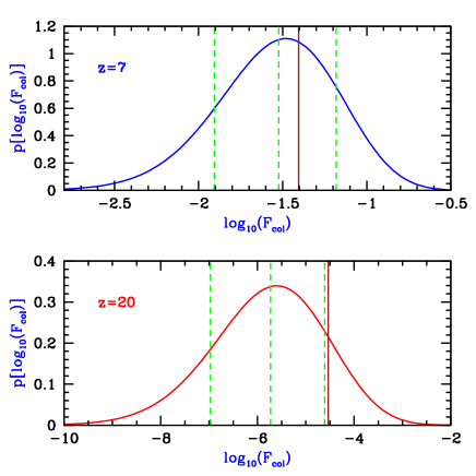
Figure 66: Probability distribution within a small volume of the total mass fraction in galactic halos. The normalized distribution of the logarithm of this fraction $F_{\rm col}(M_{\rm min})$ is shown for two cases: $z=7$, $l_{\rm box}=6$ Mpc, $M_{\rm min}=10^{8}M_{\odot}$ (upper panel), and $z=20$, $l_{\rm box}=1$ Mpc, $M_{\rm min}=7\times 10^{5}M_{\odot}$ (bottom panel). In each case, the value in a periodic box ($\bar{\delta}_{R}=0$) is shown along with the value that would be expected given a plus or minus $1-\sigma$ fluctuation in the mean density of the box (dashed vertical lines). Also shown in each case is the mean value of $F_{\rm col}(M_{\rm min})$ averaged over large cosmological volumes (solid vertical line).

Within the extended Press-Schechter model, both the numerical bias and the cosmic scatter can be simply described in terms of a shift in the redshift (see Fig. 67). In general, a region of radius $R$ with a mean overdensity $\bar{\delta}_{R}$ will contain a different collapse fraction than the cosmic mean value at a given redshift $z$. However, at some wrong redshift $z+\Delta z$ this small region will contain the cosmic mean collapse fraction at $z$. At high redshifts ($z>3$), this shift in redshift was derived by Barkana & Loeb BL04a from equation (188) [and was already mentioned in Eq. (174)]

$$\Delta z=\frac{\bar{\delta}_{R}}{\delta_{0}}-(1+z)\times\left[1-\sqrt{1-\frac{S(R)}{S(R_{\rm min})}}\ \right]\ ,$$ (189)

where $\delta_{0}\equiv\delta_{c}(z)/(1+z)$ is approximately constant at high redshifts (p80, ), and equals 1.28 for the standard cosmological parameters (with its deviation from the Einstein-de Sitter value of 1.69 resulting from the existence of a cosmological constant). Thus, in our two examples, the bias is -2.6 at $z=20$ and -0.4 at $z=7$, and the one-sided $1-\sigma$ scatter is 2.4 at $z=20$ and 1.2 at $z=7$.

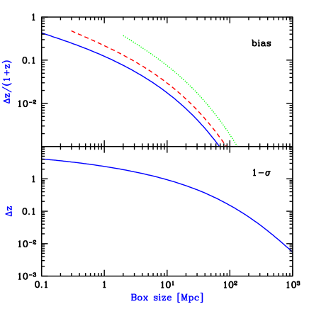
Figure 67: Cosmic scatter and numerical bias, expressed as the change in redshift needed to get the correct cosmic mean of the collapse fraction. The plot shows the $1-\sigma$ scatter (about the biased value) in the redshift of reionization, or any other phenomenon that depends on the mass fraction in galaxies (bottom panel), as well as the redshift bias [expressed as a fraction of $(1+z)$] in periodic simulation boxes (upper panel). The bias is shown for $M_{\rm min}=7\times 10^{5}M_{\odot}$ (solid curve), $M_{\rm min}=10^{8}M_{\odot}$ (dashed curve), and $M_{\rm min}=3\times 10^{10}M_{\odot}$ (dotted curve). The bias is always negative, and the plot gives its absolute value. When expressed as a shift in redshift, the scatter is independent of $M_{\rm min}$.

Matching Numerical Simulations

Next we may develop an improved model that fits the results of numerical simulations more accurately. The model constructs the halo mass distribution (or mass function); cumulative quantities such as the collapse fraction or the total number of galaxies can then be determined from it via integration. We first define $f(\delta_{c}(z),S)\,dS$ to be the mass fraction contained at $z$ within halos with mass in the range corresponding to $S$ to $S+dS$. As derived earlier, the Press-Schechter halo abundance is

$$\frac{dn}{dM}=\frac{\bar{\rho}_{0}}{M}\left|\frac{dS}{dM}\right|f(\delta_{c}(z),S)\ ,$$ (190)

where $dn$ is the comoving number density of halos with masses in the range $M$ to $M+dM$, and

$$f_{\rm PS}(\delta_{c}(z),S)=\frac{1}{\sqrt{2\pi}}\frac{\nu}{S}\exp\left[-\frac{\nu^{2}}{2}\right]\ ,$$ (191)

where $\nu=\delta_{c}(z)/\sqrt{S}$ is the number of standard deviations that the critical collapse overdensity represents on the mass scale $M$ corresponding to the variance $S$.

However, the Press-Schechter mass function fits numerical simulations only roughly, and in particular it substantially underestimates the abundance of the rare halos that host galaxies at high redshift. The halo mass function of shetht99 [see also shethmot ] adds two free parameters that allow it to fit numerical simulations much more accurately (jenkins, ). These N-body simulations followed very large volumes at low redshift, so that cosmic scatter did not compromise their accuracy. The matching mass function is given by

$$f_{\rm ST}(\delta_{c}(z),S)=A^{\prime}\frac{\nu}{S}\sqrt{\frac{a^{\prime}}{2\pi}}\left[1+\frac{1}{(a^{\prime}\nu^{2})^{q^{\prime}}}\right]\exp\left[-\frac{a^{\prime}\nu^{2}}{2}\right]\ ,$$ (192)

with best-fit parameters (shetht02, ) $a^{\prime}=0.75$ and $q^{\prime}=0.3$, and where normalization to unity is ensured by taking $A^{\prime}=0.322$.

In order to calculate cosmic scatter we must determine the biased halo mass function in a given volume at a given mean density. Within the extended Press-Schechter model (bond91, ), the halo mass distribution in a region of comoving radius $R$ with a mean overdensity $\bar{\delta}_{R}$ is given by

$$f_{\rm bias-PS}(\delta_{c}(z),\bar{\delta}_{R},R,S)=f_{\rm PS}(\delta_{c}(z)-\bar{\delta}_{R},S-S(R))\ .$$ (193)

The corresponding collapse fraction in this case is given simply by eq. (188). Despite the relatively low accuracy of the Press-Schechter mass function, the relative change is predicted rather accurately by the extended Press-Schechter model. In other words, the prediction for the halo mass function in a given volume compared to the cosmic mean mass function provides a good fit to numerical simulations over a wide range of parameters (mw96, ; casas02, ).

For the improved model (derived in BL04a ), we adopt a hybrid approach that combines various previous models with each applied where it has been found to closely match numerical simulations. We obtain the halo mass function within a restricted volume by starting with the Sheth-Torme formula for the cosmic mean mass function, and then adjusting it with a relative correction based on the extended Press-Schechter model. In other words, we set

$$f_{\rm bias}(\delta_{c}(z),\bar{\delta}_{R},R,S)=$$

$$f_{\rm ST}(\delta_{c}(z),S)\ \times\left[\frac{f_{\rm PS}(\delta_{c}(z)-\bar{\delta}_{R},S-S(R))}{f_{\rm PS}(\delta_{c}(z),S)}\right]\ .$$ (194)

As noted, this model is based on fits to simulations at low redshifts, but we can check it at high redshifts as well. Figure 68 shows the number of galactic halos at $z\sim 15-30$ in two numerical simulations run by yoshida , and our predictions given the cosmological input parameters assumed by each simulation. The close fit to the simulated data (with no additional free parameters) suggests that our hybrid model (solid lines) improves on the extended Press-Schechter model (dashed lines), and can be used to calculate accurately the cosmic scatter in the number of galaxies at both high and low redshifts. The simulated data significantly deviate from the expected cosmic mean [eq. (192), shown by the dotted line], due to the artificial suppression of large-scale modes outside the simulated box.

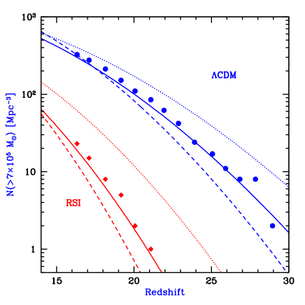
Figure 68: Halo mass function at high redshift in a 1 Mpc box at the cosmic mean density. The prediction (solid lines) of the hybrid model of Barkana & Loeb (2004) BL04a is compared with the number of halos above mass $7\times 10^{5}M_{\odot}$ measured in the simulations of yoshida [data points are taken from their Figure 5]. The cosmic mean of the halo mass function (dotted lines) deviates significantly from the simulated values, since the periodic boundary conditions within the finite simulation box artificially set the amplitude of large-scale modes to zero. The hybrid model starts with the Sheth-Tormen mass function and applies a correction based on the extended Press-Schechter model; in doing so, it provides a better fit to numerical simulations than the pure extended Press-Schechter model (dashed lines) used in the previous figures. We consider two sets of cosmological parameters, the scale-invariant $\Lambda$CDM model of yoshida (upper curves), and their running scalar index (RSI) model (lower curves).

As an additional example, we consider the highest-resolution first star simulation (ABN02, ), which used $l_{\rm box}=128$ kpc and $M_{\rm min}=7\times 10^{5}M_{\odot}$. The first star forms within the simulated volume when the first halo of mass $M_{\rm min}$ or larger collapses within the box. To compare with the simulation, we predict the redshift at which the probability of finding at least one halo within the box equals $50\%$, accounting for Poisson fluctuations. We find that if the simulation formed a population of halos corresponding to the correct cosmic average [as given by eq. (192)], then the first star should have formed already at $z=24.0$. The first star actually formed in the simulation box only at $z=18.2$ (ABN02, ). Using eq. (194) we can account for the loss of large-scale modes beyond the periodic box, and predict a first star at $z=17.8$, a close match given the large Poisson fluctuations introduced by considering a single galaxy within the box.

The artificial bias in periodic simulation boxes can also be seen in the results of extensive numerical convergence tests carried out by converge . They presented a large array of numerical simulations of galaxy formation run in periodic boxes over a wide range of box size, mass resolution, and redshift. In particular, we can identify several pairs of simulations where the simulations in each pair have the same mass resolution but different box sizes; this allows us to separate the effect of large-scale numerical bias from the effect of having poorly-resolved individual halos.

Implications

(i) The nature of reionization

A variety of papers in the literature (aw72, ; fk94, ; sgb94, ; hl97, ; g00, ; BL01, ; BL01a, ) maintain that reionization ended with a fast, simultaneous, overlap stage throughout the Universe. This view has been based on simple arguments and has been supported by numerical simulations with small box sizes. The underlying idea was that the ionized hydrogen (H II ) regions of individual sources began to overlap when the typical size of each H II bubble became comparable to the distance between nearby sources. Since these two length scales were comparable at the critical moment, there is only a single timescale in the problem – given by the growth rate of each bubble – and it determines the transition time between the initial overlap of two or three nearby bubbles, to the final stage where dozens or hundreds of individual sources overlap and produce large ionized regions. Whenever two ionized bubbles were joined, each point inside their common boundary became exposed to ionizing photons from both sources, reducing the neutral hydrogen fraction and allowing ionizing photons to travel farther before being absorbed. Thus, the ionizing intensity inside H II regions rose rapidly, allowing those regions to expand into high-density gas that had previously recombined fast enough to remain neutral when the ionizing intensity had been low. Since each bubble coalescence accelerates the process, it has been thought that the overlap phase has the character of a phase transition and occurs rapidly. Indeed, the simulations of reionization (g00, ) found that the average mean free path of ionizing photons in the simulated volume rises by an order of magnitude over a redshift interval $\Delta z=0.05$ at $z=7$.

These results imply that overlap is still expected to occur rapidly, but only in localized high-density regions, where the ionizing intensity and the mean free path rise rapidly even while other distant regions are still mostly neutral. In other words, the size of the bubble of an individual source is about the same in different regions (since most halos have masses just above $M_{\rm min}$), but the typical distance between nearby sources varies widely across the Universe. The strong clustering of ionizing sources on length scales as large as 30–100 Mpc introduces long timescales into the reionization phase transition. The sharpness of overlap is determined not by the growth rate of bubbles around individual sources, but by the ability of large groups of sources within overdense regions to deliver ionizing photons into large underdense regions.

Note that the recombination rate is higher in overdense regions because of their higher gas density. These regions still reionize first, though, despite the need to overcome the higher recombination rate, since the number of ionizing sources in these regions is increased even more strongly as a result of the dramatic amplification of large-scale modes discussed earlier.

(ii) Limitations of current simulations

The shortcomings of current simulations do not amount simply to a shift of $\sim 10\%$ in redshift and the elimination of scatter. The effect mentioned above can be expressed in terms of a shift in redshift only within the context of the extended Press-Schechter model, and only if the total mass fraction in galaxies is considered and not its distribution as a function of galaxy mass. The halo mass distribution should still have the wrong shape, resulting from the fact that $\Delta z$ depends on $M_{\rm min}$. A self-contained numerical simulation must directly evolve a very large volume.

Another reason that current simulations are limited is that at high redshift, when galaxies are still rare, the abundance of galaxies grows rapidly towards lower redshift. Therefore, a $\sim 10\%$ relative error in redshift implies that at any given redshift around $z\sim 10$–20, the simulation predicts a halo mass function that can be off by an order of magnitude for halos that host galaxies (see Fig. 68). This large underestimate suggests that the first generation of galaxies formed significantly earlier than indicated by recent simulations. Another element missed by simulations is the large cosmic scatter. This scatter can fundamentally change the character of any observable process or feedback mechanism that depends on a radiation background. Simulations in periodic boxes eliminate any large-scale scatter by assuming that the simulated volume is surrounded by identical periodic copies of itself. In the case of reionization, for instance, current simulations neglect the collective effects described above, whereby groups of sources in overdense regions may influence large surrounding underdense regions. In the case of the formation of the first stars due to molecular hydrogen cooling, the effect of the soft ultraviolet radiation from these stars, which tends to dissociate the molecular hydrogen around them (hrl97, ; rgs02, ; Oh03, ), must be reassessed with cosmic scatter included.

(iii) Observational consequences

The spatial fluctuations that we have calculated also affect current and future observations that probe reionization or the galaxy population at high redshift. For example, there are a large number of programs searching for galaxies at the highest accessible redshifts (6.5 and beyond) using their strong Ly$\alpha$ emission (h02, ; r03, ; m03, ; k03, ). These programs have previously been justified as a search for the reionization redshift, since the intrinsic emission should be absorbed more strongly by the surrounding IGM if this medium is neutral. For any particular source, it will be hard to clearly recognize this enhanced absorption because of uncertainties regarding the properties of the source and its radiative and gravitational effects on its surroundings (nature, ; GRBquasar, ; s03, ). However, if the luminosity function of galaxies that emit Ly$\alpha$ can be observed, then faint sources, which do not significantly affect their environment, should be very strongly absorbed in the era before reionization. Reionization can then be detected statistically through the sudden jump in the number of faint sourcesRhoads . The above results alter the expectation for such observations. Indeed, no sharp “reionization redshift” is expected. Instead, a Ly$\alpha$ luminosity function assembled from a large area of the sky will average over the cosmic scatter of $\Delta z\sim 1$–2 between different regions, resulting in a smooth evolution of the luminosity function over this redshift range. In addition, such a survey may be biased to give a relatively high redshift, since only the most massive galaxies can be detected, and as we have shown, these galaxies will be concentrated in overdense regions that will also get reionized relatively early.

The distribution of ionized patches during reionization will likely be probed by future observations, including small-scale anisotropies of the cosmic microwave background photons that are rescattered by the ionized patches (a96, ; gh98, ; san03, ), and observations of 21 cm emission by the spin-flip transition of the hydrogen in neutral regions (t00, ; cgo02, ; fsh03, ). Previous analytical and numerical estimates of these signals have not included the collective effects discussed above, in which rare groups of massive galaxies may reionize large surrounding areas. The transfer of photons across large scales will likely smooth out the signal even on scales significantly larger than the typical size of an H II bubble due to an individual galaxy. Therefore, even the characteristic angular scales that are expected to show correlations in such observations must be reassessed.

The cosmic scatter also affects observations in the present-day Universe that depend on the history of reionization. For instance, photoionization heating suppresses the formation of dwarf galaxies after reionization, suggesting that the smallest galaxies seen today may have formed prior to reionization (bkw01, ; s02, ; b02, ). Under the popular view that assumed a sharp end to reionization, it was expected that denser regions would have formed more galaxies by the time of reionization, possibly explaining the larger relative abundance of dwarf galaxies observed in galaxy clusters compared to lower-density regions such as the Local Group of galaxies (t02, ; b03, ). The above results undercut the basic assumption of this argument and suggest a different explanation. Reionization occurs roughly when the number of ionizing photons produced starts to exceed the number of hydrogen atoms in the surrounding IGM. If the processes of star formation and the production of ionizing photons are equally efficient within galaxies that lie in different regions, then reionization in each region will occur when the collapse fraction reaches the same critical value, even though this will occur at different times in different regions. Since the galaxies responsible for reionization have the same masses as present-day dwarf galaxies, this estimate argues for a roughly equal abundance of dwarf galaxies in all environments today. This simple picture is, however, modified by several additional effects. First, the recombination rate is higher in overdense regions at any given time, as discussed above. Furthermore, reionization in such regions is accomplished at an earlier time when the recombination rate was higher even at the mean cosmic density; therefore, more ionizing photons must be produced in order to compensate for the enhanced recombination rate. These two effects combine to make overdense regions reionize at a higher value of $F_{\rm col}$ than underdense regions. In addition, the overdense regions, which reionize first, subsequently send their extra ionizing photons into the surrounding underdense regions, causing the latter to reionize at an even lower $F_{\rm col}$. Thus, a higher abundance of dwarf galaxies today is indeed expected in the overdense regions.

The same basic effect may be even more critical for understanding the properties of large-scale voids, 10–30 Mpc regions in the present-day Universe with an average mass density that is well below the cosmic mean. In order to predict their properties, the first step is to consider the abundance of dark matter halos within them. Numerical simulations show that voids contain a lower relative abundance of rare halos (mw02, ; co00, ; bh03, ), as expected from the raising of the collapse threshold for halos within a void. On the other hand, simulations show that voids actually place a larger fraction of their dark matter content in dwarf halos of mass below $10^{10}M_{\odot}$ (gottl03, ). This can be understood within the extended Press-Schechter model. At the present time, a typical region in the Universe fills halos of mass $10^{12}M_{\odot}$ and higher with most of the dark matter, and very little is left over for isolated dwarf halos. Although a large number of dwarf halos may have formed at early times in such a region, the vast majority later merged with other halos, and by the present time they survive only as substructure inside much larger halos. In a void, on the other hand, large halos are rare even today, implying that most of the dwarf halos that formed early within a void can remain as isolated dwarf halos till the present. Thus, most isolated dwarf dark matter halos in the present Universe should be found within large-scale voids (infall, ).

However, voids are observed to be rather deficient in dwarf galaxies as well as in larger galaxies on the scale of the Milky Way mass of $\sim 10^{12}M_{\odot}$ BigVoid ; el-ad ; pVoids . A deficit of large galaxies is naturally expected, since the total mass density in the void is unusually low, and the fraction of this already low density that assembles in large halos is further reduced relative to higher-density regions. The absence of dwarf galaxies is harder to understand, given the higher relative abundance expected for their host dark matter halos. The standard model for galaxy formation may be consistent with the observations if some of the dwarf halos are dark and do not host stars. Large numbers of dark dwarf halos may be produced by the effect of reionization in suppressing the infall of gas into these halos. Indeed, exactly the same factors considered above, in the discussion of dwarf galaxies in clusters compared to those in small groups, apply also to voids. Thus, the voids should reionize last, but since they are most strongly affected by ionizing photons from their surroundings (which have a higher density than the voids themselves), the voids should reionize when the abundance of galaxies within them is relatively low.

Acknowledgements

I thank my young collaborators with whom my own research in this field was accomplished: Dan Babich, Rennan Barkana, Volker Bromm, Benedetta Ciardi, Daniel Eisenstein, Steve Furlanetto, Zoltan Haiman, Rosalba Perna, Stuart Wyithe, and Matias Zaldarriaga. I thank Donna Adams for her highly professional assistance with the latex file, and Dan Babich & Matt McQuinn for their helpful comments on the manuscript.

References

- (1) T. Abel, & M. G. Haehnelt: ApJ 520, 13 (1999)
- (2) T. Abel, M. L. Norman, & P. Madau: ApJ 523, 66 (1999)
- (3) T. Abel, & H. J. Mo: ApJ 494, L151 (1998)
- (4) T. Abel, G. Bryan, & M. Norman: ApJ, 540, 39 (2000)
- (5) T. Abel, G. L. Bryan, M. L. Norman: Science 295, 93 (2002)
- (6) K. L. Adelberger, & C. C. Steidel: ApJ 544, 218 (2000)
- (7) K. A. Adelberger, et al.: ApJ 584, 45 (2003)
- (8) N. Aghanim, F. X. Desert, J. L. Puget, & R. Gispert: A&A 311, 1 (1996)
- (9) A. Aguirre, L. Hernquist, D. Weinberg, N. Katz, & J. Gardner: ApJ 560, 599 (2001)
- (10) A. Aguirre, L. Hernquist, N. Katz, J. Gardner, & D. Weinberg: ApJ 556, L11 (2001)
- (11) A. C. Allison, & A. Dalgarno: ApJ 158, 423 (1969)
- (12) M. A. Alvarez, V. Bromm, & P. R. Shapiro: ApJ, in press (2006), (astro-ph/0507684)
- (13) J. Arons, & D. W. Wingert: ApJ 177, 1 (1972)
- (14) D. Babich, & A. Loeb: ApJ, in press (2006), (astro-ph/0509784)
- (15) A. Babul, & S. D. M. White: MNRAS 253, P31 (1991)
- (16) E. A. Baltz: arXiv:(astro-ph/0412170)
- (17) E. A. Baltz, N. Y. Gnedin, & J. Silk: ApJl 493, L1 (1998)
- (18) I. Baraffe, A. Heger, & S. E. Woosley: ApJ 550, 890 (2001)
- (19) J. M. Bardeen, J. R. Bond, N. Kaiser, & A. S. Szalay: ApJ 304, 15 (1986)
- (20) A. J. Barger, et al.: ApJ 584, L61 (2003)
- (21) R. Barkana, Z. Haiman, & J. P. Ostriker: ApJ 558, 482 (2001)
- (22) R. Barkana, & A. Loeb: ApJ 523, 54 (1999)
- (23) R. Barkana, & A. Loeb: Phys. Rep. 349, 125 (2001)
- (24) R. Barkana, & A. Loeb: Nature 421, 341 (2003)
- (25) R. Barkana: MNRAS 347, 57 (2004)
- (26) R. Barkana, & A. Loeb: ApJ 601, 64 (2004)
- (27) R. Barkana, & A. Loeb: ApJ, 609, 474 (2004)
- (28) R. Barkana, & A. Loeb: ApJ 624, L65 (2005)
- (29) R. Barkana, & A. Loeb: MNRAS, 363, L36 (2005)
- (30) R. Barkana, & A. Loeb: ApJ 626, 1 (2005)
- (31) M. R. Bate, I. A. Bonnell, & V. Bromm: MNRAS 332, L65 (2002)
- (32) M. R. Bate, I. A. Bonnell, & V. Bromm: MNRAS 339, 577 (2003)
- (33) M. Battaglia, A. De Roeck, J. R. Ellis, F. Gianotti, K. A. Olive and L. Pape: Eur. Phys. J. C 33, 273 (2004) [arXiv:hep-ph/0306219].
- (34) M. C. Begelman, R. D. Blandford, M. J. Rees: Rev. Mod. Phys. 56, 255 (1984)
- (35) M. Begelman, M. Ruszkowski: Phil.Trans.Roy.Soc.Lond. A363, 655 (2005)
- (36) C. L. Bennett, et al: ApJ 464, L1 (1996)
- (37) A. J.Benson, C. S. Frenk, C. G. Lacey, C. M. Baugh, & S. Cole: MNRAS 333, 177 (2002)
- (38) A. J. Benson, C. S. Frenk, C. M. Baugh, S. Cole, C. G. Lacey: MNRAS 343, 679 (2003)
- (39) A. J. Benson, F. Hoyle, F. Torres, & M. S. Vogeley: MNRAS 340, 160 (2003)
- (40) E. Bertschinger: ApJS 58, 39 (1985)
- (41) S. Bharadwaj & S. S. Ali: MNRAS 352, 142 (2004); 356, 1519 (2005)
- (42) S. Bianchi, A. Ferrara, J. I. Davies, P. B. Alton: MNRAS 311, 601 (2000)
- (43) J. Binney, & S. Tremaine: Galactic Dynamics (Princeton: Princeton Univ. Press) (1987)
- (44) G.D. Birkhoff: Relativity and Modern Physics. Cambridge: Harvard Univ. Press (1923)
- (45) A. W. Blain, & P. Natarajan: MNRAS 312, L35 (2000)
- (46) J. Bland-Hawthorn, & P. R. Maloney: ApJ 510, L33 (1999)
- (47) J. S. Bloom, S. R. Kulkarni, & S. G. Djorgovski: AJ 123, 1111 (2002)
- (48) P. Bode, J. P. Ostriker & N. Turok: ApJ 556, 93 (2001); R. Barkana, Z., Haiman, & J. P. Ostriker: ApJ 558, 482 (2001)
- (49) P. Boisse: A&A 228, 483 (1990)
- (50) J.R. Bond, W. D. Arnett, & B. J. Carr: ApJ 280, 825 (1984)
- (51) J. R. Bond, A. S. Szalay, & J. Silk: ApJ 324,627 (1988)
- (52) J. R. Bond, S. Cole, G. Efstathiou, N. Kaiser: ApJ 379, 440 (1991)
- (53) W. B. Bonnor: MNRAS 116, 351 (1956)
- (54) S. Borgani, et al.: MNRAS 336, 409 (2002)
- (55) R. J. Bower: MNRAS 248, 332 (1991)
- (56) B. J. Boyle, et al.: ApJ 317, 1014 (2000)
- (57) V. Bromm, P. S. Coppi, & R. B. Larson: ApJ 527, L5 (1999)
- (58) Bromm, V. 2000, PhD thesis, Yale University
- (59) V. Bromm, R. P. Kudritzki, & A. Loeb: ApJ 552, 464 (2001)
- (60) V. Bromm, A.Ferrara, P. S. Coppi, & R. B. Larson: MNRAS 328, 969 (2001)
- (61) V. Bromm, & A. Loeb: ApJ 575, 111 (2002)
- (62) V. Bromm, P. S. Coppi, R. B. & Larson: ApJ 564, 23 (2002)
- (63) V. Bromm, & A. Loeb: ApJ 596, 34 (2003)
- (64) V. Bromm, & A. Loeb: Nature 425, 812 (2003)
- (65) V. Bromm, N. Yoshida, & L. Hernquist: ApJ 596, L135 (2003)
- (66) V. Bromm, & R. B. Larson: Ann. Rev. Astr. & Astrophys. 42, 79 (2004)
- (67) V. Bromm, & A. Loeb: NewA, 9, 353 (2004)
- (68) V. Bromm, & A. Loeb: ApJ, in press (2006), (astro-ph/0509303)
- (69) V. Bromm, & A. Loeb: to appear in Proc. of “Gamma Ray Bursts in the Swift Era”; preprint (2006), (astro-ph/0601216)
- (70) G. L. Bryan, M. Machacek, P. Anninos, & M. L. Norman: ApJ 517, 12 (1999)
- (71) G. L. Bryan, & M. Norman: ApJ 495, 80 (1998)
- (72) J. S. Bullock, T. S. Kolatt, Y. Sigad, R. S. Somerville, A. V. Kravtsov, A. A. Klypin, J. R. Primack, & A. Dekel: MNRAS 321, 559 (2001)
- (73) J. S. Bullock, A. V. Kravtsov, & D. H. Weinberg: ApJ 548, 33 (2001)
- (74) B. J. Carr, & S. Ikeuchi: MNRAS 213, 497 (1985)
- (75) C. L. Carilli, N. Y. Gnedin, & F. Owen: ApJ 577, 22 (2002)
- (76) C. L. Carilli, N. Y. Gnedin, S. Furlanetto, & F. Owen: New Astronomy Review, 48, 1053 (2004)
- (77) R. Casas-Miranda, H. J. Mo, R. K.Sheth, G. Börner: MNRAS 333, 730 (2002)
- (78) V. Castellani, A. Chieffi, & A. Tornambe: ApJ 272, 249 (1983)
- (79) R. Cen, & J. P. Ostriker: ApJ 417, 404 (1993)
- (80) Y. Cen, & J. P. Ostriker: ApJ 519, L109 (1999)
- (81) R. Cen, & Z. Haiman: ApJl 542, L75 (2000)
- (82) R. Cen, & J. P. Ostriker: ApJ 538, 83 (2000)
- (83) R. Cen: ApJ 591, 12 (2003)
- (84) R. Cen, J. Miralda-Escudé, J. P.Ostriker, & M. Rauch: ApJ 437, L9 (1994)
- (85) R. Cen, Z. Haiman, & A. Mesinger: ApJ 621, 89 (2005)
- (86) P. Chatterjee, L. Hernquist, A. Loeb: ApJ 572, 371 (2002); Phys. Rev. Lett. 88, 121103 (2002)
- (87) X. Chen, M. Kamionkowski, & X. Zhang: Phys. Rev. D 64, 021302 (2001)
- (88) X. Chen, & J. Miralda-Escudé: ApJ 602, 1 (2004)
- (89) W. A. Chiu, & J. P. Ostriker: ApJ 534, 507 (2000)
- (90) N. Christlieb, et al.: Nature 419, 904 (2002)
- (91) E. Churazov, R. Sunyaev, W. Forman, H. Boehringer: MNRAS 332, 729 (2002)
- (92) B. Ciardi, A. Ferrara, & T. Abel: ApJ 533, 594 (2000)
- (93) B. Ciardi, A. Ferrara, & S. D. M. White: MNRAS 344, L7 (2003)
- (94) B. Ciardi, & A. Loeb: ApJ 540, 687 (2000)
- (95) B. Ciardi, F. Stoehr, & S. D. M. White: MNRAS 343, 1101 (2003)
- (96) B. Ciardi, & P. Madau: ApJ 596, 1 (2003)
- (97) S. Cole, & N. Kaiser: MNRAS 237, 1127 (1989)
- (98) H. M. P. Couchman, & M. J. Rees: MNRAS 221, 53 (1986)
- (99) L. L. Cowie, & A. Songaila: Nature, 394, 44 (1998)
- (100) R. Croft, et al.: ApJ 580, 634 (2002)
- (101) S. M. Croom, et al.: MNRAS 322, 29 (2001); 325, 483 (2001); 335, 459 (2002)
- (102) R. Davé, L.Hernquist, N. Katz, & D. Weinberg: ApJ 511, 521 (1999)
- (103) R. A. Daly, A. Loeb: ApJ 364, 451 (1990)
- (104) A. Dekel, & J. Silk: ApJ 303, 39 (1986)
- (105) J. Diemand, B. Moore, & J. Stadel: Nature 433, 389 (2005)
- (106) M. Dietrich, et al.: ApJ 589, 722 (2003)
- (107) M. Dijkstra, Z. Haiman, & A. Loeb: ApJ 613, 646 (2004)
- (108) T. Di Matteo, V. Springel, & L. Hernquist: Nature 433, 604 (2005)
- (109) S. Dodelson: Modern Cosmology, (Acacdemic Press: San Diego, CA), (2003)
- (110) J. B. Dove, J. M. Shull, & A. Ferrara: (1999) (astro-ph/9903331)
- (111) J. B. Dove, & J. M. Shull: ApJ 430, 222 (1994)
- (112) B. T. Draine, & L. Hao: ApJ 569 780 (2002)
- (113) E. Dwek, R. G. Arendt, & F. Krennrich: ApJ 635, 784 (2005)
- (114) R. Ebert: Z. Astrophysik, 37, 217 (1955)
- (115) M. F. El Eid, K. J. Fricke, & W. W. Ober: A&A 119, 54 (1983)
- (116) G. Efstathiou, & M. J. Rees: MNRAS 230, P5 (1988)
- (117) G. Efstathiou: MNRAS 256, 43 (1992)
- (118) D. J. Eisenstein, & W. Hu: ApJ 511, 5 (1999)
- (119) D. J. Eisenstein, et al.: ApJ 633, 560 (2005)
- (120) H. El-Ad, & T. Piran: MNRAS 313, 553 (2000)
- (121) S. Ellison, A. Songaila, J. Schaye, & M. Petinni: AJ 120, 1175 (2001)
- (122) M. Elvis, et al.: ApJS 95, 1 (1994)
- (123) A. Fabian: Phil.Trans.Roy.Soc.Lond. A363, 725 (2005)
- (124) X. Fan, et al.: AJ 120, 1167 (2000)
- (125) X. Fan, et al.: AJ 121, 54 (2001); AJ 122, 2833 (2001); AJ 125, 1649 (2003)
- (126) X. Fan, et al.: AJ 123, 1247 (2002)
- (127) X. Fan, et al.: AJ 128, 515 (2004)
- (128) X. Fan et al.: preprint (2005), (astro-ph/0512082)
- (129) A. Ferrara, M. Pettini, & Y. Shchekinov: MNRAS 319, 539 (2000)
- (130) L. Ferrarese: ApJ 578, 90 (2002)
- (131) G. B. Field: Proc. IRE, 46, 240 (1958); G. B. Field: Astrophys. J. 129, 536 (1959); G. B. Field: ApJ 129, 551 (1959)
- (132) J.A. Fillmore, & P. Goldreich: ApJ 281, 1 (1984)
- (133) K. B. Fisher, C. A. Scharf, & O. Lahav: MNRAS 266, 219 (1994)
- (134) D. J. E. Floyd: preprint (2003), (astro-ph/0303037)
- (135) H. C. Ford, et al.: ApJ 435, L27 (1994)
- (136) A. Fruchter, J. H. Krolik, & J. E. Rhoads: ApJ 563, 597 (2001)
- (137) C. L. Fryer, S. E. Woosley, & A. Heger: ApJ 550, 372 (2000)
- (138) M. Fukugita, & M. Kawasaki: MNRAS 269, 563 (1994)
- (139) S. R. Furlanetto, A. Loeb: ApJ 556, 619 (2001)
- (140) S. R. Furlanetto, & A. Loeb: ApJ 579, 1 (2002)
- (141) S. R. Furlanetto, & A. Loeb: ApJ 588, 18 (2003)
- (142) S. Furlanetto, A. Sokasian, & L. Hernquist: MNRAS 347, 187 (2004)
- (143) S. R. Furlanetto, M. Zaldarriaga, & L. Hernquist: ApJ 613, 1 (2004)
- (144) S. R. Furlanetto & A. Loeb: ApJ 634, 1 (2005)
- (145) S. R. Furlanetto, M. Zaldarriaga, & L. Hernquist: MNRAS 365, 1012 (2006)
- (146) L. Gao, S. D. M. White, A. Jenkins, F. Stoehr, & V. Springel: MNRAS 355, 819 (2004)
- (147) N. Gehrels, et al.: ApJ 611, 1005 (2004)
- (148) N. Y. Gnedin, & J. P. Ostriker: ApJ 486, 581 (1997)
- (149) N. Y. Gnedin: MNRAS 294, 407 (1998)
- (150) N. Y. Gnedin, L. & Hui: MNRAS 296, 44 (1998)
- (151) N. Y. Gnedin, A. Ferrara, & E.G. Zweibel: ApJ 539, 505 (2000)
- (152) N. Y. Gnedin: ApJ 535, 530 (2000)
- (153) N. Y. Gnedin: ApJ 542, 535 (2000)
- (154) N. Y. Gnedin & P. A. Shaver: ApJ 608, 611 (2004)
- (155) J. Goodman: Phys. Rev. D52, 1821 (1995)
- (156) J. R. Gott: ApJ 201, 296 (1975)
- (157) S. Gottlöber, E. L. Łokas, A. Klypin, & Y. Hoffman: MNRAS 344, 715 (2003)
- (158) A. M. Green, S. Hofmann, & D. J. Schwarz: MNRAS 353, L23 (2004)
- (159) A. M. Green, S. Hofmann, & D. J. Schwarz: preprint (2005), (astro-ph/0503387)
- (160) P. J. Green et al.: ApJ 558, 109 (2001); G. Chartas, et al.: ApJ 579, 169 (2002); S. C. Gallagher, et al.: ApJ, 567, 37 (2002); A. R. King, K. A. Pounds: MNRAS 345, 657 (2003); K. A. Pounds, et al.: MNRAS 346, 1025 (2003)
- (161) A. Gould: ApJl 386, 5 (1992); K. Z. Stanek, B. Paczynski & J. Goodman: ApJl 413, 7 (1993); A. Ulmer & J. Goodman: ApJ 442, 67 (1995)
- (162) A. Gruzinov, & W. Hu: ApJ 508, 435 (1998)
- (163) J. E. Gunn, B. A. Peterson: ApJ 142, 1633-1641 (1965)
- (164) J. E. Gunn, & J.R. Gott: ApJ 176, 1 (1972)
- (165) J. E. Gunn: ApJ 218, 592 (1977)
- (166) F. Haardt, & P. Madau: ApJ 461, 20 (1996)
- (167) Z. Haiman, A. Thoul, & A. Loeb: (1994)
- (168) Z. Haiman, A. Thoul, & A. Loeb: ApJ 464, 523 (1996)
- (169) Z. Haiman, M. J.Rees, & A.Loeb: ApJ 467, 522 (1996)
- (170) Z. Haiman, M. J. Rees, & A. Loeb: ApJ 476, 458 (1997); erratum, 484, 985
- (171) Z. Haiman, & A. Loeb: ApJ 483, 21 (1997); erratum – ApJ 499, 520 (1998)
- (172) Z. Haiman, & A. Loeb: ApJ 503, 505 (1998)
- (173) Z. Haiman, & M. Spaans: ApJ 518, 138 (1999)
- (174) Z. Haiman, T. Abel, & P. Madau: ApJ 551, 599 (2000)
- (175) Z. Haiman, A. Loeb: ApJ 552, 459 (2001)
- (176) Z. Haiman, & G. P. Holder: ApJ 595, 1 (2003)
- (177) Z. Haiman, & R. Cen: ApJ 623, 627 (2005)
- (178) A. Hamilton: ApJ 385, L5, (1992)
- (179) J. Haislip, et al.: Nature, submitted (2005), (astro-ph/0509660)
- (180) L. Hernquist, N. Katz, D. H. Weinberg, & J. Miralda-Escudé: ApJ 457, L51 (1996)
- (181) Y. Hoffman, & J. Shaham: 3. ApJ 297, 16 (1985)
- (182) S. Hofmann, D. J Schwarz, & H. Stöker: Phys. Rev. D 64, 083507 (2001)
- (183) C. G. Hoopes, R. A. M. Walterbos, & R. J. Rand: ApJ 522, 669 (1999)
- (184) E. M. Hu, et al.: ApJ 568, 75; (2002) erratum 576, 99
- (185) M. Hurwitz, P. Jelinsky, & W. Dixon: ApJ 481, L31 (1997)
- (186) I. T. Iliev, G. Mellema, U. L.,Pen, H. Merz, P. R. Shapiro, & M. A. Alvarez: preprint (2005), astro-ph/0512187
- (187) J. H. Jeans: Astronomy and Cosmogony (Cambridge: Cambridge University Press) (1928)
- (188) A. Jenkins, et al.: MNRAS 321, 372 (2001)
- (189) G. Jungman, M. Kamionkowski, & K. Griest: Phys. Rep. 267, 195 (1996); L. Bergstrom, Rep. Prog. Phys. 63, 793 (2000); R. J. Gaitskell, Ann. Rev. of Nuclear and Particle Science 54, 315 (2004)
- (190) N. Kaiser: ApJ 284, L9, (1984)
- (191) N. Kaiser: MNRAS 227, 1, (1987)
- (192) M. Kamionkowski & A. R. Liddle: Phys.Rev.Lett. 84, 4525 (2000)
- (193) A. Kashlinsky, R. G. Arendt, J. Mather, & S. H. Moseley: Nature 438, 45 (2005)
- (194) N. E. Kassim & K. W. Weiler: Low Frequency Astrophysics from Space, Springer-Verlag: New-York, (1990); R. G. Stone, et al.: Radio Astronomy at Long Wavelengths, American Geophysical Union: Washington DC, (2000); see also http://rsd-www.nrl.navy.mil/7213/weiler/lfraspce.html
- (195) G. Kauffmann, & S.D.M. White: MNRAS 261, 921 (1993)
- (196) G. Kauffmann, S.D.M. White, & B. Guiderdoni: MNRAS 264, 201 (1993)
- (197) G. Kauffmann, M. Haehnelt: MNRAS 311, 576 (2000)
- (198) E. T. Kearns: Frascati Phys.Ser. 28 413 (2002); J. N. Bahcall & C. Pena-Garay: JHEP 0311, 004 (2003)
- (199) A. King: ApJ 596, L27 (2003)
- (200) R. P. Kirshner, A. Oemler, P. L. Schechter, & S. A. Shectman: ApJL 248, L57 1981
- (201) T. Kitayama, & S. Ikeuchi: ApJ 529, 615 (2000)
- (202) K. Kodaira: et al.: PASJ 55, 2, L17 (2003)
- (203) A. Kogut, et al.: ApJS 148, 161 (2003)
- (204) K. Kohler, N. Y. Gnedin, & A. J. S. Hamilton: ArXiv Astrophysics e-prints, (2005), arXiv:(astro-ph/0511627)
- (205) E. W. Kolb, & M. S. Turner: The Early Universe (Redwood City, CA: Addison-Wesley) (1990)
- (206) J. Kormendy: preprint (2003), (astro-ph/0306353)
- (207) P. P. Kronberg, et al.: ApJ 560, 178 (2001)
- (208) P. Kroupa: Science 295, 82 (2002)
- (209) R. P. Kudritzki, et al.: ApJ 536, 19 (2000)
- (210) R. P. Kudritzki: ApJ 577, 389 (2002)
- (211) S. R. Kulkarni, et al.: Proc. SPIE, 4005, 9 (2000)
- (212) C.G. Lacey, & S. Cole: MNRAS 262, 627 (1993)
- (213) C.G. Lacey, & S. Cole: MNRAS 271, 676 (1994)
- (214) D. Q. Lamb, & D. E. Reichart: ApJ 536, 1 (2000)
- (215) R. Larson: in Proc. of the 33rd ESLAB Symposium, Star Formation from the Small to the Large Scale, Noordwijk, The Netherlands, November 2-5, 1999, ESA Special Publications Series (SP-445), edited by F. Favata, A. A. Kaas, and A. Wilson (1999), (astro-ph/9912539)
- (216) R. B. Larson: MNRAS 332, 155 (2002)
- (217) C. Leitherer, H. C. Ferguson, T. M. Heckman, & J. D. Lowenthal: ApJ 452, 549 (1995)
- (218) A. R. Liddle & D. H. Lyth: Cosmological Inflation and Large-Scale Structure, Cambridge U. Press: Cambridge, (2000)
- (219) P. B. Lilje, & G. Efstathiou: MNRAS 236, 851 (1989)
- (220) A. Loeb, & F. Rasio: ApJ 432, 52 (1994)
- (221) A. Loeb: In E. Smith, A. Koratkar (Eds.), ASP Conf. Series Vol. 133, Science With The Next Generation Space Telescope, ASP, San Francisco, p 73 (1998) (astro-ph/9704290)
- (222) A. Loeb, & Z. Haiman: ApJ 490, 571 (1997)
- (223) A. Loeb, & G. B. Rybicki: ApJ 524, 527 (1999)
- (224) A. Loeb, & R. Barkana: Ann. Rev. Astron. & Ap. 39, 19 (2001)
- (225) A. Loeb, & P. J. E. Peebles: ApJ 589, 29 (2003)
- (226) A. Loeb, & M. Zaldarriaga: Phys. Rev. Lett., 92, 211301 (2004)
- (227) A. Loeb, R. Barkana, & L. Hernquist: ApJ 620, 553 (2005)
- (228) A. Loeb, & M. Zaldarriaga: Phys. Rev.: D71, 103520 (2005)
- (229) L. Lu, W. Sargent, T. A. Barlow, & M. Rauch: A& A submitted (1998), (astro-ph/9802189)
- (230) C. Ma, & E. Bertschinger: ApJ 455, 7 (1995)
- (231) A. I. MacFadyen, S. E. Woosley, & A. Heger: ApJ 550, 410 (2001)
- (232) M. E. Machacek, G. L. Bryan, & T. Abel: ApJ 548, 509 (2001)
- (233) M. E. Machacek, G. L. Bryan, & T. Abel: MNRAS 338, 27 (2003),
- (234) J. Mackey, V. Bromm, & L. Hernquist: ApJ 586, 1 (2003)
- (235) M.-M. Mac Low, & A. Ferrara: ApJ 513, 142 (1999)
- (236) P. Madau, & J. M. Shull: ApJ 457, 551 (1996)
- (237) P. Madau, A. Meiksin, & M. J. Rees: ApJ 475, 429 (1997)
- (238) P. Madau: in the proceedings of the 9th Annual October Astrophysics Conference in Maryland, After the Dark Ages: When Galaxies were Young, edited by S. S. Holt and E. P. Smith, (1999), astro-ph/9901237
- (239) P. Madau, F. Haardt, & M. J. Rees: ApJ 514, 648 (1999)
- (240) P. Madau, & M. J. Rees: ApJl 542, L69 (2000)
- (241) P. Madau, A. Ferrara, & M. J. Rees: ApJ 555, 92 (2001)
- (242) P. Madau, & J. Silk: MNRAS 359, L37 (2005)
- (243) J. Magorrian, et al.: AJ 115, 2285 (1998)
- (244) C. Maier, et al.: A&A 402, 79 (2003)
- (245) J. M. Maldacena: JHEP 0305, 013 (2003)
- (246) S. Malhotra, & J. Rhoads: ApJL, submitted (2005), (astro-ph/0511196)
- (247) C. L. Martin: ApJ 513, 156 (1999)
- (248) P. Martini: preprint (2003), (astro-ph/0304009)
- (249) H. Mathis, & S. D. M. White: MNRAS 337, 1193 (2002)
- (250) M. McQuinn, O. Zahn, M. Zaldarriaga, L. Hernquist, & S. R. Furlanetto: ApJ, submitted (2005), preprint (astro-ph/0512263)
- (251) A. Mesinger, & Z. Haiman: ApJ 611, L69 (2004)
- (252) D. M. Meyer, & D. G. York: ApJ 315, L5 (1987)
- (253) M. Milgrom, New Astron. Rev. 46, 741 (2002); J. D. Bekenstein, Phys.Rev. D 70, 083509 (2004)
- (254) J. Miralda-Escudé: ApJ 501, 15 (1998)
- (255) J. Miralda-Escudé, & M. J. Rees: ApJ 497, 21 (1998)
- (256) J. Miralda-Escudé, M. Haehnelt, & M. J. Rees: ApJ 530, 1 (2000)
- (257) J. Miralda-Escudé: ApJ 597, 66-73, (2003)
- (258) H. J. Mo, & S. D. M. White: MNRAS 282, 347 (1996)
- (259) M. F. Morales, & J. Hewitt: ApJ 615, 7 (2004)
- (260) M. F. Morales: ApJ 619, 678 (2005)
- (261) M. Mori, A. Ferrara, & P. Madau: ApJ 571, 40 (2002)
- (262) N. Murray, E. Quataert, T. A. Thompson: ApJ 618, 569 (2004)
- (263) P. Natarajan, S. Sigurdsson, & J. Silk: MNRAS 298, 577 (1998)
- (264) P. Natarajan, B. Albanna, J. Hjorth, E. Ramirez-Ruiz, N. Tanvir, & R.A.M.J. Wijers: MNRAS 364, L8 (2005)
- (265) B. B. Nath, & N. Trentham: MNRAS 291, 505 (1997)
- (266) J. F. Navarro, C. S. Frenk, & S. D. M. White: ApJ 490, 493 (NFW) (1997)
- (267) J. F. Navarro, & M. Steinmetz: ApJ 478, 13 (1997)
- (268) J. F. Navarro, et al.: MNRAS 349, 1039 (2004)
- (269) D. A. Neufeld: ApJl 370, L85 (1991)
- (270) P. S. Oh: ApJ 527, 16 (1999)
- (271) P. S. Oh, Z. Haiman, & M. Rees: ApJ 553, 73 (2001)
- (272) S. P. Oh, & Z. Haiman: MNRAS 346, 456 (2003)
- (273) S. P. Oh, & E. Scannapieco: ApJ 608, 62 (2004)
- (274) K. Omukai, & R. Nishi: ApJ 508, 141 (1998)
- (275) K. Omukai: ApJ 534, 809 (2000)
- (276) K.Omukai, & F. Palla: ApJ 561, L55 (2001)
- (277) K. Omukai & S. Inutsuka: MNRAS 332, 59 (2002)
- (278) J. Ostriker, & L. Cowie: ApJL 243, 1270 (1981)
- (279) J. P. Ostriker, & C. F. McKee: Rev. Mod. Phys., 60, 1 (1988)
- (280) F. Palla, E. E. Salpeter, & S. W. Stahler: ApJ 271, 632 (1983)
- (281) P. J. E. Peebles, & R. H. Dicke: ApJ 154, 891 (1968)
- (282) P. J. E. Peebles, & J. T. Yu: ApJ 162, 815 (1970)
- (283) P. J. E. Peebles: The Large-Scale Structure of the Universe (Princeton: PUP) (1980)
- (284) P. J. E. Peebles: Principles of Physical Cosmology, pp. 176, 177 (Princeton: PUP) (1993)
- (285) P. J. E. Peebles: ApJ 557, 495 (2001)
- (286) Y. C. Pei: ApJ 438, 623 (1995)
- (287) U. L. Pen: New Astron. 9, 417 (2004)
- (288) L. Pentericci, et al.: AJ 123, 2151-2158 (2002)
- (289) R. Perna, & A. Loeb: ApJ 501, 467 (1998)
- (290) M. Pettini, M. Kellogg, C. C. Steidel, M. Dickinson, K. L. Adelberger, & M. Giavalisco: ApJ 508, 539 (1998)
- (291) W. H. Press, & P. Schechter: ApJ 193, 437 (1974)
- (292) W. H. Press, & P. Schechter: ApJ 187, 425 (1974)
- (293) R. E. Pudritz: Science 295 68 (2002)
- (294) T. Quinn, N. Katz, & G. Efstathiou: MNRAS 278, L49 (1996)
- (295) R. J. Rand: ApJ 462, 712 (1996)
- (296) A. O. Razoumov, & D. Scott: MNRAS 309, 287 (1999)
- (297) M. J.Rees, & D. W. Sciama: Nature 217, 511 (1968)
- (298) M. J. Rees: MNRAS 176, 483 (1976)
- (299) M. J. Rees: MNRAS 222, 27 (1986)
- (300) R. J. Reynolds, S. L. Tufte, D. T. Kung, P. R. McCullough, & C. R. Heiles: ApJ 448, 715 (1995)
- (301) J. E. Rhoads, et al.: AJ 125, 1006 (2003)
- (302) M. Ricotti, & J. M. Shull: ApJ 542, 548 (2000)
- (303) M. Ricotti, N. Y. Gnedin, & M. J. Shull: ApJ 575, 49 (2002)
- (304) E. Ripamonti, F. Haardt, A. Ferrara, & M. Colpi: MNRAS 334, 401 (2002)
- (305) H. W. Rix, et al.: preprint (1999), (astro-ph/9910190)
- (306) G. B. Rybicki, & A. P. Lightman: Radiative Processes in Astrophysics, Wiley: New York, (1979), pp. 29-32
- (307) G. B. Rybicki, & A.Loeb: ApJl 520, L79 (1999)
- (308) R. K.Sachs, & A. M. Wolfe: ApJ 147, 73 (1967)
- (309) M. Saijo, T. W. Baumgarte, S. L. Shapiro, M. Shibata: ApJ 569, 349 (2002); M. Saijo: ApJ 615, 866 (2004)
- (310) R. Salvaterra, & A. Ferrara: MNRAS 339, 973 (2003)
- (311) M. R. Santos, V. Bromm, & M. Kamionkowski: MNRAS 336, 1082 (2002)
- (312) M. R. Santos: MNRAS 349, 1137 (2003)
- (313) M. G. Santos, A. Cooray, Z. Haiman, L. Know, & C. P. Ma: ApJ 598, 756 (2003)
- (314) M. G. Santos, A. Cooray, & L. Knox: ApJ 625, 575 (2004)
- (315) J. Scalo: ASP conference series Vol 142, The Stellar Initial Mass Function, eds. G. Gilmore & D. Howell, p. 201 (San Francisco: ASP) (1998)
- (316) J. Scalo & J. C. Wheeler: ApJ 566, 723 (2002)
- (317) E. Scannapieco, & T. Broadhurst: ApJ 549, 28 (2001)
- (318) E. Scannapieco, A. Ferrara, & T. Broadhurst: ApJ 536, 11 (2000)
- (319) E. Scannapieco, P. Madau, S. Woosley, A. Heger, & A. Ferrara: ApJ 633, 1031 (2005)
- (320) J. Schaye, A. Aguirre, T.-S. Kim, T. Theuns, M. Rauch, & W. L. W. Sargent: ApJ 596, 768 (2003)
- (321) C. Schmid, D. J. Schwarz, & P. Widerin: Phys. Rev. D, 59, 043517 (1999)
- (322) R. Schneider, A. Ferrara, P. Natarajan, & K. Omukai: ApJ 571, 30 (2002)
- (323) D. Scott, & M. J. Rees: MNRAS 247, 510 (1990)
- (324) L. I. Sedov: Similarity and Dimensional Methods in Mechanics (New York: Academic) (1959)
- (325) L. I. Sedov: Similarity and Dimensional Methods in Mechanics (10th ed.; Boca Raton: CRC) (1993)
- (326) U. Seljak & M. Zaldarriaga: Phys. Rev. Lett. 82, 2636, (1999); W. Hu: ApJ 556, 93 (2001); C.M. Hirata & U. Seljak: Phys. Rev. D 67, 043001(2003)
- (327) F. Sesana, F. Haardt, P. Madau, M. Volonteri: ApJ 611, 623 (2004)
- (328) S. Shandarin: Astrofizika 16, 769 (1980)
- (329) P. R. Shapiro, & M. L. Giroux: ApJ 321, L107 (1987)
- (330) P. R. Shapiro, M. L. Giroux, & A. Babul: ApJ 427, 25 (1994)
- (331) P. R. Shapiro, & A. C. Raga: preprint of the contribution to The Seventh Texas-Mexico Conference on Astrophysics: Flows, Blows, and Glows, eds. W. Lee and S. Torres-Peimbert (astro-ph/0006367) (2000)
- (332) R. K. Sheth: MNRAS 300 1057 (1998)
- (333) R. K. Sheth, & G. Tormen: MNRAS 308, 119 (1999)
- (334) R. K. Sheth, H. J. Mo, & G. Tormen, MNRAS 323, 1 (2001)
- (335) R. K. Sheth, & G. Tormen: MNRAS 329, 61 (2002)
- (336) R. K. Sheth, et al.: ApJ 594, 225 (2003)
- (337) F. H. Shu, S. Lizano, D. Galli, J. Cantó, & G. Laughlin: ApJ 580, 969 (2002)
- (338) J. Silk: ApJ 151, 459 (1968)
- (339) J. Silk, M. Rees: A& A Lett. 331, L1 (1998)
- (340) R. A. Simcoe, W. L. W. Sargent, & M. Rauch: ApJ 606, 92 (2004)
- (341) V. V. Sobolev: Moving Envelopes of Stars, Cambridge: Harvard University Press (1960)
- (342) A. Sokasian, T. Abel, L. Hernquist, & V. Springel: MNRAS 344, 607 (2003)
- (343) A. Sokasian, N. Yoshida, T. Abel, L. Hernquist, & V. Springel: MNRAS 350, 47 (2004)
- (344) R. S. Somerville: ApJ 572, L23 (2002)
- (345) R. S. Somerville, & M. Livio: ApJ 593, 611 (2003)
- (346) A. Songaila: ApJ 490, L1 (1997)
- (347) A. Songaila, & L. L. Cowie: AJ 112 335 (1996)
- (348) D. N. Spergel, et al.: ApJ Suppl. 148, 175 (2003)
- (349) V. Springel, & L. Hernquist: MNRAS 339, 312 (2003)
- (350) V. Springel, T. Di Matteo, & L. Hernquist: ApJl 620, L79 (2005)
- (351) K. Z. Stanek, et al.: ApJ 591, L17 (2003)
- (352) C. C. Steidel, M. Pettini, & K. L. Adelberger: ApJ 546, 665 (2000)
- (353) F. Stoehr, S. D. M. White, V. Springel, G. Tormen, & N. Yoshida: MNRAS 345, 1313 (2003)
- (354) P. J. Storey, & D. G. Hummer: MNRAS 272, 41 (1995)
- (355) R. A. Sunyaev, & Y. B. Zeldovich: APSS 7, 3 (1970)
- (356) L. J. Tacconi, et al.: ApJ 580, 73 (2002)
- (357) J. C Tan, & C. F. McKee: ApJ 603, 383 (2004)
- (358) M. Tegmark, J. Silk, & A. Evrard: ApJ 417, 54 (1993)
- (359) M. Tegmark, J. Silk, M. J. Rees, A. Blanchard, T. Abel, & F. Palla: ApJ 474, 1 (1997)
- (360) M. Tegmark et al.: Phys. Rev D69, 103501 (2004)
- (361) R. J. Thacker, E. Scannapieco, & M. Davis: ApJ 581, 836 (2002)
- (362) T. Theuns, H. J. Mo, & J. Schaye: MNRAS 321, 450 (2001)
- (363) A. A. Thoul, & D. H. Weinberg: ApJ 465, 608 (1996)
- (364) P. Todini, & A. Ferrara: MNRAS 325, 726 (2001)
- (365) T. Totani: ApJ 486, L71 (1997)
- (366) P. Tozzi, P. Madau, A. Meiksin, & M. J. Rees: ApJ 528, 597 (2000)
- (367) P. Tozzi, P. Madau, A. Meiksin, & M. J. Rees: ApJ 528, 597 (2000); N. Y. Gnedin & P. A. Shaver: ApJ 608, 611 (2003)
- (368) S. Tremaine, et al.: ApJ 574, 740 (2002)
- (369) R. B. Tully, R. S. Somerville, N. Trentham, & M. A. W. Verheijen: ApJ 569, 573 (2002)
- (370) J. Tumlinson, & J. M. Shull: ApJ 528, L65 (2000)
- (371) J. Tumlinson, A. Venkatesan, & J. M. Shull: ApJ 612, 602 (2004)
- (372) D. Tytler, et al.: in QSO Absorption Lines, ed. G. Meylan, (ESO Astrophysics Symposia; Heidelberg: Springer), p. 289 (1995)
- (373) P. Valageas, & J. Silk: A & A 347, 1 (1999)
- (374) G. M. Voit: ApJ 465, 548 (1996)
- (375) E. Waxman, & B. T. Draine: ApJ 537, 796 (2000)
- (376) S. Weinberg: Gravitation and Cosmology (Wiley: New York) (1972)
- (377) R. H. Wechsler, J. S. Bullock, J. R. Primack, A. V. Kravtsov, & A. Dekel: ApJ, 568, 52 (2002)
- (378) D. H. Weinberg, L. Hernquist, & N. Katz: ApJ 477, 8 (1997)
- (379) S. D. M. White & M. J. Rees: MNRAS 183, 341 (1978)
- (380) S. D. M. White, & V. Springel: preprint of the contribution to the 1999 MPA/ESO workshop, The First Stars, eds. A. Weiss, T. Abel & V. Hill (astro-ph/9911378) (1999)
- (381) R. L. White, R. H. Becker, X. Fan, M. A. Strauss: Probing the ionization state of the universe at , AJ 126, 1-14, (2003)
- (382) S.D.M. White: Les Houches Lectures, MPA preprint 831 (1994)
- (383) R. A. M. J. Wijers, J. S. Bloom, J. S. Bagla, & P. Natarajan: MNRAS 294, L13 (1998)
- (384) C. J., Willott, R. J. McLure, & M. J. Jarvis: ApJl 587, L15 (2003)
- (385) A. N. Witt, & K. G. Gordon: ApJ 463, 681 (1996)
- (386) M. G. Wolfire, & J. P. Cassinelli: ApJ 319, 850 (1987)
- (387) K. Wood, & A. Loeb: ApJ 545, 86 (2000)
- (388) S. A. Wouthuysen: AJ 57, 31 (1952)
- (389) K. K. S. Wu, O. Lahav, & M. J. Rees: Nature 397, 225 (1999)
- (390) J. S. B. Wyithe, A. Loeb, & D. G. Barnes: ApJ 634, 715 (2005)
- (391) J. S. B. Wyithe, & A. Loeb: ApJ 581, 886 (2002)
- (392) J. S. B. Wyithe, & A. Loeb: ApJ 586, 693 (2003)
- (393) J. S. B. Wyithe & A. Loeb: ApJ 590, 691 (2003)
- (394) J. S. B. Wyithe & A. Loeb: ApJ 595, 614 (2003)
- (395) J. S. B. Wyithe, & A. Loeb: ApJ 612, 597 (2004)
- (396) J. S. B. Wyithe, & A. Loeb: Nature 427, 815 (2004)
- (397) J. S. B. Wyithe, & A. Loeb: ApJ 610, 117 (2004)
- (398) J. S. B. Wyithe & A. Loeb: ApJ 621, 95 (2004)
- (399) J. S. B. Wyithe, & A. Loeb: Nature 432, 194 (2004)
- (400) J. S. B. Wyithe, & A. Loeb: ApJ 625, 1 (2005)
- (401) J. S. B. Wyithe, A. Loeb, & C. Carilli: ApJ 628, 575 (2005)
- (402) N. Yoshida, A. Sokasian, L. Hernquist, & V. Springel: ApJ 598, 73 (2003)
- (403) N. Yoshida, V. Bromm, & L. Hernquist: ApJ 605, 579 (2004)
- (404) M. Zaldarriaga, S. R. Furlanetto & L. Hernquist: ApJ 608, 622 (2004)
- (405) Y. Zhang, P. Anninos, & M. L. Norman: ApJ 453, L57, (1995)
- (406) B. Zygelman: ApJ, 622, 1356 (2005)