Stochastic particle acceleration and synchrotron self–Compton radiation in TeV blazars.

Abstract

Aims. We analyse the influence of the stochastic particle acceleration for the evolution of the electron spectrum. We assume that all investigated spectra are generated inside a spherical, homogeneous source and also analyse the synchrotron and inverse Compton emission generated by such an object.

Methods. The stochastic acceleration is treated as the diffusion of the particle momentum and is described by the momentum–diffusion equation. We investigate the stationary and time dependent solutions of the equation for several different evolutionary scenarios. The scenarios are divided into two general classes. First, we analyse a few cases without injection or escape of the particles during the evolution. Then we investigate the scenarios where we assume continuous injection and simultaneous escape of the particles.

Results. In the case of no injection and escape the acceleration process, competing with the radiative cooling, only modifies the initial particle spectrum. The competition leads to a thermal or quasi–thermal distribution of the particle energy. In the case of the injection and simultaneous escape the resulting spectra depend mostly on the energy distribution of the injected particles. In the simplest case, where the particles are injected at the lowest possible energies, the competition between the acceleration and the escape forms a power–law energy distribution. We apply our modeling to the high energy activity of the blazar Mrk 501 observed in April 1997. Calculating the evolution of the electron spectrum self–consistently we can reproduce the observed spectra well with a number of free parameters that is comparable to or less than in the “classic stationary” one–zone synchrotron self–Compton scenario.

1 Introduction

The overall emission from blazars (e.g. Urry & Padovani Urry (1995)) is successfully explained as the result of synchrotron and inverse–Compton emission by relativistic electrons within a relativistic jet (e.g. Ghisellini et al. Ghisellini98 (1998); for a different view see e.g. Mucke Mucke (2003)). Most of the models usually applied to describe the emission adopt a phenomenological view, assuming that some (usually unspecified) mechanism is able to produce the electron distribution that is subsequently injected into the emission region (e.g. Mastichiadis & Kirk Mastichiadis97 (1997), Chiaberge & Ghisellini Chiaberge99 (1999), Kataoka et al. Kataoka00 (2000), Moderski et al. Moderski03 (2003)). Two processes are usually considered as a possible source of the relativistic particles: the first–order Fermi acceleration at a shock front and the second–order Fermi acceleration by a plasma turbulence in e.g. a downstream region of the shock.

In the first–order process, the particle crossing the shock discontinuity gains an amount of energy that is proportional to the shock velocity. Behind the shock the particle may be scattered back by magnetic inhomogeneities, and as a result it crosses the shock many times, each time gaining energy. This scenario is well known as a relatively efficient acceleration process that provides a power–law energy spectrum (e.g. Bell Bell78 (1978), Blandford & Ostriker Blandford78 (1979), Drury Drury83 (1983), Blandford & Eichler Blandford87 (1987), Jones & Ellison Jones91 (1991)). This power–law spectrum is generated by a kind of competition between the acceleration and the escape of the particles from the shock region. In a simple approach, the shock acceleration may be described in a deterministic way, where the efficiency of the process is described by the characteristic acceleration time ($t_{\rm acc}$, e.g. Kirk et al. Kirk98 (1998)). With this approach the particle energy gain per time unit is precisely defined.

The second–order Fermi acceleration assumes reflection of the charged particles by a magnetized cloud or, in more sophisticated cases, by the magnetic inhomogeneities or plasma waves. The particle may gain or lose energy depending on whether the “mirror” is approaching or receding. However, the probability of the head–on collisions is higher than for the rear–on reflections. Therefore, on average, the particle can gain energy. The main energy gain per bounce is proportional to the square of the mirror velocity. However, the net energy gain depends not only on the mirror velocity but also on the scattering rate. Note that the net energy gain for the rear–on collisions is larger than the energy losses (e.g. Longair Longair92 (1992)). The second–order Fermi acceleration is usually treated as a stochastic process and described as the diffusion of the particle energy. This process has been successfully applied in many different astrophysical sources (e.g. Eilek & Henriksen Eilek84 (1984), Schlickeiser Schlickeiser84 (1984) & Schlickeiser89 (1989), Dung & Petrosian Dung94 (1994), Miller & Roberts Miller95 (1995), Dermer et al. Dermer96 (1996), Petrosian & Liu Petrosian04 (2004)). However, the efficiency of the second–order process was quite frequently questioned in comparison with the first–order process. Therefore the turbulent acceleration was frequently neglected when investigating the electron spectrum evolution in extragalactic jets.

The numerical simulations performed recently by Virtanen & Vaino (Virtanen05 (2005)) show that the efficiency of the second–order Fermi acceleration may be comparable to the efficiency of the shock acceleration. Therefore, the turbulent acceleration may significantly affect the evolution of the particle spectrum. Moreover, the acceleration process may be quite complex. For example, in the first step, the particle may be efficiently accelerated at the shock front. After the escape into the downstream region of the shock, the particle is still accelerated by turbulent plasma waves. Therefore, the particle energy may increase enough to let the particle re–enter the shock acceleration region. In such a case the energy spectrum formed by the stochastic process may be re–accelerated by the shock.

For the sake of simplicity, we do not describe the acceleration scenario in details. We assume that the acceleration process has a stochastic nature and describe it as the diffusion of the particle momentum. This assumption does not mean that we consider only the second–order Fermi acceleration. We assume that the acceleration scenario is quite complex as in the example described above. Therefore the particle energy gain should be treated as a stochastic process and described by the diffusion. The efficiency of the diffusion is a free parameter in our model. We analyse the influence of this process in detail for the evolution of the particle spectrum. Moreover, we also analyse the evolution of the emission generated by the accelerated electrons inside a homogeneous spherical source. The electrons are producing the synchrotron and inverse Compton (hereafter IC) radiation. The synchrotron radiation field inside the source is scattered by the same population of electrons that produces this radiation. This is the synchrotron self–Compton process (hereafter SSC). This simple model may have direct application to many astrophysical sources and in particular to those BL Lac objects, that produce the very high energetic gamma rays observed up to the TeV band (e.g., Catanese et al. Catanese97 (1997), Maraschi et al. Maraschi99 (1999), Krawczynski et al. Krawczynski01 (2001)).

In all the simulations performed in this work, the acceleration process is fully compensated for at some energy by the radiative cooling. This compensation leads to the stationary distribution of the particle energy. In a first approach we analyse a few evolutionary scenarios, where we neglect the possible injection or escape of the particles during the evolution of the source. Then we investigate a few cases where we introduce the continuous injection and escape of the particles from the accelerating region. Our results can be used to investigate the origin of the variability of Mrk 501 observed in April 1997 (Pian et al. Pian98 (1998), Djannati–Atai et al. Djannati99 (1999)). We will show that our model successfully explains the different high states observed in this source, without having to use any more free parameters than the most commonly used one–zone SSC model.

2 The momentum–diffusion equation

The main difference between this paper and the previous works about modeling the TeV blazar emission is in the description of the particle acceleration process. We describe it as diffusion in the particle momentum space, where the evolution of the isotropic, homogeneous phase–space density ($f$) is described by the momentum–diffusion equation:

$$\frac{\partial f(p,t)}{\partial t}=\frac{1}{p^{2}}\frac{\partial}{\partial p}\left[p^{2}D(p,t)\frac{\partial f(p,t)}{\partial p}\right]$$ (1)

where $p=\beta\gamma$ is the dimensionless particle momentum, $D(p,t)$ the momentum–diffusion coefficient, $\gamma$ the particle Lorentz factor ($p=\sqrt{\gamma^{2}-1)}$), and $\beta$ the particle velocity in units of $c$ (e.g. Borovsky & Eilek Borovsky86 (1986)). The particle number density ($N$) is directly related to the phase-space density:

$$N(p,t)=4\pi p^{2}f(p,t).$$ (2)

Therefore, we can rewrite this equation:

$$\frac{\partial N(p,t)}{\partial t}=\frac{\partial}{\partial p}\left[-A(p,t)\leavevmode\nobreak\ N(p,t)+D(p,t)\frac{\partial N(p,t)}{\partial p}\right],$$ (3)

where

$$A(p,t)=\frac{2}{p}D(p,t)$$ (4)

describes the average efficiency of the acceleration process. In the case of ultra–relativistic particles ($\beta\simeq 1$), the particle momentum becomes equivalent to the particle Lorentz factor ($p\equiv\gamma$). Therefore we can rewrite the equation in the form:

$$\frac{\partial N(\gamma,t)}{\partial t}=\frac{\partial}{\partial\gamma}\left[-A(\gamma,t)\leavevmode\nobreak\ N(\gamma,t)+D(\gamma,t)\frac{\partial N(\gamma,t)}{\partial\gamma}\right],$$ (5)

(e.g. Brunetti Brunetti04 (2004)). In order to describe the radiative cooling of the particles and their possible escape or injection, we have to introduce three more terms

$$\frac{\partial N(\gamma,t)}{\partial t} = \frac{\partial}{\partial\gamma}\left[\left\{C(\gamma,t)-A(\gamma,t)\right\}N(\gamma,t)+D(\gamma,t)\frac{\partial N(\gamma,t)}{\partial\gamma}\right]$$ (6)

$$- E(\gamma,t)+Q(\gamma,t).$$

The $C(\gamma,t)$ parameter describes the synchrotron and IC cooling of the particles

$$C(\gamma,t)=\frac{4}{3}\frac{\sigma_{T}c}{m_{e}c^{2}}\gamma^{2}\left[U_{B}(t)+U_{\rm rad}(\gamma,t)\right],$$ (7)

where $U_{B}$ and $U_{\rm rad}$ are magnetic and radiation field energy densities, respectively, $m_{e}$ is the electron rest mass, and the $\sigma_{T}$ is the Thomson cross section. The escape of the particles is described by the $E(\gamma,t)$ term. For the sake of simplicity, in all calculations presented in this work we assume that the escape term is independent of energy:

$$E(\gamma,t)=\frac{N(\gamma,t)}{t_{\rm esc}},$$ (8)

characterized by a constant escape time ($t_{\rm esc}$) related to the source size. The injection of the particles is described by $Q(\gamma,t)$ and we define this function separately for each test.

Finally, to complete the description of the equation, we have to specify the diffusion coefficient. In all our tests we assume a Fermi–like acceleration process and define the coefficient as a time–independent power–law function of the particle energy

$$D(\gamma)=\frac{\chi}{2}\gamma^{2},$$ (9)

where $\chi=1/t_{\rm acc}$ represents the efficiency of the acceleration process described by a characteristic acceleration time ($t_{\rm acc}$). The acceleration time is a free parameter in our model. The above definition of the diffusion process gives the following relation for the acceleration term

$$A(\gamma)=\frac{\gamma}{t_{\rm acc}}.$$ (10)

Note that this acceleration term describes the particle energy gain per time unit precisely and is identical to the terms used by other authors (e.g. Kirk et al. Kirk98 (1998)) in those simulations where the acceleration process is described in a deterministic way. This helps to directly compare our test with the other simulations.

3 A quasi–thermal stationary solution

In the first approach we analyse a stationary solution ($\dot{N}=0$) of Eq. 6 in the case of the simplified cooling ($C=C_{0}\gamma^{2}$, i.e. no synchrotron self–absorption is considered, and the IC cooling is assumed to occur entirely in the Thomson regime) and without injection and escape of the particles during the evolution of the system

$$\frac{\partial}{\partial\gamma}\left[\left\{C(\gamma)-A(\gamma)\right\}N(\gamma)+D(\gamma)\frac{\partial N(\gamma)}{\partial\gamma}\right]=0.$$ (11)

Note that the above assumption requires that the initial energy distribution $N(\gamma,t=0)=N_{\rm ini}(\gamma)\neq 0$. According to Chang & Cooper (Chang70 (1970)), the general solution of this equation has the form

$$N(\gamma)=x\exp\left[-\int^{\gamma}\frac{C(\gamma^{\prime})-A(\gamma^{\prime})}{D(\gamma^{\prime})}d\gamma^{\prime}\right],$$ (12)

where $x$ is an integration constant. For our particular assumption about the diffusion process, the stationary solution is an ultrarelativistic Maxwellian

$$N(\gamma) = x\leavevmode\nobreak\ \exp\left[-\int^{\gamma}_{1}\frac{2t_{\rm acc}\left(C_{0}\gamma^{\prime 2}-\frac{\gamma^{\prime}}{t_{\rm acc}}\right)}{\gamma^{\prime 2}}d\gamma^{\prime}\right]$$ (13)

$$= x\leavevmode\nobreak\ \gamma^{2}\exp[-2C_{0}t_{\rm acc}(\gamma-1)].$$

The maximum of this function appears at the equilibrium energy ($\gamma_{\rm e}$), where the acceleration process is fully compensated for by the cooling. If we describe the cooling using the characteristic cooling time

$$t_{\rm cool}(\gamma)=\frac{1}{C_{0}\gamma},$$ (14)

then at the equilibrium we have $t_{\rm cool}(\gamma_{\rm e})=t_{\rm acc}$ that gives

$$\gamma_{\rm e}=\frac{1}{t_{\rm acc}C_{0}}.$$ (15)

This simple solution shows a fundamental difference between the evolution where the acceleration is treated as a diffusion process and the acceleration described only by the deterministic acceleration term. In the case of the deterministic acceleration, the system will try to reach the stationary state accelerating all the particles to the equilibrium energy and to build a monoenergetic population of the particles at this energy (“pile-up”).

Let us analyse now a more general case where the diffusion and cooling coefficients are defined with power law functions ($D=D_{0}\gamma^{a}$ and $C=C_{0}\gamma^{b}$). The stationary solution for this case is given by

$$N(\gamma)=x\leavevmode\nobreak\ \gamma^{2}\exp\left[\frac{C_{0}\left(\gamma^{b+1-a}-1\right)}{D_{0}(a-1-b)}\right],$$ (16)

where the power law part of the function always has the same slope ($\gamma^{2}$), but the shape of the exponential part depends on the relation between the particular properties of the diffusion and cooling processes. Therefore in some physical scenarios, we expect the formation of a quasi–Maxwellian distribution, not a perfect Maxwellian. It should also be mentioned here that in the stationary spectrum only the value of the constant $x$ depends on the initial energy distribution. If we know the total number of the particles in the system

$$N_{\rm tot}=\int^{\infty}_{1}N_{\rm ini}(\gamma)d\gamma,$$ (17)

then we can easily find the value of this constant

$$x=\frac{N_{\rm tot}}{\int^{\infty}_{1}\gamma^{2}\exp\left[\frac{C_{0}\left(\gamma^{b+1-a}-1\right)}{D_{0}(a-1-b)}\right]d\gamma}.$$ (18)

The most important conclusion that appears from the analysis of the stationary solution is that the acceleration of the particles described as the diffusion process when competing with the radiative cooling may lead to a thermal or quasi–thermal particle distribution. This effect was showed for the first time by Schlickeiser (Schlickeiser84 (1984)) in a somewhat more complex way. The temperature of this thermal or quasi–thermal distribution is associated to the value of the equilibrium energy. The shape of the stationary spectrum is independent of the initial distribution, which only determines the absolute level of the stationary solution.

Recently Saugé & Henri (Sauge04 (2004)) proposed a scenario where the quasi–Maxwellian distribution of the electrons obtained from the acceleration, described as a diffusion process, is injected into a spherical region where the particles are producing the SSC emission. They successfully apply this model to the activity of Mrk 501 observed in April 1997 (Pian et al. Pian98 (1998), Djannati–Atai et al. Djannati99 (1999)). However, they did not study the acceleration process by assuming an arbitrary spectrum of the injected particles.

A log–parabolic energy distribution, which is similar to a thermal distribution, has been proposed by Massaro et al. (Massaro04 (2004)) in order to explain the X–ray and TeV spectra of Mrk 421. However, this log–parabolic distribution was obtained by assuming some specific nature of the acceleration process.

4 Numerical approach

In several simple cases, it is possible to find an analytic, time–dependent solution to Eq. 6. However, in the case of the SSC emission, where the radiation field is interacting with the particles that have generated this radiation, this partial differential equation becomes a partial differential integral equation. This poses a large problem for a attempt to analytically solve this equation. Therefore, in our simulations we use the numerical method to find the time–dependent solutions.

The partial differential equation that describes the evolution of the particle energy is a Fokker–Planck type equation. We use a very useful numerical differentiation scheme in our computations proposed for such type of equations by Chang & Cooper (Chang70 (1970)). This method assumes the forward differentiation in time and the centred differentiation in the energy that is continuously transformed into the forward differentiation (see e.g. Press et al. Press89 (1989) for more information about the numerical differentiation). The transformation is correlated with the current position of the equilibrium between the acceleration and cooling. This is the big advantage of this method that provides stability for the numerical solution in the presence of equilibrium. Note that a constant differentiation method in the energy range (e.g. centred) can be used effectively only in the case of a monotonic evolution of the spectrum towards lower ($t_{\rm acc}\gg t_{\rm cool}$) or higher ($t_{\rm acc}\ll t_{\rm cool}$) energies during the evolution of the system (e.g. Chiaberge & Ghisellini Chiaberge99 (1999), Moderski et al. Moderski03 (2003)). Moreover, the constant differentiation method also limits the shape of the initial spectrum or the injection function. The relatively “sharp” initial/injected function (e.g. Dirac delta function) may cause a large numerical diffusion, which can be reduced if we increase the number of the mesh points at the cost of calculation efficiency. However, this increase may quickly lead to large numerical instabilities (see e.g. Press et al. Press89 (1989)). The method that we use is free from these problems. It is an implicit method, which means that it is necessary to solve a system of linear equations in order to obtain the solution. This provides additional stability for the numerical computations. The system of equations forms a tridiagonal matrix that can be easily solved numerically (e.g. Press et al. Press89 (1989)). In our computations we have slightly modified the originally proposed method by using logarithmic steps in the energy range. This helps to greatly reduce the number of mesh points necessary to obtain a precise result.

The additional advantage of this differentiation scheme is that the method provides conservation of the total particle number in the absence of external sources or sinks. Therefore, the result of numerical computation can be compared, for example, with the analytic stationary solutions discussed in the previous section. For the typical number of the time and energy mesh points used in our computations, we obtained conservation of the total particle number with precision better than 0.01$\%$. Moreover, we tested our numerical code with some basic time–dependent analytical solutions and found very good agreement.

5 A simple evolution of the energy spectrum

In this section we present a few simple cases the energy spectrum that evolves in the case of the stochastic acceleration. In all tests we assumed some initial energy distribution and chose a constant efficiency for the acceleration process ($A=\gamma/t_{\rm acc}$) that in the competition with a constant cooling ($C=C_{0}\gamma^{2}$) provides equilibrium at an energy equivalent to $\gamma_{\rm e}=10^{4}$.

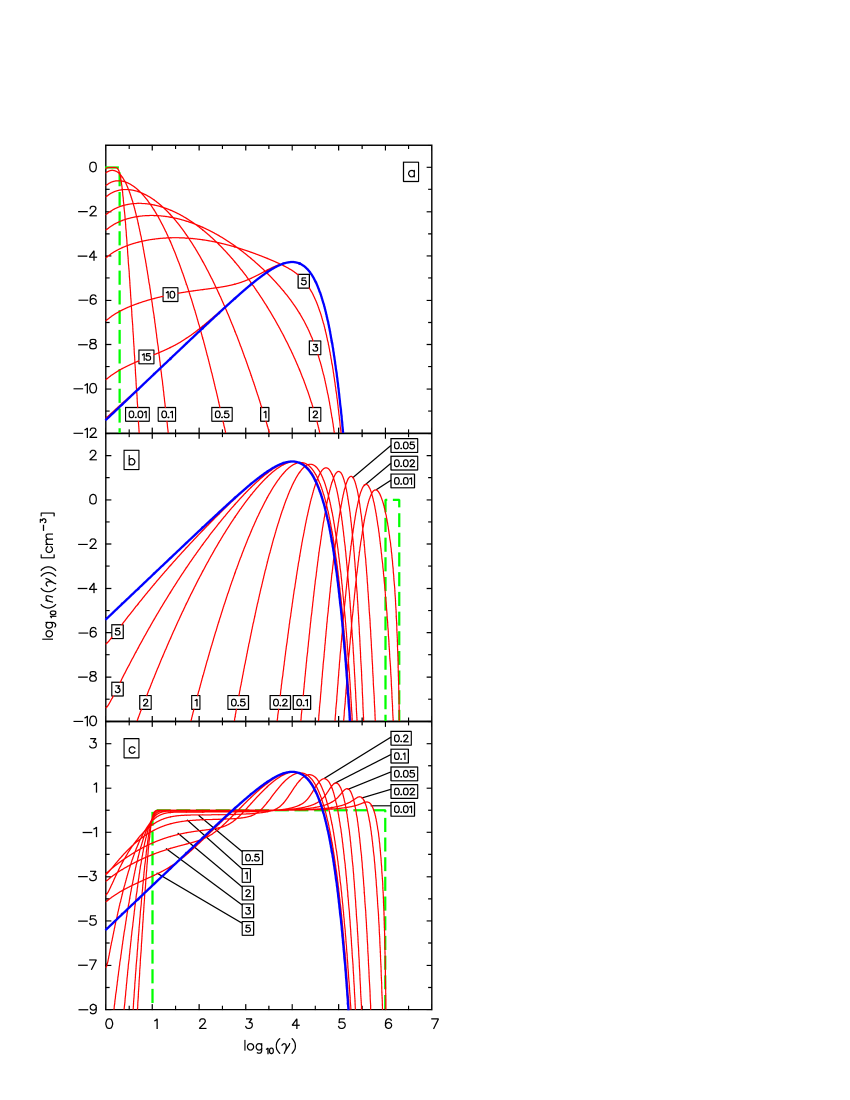
Figure 1: An example of the evolution of the electron spectrum in the case of no injection and escape of the particles. The upper panel (a) shows the evolution of the initial spectrum (bold dashed line) where the particle energy ($1\leq\gamma\leq 2$) is significantly lower than the equilibrium energy ($\gamma_{\rm e}=10^{4}$). The opposite case, where the initial energy ($10^{6}\leq\gamma\leq 2\times 10^{6}$) is higher than the equilibrium energy, is presented in the middle panel (b). The lower panel (c) shows a case where the lower energy in the initial spectrum is lower than $\gamma_{\rm e}$, but the upper initial energy is higher than the equilibrium energy ($10\leq\gamma\leq 10^{6}$). The stationary Maxwellian spectrum on all figures is indicated by a bold solid line. The numbers indicate the evolution time in units of $t_{\rm acc}$.

5.1 No injection and escape

In the first three tests we neglected injection and escape of the particles during the evolution of the system, and we analysed only the evolution of the initial spectrum.

• First, we assume a very narrow initial distribution ($1\leq\gamma\leq 2$) with an average energy of the particles significantly less than the equilibrium energy. The density of the particles is constant over the whole energy range of the initial spectrum. In this particular case $t_{\rm acc}\ll t_{\rm cool}$ for the initial energy of the particles. Therefore, the acceleration process tries to increase the energy of all the particles. In the case of the stochastic acceleration, some of the particles may reach the equilibrium energy or even a higher energy after an infinitesimally short time of the system evolution ($t_{0}+\Delta t$). However, the number of the particles that can gain this energy is negligibly small in comparison to the initial number of particles. The system needs more time to accumulate a significant number of the particles around the equilibrium energy. The simulation presented in Fig. 1a shows a systematic decrease in the particle density for the initial energy range and a simultaneous increase in the density around the equilibrium energy. In this particular case the densities in these two energy ranges become comparable after the evolution time of $t_{\rm evo}\gtrsim 5t_{\rm acc}$. After a longer time ($t_{\rm evo}\gtrsim 20\leavevmode\nobreak\ t_{\rm acc}$), the acceleration will significantly decrease the density of the particles with the initial energy, accumulating a dominant part of the particles around the equilibrium energy and reaching the stationary Maxwellian distribution. In the stationary state all of the energy acquired by the particles in the acceleration process is radiated away. Note that the deterministic acceleration in this particular test could shift the initial spectrum towards the equilibrium energy without significantly modifying the shape as long as the average energy of the particles in the system is significantly less than $\gamma_{\rm e}$. Close to the equilibrium any initial spectrum should be transformed by the deterministic acceleration into a quasi–monoenergetic distribution. Finally, the deterministic acceleration appears less efficient than the stochastic acceleration. For the same value of the acceleration time, this process requires at least twice as much time to build a particle density that is comparable to the density provided by the stochastic acceleration around the equilibrium energy.

• In the second test (Fig. 1b) we again assume a very narrow initial distribution, but now the average energy of the particles is significantly higher ($10^{6}\leq\gamma\leq 2\times 10^{6}$) than the equilibrium energy. At the beginning the cooling process dominates the evolution of the particle spectrum ($t_{\rm cool}\ll t_{\rm acc}$). Therefore the initial distribution moves towards the equilibrium energy. Note that in the case of a deterministic acceleration this particular initial spectrum could be transformed into a quasi–monoenergetic distribution. This is related to the fact that the cooling time is shorter for the particles with the highest energy. In our test, instead of the monoenergetic distribution, we obtain a kind of peaked spectrum that is more extended in the energy range than the initial spectrum. However, the peak energy of this distribution evolves in the same way as the energy of the monoenergetic distribution in the case of no diffusion. When the peak energy reaches $\gamma_{\rm e}$, the shift in the peak ceases because the cooling process becomes fully compensated for by the acceleration. On the other hand, after this moment in the evolution, the left part of the peaked distribution starts to change slope from an exponential to a power law. When the index of this power law becomes equal to 2, this evolution stops and the formation of the stationary Maxwellian distribution is completed.

• In the next test (Fig. 1c), the assumed initial spectrum is relatively broad ($10\leq\gamma\leq 10^{6}$). The initial minimal energy of the particles is significantly less than the equilibrium energy, but the maximal energy is significantly higher than $\gamma_{\rm e}$. For the sake of simplicity we also assume a constant particle density in this energy range. The specific assumption about the initial spectrum makes this case more complex than the previous ones. However, the evolution in this case in some specific energy ranges is very similar to the cases just discussed above. The change in the distribution before the minimal initial energy is similar to the evolution presented in our second test below the peak energy. Above the minimal energy, but below the equilibrium, the changes in the spectrum are similar to the evolution presented in our first test. Finally, above $\gamma_{\rm e}$ the evolution is analogous to the variations presented in our second test, above the equilibrium.

The tests described above show that indeed the stationary state is almost independent of the initial distribution in the absence of the injection and escape of the particles. Note that a constant escape of the particles ($E(\gamma,t)=N(\gamma,t))/t_{\rm esc}$) could produce a systematic decrease in the particle density proportional to a factor $\exp(-t/t_{\rm esc})$ without modifying the spectral shape (e.g. Schlickeiser (Schlickeiser84 (1984)). However, the escape and a simultaneous continuous injection are able to completely change the evolution and the resulting stationary spectrum. We discuss such scenarios in the next subsection.

5.2 Continuous injection and escape

In the next step we discuss three more cases where we assume continuous injection and escape of the particles. The escape in our calculations may be explained in two different ways. First, this term may describe a real escape of the particles into the region of a source where the magnetic field strength is significantly smaller and therefore the efficiency of the particle emission is also significantly less. The escape may also approximate adiabatic losses in the particle energy. The description of the adiabatic cooling inside an expanding source is slightly different from the description of the escape. However, the precise description of the SSC emission of an expanding source is beyond the scope of this paper.

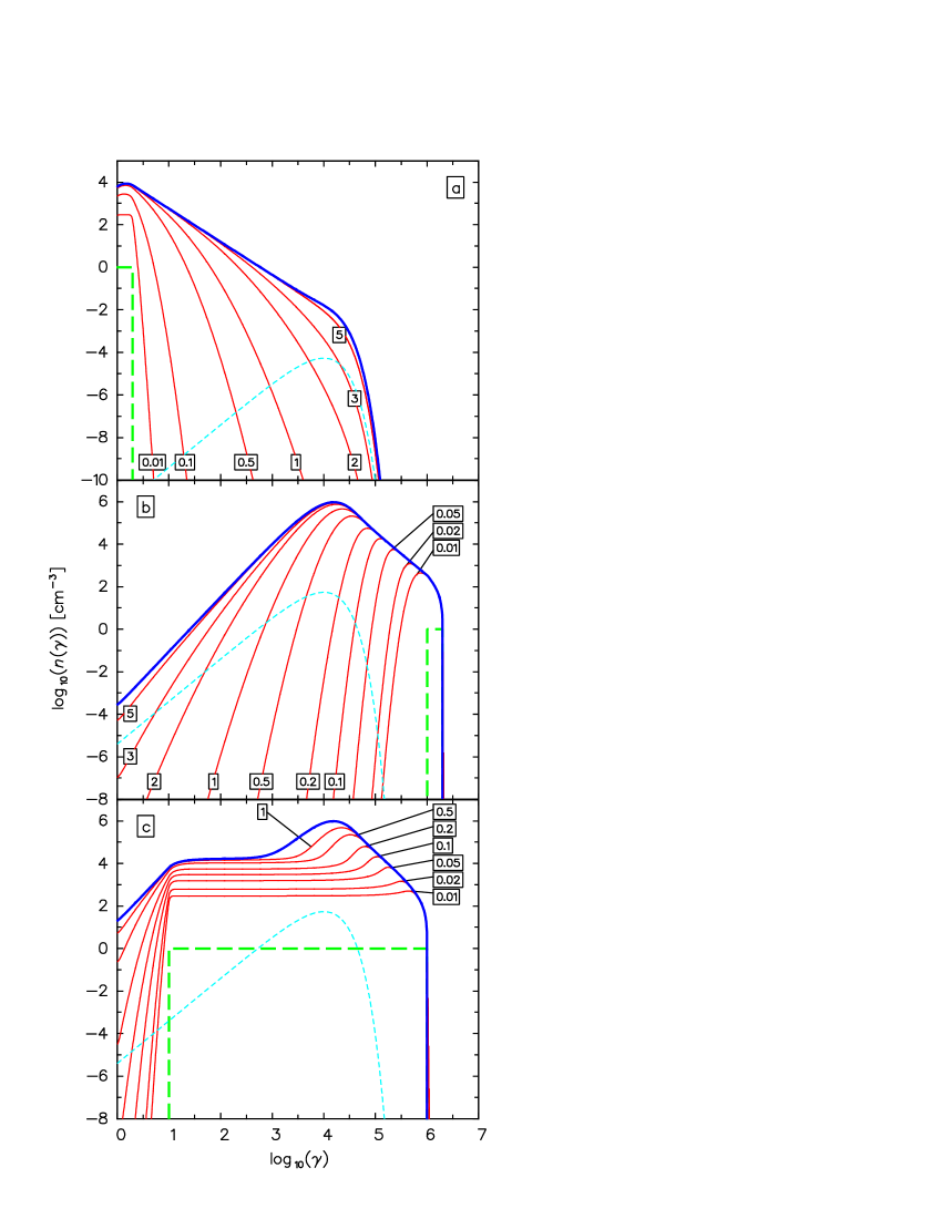
Figure 2: An example of the evolution of the electron spectrum in the case of continuous injection and escape of the particles. The bold dashed line shows the initial spectrum and the profile of the injection. We use the same parameters for the initial spectrum and the injection as in the simulations presented in Fig. 1. For a comparison, the stationary Maxwellian distributions obtained in the previous tests are presented by a thin dashed line.

In three more tests presented in this subsection we assume that the profiles of the continuous injection are equivalent to the initial distributions used in the previous tests:

• The injection profile in our fourth test is identical to the initial distribution in the first test (Fig. 2a). The particles are continuously injected at the lower energy ($1\leq\gamma\leq 2$) and systematically accelerated up to the equilibrium energy. The escape of the particles is described by the characteristic escaping time $t_{\rm esc}=t_{\rm acc}$. The competition between the acceleration and the escape in the case of continuous injection produces a power law distribution that extends from the maximal energy of the injected particles up to $\gamma_{\rm e}$. Below the maximal injected energy the spectrum is almost flat. Above the equilibrium energy the diffusion process produces an exponential cut–off. This makes this distribution different from the spectrum that could be produced in this case by the deterministic acceleration, where a pile-up or a roll-over is produced before the equilibrium energy, depending on whether the particle slope is softer or harder than 2. Moreover, the slope of the spectrum produced by the stochastic acceleration

  $$n\simeq 1+\frac{t_{\rm acc}}{2t_{\rm esc}}$$ (19)

  differs from the slope that could be obtained from the deterministic acceleration

  $$n=1+\frac{t_{\rm acc}}{t_{\rm esc}}$$ (20)

  (e.g. Kirk et al. Kirk98 (1998)). Note that basic shock–acceleration models postulate that $t_{\rm acc}\simeq t_{\rm esc}$, or in more sophisticated cases, postulate that $t_{\rm acc}$ and $t_{\rm esc}$ have the same energy dependence. Therefore the index of the particle energy spectrum predicted by such models should be $n\simeq 2$. In our acceleration scenario the value of the characteristic acceleration time is a free parameter, and the resulting index depends on the initial assumption. Moreover, $t_{\rm acc}$ and $t_{\rm esc}$ may have a different energy dependence in a more complex scenario. This may give much more complex spectra. However, as long as the energy dependence of the characteristic acceleration and escape time is defined by a power–law function, the resulting energy spectrum should also be a power–law function.

• The continuous injection above the equilibrium energy produces a power law spectrum up to the equilibrium. The evolution in this energy range is dominated by the cooling and escape process and therefore the index of the produced power law is equal to –2. Below the peak energy, the spectrum is systematically changed from an exponential to a power law at the stationary state. This change is similar to the evolution presented in our second test. However, the index of the resulting power law

  $$n\simeq-2-\frac{t_{\rm acc}}{2t_{\rm esc}},$$ (21)

  this time is steeper than the $\gamma^{2}$ slope necessary to obtain the Maxwellian spectrum in the second test.

• In the last test the particles are injected below and above the equilibrium energy (Fig. 2c). The evolution below the minimal injected energy is analogous to the evolution in the previous test below $\gamma_{\rm e}$. Above the minimal energy, the process is dominated by the injection and by the escape that leads to a flat stationary spectrum. Above the equilibrium energy the evolution is almost the same as in the previous test.

The simulations presented in this section show that the injection and escape may dominate the evolution of the spectrum and may lead to completely different stationary states. Note that in some of our simulations we assume for the sake of simplicity a very low energy of the initial or injected particles ($1\leq\gamma\leq 2$). However, the turbulent acceleration of such low energetic leptons may be difficult in an electron–proton plasma where thermal protons very efficiently damps resonant Alfvèn waves with the frequency equal to their gyrofrequency. Also a shock wave may have difficulty with the acceleration of such low energetic leptons. Only the particles with a Larmor radius larger than the thickness of the shock are able to ‘feel’ the shock discontinuity. Therefore, some pre–acceleration of the particles is required in order to let the turbulent or shock acceleration operate efficiently. Such pre–acceleration in our test could be simply taken into account by assuming higher energy for the initial or injected particles (e.g. $10\leq\gamma\leq 20$). Such a relatively small energy increase has a negligible impact on the evolution of the particle spectrum at very high energies ($\gamma\simeq 10^{6}$). Therefore, for the sake of simplicity we neglect the problem of the pre–acceleration in the tests, where we assume a relatively low energy for the initial or injected particles.

6 Evolution of the SSC emission

The evolution of the synchrotron emission depends directly on the evolution of the electron spectrum that also controls the inverse–Compton scattering process. We analyse here the SSC emission generated by a homogeneous, spherical source filled by electrons and a uniform magnetic field. The particles are accelerated uniformly throughout the emitting region. Out of the 6 evolutionary scenarios described in the previous section we, only investigate here two possible evolutions where the initial energy of the particles is relatively low ($1\leq\gamma\leq 2$). Using this simple model we try to explain the high–energy activity of Mrk 501.

6.1 No injection and escape

In the first test we assume no injection and escape of the particles from the acceleration region. This simulation is very similar to the first evolutionary scenario discussed in Sect. 5.

The main difference between the present simulation and the previous one appears in the particle cooling conditions. In the previous test we assumed, for the sake of simplicity, a constant cooling ($C=C_{0}\gamma^{2}$), which can be interpreted as the synchrotron emission in a constant magnetic field ($U_{B}\gg U_{\rm rad}$). Here, since we apply our results directly to the emission of the TeV blazar Mrk 501, we cannot neglect the radiative cooling due to the IC scattering. Moreover, we have to take the decrease of the scattering efficiency in the Klein–Nishina regime into account. This effect is approximated in our calculations by a constraint on the radiation–field energy density used for the computation of the cooling

$$U_{\rm rad}(\gamma,t)\simeq\frac{4\pi}{c}\int_{\nu_{\rm min}}^{\nu_{\rm x}(\gamma)}I_{\rm syn}(\nu,t)d\nu,$$ (22)

where $I_{\rm syn}$ is the intensity of the synchrotron emission, $\nu_{\rm x}(\gamma)=\min[\nu_{\rm max},3m_{e}c^{2}/(4h\gamma)]$, and $\nu_{\rm min}$, $\nu_{\rm max}$ are the minimal and maximal frequencies of the synchrotron emission, respectively. According to this formula for the very high energetic particles ($\gamma\gtrsim 10^{6}$), we have $U_{\rm rad}\lesssim U_{\rm B}$ in this particular test. On the other hand, the radiation field energy density is much larger than $U_{\rm B}$ for the low energy particles ($\gamma\lesssim 10^{2}$). This, as pointed out by Dermer & Atoyan Dermer2002 (2002), provides a quite complex form of the cooling term, which introduces a significant difference in the evolution of the electron spectrum (see also Moderski et al. Moderski05 (2005)). This difference is very visible if we compare the stationary state in the previous test (Fig. 1a) and the stationary spectrum in the present simulation (Fig. 3a). Previously we obtained a pure, Maxwellian distribution whereas now we have two bumps in the spectrum. The high–energy bump, that dominates the spectrum appears at the equilibrium energy related mostly to the acceleration process and the synchrotron cooling. The bump that appears at the lower energies is controlled by the acceleration and the IC cooling that is very strong only for the low energy particles. However, as long as the amplitude of the low energy bump is smaller than the amplitude of the high energy bump, the existence of the low energy bump is not visible in the synchrotron spectrum (Fig. 3b). The simple formula ($\alpha=(n-1)/2$) that describes the relation between the electron spectral index ($n$) and the index of the synchrotron emission ($\alpha$) becomes invalid when $n<1/3$. In such a case the spectral index of the power law part of the synchrotron emission becomes constant and $\alpha=-1/3$. This value is equivalent to the spectral index of the synchrotron emissivity of a monoenergetic population of the electrons, since in this case the electrons belonging to the high energy bump dominate the total synchrotron emissivity.

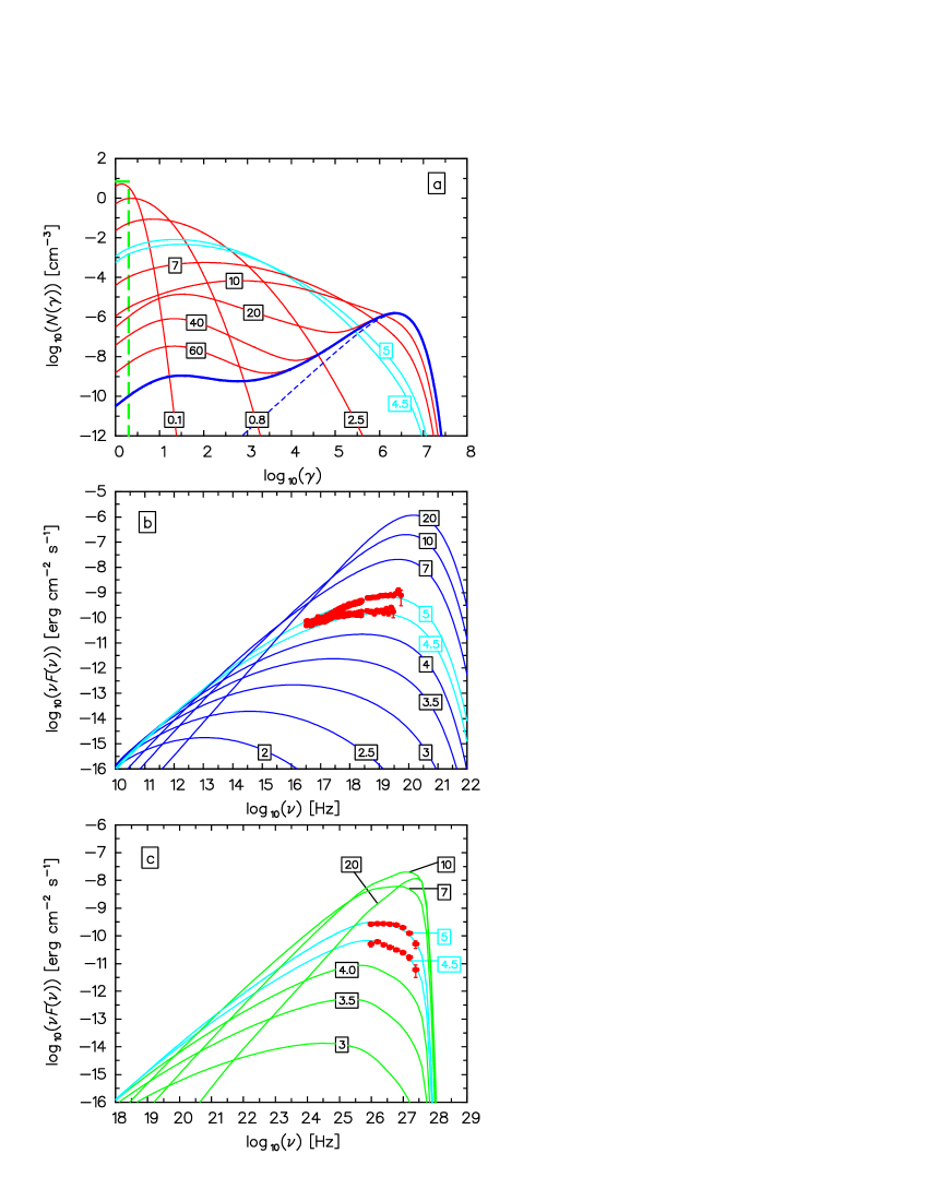
Figure 3: The upper panel (a) shows the evolution of the electron spectrum inside a homogeneous, spherical source in the case of no injection and escape of the particles. The remaining panels show the synchrotron (b) and the inverse Compton (c) radiation of the source. In this particular test we applied our model to the high energy emission of Mrk 501 observed almost simultaneously by the $Beppo$SAX (panel-b, Pian et al. Pian98 (1998)) and CAT (panel-c, Djannati–Atai et al. Djannati99 (1999)) experiments in April 1997. The lower level of the emission (7^th of April) is reproduced well by the source emission at the evolution time equal to 4.5 $t_{\rm acc}$ while the highest level (16^th of April) appears to be reproduced well by the emission at the time equal to 5 $t_{\rm acc}$.

The evolution of the synchrotron radiation presented in Fig. 3b shows that the $\nu F(\nu)$ peak of the emission is systematically increasing the amplitude and moving towards higher frequencies. However, the movement towards higher frequencies slows down significantly when the maximal particle energy becomes comparable with the equilibrium energy. On the other hand, the amplitude increases even if the peak frequency appears almost constant. The spectral index below the peak frequency changes simultaneously with the increase in the peak amplitude. However, as discussed above, the limiting value for the index is $\alpha=-1/3$, and this slope remains constant even if the peak amplitude is still increasing.

The changes in the IC emission, presented in Fig. 3c, are very similar to the evolution of the synchrotron radiation. However, the evolution of the peak position appears not to be as strong as in the case of the synchrotron emission. This is related mostly to the fact that the IC scattering is limited by the Klein–Nishina effect. Moreover, the very high energy gamma rays ($E\gtrsim 1{\rm TeV}$) are significantly absorbed due to interaction with the intergalactic infrared radiation field. Since we want to apply this simulation to the specific case of Mrk 501, the spectra shown take into account the absorption suffered by TeV photons interacting with the cosmic infrared radiation background, and therefore these cases assume a distance between us and the source that is equal to the distance of Mrk 501. The absorption produces a cut–off in the spectra above the frequency $\sim 10^{28}$ [Hz] in this particular case. To the calculate the absorption, we use the absorption coefficient derived by Kneiske et al. (Kneiske02 (2002), Kneiske04 (2004)). The spectral index of the IC emission below the peak is also limited by the value $\alpha=-1/3$.

As mentioned above, in order to check whether the discussed scenario is able to explain the high energy emission of TeV blazars, we apply the results of the simulation to the well–known high energy activity of Mrk 501 observed by $Beppo$SAX (Pian et al. Pian98 (1998)) and CAT (Djannati–Atai et al. Djannati99 (1999)) in April 1997. What is important for these data is that the X–ray/TeV observations were made almost simultaneously. However, we have to point out that there is a delay of a few days between the higher (16^th of April) and the lower (7^th of April) emission levels and these two emission levels were observed during different flaring events (Catanese et al. Catanese97 (1997)). Moreover, the X–ray (as well as TeV) spectra were gathered during a few hours of integration. The observed variability time scales of TeV blazars at X–ray/TeV energies are usually very short, from several minutes up to a few hours.

Our main aim was to show that our proposed model is able to reproduce such very short variability time scales with reasonable assumptions about the physical parameters. We apply our instantaneous spectra for the observations integrated over some period of time to roughly constrain the physical parameters. The presented data are one of the best quasi–simultaneous observational set ever obtained for TeV blazars. We used the same evolutionary scenario to explain both presented emission levels. This means that we use exactly the same values for the physical parameters in both cases. As shown in Fig. 3b/c, our modeling reproduces the observed spectra well if we select the radiation generated at the evolution time $t_{\rm evo}=4.5t_{\rm acc}$ for the lower emission level and $t_{\rm evo}=5t_{\rm acc}$ for the higher level. The characteristic acceleration time assumed in the calculations is equal to $R/c$, where $R=3.2\times 10^{15}$ [cm] is the source radius. We used also the Doppler factor $\delta=21$, an initial particle density $K_{\rm ini}=7$ [cm^-3], and the constant magnetic field intensity $B=0.05$ [G].

6.2 Continuous injection and escape

The second test presented in this section assumes continuous injection and the escape of the particles. As already shown (Fig. 2a), this scenario leads to a stationary solution that has a power law shape.

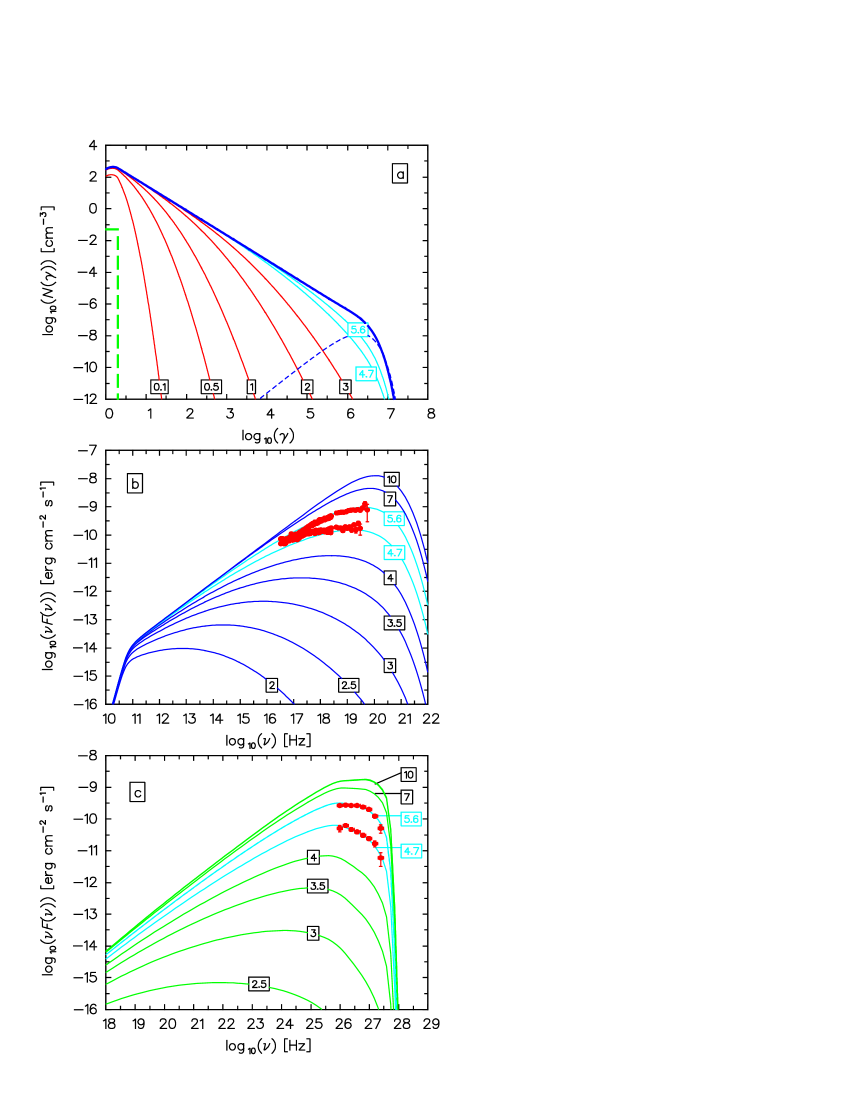
Figure 4: The evolution of the electron spectrum (a) and the SSC emission (b, c) in the case of continuous injection and escape of the particles. We apply this modeling again for the high energy activity of Mrk 501 observed in April 1997 (Pian et al. Pian98 (1998), Djannati–Atai et al. Djannati99 (1999)).

The cooling conditions in the present simulation are similar to the conditions described in the previous subsection. However, the complexity of the cooling in the Klein–Nishina regime now has no impact on the evolution of the low energy part of the spectrum. In the low energy range, the evolution of the spectrum is dominated by the acceleration and escape processes.

In the present simulation, the evolution of the peak position is very similar to the evolution in the previous test (Fig. 4b). The value of the spectral index below the peak also changes fast with the increase in the peak amplitude. However, now the limiting spectral index $\alpha\simeq 0.25$ is related to the assumption $t_{\rm acc}=t_{\rm esc}=R/c$ made in this particular test. The assumption, according to Eq. 19, gives the spectral index of the energy spectrum $n\simeq 1.5$ and the above–mentioned index of the synchrotron emission.

If we compare the IC emission in the previous test (Fig. 3c) with the same radiation in the present calculations, we see that the evolution in both cases is very similar. The scattering in the Klein–Nishina regime and the absorption of the TeV emission limit the evolution of the peak. The difference between the two simulations appears in the slope of the IC spectrum below the peak that now is $n\simeq 0.25$. The emission level at the end of the simulation (stationary particle distribution) in the present (as well as in the previous) simulation is much higher than the maximal observed level. However, the spectra selected from the evolution sequence before the stationary state provide a much better explanation for the observations than the spectra that correspond to the stationary state. Moreover, the variability of the TeV sources, where a fast increase in the observed flux is followed by an almost equally fast decrease (quasi–symmetric flare profile), may indicate that the source is almost never able to reach the stationary state. Therefore, a significantly higher level of the emission related to the stationary particle distribution is rather unlikely. Note also that relatively small modification in the high energy “tail” of the particle distribution produces very strong changes in the emission level.

To check the validity of the present simulation we again apply our results to the high energy activity of Mrk 501 observed in April 1997. We can reproduce the observed spectra well assuming $t_{\rm evo}=4.7t_{\rm acc}$ for the lower emission level and $t_{\rm evo}=5.6t_{\rm acc}$ for the higher level. This may suggest that in comparison to the previous test, the system needs twice as much time to evolve from the lower to the higher emission level. However, the source radius assumed in the preset test ($R=10^{15}$ cm) is more that three times smaller than the radius in the previous simulation ($R=3.2\times 10^{15}$ cm). This means that the discussed time was even shorter than in the previous case. We use the following values of the other model parameters: $\delta=33$, $B=0.11$ [G], and the the injected particles distribution $Q_{\rm inj}=5\times 10^{-2}$ [cm^-3 s^-1]. The parameters used in this test are quite similar to the parameters used in the previous calculations. The specific assumptions about some of the parameters and the number of free parameters required by the model are discussed in the next section.

7 Number of free parameters

In order to explain the SSC emission of a homogeneous spherical source filled by a uniform magnetic field and monoenergetic population of the electrons, we have to specify the size of the source ($R$), the magnetic field intensity ($B$), the particle density ($K_{\gamma}$), the energy ($\gamma$) of the particles, and the Doppler factor ($\delta$) if the source velocity is relativistic. This gives only five free parameters. However a monoenergetic population of the particles generates a synchrotron spectrum with the index $\alpha=-1/3$ and the exponential cut–off that do not provide a good fit to the observed spectra of TeV blazars.

Assuming a power–law distribution of the particle energy, we have to specify the density ($K_{\rm min}$) of the particles with the minimum energy ($\gamma_{\rm min}\simeq 1$) instead of $K_{\gamma}$ and the maximal particle energy ($\gamma_{\rm max}$) instead of $\gamma$. Moreover, we also have to specify the slope ($n$) of the electron distribution. This gives one more free parameter in comparison to the first model. The power–law distribution can explain some of the observations, but to explain most of the data we have to apply a more complex distribution.

Using a broken power–law energy distribution, we can explain most of the observed spectral shapes. However, to describe the broken power–law, we have to specify two more free parameters. This approach requires additional information about the break energy ($\gamma_{\rm brk}$) and the slope ($n_{2}$) of the second part of the energy spectrum. Therefore the model requires eight free parameters. It should be mentioned that in some cases when the second part of the electron spectrum is relatively steep ($n_{2}\gg 3$), the synchrotron and IC peaks are related to the break in the energy spectrum. Therefore $\gamma_{\rm max}$ is unimportant, which reduces the number of free parameters to seven. However, this simplification does not apply to the high–energy observations of Mrk 501 used in this work. To explain the data with the broken power law and the simple homogeneous model we have to specify at least eight free parameters (e.g. Katarzynski et al. Katarzynski01 (2001))

The model presented in this work uses a more complex spectra than either a power or a broken power–law. Our spectra are calculated self–consistently according to the assumed physical conditions. Therefore, instead of the spectral parameters, we have to describe the processes that control the evolution of the spectrum (acceleration, radiative cooling, initial spectrum, or continuous injection and possible escape). In principle, the model requires seven free parameters ($\delta$, $R$, $B$, $K_{\rm ini}$ or $Q_{\rm inj}$, $t_{\rm acc}$, $t_{\rm esc}$, and $t_{\rm evo}$). However, if we assume that the escaping process is negligible, then the number of free parameters is reduced to six. We made such an assumption in the first simulation that has been applied to the activity of Mrk 501 (Sec. 6.1). Moreover, we assume in this particular test that the acceleration time is equal to the light crossing time of the source ($R/c$), which reduces the free parameters to five. This is a completely arbitrary assumption, but it provides reasonable results. To explain the lower of the two observed emission levels, the source requires an evolution time equal to 4.5 $R/c$, in the first simulation. This gives about 6.5 hours in the observer’s frame. However, to get from the lower emission level to the higher level, the source requires only 0.5 $R/c$, which gives 0.7 h in the observer’s frame. This time scales are in good agreement with the variability time scales observed in TeV blazars (Maraschi et al. Maraschi99 (1999), Fossati et al. Fossati00 (2000), Aharonian et al. Aharonian02 (2002)).

In the second test performed to explain the activity of Mrk 501, we assumed continuous injection and escape of the particles. The characteristic escape time was assumed to be equal to the crossing time. This assumption describes on average the fastest possible escape of the particles. Moreover, we assumed that $t_{\rm acc}$ is also equal to $R/c$ as in the previous test. In fact the acceleration time cannot be longer than $R/c$ because the particles could escape from the source without a significant energy gain. On the other hand, the acceleration time can be shorter than $R/c$, which could correspond to a more efficient acceleration. However, $t_{\rm acc}\ll t_{\rm esc}$ do not provide the required slope of the electron spectrum ($n\eqsim 1.5\dots 2\to\alpha\eqsim 0.25\dots 0.5$). Assuming $t_{\rm acc}=t_{\rm esc}=R/c$ we reduce the number of free parameters to five ($\delta$, $R$, $B$, $Q_{\rm inj}$, $t_{\rm evo}$). This gives a significant advantage in comparison to a simple homogeneous SSC model with the broken power law electron spectrum. Moreover, our model describes a time–dependent evolution of the source emission. This gives the possibility of eliminating one more free parameter. Suppose that we have observations of the source in a stationary state. Then the evolution time ($t_{\rm evo}$) can be eliminated. This reduces the number of free parameters to only four.

The reduction of the number of free parameters with respect to the commonly used SSC models may have very important implications. Suppose that we can describe the emission with only three free parameters. Then the values of these parameters could be directly derived from the relationship for the synchrotron peak frequency, the level of the synchrotron emission at the peak and the observed variability time scales. This means that we could predict the IC emission from the observed X–ray radiation and verify for example the absorption of the very high energy gamma–rays by the infrared intergalactic radiation field. However, we again have to stress that in constructing our model we have made a few completely arbitrary assumptions (e.g. $t_{\rm acc}=R/s$). These assumptions provide quite reasonable results but this is not a proof that our model correctly describes the source evolution. Our assumptions require independent observational confirmation. Our main aim was only to show how some of the free parameters could be eliminated from the model. If we neglect the arbitrary assumptions, our time–dependent model requires seven independent parameters. This is the number of free parameters also required by simple stationary SSC scenario.

8 Summary

We have proposed a simple time–dependent model for the SSC emission of a homogeneous source, which has direct application for the high energy emission of TeV blazars. The most important assumption in our modeling is that the acceleration of the particles has a stochastic nature. To explain such a case, we use the momentum diffusion equation that describes the evolution of the particles energy spectrum. For the sake of simplicity we have not described the possible acceleration processes in details but assumed only a constant average efficiency of the acceleration that is a free parameter in our model.

We first analysed the stationary analytic solution of the diffusion equation. We show that for constant cooling conditions and in the absence of particle injection or escape, the competition between the stochastic acceleration and the radiative cooling may lead to a thermal or quasi thermal distribution of the particles. This result is in a good agreement with the results of Schlickeiser (Schlickeiser84 (1984)).

In the next step we used numerical solutions of the diffusion equation to analyse the time–dependent evolution of the electron energy spectrum. In the case of no injection and escape of the particles, the resulting stationary spectrum is almost independent of the initial distribution. Then, assuming a continuous injection and simultaneous escape of the particles, we have showed that the stochastic acceleration may lead to different energy distributions that depend on the assumptions about the spectrum of the injected particles. In the most realistic case, when particles are injected at the lowest possible energies, the stochastic acceleration in competition with the escaping generates a power–law particle distribution.

Finally, we applied our model for the high energy activity of Mrk 501 observed in April 1997. We have used two opposite scenarios for the evolution of the electron spectrum. First we investigated the case where the escape and injection of the particles is neglected. In the second test we instead assumed continuous injection and escape. In both cases we have obtained satisfactory fits for the observed spectra. We have to point out that our model describes time–dependent evolution of the emission using the number of free parameters that is comparable to or even less than the number required by the very simple SSC scenario.

We point out that a general prediction of this model is that in the phase of ongoing preequilibrium stochastic acceleration of a population of low–energy electrons (see Fig. 3/4 a,b), the emissivity level of the peak of the synchrotron emission and the energy of the peak are correlated, a behaviour already observed a few times in blazars (e.g. Fossati et al. Fossati00 (2000), Tanihata et al. Tanihata04 (2004)). We are going to investigate this problem in detail in our further work. We will also investigate some specific relations between the X-ray and the TeV light curves that are predicted by the model.

Finally, a straightforward extension of our study is the application to the case of powerful blazars, in which the dominant role in the cooling of the high-energy electrons is played by the external radiation field of the host quasar. In these sources, as opposed to the case of TeV BL Lacs, the low-energy branch of the IC component is well known from X-ray observations, providing a supplementary constraint to the model.

- (1) Aharonian, F., A., et al. 2002, A&A, 393, 89
- (2) Bell, A. R, 1978, MNRAS, 182, 147
- (3) Blandford, R. D., & Ostriker, J. P., 1978, ApJ, 221, 29
- (4) Blandford, R. D., & Eichler, D., 1987, Phys. Rep., 154, 1
- (5) Borovsky, J. E., & Eilek, J. A., 1986, ApJ, 308, 929
- (6) Brunetti, G., 2004, Proceedings of the NATO Advanced Study Institute, Series II, mathematics, physics and chemistry, Vol. 135
- (7) Catanese, M., Bradbury, S. M., Breslin, A. C., et al., 1997, ApJ , 487, L143
- (8) Chang, J. S., & Cooper G., 1970, Computational Physics, 6, 1
- (9) Chiaberge, M., Ghisellini, G., 1999, MNRAS , 306, 551
- (10) Dermer, C. D., Miller, J. A., & Li, H., 1996, ApJ, 456, 106
- (11) Dermer, C. D., & Atoyan, A. M. 2002, ApJ, 568, L81
- (12) Djannati–Atai, A., Piron, F., Barrau, A., et al., 1999, AA, 350, 17
- (13) Drury, L., 1983, SSRv, 36, 57
- (14) Dung, R., & Petrosian, V., 1994, ApJ, 421, 550
- (15) Eilek, J. A., & Henriksen, R. N., 1984, ApJ, 277, 820
- (16) Fossati, G., Celotti, A., Chiaberge, M., et al., 2000, ApJ, 541, 166
- (17) Ghisellini, G., Celotti, A., Fossati, et al., 1998, MNRAS, 301, 451
- (18) Jones, F. C., & Ellison, D. C., 1991, Space Sci. Rev., 58, 259
- (19) Kataoka, J., Takahashi, T., Makino, et al. 2000, ApJ, 528, 243
- (20) Katarzyński, K., Sol, H., & Kus, A., 2001, AA, 367, 809
- (21) Kirk, J. G., Rieger, F. M., Mastichiadis, A., 1998, A&A, 333, 452
- (22) Kneiske, T. M., Mannheim, K., & Hartmann, D. H., 2002, A&A, 386, 1
- (23) Kneiske, T. M., Bretz, T., Mannheim, K., & Hartmann, D. H., 2004, A&A, 413, 807
- (24) Krawczynski, H., Sambruna, R., Kohnle, A., et al., 2001, ApJ , 559, 187
- (25) Longair, M., S., 1992, High Energy Astrophysic, Cambridge Univ. Press, Cambridge
- (26) Maraschi, L., Fossati, G., Tavecchio, F., et al., 1999, ApJ, 526, L81
- (27) Massaro. E., Perri, M., Giommi, P., & Nesci, R., 2004, A&A, 413, 489
- (28) Mastichiadis, A., & Kirk, J., 1997, A&A, 320, 19
- (29) Miller, J. A., & Roberts, D. A., 1995, ApJ, 452, 912
- (30) Moderski, R., Sikora, M., & Blazejowski, M., 2003, A&A, 406, 855
- (31) Moderski, R., Sikora, M., Coppi, P. & Aharonian, F. 2005, MNRAS, submitted (astro-ph/0504388)
- (32) Mücke, A., et. al. 2003, Astropart. Phys., 18, 593
- (33) Petrosian, V., & Liu, S., 2004, ApJ, 610, 550
- (34) Pian, E., Vacanti, G., Tagliaferri, G., et al., 1998, ApJ, 492, L17
- (35) Press, W. H., et al. 1989, Numerical Recipes in Fortran, Cambridge Univ. Press, Cambridge
- (36) Saugé, L., & Henri, G., 2004, ApJ, 616, 136
- (37) Schlickeiser, R., 1984, A&A, 143, 431
- (38) Schlickeiser, R., 1989, ApJ, 336, 243
- (39) Tanihata, C., Kataoka, J., Takahashi, T., et at., 2004, ApJ, 601, 759
- (40) Urry, C. M., & Padovani, P. 1995, PASP, 107, 803
- (41) Virtanen, J. J. P., & Vainio, R., 2005, ApJ, 621, 313