Probing the temporal variability of Cygnus X-1 into the soft state

Building on results from previous studies of Cygnus X-1, we analyze Rossi X-ray Timing Explorer (RXTE) data taken when the source was in the soft and transitional spectral states. We look at the power spectrum in the 0.01 – 50 Hz range, using a model consisting of a cut-off power-law and two Lorentzian components. We are able to constrain the relation between the characteristic frequencies of the Lorentzian components, and show that it is consistent with a power-law relation having the same index (1.2) as previously reported for the hard state, but shifted by a factor $\sim 2$. Furthermore, it is shown that the change in the frequency relation seen during the transitions can be explained by invoking a shift of one Lorentzian component to a higher harmonic, and we explore the possible support for this interpretation in the other component parameters. With the improved soft state results we study the evolution of the fractional variance for each temporal component. This approach indicates that the two Lorentzian components are connected to each other, and unrelated to the power-law component in the power spectrum, pointing to at least two separate emission components.

1 Introduction

Cygnus X-1 is one of the most studied X-ray sources, and is often quoted as the prototype black hole binary system. The source exhibits two main spectral states, commonly referred to as hard and soft, with a brief intermediate state during transitions (e.g., Zdziarski et al. 2002; Zdziarski & Gierliński 2004). Recently, a study of the broad-band spectra of Cyg X-1, mainly in the hard state, has been presented by Ibragimov et al. (2005), and a comprehensive study of all states of the source in the 3–200 keV range has been carried out by Wilms et al. (2006). Several models have been proposed to explain the observed states and transitions. The two main components of such models are usually a geometrically thin, optically thick accretion disk and a hot inner flow or corona. The models vary in the geometry and properties of mainly the corona/Comptonizing region (for a review on coronal models, especially in regard to timing characteristics, see Poutanen 2001). However, changes in the inner radius of the accretion disk are a common source of variability in many models (e.g., Poutanen et al. 1997; Esin et al. 1998; Churazov et al. 2001; Zdziarski et al. 2002).

The changes in spectral state are evident also in the power density spectrum (PDS). In the hard state the PDS is characterized by a flat-topped component up to $\sim 0.2$ Hz, where it breaks to a $f^{-1}$ slope that steepens at a few Hz (e.g., Belloni & Hasinger 1990; Nowak et al. 1999). In the soft state the PDS is dominated by a $f^{-1}$ component that steepens around 10 Hz (e.g., Cui et al. 1997a). The 1996 state transition also revealed an intermediate PDS, showing a $\sim f^{-1}$ slope at lower frequencies, a flatter component around $0.3-3$ Hz, and above that similar to the hard state PDS. In many observations there is evidence for a quasi-periodic oscillation (QPO) at a few Hz (Belloni et al. 1996; Cui et al. 1997b; Cui 1999).

Previous studies of the PDS of Cyg X-1 have shown correlations between different temporal features as well as between temporal and spectral components (e.g., Gilfanov et al. 1999). Correlations between features in the hard state PDS were first reported in Wijnands & van der Klis (1999). Nowak (2000) showed that the hard state PDS of Cyg X-1 could be well fit using Lorentzian components. This was expanded in a large scale study of the hard state PDS conducted by Pottschmidt et al. (2003), who also included some ‘failed state transition’ PDS. A systematic study of the PDS for all spectral states of Cyg X-1 was conducted by Axelsson et al. (2005, hereafter Paper I) using archival data from the Rossi X-Ray Timing Explorer (RXTE) satellite. Using a model consisting of a cut-off power-law and two Lorentzian profiles, we were able to fit the majority of PDS, and follow the components from hard state through the transitions and back. While the results showed that the Lorentzian components were present in a significant fraction of the soft state PDS, their behavior was not well constrained. In this paper we reanalyze the soft state data and expand it with observations from an additional soft state in May-August of 2003, recently made available. With the improved soft state results we are able to decompose the PDS and study the contribution from each component separately.

We begin this paper with a brief description of the data used, the analysis procedure and the model components (Sect. 2). This is followed by a presentation of our results in Sect. 3. In Sect. 4 we discuss our findings, and put them in context of other results. Finally our findings are summarized in Sect. 5.

2 Observations and Data Analysis

The data and methods of analysis used in this paper are in essence the same as in Paper I. Therefore we only give a brief summary of the data and extraction process, with emphasis on the new data and the parts of the analysis that have been improved. For more details we refer to Paper I.

2.1 The archival data

Since its launch on December 30, 1995, the RXTE satellite has observed Cyg X-1 in more than 750 pointed observations, with a typical on-source time of 3 – 4 ks. During this time, the All-Sky Monitor (ASM) instrument on board the satellite has also provided a continual coverage of the source in the 2–12 keV range.

As in our previous study, the data are obtained with the Proportional Counter Array (PCA, Jahoda et al. 1996) on RXTE, which consists of five identical Proportional Counter Units (PCUs), and is sensitive in the 2–60 keV energy range. The new soft state roughly spans the time from May 2003 to August 2003. We include all pointed observations made of the source during these four months, $\sim 4$ days per month. Note that some of these data are presented in Pottschmidt et al. (2005). The data mode used was the ‘Generic Binned’ mode. We also calculate count (hardness) ratios, using data from the Standard2 configuration.

Lightcurves were extracted with the standard RXTE data analysis software FTOOLS, version 5.2, using standard screening criteria: a source elevation $>10^{\circ}$, a pointing offset $<0\aas@@fstack{\circ}01$ and a South Atlantic Anomaly exclusion time of 30 minutes. The energy range of the data used for the PDS is $\sim 2-9$ keV, with the soft and hard bands of the count ratio taken as $2-4$ keV and $9-20$ keV respectively. For the PDS, the lightcurves were extracted with a time resolution of 10 ms. The lightcurves used in determining count ratios were extracted with 16 s time resolution. All lightcurves were normalized to one average PCU using the FTOOL correctlc.

2.2 Calculating the power spectra

The modelling of the soft state PDS in Paper I (e.g., Fig. 9) showed the need to extend the studied frequencies above 25 Hz. This requires proper treatment of dead-time effects, and we therefore correct the estimated Poisson level. We use the correction for general paralyzable dead-time of Zhang et al. (1995) as presented in the first corrective term in Eq. 6 of Jernigan et al. (2000). We chose an upper limit of 50 Hz.

To calculate the power density spectra the high-resolution light curves were divided into segments of $2^{13}$ bins ($\sim 82$ s). The resulting PDS were then gathered into groups of 10 and each group averaged into one final PDS. Each PDS thus covers $\sim 15$ minutes of observation time, allowing changes occuring on this timescale to be studied. As shown in Paper I, significant changes in the PDS of Cyg X-1 do occur on these short timescales. The PDS have been rebinned using semi-logarithmically spaced bins.

The normalization used for the PDS is that of Belloni & Hasinger (1990) and Miyamoto et al. (1992), where the integral over a frequency range gives the square of the fractional root-mean-square (RMS) of that frequency interval. In addition, the PDS are plotted in units of frequency times power versus frequency ($fP_{f}$ versus $f$). Together with the new data from 2003, the soft state data from Paper I were reanalyzed and corrected for dead-time effects, improving the signal-to-noise ratio. Altogether, a total of 614 soft state PDS were obtained.

2.3 Modeling

Nowak (2000) showed that the PDS of Cyg X-1 in the hard state could be successfully fit using Lorentzian components. The model was extended by Pottschmidt et al. (2003), who added a power-law component in order to fit the lower frequencies, especially during the ‘failed state transitions’. Building on these results, it was shown in Paper I that by introducing a cut-off power-law component together with two Lorentzians, we were able to provide a good fit to the PDS of Cyg X-1 in all states of the source. We could thereby for the first time model the complete evolution of the PDS. As the parameters of that model differ somewhat from those in the previous studies, we present their definition again here. The Lorentzian profiles have the form

$$L_{i}(f)=\frac{H_{i}W_{i}\nu_{i}}{(f-\nu_{i})^{2}+fW_{i}\nu_{i}}$$ (1)

where $H_{i}$ is the value of $fP_{f}$ at the peak frequency $\nu_{i}$. The dimensionless parameter $W_{i}$ gives a measure of the relative width of the profile in the $fP_{f}$ representation. The parameterization is chosen such that for a given $W_{i}$ and $H_{i}$, the integral of the Lorentzian (and thus its fractional contribution to the total RMS variability) is the same for any value of $\nu_{i}$. The cut-off power-law necessary in the transitional and soft states is of the form

$$Pl(f)=Af^{-\alpha}e^{-f/f_{c}}$$ (2)

Where A is the normalization constant, $\alpha$ is the slope, and $f_{c}$ is the turnover frequency. Of the 614 soft state PDS obtained from the observations, 143 allowed a fit using all three components of the model, one or both Lorentzian components being too weak to constrain in the remaining PDS. These fits were first performed with all parameters free, and then with the width of the first Lorentzian, $W_{1}$, frozen to a value of 0.6. While freezing $W_{1}$ did not affect the number of PDS where $L_{2}$ was detected, it allowed us to better constrain $L_{2}$ in those cases and the results of these latter fits were therefore kept. Table 1 lists the results of all fits used in this paper, including the ones from Paper I, and is available at the CDS in electronic form only. The first six columns give the proposal number and sub-ID (e.g., “60090-01-39-00”), the start and stop times in MJD of the lightcurve used to calculate the PDS, a number identifying the model components present in the fit, and the average 2–9 keV flux and (9–20 kev)/(2–4 keV) hardness during that time. This is followed by 18 columns giving the parameter value and error for the three parameters of the power-law ($A,\;\alpha,\;f_{c}$) and the parameters of each of the two Lorentzians $L_{1}$ and $L_{2}$ ($\nu_{i}$, $H_{i}$, and $W_{i}$).

The model used is not aimed at giving the fullest possible description of the PDS of Cyg X-1. For example, we do not attempt to model very small features of the PDS, and indeed the signal-to-noise ratio is insufficient for us to accurately do so. The strength of the model lies rather in its simplicity, allowing us to accurately fit the main characteristics of the PDS in all states, and track changes occuring on short timescales. Including a cut-off to the power-law proved essential in allowing the same model to fit all states, thereby giving a more complete picture of the power spectral evolution.

2.4 Definitions of state

When determining the state of Cyg X-1, it is possible to look at characteristics of either radiation spectra or temporal analysis. Current definitions of state, derived from either of these characteristics, are mainly phenomenological. These definitions all agree on the ‘classical’ hard and soft states. However, difficulties arise when attempting to define the extent of these states, and the boundaries of the transitional (or intermediate) state. Until the physical processes behind the state transitions are understood, these definitions will retain some of their arbitrary nature.

In an extensive study of the radiation spectra of Cyg X-1 in all states, Wilms et al. (2006) showed that there is a continuous spectral evolution between the states of the source. While timing spectra are generally able to provide sharper criteria, it was shown in Paper I that there is a continuum of PDS between the hard and soft states, with examples covering all stages of the evolution. Therefore, criteria of state such as the temporal features crossing certain frequency boundaries, or the appearance of a power-law component, do not by themselves provide good indicators of state. However, our previous study also revealed that several parameter correlations change behavior at the same stage of the evolution, and we therefore regard these changes to be a natural marker of the source entering the transitional state. Studies have also shown decreased coherence and enhanced time lags between the hard and soft lightcurves during transitions, both in Cyg X-1 (Cui et al. 1997b; Pottschmidt et al. 2000) and other sources (such as GX~339-4 and XTE~J1650-500, see Nowak et al. 2002; Kalemci et al. 2003, respectively). Benlloch et al. (2004) use a combination of photon index $\Gamma$ and time lags between the $2-4$ keV and $8-13$ keV channels to define the state of Cyg X-1. In their long term study of the hard state, Pottschmidt et al. (2003) showed that the state is not uniform, and a distinction is made between ‘quiet’ and ‘flaring’ hard states, where flares and ‘failed state transitions’ are more frequent in the latter. The classification of state is thus not rigorously defined, and remains an area of active research (for a recent review, see Zdziarski & Gierliński 2004).

For consistency with Paper I, we have used the same criteria when defining state, based on the changes seen in the temporal components. With this definition, the PDS in the hard state only show $L_{1}$ and $L_{2}$. As the source enters the transition, the power-law component enters the frequency window, and several parameter relations change behavior. In the soft state, $L_{2}$ is not seen or significantly weaker than $L_{1}$, or the PDS is completely dominated by the cut-off power-law component. For comparative purposes, we note that our definition is consistent with a criterion of the effective spectral index ($3-12$ keV) $\Gamma\ga 2.4$ for the soft state used elsewhere (e.g., Zdziarski et al. 2002).

During the ‘quiet’ hard state, there are periods when a third component appears at the higher frequencies of the PDS and the hardness increases. We refer to these episodes as the ‘hard edge of the hard state’, and while we do not model them in this paper, they are part of the data from Paper I presented in Sect. 3.3.

3 Results

We now turn to the results of our analysis, starting with the study of the soft state data. Following this analysis, we show that a decomposition of the PDS is now possible, and present the evolution of each temporal component.

3.1 The two Lorentzians

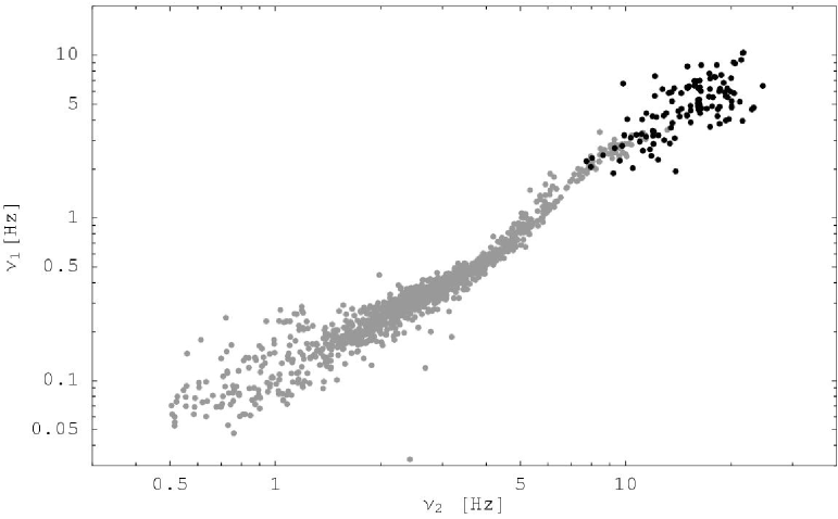
Figure 1: Relation between the two peak frequencies of the Lorentzian components. The grey points are 1414 hard state and transition points from Paper I, while the black points are 143 soft state points resulting from the analysis in this paper.

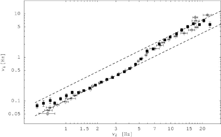
Figure 2: Results of binning in $\nu_{1}$ (open diamonds) and $\nu_{2}$ (solid squares). The lower line is the same as in Fig. 17 of Paper I, a fit to the hard state points (index $1.20\pm 0.01$), and the upper one a power-law with the same index ($1.19\pm 0.14$) fit to the soft state points (binning along $\nu_{2}$). Note how the binning along $\nu_{1}$ deteriorates as the source enters the soft state, but follows the power-law in the hard state to the lowest frequencies. The binning along $\nu_{2}$ deviates from the hard state fit at the lower frequencies, but extends the relation in the soft state to higher frequencies.

While the peak frequencies of the two Lorentzian components follow a power-law correlation in the hard state, the relation in the soft state is still uncertain ( Paper I, Fig. 9). As this deeper study is partly aimed at resolving this behavior, we begin by showing the frequency relation in Fig. 1. As can be seen in the figure, the spread of points is quite large in the soft state (black points). To determine whether there is a significant trend also in the soft state we will attempt to bin the data points. The problem with the binning is the same as in the more common case of regression, when choosing which parameter to treat as the independent one. In order to determine the effect of the binning procedure in this particular case we first performed Monte Carlo simulations, where we introduced noise to points following a power-law relation with known index. The resulting distributions were then binned along both axes and the indices determined. As long as the uncertainties are small, binning the data recovers the correct index. However, the results clearly show that an increase in noise tends to produce an artificial flattening effect along the axis of binning. If the amount of noise varies between the parameters, the best results are achieved when binning is done along the parameter with smallest errors. Returning to the analogy with regression, this amounts to the parameter with the smallest errors being chosen as the independent one. In addition, as our frequency range is limited, there are border effects as the components approach these limits, causing a biased distribution in the frequency nearest the border.

We now apply the same binning procedure to the data points of Fig. 1. In the soft state, the largest spread is along $\nu_{1}$. Therefore, binning along $\nu_{2}$ more accurately reveals the behavior of the relation. Conversely, for the hard state data, it is the spread along $\nu_{2}$ that dominates. In this range, binning along $\nu_{1}$ gives a better indication of the behavior of the relation. Figure 2 shows the result for both binnings. Also included in the figure is the power-law fit to the hard state points made in Paper I, with index $1.20\pm 0.01$, as well as a power-law fit instead to the points in the soft state (solid squares). Between the extremes, the results of the two binnings are indistinguishable. The flattening effects seen in Fig. 2 as the components approach the frequency limits are in agreement with the results of our simulations. Our change of binning parameter is thus well founded, but the outermost points at either extreme should be treated with caution.

With the better soft state data and the binning along $\nu_{2}$, it is clear from Fig. 2 that the relation in the soft state follows a power-law with an index similar to that of the hard state. The result is of course dependent on the where the soft state region is assumed to begin. Setting the lower limit too high in frequency ($\nu_{2}\ga 10$ Hz) results in a large uncertainty as the dispersion is high in this region. Lowering the boundary to include the asymptotic behavior of the transition ($\nu_{2}\ga 7$ Hz) reduces the fitting error, but introduces a systematic effect increasing the index. For all reasonable choices of this boundary (i.e., $7$ Hz $\la\nu_{2}\la 10$ Hz) an index of 1.2 is consistent with the result of the fit. We will assume a conservative estimate of $1.19\pm 0.14$ as the index for the soft state points, with the value derived from the fit with boundary at 8.8 Hz, and the error reflecting the variations arising from the range of possible boundary choices. The form of the power-law used for these fittings is:

$$\nu_{1}=B\;\nu_{2}^{\beta}$$ (3)

where $B$ is a constant and $\beta$ the power-law index.

Adopting the fits for the two states, a look at the constants of the power-laws reveals the values of $B=0.103\pm 0.002$ in the hard state and $B=0.19\pm 0.05$ in the soft state. The ratio of the constants is close to 2, and together with the fitted indices a shift of the hard state relation by a factor of two is consistent with the data. Is it therefore possible that the break in the relation during the transitions is simply a shift to a higher harmonic? In order to accurately model such a shift, three components would be necessary during the transitions. As our model only contains two components, it would not catch the change if the shift occurs gradually. Unfortunately, attempting to fit the PDS with three Lorentzian components shows that a third component is impossible to constrain in the data, and rarely produces a better fit. We therefore attempt a different approach using simulations.

3.2 Simulations

In order to test the hypothesis of $L_{1}$ shifting to its first harmonic, we conducted a series of Monte Carlo simulations where such an effect was included. Artificial power spectra were created and fitted with our model of two Lorentzian components plus a cut-off power-law. As input parameter for the simulations we use $\nu_{2}$, the peak frequency of $L_{2}$. This is to get the same distribution of frequency points as in the observed data. For the other parameters we utilize the parameter correlations found in Figs. 10-13 of  Paper I. We use analytic expressions to approximate these behaviors (shown in Fig. 3), adding some random Gaussian spread. For each $\nu_{2}$ a corresponding $\nu_{1}$ was derived assuming the hard state relation between the frequencies (lower line in Fig. 2), and values for $H_{2}$ and $W_{2}$ were calculated. Finally, a third Lorentzian component, $L_{1}^{+}$, was added with $\nu_{1}^{+}=2\nu_{1}$, i.e. the first harmonic of $L_{1}$. The parameters $W_{1}$, $W_{1}^{+}$, $H_{1}$ and $H_{1}^{+}$ were now determined from the relations seen in the left panels of Fig. 3. As $W_{1}$ is measured to center around one value at lower frequencies, and a lower value at higher frequencies, these different values were adopted for $W_{1}$ and $W_{1}^{+}$ (solid and dashed lines in panel b of Fig. 3 respectively). To simulate a shift in power from $L_{1}$ to $L_{1}^{+}$ during the transitions, the analytical approximation shown in panel a of Fig. 3 was multiplied by modulating factors:

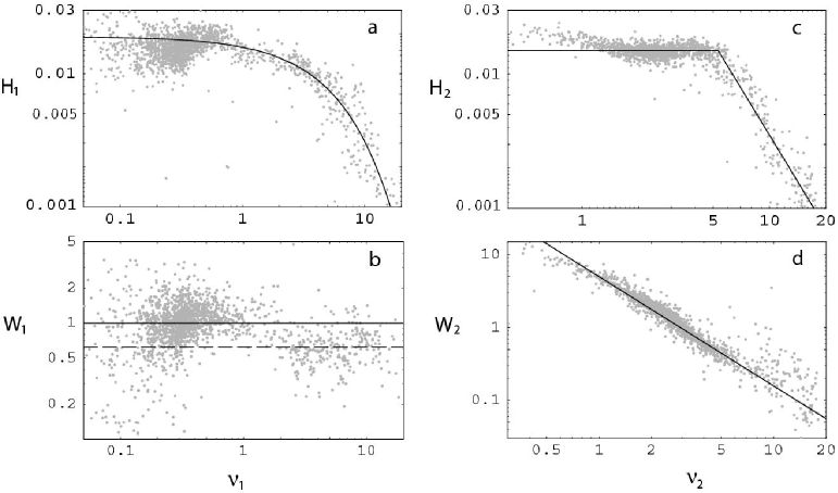
Figure 3: The parameter correlations from Paper I (gray points) and the analytical expressions used to approximate them in the simulations (black lines). The two left panels show $H_{1}$ (panel a) and $W_{1}$ (panel b) as a function of $\nu_{1}$. The two right-hand panels show the correlations for $H_{2}$ and $W_{2}$ versus $\nu_{2}$ (panels c and d). In panel b, the black line indicates the approximation used for $L_{1}$ and the dashed line for $L_{1}^{+}$. Note also the deviation from the approximation at the lowest frequencies in panel d. These points are from the hard state, when $L_{1}$ approaches the lower frequency boundary, and when the hardness is highest. As our simulations mainly cover the transition and soft state, this deviation does not influence our results.

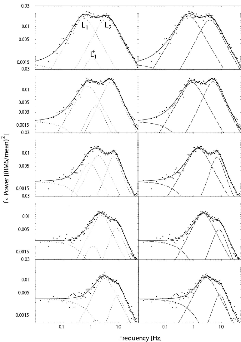
Figure 4: A sequence of five simulated power density spectra, displaying the evolution from hard state to the soft state (top to bottom). The panels on the left show the simulated model components (dotted lines): a lower frequency Lorentzian $L_{1}$ and its first harmonic $L_{1}^{+}$, a high frequency Lorentzian $L_{2}$ and a cut-off power-law. The solid line is the sum of the noise free components, the points indicate the result after the addition of noise. The panels on the right show the results of fitting the simulated PDS with our model, using only two Lorentzians and a cut-off power-law (dashed lines). The solid line is the sum of the components. Note that even when $L_{1}$ and $L_{1}^{+}$ are of nearly equal strength (e.g., third row from top), they are not resolved in the noise free PDS (solid line in left panel), and the sum is well fit by one wider Lorentzian component.

$$m_{1}(\nu_{2})=\frac{1}{1+\exp[-\frac{\nu_{t}-\nu_{2}}{\Delta\nu}]}\\ m_{1}^{+}(\nu_{2})=\frac{1}{1+\exp[+\frac{\nu_{t}-\nu_{2}}{\Delta\nu}]},$$ (4)

where $m_{1}(\nu_{2})$ is the factor for $H_{1}$, $m_{1}^{+}(\nu_{2})$ the factor for $H_{1}^{+}$, $\nu_{t}$ the value of $\nu_{2}$ roughly in the middle of the transition (6 Hz $\la\nu_{t}\la 7$ Hz) and $\Delta\nu$ is a constant related to the width of the transition ($\sim 1$ Hz). The values of these parameters are constrained by the transition region as seen in Fig. 2. The figure shows that the influence of $L_{1}^{+}$ must start at $\nu_{2}\sim 4$ Hz and completely dominates above $\nu_{2}\sim 8$ Hz. In our simulations, $\nu_{t}$ was set to 6.5 Hz and $\Delta\nu$ to 1 Hz.

Finally, a power-law component was added and random Gaussian noise was added to the resulting PDS to account for the uncertainty of the measured PSD values, and thereby giving the same signal-to-noise ratio as in the observational data. We use Gaussian noise as the PDS are the results of both averaging and rebinning, making the fluctuations approximately Gaussian. This assumption is least valid at lower frequencies, as each bin here is the average of only a few points. However, these frequencies are not of interest in this context. Examples of resulting PDS are shown in the left column of Fig. 4, along with the result of the fitting (right column). The difficulty of resolving the two components is very clear in the figure. As the width of each Lorentzian is very large compared to their separation, they are unresolved even in the pure signal (solid black line in the left-hand panels). Thus, even with a large increase in signal-to-noise ratio it will not be possible to determine directly whether these two components are in fact present in the data. This becomes more clear in Fig. 5, which shows the result of the fitting routine when $L_{1}$ and $L_{1}^{+}$ are equally strong, reflecting the most favorable scenario. From the residuals of the fit (bottom panel), it is clear that a single Lorentzian can successfully replace both $L_{1}$ and $L_{1}^{+}$.

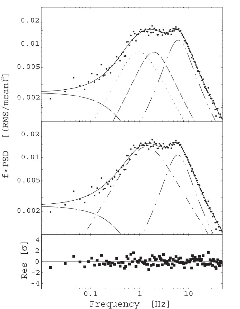
Figure 5: Result of fitting an artificially created PDS with the same model used for the data. The simulated PDS is shown in the top panel, with the power-law component as the long-dashed line, $L_{1}$ dotted, $L_{1}^{+}$ dashed and $L_{2}$ dot-dot-dashed. The middle panel shows the result of the fit using only two Lorentzian components, $L_{1}$ (dot-dash) and $L_{2}$ (dot-dot-dash). The bottom panel shows the residuals of the fit. Note that there is no trace of the third component. Trying to add a third Lorentzian to the fit is not feasible, as the data do not allow it to be constrained.

The artificial PDS were put through the same fitting routine as the observed data, and the parameters of the resulting fits (right-hand panels in Fig. 4) plotted in the same way. Fig. 6 shows the resulting frequency correlation. Fitting the artificial PDS with the model used for the data produces results nearly identical to those obtained from the observational data. Not only is the change in behavior around the transition ($\nu_{2}\sim 4-9$ Hz) the same, but when comparing with Fig. 1 it is apparent that also the general trend of the data points is reproduced. The relative dispersion is greater during the soft and hard states, with a minimum occuring during the transitions. As the components move to lower frequencies, the points in Figs. 1 and 6 both show the same gradual increase in relative dispersion. However, the dispersion of the soft state points is smaller in the simulations than in the data. This difference can be traced to the cut-off of the power-law component. As the power-law extends through most of the frequency range in the soft state, placing the cut-off too high in frequency will capture power from $L_{2}$. Since $L_{2}$ is weak in the soft state, this artificial weakening increases the uncertainty in frequency. In our simulations, we can use our knowledge of the power-law to eliminate this effect, thus reducing the dispersion in the soft state. When the parameters of the power-law are left completely free also in our simulations, the scatter of the soft state points is significantly increased.

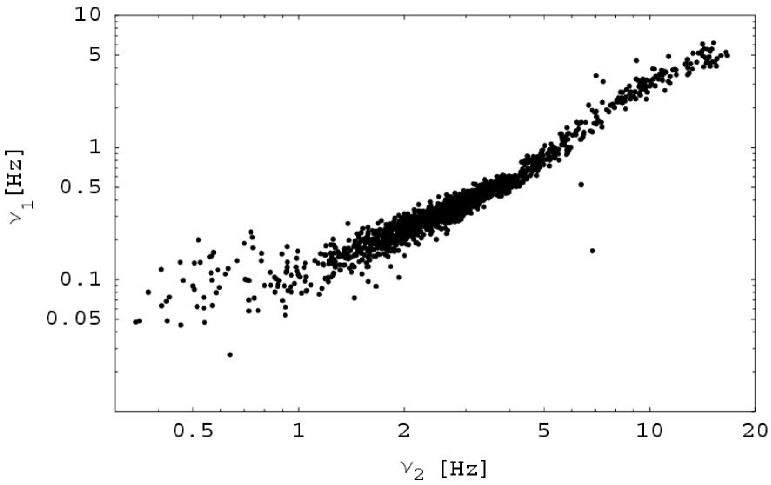
Figure 6: Results of fitting artificially created PDS with the same model used for the data. In the artificial PDS a shift from $L_{1}$ to its first harmonic is introduced, successfully reproducing the behavior in the data. Note that the general trends of Fig. 1 are also reproduced: increased relative spread towards the lowest frequencies, low relative dispersion during the transition and increased relative spread in the soft state.

It should be noted that the results do not change significantly if the amount of noise introduced is changed, nor does it depend to any large extent on the exact expression used to approximate the parameter relations. Perhaps not surprisingly, the results are most sensitive to the modulation function used to vary the strengths of $L_{1}$ and $L_{1}^{+}$. This is evident in the $H_{1}-\nu_{1}$ relation (panel a in Fig. 3). If $L_{1}$ starts to decline while $L_{1}^{+}$ is still very weak, the fitted $H_{1}$ values will show a dip at the corresponding frequency, and there is no such feature present in the data. We have tested expressions with both asymptotic exponential behavior and behavior of power-laws of varying index. The conclusion is that the rise of $L_{1}^{+}$ and the decay of $L_{1}$ must be fairly swift. This is also evident from the data in Fig. 1, as the transition occurs over a fairly narrow frequency range. We found that the observational results were most readily reproduced using exponential functions, as in Eq. 4. Using, e.g., polynomial modulation functions will achieve good agreement with the frequency relation of Fig. 1, but cannot successfully reproduce the other parameter relations (gray points in Fig. 3). In particular, the inadequacy in correctly reproducing the parameter correlations was seen also for modulations of the functional form $\left(1+\left(\nu/\nu_{0}\right)^{2}\right)^{-1/2}$, typically associated with band-pass filters.

The results from the simulation reproduce the behavior observed from the data for all parameter correlations. The interpretation of a shift in power from $L_{1}$ to its first harmonic during hard to soft transitions is therefore consistent with the data.

3.3 Evolution of the PDS

We now return to the observations, and with the improved results from the fits of the soft state, we attempt to separate the power spectral components and study their evolution through the spectral states. For this analysis we use both the data presented here, complemented with the data of Paper I. The goal should be to ultimately understand the relation between the components of the temporal variability and those of the radiation spectrum. The transitions are of key importance since they are associated with many changes in both timing and radiation properties. To measure the relative strength of each PDS component, and its evolution, we computed the fractional RMS by integrating over the $0.01-50$ Hz range. The result is shown in Fig. 7 together with the total fractional RMS, $\widetilde{\sigma}_{\rm tot}$, defined as

$$\widetilde{\sigma}_{\rm tot}\equiv\frac{\sigma_{\rm tot}}{F}\,,$$ (5)

where $\sigma_{\rm tot}$ is the total RMS and $F$ the mean flux of the lightcurve used in calculating the PDS. We furthermore assume that

$$\sigma^{2}_{\rm tot}=\sigma^{2}_{\rm lor}+\sigma^{2}_{\rm pl}\,,$$ (6)

where $\sigma_{\rm lor}$ and $\sigma_{\rm pl}$ correspond to the RMS of both Lorentzians and the power-law component respectively. It is assumed that both Lorentzians are produced by the same process, independent of that generating the power-law component. Since we neglect power below $0.01$ Hz, the RMS values for the power-law component should be seen as lower limits.

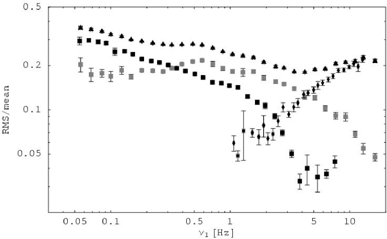
Figure 7: Total fractional RMS (triangles) in the 0.01-50 Hz range and contribution of each component, plotted against $\nu_{1}$. Black squares indicate the contribution from $L_{1}$ and $L_{1}^{+}$, grey squares from $L_{2}$ and diamonds from the power-law. Note how the total fractional RMS stays nearly constant throughout the hard state, dips during the transitions and increases again in the soft state. The increase below $\nu_{1}\sim 0.2$ Hz corresponds to the observations with highest hardness ratio, where a third Lorentzian component is seen to enter the PDS. These cases make up less than 10% of the total hard state observations.

Figure 7 shows that $\widetilde{\sigma}_{\rm tot}$ remains quite constant throughout the hard state ($\nu_{1}\la 0.65$ Hz). The exception to this is the range with the highest hardness ratio, i.e. at the lowest frequencies ($\nu_{1}\la 0.2$ Hz). In these observations, there is evidence of a third Lorentzian component entering the frequency window, thus increasing $\widetilde{\sigma}_{\rm tot}$ (see, e.g., Nowak 2000; Pottschmidt et al. 2003). In the more common hard state, $\widetilde{\sigma}_{\rm tot}$ reaches a plateau ($0.25\la\nu_{1}\la 0.65$ Hz) with a slope of $(-0.003\pm 0.004)\leavevmode\nobreak\ {\rm Hz}^{-1}$ (zero within $1\sigma$, 800 data points). However, the contribution from each Lorentzian component is variable. As the power-law component enters the window, the Lorentzian components weaken. Although the power-law component steadily increases in power, it does not fully compensate for the weakening and $\widetilde{\sigma}_{\rm tot}$ declines during the transition. In the soft state the power-law starts to dominate the PDS and $\widetilde{\sigma}_{\rm tot}$ once again increases.

Continuing with the assumptions above, we may consider that the components modulate two independent emissions so that the flux $F$ can be written as

$$F=F_{\rm lor}+F_{\rm pl}\,,$$ (7)

where $F_{\rm lor}$ and $F_{\rm pl}$ are the fluxes related with respectively the Lorentzian and power-law components. However, to derive each flux component we need an additional assumption. As noted above, the fractional RMS of the combined Lorentzian components remains fairly constant during the hard state ($\simeq 0.28$ with a relative dispersion of 4.4%), and shows a decline just when the power-law component appears in our frequency window in the transitional state. We now assume that

$$\sigma_{\rm lor}/F_{\rm lor}=const.\,$$ (8)

for all states, with $\sigma_{\rm lor}$ being the RMS of both Lorentzians. Thereby associating a smaller fractional RMS to the power-law component, we can determine the individual flux contributions in Eq. 7. These quantities are shown plotted versus hardness in Fig. 8, and the RMS of the power-law ($\sigma_{\rm pl}$) is plotted versus flux related with that component in Fig. 9.

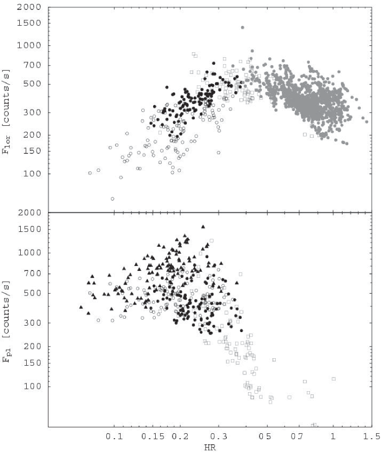
Figure 8: Flux relating to the Lorentzian and power-law components as a function of hardness (9-20 keV over 2-4 keV) under the assumption that the combined fractional RMS of the Lorentzians is constant. The Lorentzian components (upper panel) follow roughly the same hardness-flux pattern as the source in general (compare, e.g., Fig. 7 of Paper I, ). However, the monotonic decrease of $F_{\rm pl}$ (lower panel) with increasing hardness can be explained by the contribution of the power-law decreasing. The true hardness-flux behavior associated with the power-law is positive, and that is why the spread of points appears to systematically decrease. The symbols refer to the different model components used: two Lorentzians (grey points), two Lorentzians and power-law (open squares and black points for transitional and soft state points respectively), Lorentzian plus power-law (open circles) and only power-law (filled triangles).

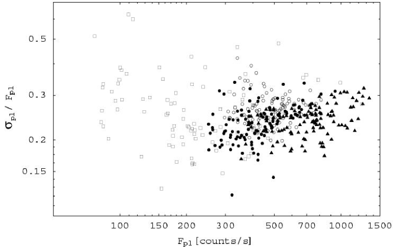
Figure 9: Fractional RMS of the temporal power-law component versus flux related with the component. There is considerable spread, but the result rules out any strong correlation. The symbols are the same as in Fig. 8.

As can be seen by comparing Fig. 8 with the total flux-hardness relation in Cyg X-1 e.g., Fig. 7 in Paper I; Fig. 4 in Zdziarski et al. 2002, it is the behavior of the Lorentzian components that appears to determine the flux-hardness correlation. Furthermore, the flux related with the Lorentzians is reduced in the soft state. The weakening of the Lorentzians in the soft state is thus due to an actual weakening of the corresponding emission component, and not simply due to another emission component growing stronger. The flux related to the power-law component decreases monotonically with increasing hardness. Note however that the spread also increases systematically with flux. As the hardness-flux relation is known to be positive in the soft state (e.g.,  Wen et al. 2001; Zdziarski et al. 2002), it is likely that the general increase in flux is merely a result of the power-law component beginning to dominate the PDS, and that the true hardness-flux relation is positive, and the cause of the systematic increase in spread. The fractional RMS of the power-law (Fig. 9) does not show any strong trend with the associated flux, and the results are consistent with a constant ratio. As seen in the figure, the dispersion is greatest when the power-law component is weak, and decreases as the component becomes stronger. We have calculated the median values in intervals, and they all coincide (within $2\sigma$) with the median when the power-law is the only component seen in the PDS (black triangles in Fig. 9). This value is $0.24\pm 0.004$, and the sample standard deviation is 0.03 (14%).

4 Discussion

In order to establish whether a shift of $L_{1}$ to $L_{1}^{+}$ is truly a possible scenario, all parameters must be examined. We also discuss the results of the PDS decomposition, which provide clues to the relation between the components.

4.1 Shift to first harmonic

If the apparent change in the frequency correlation is caused by $L_{1}$ shifting to a higher harmonic, this should be visible in the other parameter correlations as well. The behavior of $H_{1}$, $W_{1}$ and hardness ratio as a function of fitted Lorentzian frequency does indeed show some clear changes during the transition.

As noted above, the value of the width parameter $W_{1}$ appears to center around 1.2 in the hard state and another, lower value of $\sim 0.7$ in the soft state (panel b in Fig. 3). While this can simply indicate that $L_{1}$ becomes more defined in the soft state, it is interesting to note that a shift to twice the frequency also predicts an increase in the coherence of the signal by a factor of two. While $W_{1}$ is not directly a measure of the coherence, the decrease is consistent with the higher coherence expected if observing $L_{1}$ in the hard state and $L_{1}^{+}$ in the soft state. Our parametrization does not directly give a value for the more generally quoted quality factor $Q=\nu/\Delta\nu$. The relation between $W$ and $Q$ is:

$$W=2\left[1-\left(1+\frac{1}{4Q^{2}}\right)^{-\frac{1}{2}}\right].$$ (9)

Another clue may be obtained when looking at the behavior of $H_{1}$ (panel a in Fig. 3). There is considerable spread in the hard state, but as the source approaches the transition, the value appears to increase slightly, only to decrease sharply as the transition is reached. In the context of a shift to the first harmonic, the rise would start when the strength of $L_{1}^{+}$ becomes comparable to that of $L_{1}$, and the rapid decline is seen when $L_{1}$ begins to weaken. As noted in Sect. 3.2 above, this has to happen fairly rapidly, consistent with the sharp drop in $H_{1}$.

As the hardness is not a parameter of either Lorentzian component, it gives an independent measure of the evolution of the source. It also allows a comparison to determine if the shift in the frequency relation is related to changes in $\nu_{1}$ or $\nu_{2}$ (or both). Plotting the hardness against these two parameters (Fig. 10) does reveal some differences. For $\nu_{2}$, the relation is a smooth power-law, with a flattening at the highest hardness. However, while the $\nu_{1}$ relation also describes a power-law, there is what appears to be a shift during the transition. Though not immediately evident, this shift indicates that the change in the frequency relation is indeed caused by changes in $\nu_{1}$, and is furthermore what would be expected if a shift to the second harmonic occurs.

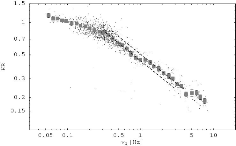
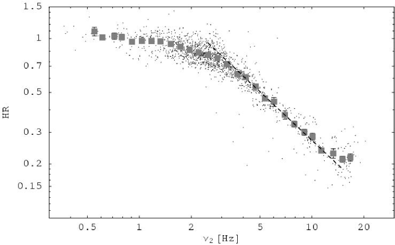
Figure 10: Hardness ratio as a function of $\nu_{1}$ and $\nu_{2}$ respectively. While the relation appears fairly smooth for both components, there is evidence of a shift in the $\nu_{1}$ relation. The filled squares show the results when binning the points along frequency. The dashed lines show the behavior of the $\nu_{i}$-HR relation. For $\nu_{2}$ (lower panel), a single power-law describes the relation through all the states. However, for $\nu_{1}$ it is necessary to shift the power-law during the transition, as seen in the upper panel.

Taken together, the above features provide rather convincing evidence for the idea of a shift from $L_{1}$ to $L_{1}^{+}$ during the transition. The observed properties are certainly consistent with that interpretation. Any suggested model needs to explain all the features consistently, and we find that invoking the shift to $L_{1}^{+}$ is a simple but successful scenario.

We also note that in their long-term study of the PDS of Cyg X-1, Pottschmidt et al. (2003) report a shift in power between their Lorentzian components. In the hard state, the PDS are dominated by $L_{1}$ and $L_{2}$, while during the transitions and ‘failed state transitions’ $L_{1}$ decreases in power and $L_{3}$ strengthens. As their identification of components is not the same as that used here, a direct comparison is not possible. However, the mechanism suggested above is consistent with their results. In addition, results by Pottschmidt et al. (2005) from intermediate state PSD indicate that $L_{1}$ may decrease earlier at higher energies.

An appearance of a QPO with harmonic content has been reported by Belloni et al. (2005) in GX 339-4 in connection with the source shifting from the hard state to the intermediate state. If the change in the frequency relation observed in Cyg X-1 during state transitions is indeed caused by $L_{1}^{+}$ growing in power, the question arises if the appearance of a harmonic is a more general feature of the intermediate state of black hole binaries. The appearance of (or in the case of Cyg X-1, a gradual shift to) a harmonic could then be used as an indicator of spectral state. Certainly the change in the frequency relation may used as a gauge of the state transition in Cyg X-1, and may as such be added to the growing list of possible ways to determine the state of the source. It is likely that all these indicators are responding to the same changes in the source (e.g., accretion geometry) rather than being directly related. Nonetheless, when combined they do provide constraints on proposed models for the state transitions.

In the context of the relativistic precession model discussed in Paper I (Stella & Vietri 1998, 1999; Stella, Vietri, & Morsink 1999) $\nu_{1}=2\nu_{\rm nod}$ and $\nu_{2}=\nu_{\rm per}$, where $\nu_{\rm nod}$ is the frequency of nodal precession and $\nu_{\rm per}$ the frequency of periastron precession. The shift would then mean that $\nu_{1}^{+}=4\nu_{\rm nod}$. Assuming the frequencies are produced close to the inner edge of an accretion disk (or picked out, e.g., from a narrow transition region, see Psaltis & Norman 2000), extending the relation to higher frequencies allows tracking of the disk to smaller radii. Assuming a prograde scenario with dimensionless specific angular momentum $a_{*}=0.49$,

$$\frac{R_{\rm in}}{R_{g}}\simeq 16.5\left(\frac{M}{8\;{\rm M_{\odot}}}\right)^{-\frac{2}{5}}\left(\frac{\nu_{\rm per}}{10\;{\rm Hz}}\right)^{-\frac{2}{5}},$$ (10)

where $R_{\rm in}$ is the inner disk radius, $R_{g}$ the gravitational radius, and $M$ the black hole mass. The dependence on $\left|a_{*}\right|$ is very weak in the studied range.

4.2 Decomposed power spectrum

Although the RMS of the two Lorentzian components show different behaviors and evolution during the hard state, the sum remains constant. While this is no direct evidence that the components are tied, it is improbable that two unrelated components would combine to a constant total. We therefore view the behaviors of the Lorentzians as indicative of them arising from the same physical process. One possibility (especially in the context of the relativistic precession model discussed above) is a scenario where the two components share the same, constant energy. As the amplitude of one grows, the energy available to the other will drop and vice versa.

An extension of this reasoning indicates that the variability giving rise to the power-law component is instead independent of the process behind the Lorentzians. When the power-law enters the frequency window, the total RMS drops, reaching a minimum when the PDS components are all roughly of the same strength. As shown by Zdziarski (2005), this is precisely what is expected if the measured flux arises in different and unrelated processes. We therefore conclude that there are at least two unrelated radiation components producing the PDS of Cyg X-1. One dominates the hard state and provides the variability seen in the Lorentzian components, the other dominates in the soft state and produces the power-law component. The drop in total RMS during transitions can also be seen in Fig. 3 of Pottschmidt et al. (2003).

This scenario fits with previous analyses of the radiation spectrum, which typically include both a soft black-body component and a harder component usually ascribed to Comptonization in a hot corona (e.g., Gierliński et al. 1997, 1999). Recent studies of the energy-dependent variability of Comptonization (Gierliński & Zdziarski 2005) show promising results in tying together temporal and spectral components. Work along these lines has also been presented by Miyamoto et al. (1994) for the source GS~1124-683, and more recently by Vignarca et al. (2003) and Życki & Sobolewska (2005).

An interesting possibility for the two components has been suggested by Ibragimov et al. (2005). They find that the radiation spectrum of the hard state of Cyg X-1 can be well fit using both a thermal and non-thermal distribution of electrons, associated with an inner hot corona and magnetic flares above the accretion disk respectively. The transitions into the soft state can then be explained by the inner edge of the disk moving to smaller radii. As this happens, the corona is reduced (thus weakening the thermal Comptonization component), and emission from the non-thermal distribution connected to the flares becomes more prominent in the radiation spectrum. It is tempting to associate the Lorentzian components with a transition region between the cool disk and the inner quasi-spherical corona, and similarly tying the power-law component of the PDS to emission from a non-thermal distribution of electrons, associated with the flares above the disk. Not only does the relative strength of the power-law increase, but also the cut-off moves to higher frequencies as the source enters the transitional and soft states, when the disk is expected to extend closer to the compact object. Comparing the results of this study with those gained from fitting the radiation spectrum of Cyg X-1 in all states (e.g., Ibragimov et al. 2005; Wilms et al. 2006) indicates that there is no trivial, direct connection between the components of the radiation spectrum and those of the PDS. In order to build a complete physical picture, the behavior of the radio jet of the source also needs to be included. Studies have found correlations between the radio and X-ray flux in Cyg X-1 (e.g., Brocksopp et al. 1999; Pooley et al. 1999), and the radio flux has been connected to the state transitions (Wilms et al. 2006). Furthermore, Migliari et al. (2005) have found correlations between radio luminosity and temporal features of the PDS in a number of X-ray binaries.

If the power-law PDS component is taken to have constant fractional RMS, the value cannot be the same as that for the Lorentzian components. While the distribution in Fig. 9 does not rule out a trend in the fractional RMS, drastic changes are not consistent with the data. We have performed Spearman rank correlation analysis and find only very weak correlations between the parameters of the power-law and those of the Lorentzians. If the power-law component is connected with simple shot noise, the flat behavior seen in Fig. 9 indicates that the increase in flux is due to the amplitude of the shots increasing, and not to a greater number of shots, as that would reduce the observed fractional RMS. The results are consistent with the RMS being proportional to the flux, as shown by Uttley & McHardy (2001).

In a study of the relation between RMS and flux on both longer and shorter timescales, Gleissner et al. (2004) find that the fractional RMS in the $1-32$ Hz frequency band to be constant throughout the hard state changes of PDS, similar to the results presented above. They investigate the RMS-flux correlation in terms of a linear relation and show that such a relation is present in both the hard and soft states of Cyg X-1. However, the slope and intersect of the linear relation have different values in different states. While the paper mainly concentrates on interpretations in terms of a component with either constant flux or constant RMS, the authors also mention the possibility of a component with constant fractional RMS. We find this interpretation to fit well with the results presented in this paper, where both the sum of the Lorentzian components as well as the power-law component display such behavior. As noted above, the two cannot have the same value for a constant fractional RMS, and it is therefore natural that the parameters the RMS-flux relation be different in the hard and soft state, as the power-law is not visible in the former but dominates the latter. During the intermediate state, both components are present, resulting in parameter values in-between the hard and soft state values, as reported by Gleissner et al. (2004).

5 Conclusions

We have conducted an in-depth investigation of the soft and transitional state PDS of Cyg X-1 both reanalyzing previous data and adding data from new soft state observations. Fitting the PDS with a model of two Lorentzian components and cut-off power-law, we are able to extend the frequency relation Wijnands & van der Klis 1999; Paper I into the soft state. We show that the index of the relation is consistent with that found in the hard state. This further supports the identification of the frequencies as the relativistic precessional frequencies.

Using an approach of Monte Carlo simulations we show that a shift in $L_{1}$ from $\nu_{1}$ to its first harmonic $\nu_{1}^{+}=2\nu_{1}$ is consistent with the behavior of all parameters. We conclude that this scenario provides a simple explanation of the observational data.

Combining these results with the hard and transitional state results from Paper I, we decomposed the PDS and studied the evolution of the individual components. The results show that although each Lorentzian is variable, the total fractional RMS is constant throughout the hard state of the source. In contrast, when the power-law component enters the frequency window, the total RMS drops. Together with the lack of correlation between power-law and Lorentzian parameters, this suggests that these components arise in different regions and/or through different processes. Using the observed behavior, we attempted to derive the relation between hardness and flux for the PDS components, as well as the relation between flux and RMS for the power-law. We conclude that the weakening of the Lorentzian components as the source enters the soft state is due to an actual decrease in the associated flux component.

The results show that at least two variability components must be present in the 2-9 keV energy range studied here. In order to better understand both Cyg X-1 and similar objects, studies of both temporal and radiation spectra need to be taken into account. Only by combining the insights from these fields can we hope to understand these sources.