Foreground Subtraction of Cosmic Microwave Background Maps using WI-FIT (Wavelet based hIgh resolution Fitting of Internal Templates)

Abstract

We present a new approach to foreground removal for Cosmic Microwave Background (CMB) maps. Rather than relying on prior knowledge about the foreground components, we first extract the necessary information about them directly from the microwave sky maps by taking differences of temperature maps at different frequencies. These difference maps, which we refer to as internal templates, consist only of linear combinations of galactic foregrounds and noise, with no CMB component. We obtain the foreground cleaned maps by fitting these internal templates to, and subsequently subtracting the appropriately scaled contributions of them from, the CMB dominated channels. The fitting operation is performed in wavelet space, making the analysis feasible at high resolution with only a minor loss of precision. Applying this procedure to the WMAP data, we obtain a power spectrum that matches the spectrum obtained by the WMAP team at the signal dominated scales. The fact that we obtain basically identical results without using any external templates has considerable relevance for future observations of the CMB polarization, where very little is known about the galactic foregrounds. Finally, we have revisited previous claims about a north-south power asymmetry on large angular scales, and confirm that these remain unchanged with this completely different approach to foreground separation. This also holds when fitting the foreground contribution independently to the northern and southern hemisphere indicating that the asymmetry is unlikely to have its origin in different foreground properties of the hemispheres. This conclusion is further strengthened by the lack of any observed frequency dependence.

1 Introduction

The Wilkinson Microwave Anisotropy Probe (WMAP) satellite (Bennett et al., 2003a) and other recent ground-based and balloon-borne experiments have provided high sensitivity observations of the Cosmic Microwave Background (CMB). High-precision estimates of the cosmological parameters have been derived from these data, and these will improve yet further with data from Planck and near-future ground based experiments. Later still, high sensitivity polarization data of the CMB will be available and the physics of the early universe can be studied with even higher fidelity. However, in order to obtain reliable estimates of the cosmological parameters, control of systematic effects and the different sources of foreground contamination is of the utmost importance. In this paper we address the latter problem.

There are three well-understood sources of diffuse galactic contamination. Synchrotron emission from the Galaxy originates in relativistic cosmic ray (CR) electrons spiraling in the Galactic magnetic field. Free-free emission is the bremsstrahlung radiation resulting from the Coulomb interaction between free electrons and ions in the Galaxy. Thermal dust emission arises from grains large enough to be in thermal equilibrium with the interstellar radiation field. Evidence of an additional component initially arose from the cross-correlation of the COBE-DMR data with the DIRBE map of thermal dust emission at 140$\mu$m (Kogut et al., 1996) that revealed anomalous emission with a spectrum rising as the frequency decreased from 53 to 31.5 GHz. Both Banday et al. (2003) and Bennett et al. (2003b) suggested that this component was characterized by a power-law frequency spectrum with index -2.5 over the range $\sim$20 - 60 GHz. However, it remains unclear what the physical origin of such emission is – Bennett et al. (2003b) have proposed that it arises from hard synchrotron emission in star-forming regions close to the Galactic plane, whilst Draine & Lazarian (1998) suggest rotational emission from very small grains or ‘spinning dust’. Recently, Watson et al. (2005) have shown that observations of the Perseus molecular cloud between 11 and 17 GHz and augmented with the WMAP data can be adequately fitted by a spinning dust model. Nevertheless, we will refer to the putative component as anomalous dust.

Fortunately, the foreground components have frequency spectra very different from the CMB, although the exact shapes of these spectra are not known. Most data on galactic emission have been taken at frequencies others than those used for CMB observations and it is not clear whether using these as templates for CMB foreground subtraction is a valid approach. Certainly spatial variations in the frequency dependence of the foregrounds will cause the templates to increasingly diverge from the true structure at microwave wavelengths. Nevertheless, given the lack of other reliable approaches, a template fitting and subtraction procedure was applied on the WMAP data (Bennett et al., 2003a) using external templates (Bennett et al., 2003b; Hinshaw et al., 2003). The Spectral Matching Independent Component Analysis (SMICA) (Delabrouille et al., 2003) method has been applied to the WMAP maps after they had already been cleaned using the standard external templates and evidence for a residual galactic component was found (Patanchon et al., 2005). The WMAP data were also corrected using the Internal Linear Combination (ILC) methods (Bennett et al., 2003b; Tegmark et al., 2003; Eriksen et al., 2004a) but unfortunately these methods are biased (Eriksen et al., 2004a). Other methods that have been developed for foreground subtraction (Barreiro et al., 2004; Hobson et al., 1998; Stolyarov et al., 2002, 2005; Maino et al., 2002, 2003; Donzelli et al., 2005; Brandt et al., 1994; Eriksen et al., 2005) have yet to be applied to the WMAP data.

The importance of being able to make reliable foreground corrections on large angular scales with limited knowledge about the foreground components becomes even more apparent when considering future CMB polarization observations. A very important test of inflation depends on high precision measurements of the predicted B-mode polarization of the CMB on large angular scales. However, very little is known about the polarization of the galactic emission. Future high sensitivity measurements of the CMB polarization are likely to be highly dependent on foreground subtraction methods that do not make strong assumptions about the nature of the galactic emission.

Here we propose a new foreground subtraction method for which no knowledge about the morphology or frequency spectra of galactic components are required. The method does not require constant (in frequency) spectral indexes for the galactic emission components and will therefore not be biased by uncertainties in the changes of the spectral indexes over large frequency ranges. It will however require the spectral indexes to be constant in space over a given patch on the sphere. In the implementation presented here, we assume the spectral indexes to be constant over the full sphere or over hemispheres but the extension to smaller patches will be discussed. As the method increases the noise level in the data, it is at present mainly useful for studies of the larger scales where noise is not dominant. This is particularly relevant given that the largest angular scales in the WMAP data have indicated the presence of several anomalies, in particular a north-south asymmetry in the power spectrum (Eriksen et al., 2004b; Hansen et al., 2004). This result will be re-examined here with our new foreground corrected map.

The method presented here takes advantage of the fact that the observed data already provide information about the foregrounds. In particular, by computing differences of maps observed at different frequencies, (noisy) linear combinations of the foregrounds components are obtained. Fitting and subtracting such templates that are simple linear combinations of the foregrounds is mathematically equivalent to fitting and subtracting templates of the physical foreground components. The advantage of such linear combinations is that they can be obtained directly from the microwave observations themselves and therefore do not rely on other experiments. As a consequence, the foreground morphologies are likely to be well traced even in the presence of modest departures from a single spectral index in a given region.

In §2, we present basis of the method and demonstrate its application in detail. Then, in §3 and §4 the results of this procedure as applied to both simulated inputs and the WMAP sky maps are presented. Finally, in §5, we discuss how the method can be improved in the future.

2 Methodological Basis: Fitting and Subtracting Internal Templates

A pixelized temperature map of microwave observations can be written (in thermodynamic temperatures) as

$$T_{i}^{\nu}=T_{i}^{\mathrm{CMB}}+n_{i}^{\nu}+\sum_{t=1}^{N_{t}}c_{t}^{\nu}s_{i}^{t}.$$ (1)

Here $T_{i}^{\nu}$ is the observed temperature in pixel $i$ for frequency channel $\nu$, $T_{i}^{\mathrm{CMB}}$ is the frequency independent CMB component, $n_{i}^{\nu}$ is the instrumental noise and finally $s_{i}^{t}$ is the contribution from galactic foreground component $t$ for pixel $i$. We assume a total of $N_{t}$ different foreground components. The coefficients $c_{t}^{\nu}$ give the amplitude of the given foreground component $t$ in channel $\nu$. In this paper we assume spatially constant foreground frequency spectra, as was also assumed by the WMAP team in generating the publicly available foreground cleaned maps. However, as discussed in the conclusions, the method can be extended to take into account variations of spectral indexes across the sky, but implementation of this is deferred to a future publication.

2.1 Internal templates

The WMAP team used external templates obtained from observations at other frequencies as tracers of the foreground components $s_{i}^{t}$. The corresponding coefficients $c_{t}^{\nu}$ were then obtained by a fitting procedure (the details of which are not clear) and the inferred foreground contributions subsequently subtracted from the sky maps. Here, we will not use external templates, but instead take the difference between two frequency channels. In such difference maps, which we call internal templates, the CMB cancels out and the remainder is a linear combination of foreground components plus instrumental noise.

We can write the internal templates $D^{\nu\nu^{\prime}}_{i}$, as

$$D^{\nu\nu^{\prime}}_{i}\equiv T_{i}^{\nu}-T_{i}^{\nu^{\prime}}=\sum_{t=1}^{N_{t}}(c_{t}^{\nu}-c_{t}^{\nu^{\prime}})s_{i}^{t}+\delta n_{i}^{\nu\nu^{\prime}},$$ (2)

where $\delta n_{i}^{\nu\nu^{\prime}}=n_{i}^{\nu}-n_{i}^{\nu^{\prime}}$ is the noise of the internal template. Note that we have assumed the maps $T_{i}^{\nu}$ at all frequencies to have been smoothed to the same resolution.

The natural physical ‘basis’ for the foreground components may be identified with dust, synchrotron and free-free emission. The internal templates are transformations into a new basis consisting of linear combinations of the physical components. Fitting and subtracting foreground components in this new basis is clearly mathematically equivalent to using the ’natural basis’, provided that the number of internal templates is equal to the number of components. Therefore, using the internal templates $D^{\nu\nu^{\prime}}_{i}-\delta n_{i}^{\nu\nu^{\prime}}$ as our new basis, equation (1) can be written as

$$T_{i}^{\nu}=T_{i}^{\mathrm{CMB}}+n_{i}^{\nu}+\sum_{t=1}^{N_{t}}\tilde{c}_{t}^{\nu}(D_{i}^{t}-\delta n^{t}),$$ (3)

where the sum is performed over internal templates $t=\nu\nu^{\prime}$ for $N_{t}$ different combinations of channels.

It is important to note that because the internal templates are noisy, subtracting them from the data will increase the overall noise level of the final map and significantly increase the error bars for power spectrum estimates at the highest multipoles.

2.2 Fitting procedure

When using external templates $\hat{s}_{i}^{t}$ for the different foreground components, the fitting procedure is performed by minimizing the $\chi^{2}$,

$$\chi^{2}=\sum_{ij}\sum_{\nu}(T_{i}^{\nu}-\sum_{t}c_{t}^{\nu}\hat{s}_{i}^{t})C^{-1}_{i,j}(T_{j}^{\nu}-\sum_{t}c_{t}^{\nu}\hat{s}_{j}^{t})$$ (4)

for the coefficients $c_{t}^{\nu}$. Here the sum is performed over pixels $i$ and $j$ as well as channels $\nu$ including only the channels we wish to clean. The correlation matrix is defined by $C_{i,j}=\langle T_{i}T_{j}\rangle-\langle T_{i}\rangle\langle T_{j}\rangle$ which can be obtained by Monte-Carlo simulations assuming a reasonable CMB spectrum. In this paper we use a similar fitting procedure, replacing $\hat{s}_{i}^{t}\rightarrow D_{i}^{t}$. In principle we should have used $D_{i}^{t}-\delta n_{i}^{t}$ (see equation 3), but since the noise is known only in a statistical sense we are forced to use $D_{i}^{t}$ and correct for the resulting noise bias. This bias correction procedure will be described in detail in Appendix A.

In practise, the evaluation of equation (4) is not feasible for high resolutions. The covariance matrix is too large to be stored in a computer and too time consuming to invert. For this reason we adopt a wavelet space implementation of the above procedure. The advantage is that we can neglect pixel-pixel correlations, taking only into account the scale-scale correlations in the correlation matrix without significant loss of precision.

We adopt the wavelet fitting procedure of, e.g., Vielva et al. (2004a) and Hansen et al. (2005) and define the cross-correlation coefficients

$$X^{\nu t}_{S}\equiv\sum_{i}w_{iS}^{\nu}w_{iS}^{t},\ \ \ X^{tt^{\prime}}\equiv\sum_{i}w_{iS}^{t}w_{iS}^{t^{\prime}}.$$ (5)

Here $w_{iS}^{\nu}$ is the wavelet transform of $T_{i}^{\nu}$ for pixel $i$, channel $\nu$ and scale $S$, and $w_{iS}^{t}$ is the wavelet transform of the internal template $D_{i}^{t}$. We use Spherical Mexican Hat wavelets (Martínez-González et al., 2002) which are suitable for both template fitting (Vielva et al., 2004a; Hansen et al., 2005), point source detection (Vielva et al., 2003) and tests of non-Gaussianity (Vielva et al., 2004b; Mukherjee & Wang, 2004; Cabella et al., 2004).

In wavelet space, the $\chi^{2}$ to minimize has the form

$$\chi^{2}=\sum_{\nu T}\sum_{SS^{\prime}}(X_{S}^{\nu T}-\sum_{t}\tilde{c}_{t}^{\nu}X_{S}^{tT})C_{SS^{\prime}}^{-1}(X_{S^{\prime}}^{\nu T}-\sum_{t}\tilde{c}_{t}^{\nu}X_{S^{\prime}}^{tT}),$$ (6)

where the summation runs over all target channels $\nu$, all internal templates (foreground components) $T$ and all wavelet scales $S$ and $S^{\prime}$. The scale-scale correlation matrix $C_{SS^{\prime}}$ is obtained by Monte-Carlo simulations. Minimizing the $\chi^{2}$, the best fit $\tilde{c}_{t}^{\nu}$ are given by a set of equations

$$\sum_{t}\tilde{c}_{t}^{\nu}M_{tf}=B_{f}^{\nu}$$ (7)

for each template $f$ and each frequency $\nu$. Here the matrix $M_{tf}$ is given by

$$M_{tf}=\sum_{T}\sum_{SS^{\prime}}X_{S}^{fT}C_{SS^{\prime}}^{-1}X_{S^{\prime}}^{tT}.$$ (8)

and the vector $B_{f}^{\nu}$ by

$$B_{f}^{\nu}=\sum_{T}\sum_{SS^{\prime}}X_{S}^{fT}C_{SS^{\prime}}^{-1}X_{S^{\prime}}^{\nu T}$$ (9)

An estimate of the error bars on the coefficients $\tilde{c}_{t}^{\nu}$ can be obtained performing Monte-Carlo simulations of CMB, noise and ‘foregrounds’. In these simulations, the internal templates obtained from the data are used as ‘foregrounds’ with the best estimate coefficients obtained from the data. An additional correction to the $X_{S}$ is necessary in this case as described in Appendix A. The error bars obtained in this manner has been shown to agree well with the real error bars.

The wavelet scales to use in the analysis are chosen such that the scale-scale correlation matrix is well conditioned. In order to determine these scales, we adopt the following procedure:

• Use MC simulations to obtain $C_{SS^{\prime}}$ for a large set of scales.

• Define a limit $\alpha$, say, 0.95. Start by the smallest allowed scale $S$ and find the next scale by identifying at which scale the normalized covariance matrix $C_{SS^{\prime}}/\sqrt{C_{SS}C_{S^{\prime}S^{\prime}}}$ has fallen to $\alpha$.

• Repeat the above procedure until the largest scale has been reached. Check whether the final correlation matrix is well conditioned. If not, decrease $\alpha$ and repeat.

As in pixel space, a correction procedure for the noise bias has to be implemented. In Appendix A we will describe this procedure in detail as well as a procedure for estimating the level of the remaining bias.

3 Testing the Method on Simulations

The foreground subtraction procedure described above, which we will call Wavelet based hIgh resolution Fitting of Internal Templates (WI-FIT), has been extensively tested on simulated maps. We generated a set of 500 Monte-Carlo simulations of CMB and noise, using the best-fit WMAP power-law power spectrum and noise properties corresponding to the five WMAP channels. To these simulations, we added contributions from known galactic foregrounds based on specific templates. In particular, for thermal dust we use the template provided by Schlegel et al. (1998) extrapolated in frequency by Finkbeiner et al. (1999), for synchrotron we adopt the 408 MHz sky survey of Haslam et al. (1982), and for the free-free contribution we assume that the emission can be traced by a template of H_α emission (Finkbeiner, 2004). The templates are then scaled to the WMAP frequencies using the weights given in Table 4 of Bennett et al. (2003b). These dust weights effectively include an anomalous dust contribution assuming that the putative emission can also be well traced by the thermal dust template.

In order to validate the wavelet basis of our high resolution analysis, we first make an explicit comparison of the method to a full pixel space foreground subtraction procedure at lower resolution where it remains feasible. The maps were therefore smoothed to a common resolution of $5.5^{\circ}$ and degraded to HEALPix resolution $N_{\mathrm{SIDE}}=32$. Unless otherwise stated, the WMAP Kp2 sky cut was applied in all the analyses presented in this paper. Using the procedure with internal templates as described above, then after including the bias correction we obtained unbiased estimates of the foreground coefficients $\tilde{c}_{t}^{\nu}$ in pixel space. Repeating the same procedure in wavelet space yields approximately $2-3\%$ larger error bars showing that the loss in precision using this approach instead of the full pixel space procedure is small. Therefore, since analysis at higher resolution is in any case unfeasible in pixel space, we adopt the wavelet approach in what follows.

We then attempted to calibrate the efficiency of internal versus external template fitting. The WI-FIT procedure was applied to maps of 1 degree FWHM resolution at $N_{\mathrm{SIDE}}=256$ and compared to wavelet-based fitting of external templates. The results derived using 13 wavelet scales is shown in Fig. 1. The two upper maps show the $1\sigma$ residuals for the external and internal template subtraction method when the internal templates were noise-free. These maps $\sigma_{i}$ were obtained by

$$\sigma_{i}\equiv\sqrt{\langle\delta_{i}^{2}\rangle}\equiv\sqrt{\frac{1}{N_{s}}\sum_{s}(M^{s}_{i}-T_{i}^{s})^{2}},$$

where the sum is performed over all simulations $s$, in total $N_{s}=500$, $M^{s}_{i}$ is the cleaned map for pixel $i$ and realization $s$ and $T_{i}^{s}$ is the input CMB realization.

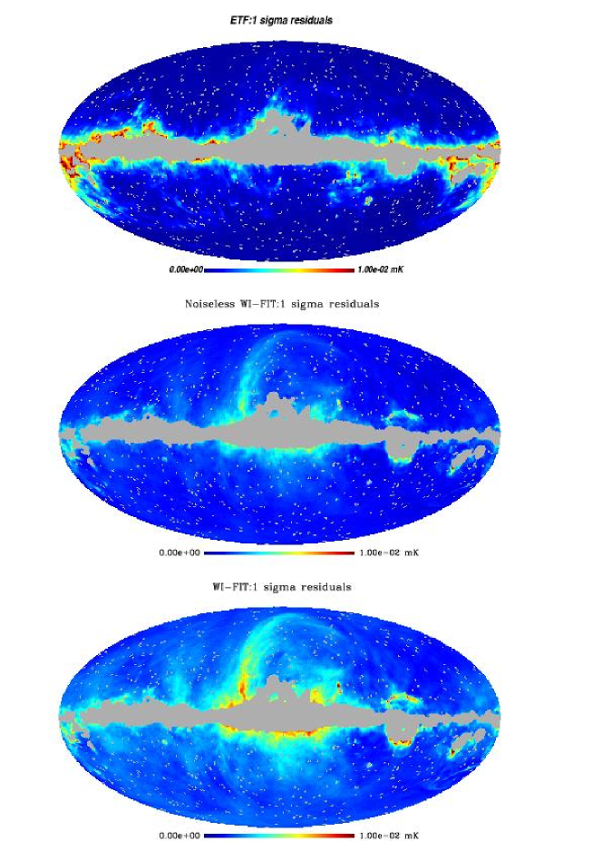
Figure 1: Results from 500 Monte-Carlo simulations: The upper plot shows the $1\sigma$ residuals $\sqrt{\langle\delta_{i}^{2}\rangle}$ on the V-band from the wavelet fitting procedure using external templates. The middle and lower plot show the same result when using internal templates without and with noise respectively. Note that in these simulations the external templates are equal to the foregrounds added to the simulated maps. In reality, templates taken at frequencies different from the ones dominated by the CMB will differ from the foregrounds contaminating the CMB. This additional error is not reflected in the upper plot. Note further that the last case generally has higher noise variance than the two other cases, but the noise variance has not been included in the plots in order to make the foreground residuals clearer.

Unfortunately, the exercise is not particularly revealing, and mostly emphasises that external templates are likely to outperform internal templates when we know that they accurately describe the foregrounds present in the data. In the example shown here, the internal templates do better close to the galactic plane, but worse outside. Additionally, since the internal templates will be noisy, the $1\sigma$ errors will be further inflated as shown in the lower map. Furthermore, the exact level of residuals will in general depend on the choice of internal templates (the specific difference combinations adopted in the analysis) as well as the nature of the foregrounds. In fact, the comparison somewhat violates the philosophy underpinning the WI-FIT method. The external templates are measured at frequencies different from those used for studies of the CMB and are therefore not likely to accurately trace the foregrounds in the CMB dominated channels (although they do by construction in this test). The internal templates however, are linear combinations of the foregrounds at the channels used for CMB studies. The comparison is therefore not completely fair and the results shown in the plot do not adequately reflect a true comparison. We nevertheless present the results for completeness.

4 Application to the WMAP Data

4.1 The maps

We have applied the WI-FIT method to the first-year WMAP data smoothed to 1 degree FWHM at $N_{\mathrm{SIDE}}=256$ and using the Kp2 pixel mask. For each of the WMAP sky maps covering five frequency bands – K, Ka, Q, V and W (when multiple maps are available at the same frequency we take simple averages of the maps after convolution to the 1 degree FWHM beam) – three internal templates were constructed using the four remaining bands. For example, for the Q-band the internal templates K–Ka, Ka–V and V–W were generated, fitted to the Q-band sky map, and subtracted according to the above prescription.

In Fig. 2, we show the cleaned K, Ka, Q, V and W maps. The template coefficients for the K band are so large that the noise level of the resultant cleaned map is too high to be of practical value in any further analysis and will not be considered in what follows. The maps shown can be obtained by combining the different WMAP bands according to the weights given in table 1. In the upper plot of Fig. 9 we also show a noise-weighted combination of the Q, V and W bands. We do not present error bars here as these error bars only are valid when the model (that the spectral indexes of the foregrounds are the same in all directions) is valid. We know that the assumption of spatially constant spectral indexes is wrong and the error bars would hence be misleading.

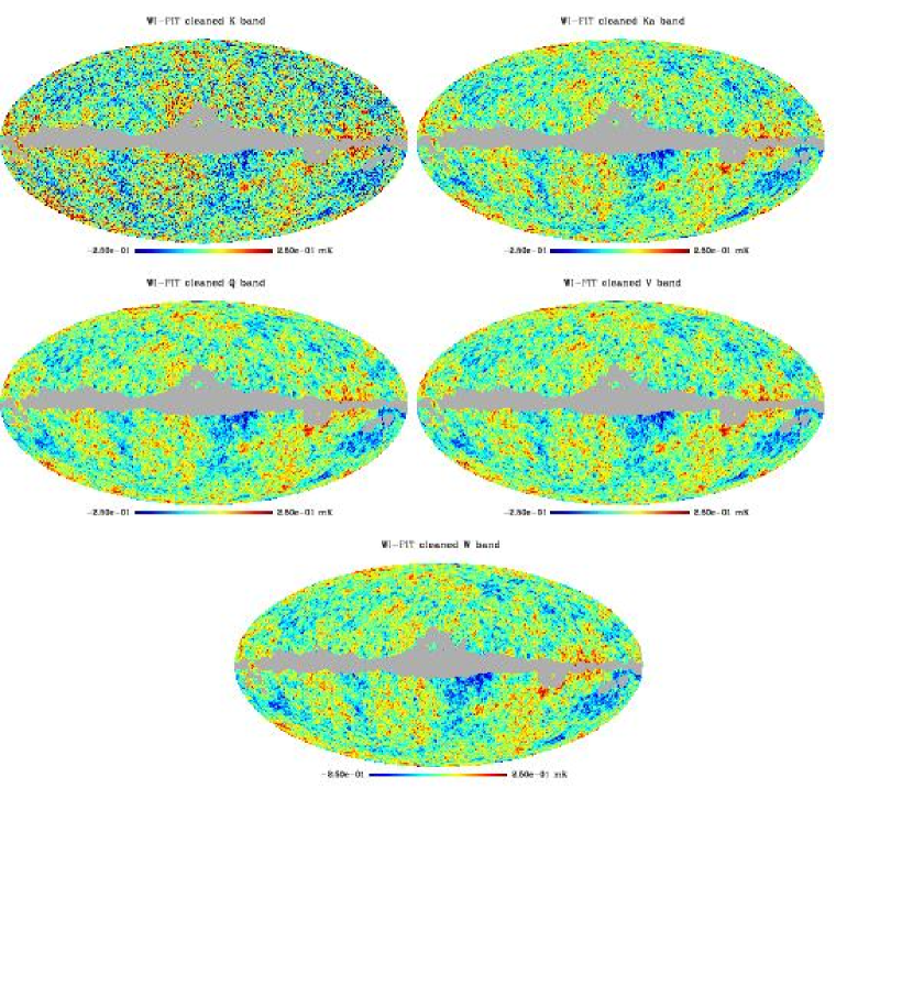
Figure 2: WI-FIT cleaned WMAP maps: The 5 WMAP channels smoothed to a common resolution of 1 degree FWHM and cleaned with the WI-FIT procedure applied outside the Kp2 galactic cut.

In Fig. 2 there are no obvious differences between the Ka, Q, V and W bands. In order to check for possible foreground residuals, we have taken the differences between these sky maps. Since these foreground residuals are generally smaller than the instrumental noise level, the difference maps resemble pure noise without further processing. For visualisation purposes, we have applied a median filter with a 3 degree radius to suppress the noise on pixel scales. Fig. 3 shows the the difference maps for Q–V and V–W. For a perfect foreground subtraction, the difference maps should show little coherent structure beyond that expected for median-filtered pure noise. It is apparent that some small residuals remain outside the Kp2 cut. For comparison, the corresponding differences of the WMAP maps cleaned by External Template Fitting (ETF) provided by the WMAP collaboration are also shown. The ETF maps seem to have stronger residuals than the WI-FIT maps close to the galactic cut. The WI-FIT maps show stronger fluctuations over the whole sky, but this can partly be explained by the higher noise level in these maps.

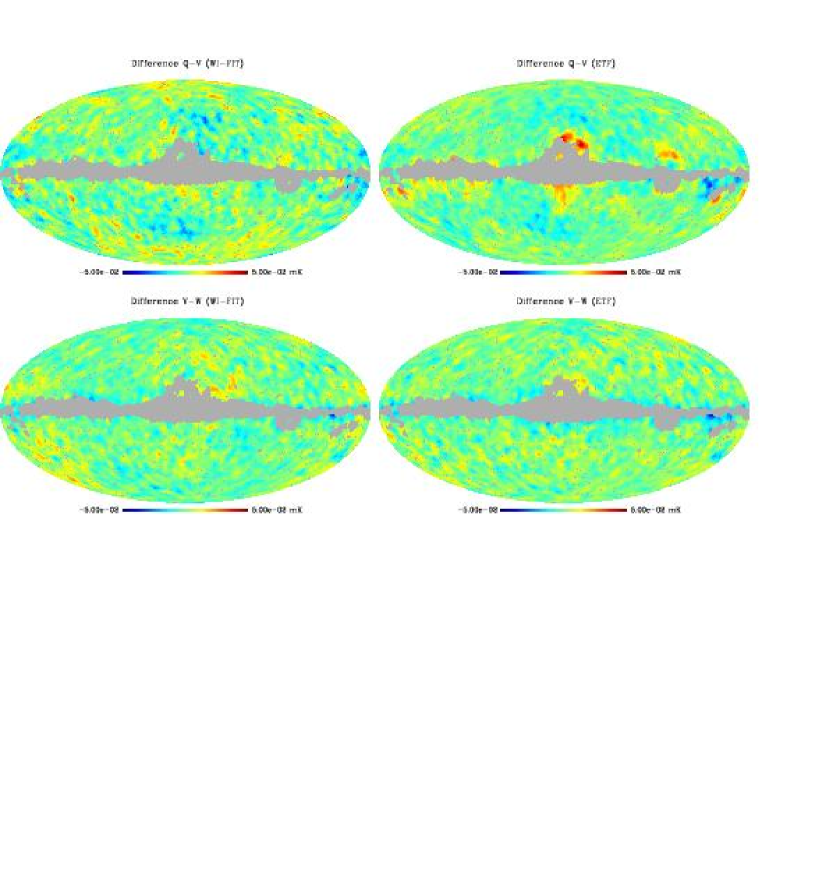
Figure 3: The plots in the left column show the median filtered (3 degree radius top-hat) differences Q-V and V-W for the WI-FIT cleaned WMAP maps where only that part of the sky outside the Kp2 mask was used in the fitting procedure. The plots in the right column show the same differences for the maps that have been foreground corrected by the WMAP collaboration using external templates.

In Figure (4) we show the noise-corrected spectra of these four difference maps. For the Q–V difference, WI-FIT shows stronger residuals in the lowest multipole bin, but ETF has residuals well above $\ell=40$ where the WI-FIT difference spectrum is consistent with pure noise. For the V–W map however, ETF shows stronger residuals in the smallest multipole bin whereas for all other bins the two maps are consistent.

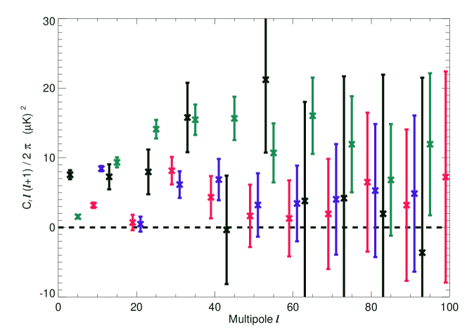
Figure 4: The binned power spectra of the difference maps Q–V and V–W for the ETF and WI-FIT maps (The Kp2 galactic cut was used in the analysis). Black points: WI-FIT Q–V, green points: ETF Q–V, red points: WI-FIT V–W, blue points: ETF V–W. The error bars are obtained from pure noise simulations.

Note further that the Q–V ETF difference map shows strong similarities to the residual component obtained by the SMICA method. Patanchon et al. (2005) found evidence for a residual galactic component (their Figure 5) mainly present in the Q band but not detected in the V band. It is therefore not unexpected that this component shows up when taking the difference Q–V.

In the V–W difference maps one can in both cases see a blue region following the border of the galactic cut (this is more prominent in the ETF maps). As the W band is mainly contaminated by thermal dust, this can be interpreted as a sign of residual thermal dust contamination. That there is a residual thermal dust contamination in the W band is supported by table 1 where we have assumed a spectral index for each foreground component ($\beta_{\mathrm{s}}=-2.7$ for synchrotron, $\beta_{\mathrm{ff}}=-2.15$ for free-free, $\beta_{\mathrm{d}}=2.2$ for thermal dust and $\beta_{\mathrm{sd}}=-2.5$ for anomalous dust) and estimated the proportions of the residual foreground components (see Eriksen et al. (2004a) for details). These numbers indicate the fraction of residual foreground contribution for each type relative to the uncorrected level at an adopted reference frequency (22.8 GHz for synchrotron and anomalous dust, 33.0 GHz for free-free and 93.5 GHz for thermal dust).

In Fig. 5 we show the filtered difference maps between the WI-FIT and ETF maps and the ILC map provided by the WMAP collaboration. The Figures suggest the presence of residuals at the $10\%$ level compared to the CMB over the full sky in either the WI-FIT maps, ETF maps or both. Note that the WMAP-ETF difference for the Q band shows similarities to the residual component detected with SMICA. The fact that the hot and cold areas are interchanged indicates that the residual is not present in the WI-FIT cleaned maps. A ring-like structure on large angular scales is also in all channels. It is not clear whether this residual structure can be attributed to the ETF or the WI-FIT cleaned maps. As the residual is positive in WI-FIT minus ETF, it can either be a strucure which is corrected for in ETF but not in WI-FIT, or an overcorrection in ETF. Looking at the power spectra of these difference maps (Fig. 6), the residual does not significantly affect the estimated CMB power spectra.

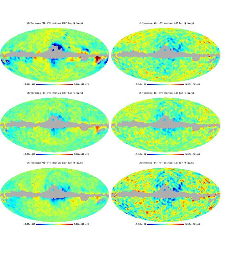
Figure 5: The plot shows the median filtered (3 degree radius top-hat) differences between the WI-FIT and ETF/ILC maps obtained by the WMAP collaboration for the three frequencies Q, V and W.

4.2 The power spectrum

In this section, we consider the implications of these residuals for power spectrum estimation. The MASTER algorithm (Hivon et al., 2002) was applied to the WI-FIT foreground cleaned maps outside the Kp2 sky cut. Before obtaining the spectra, the best fit mono- and dipole were subtracted from all maps. Fig. 6 presents the results (binned version in Fig. 7). For comparison, the power spectrum estimated by the WMAP collaboration (Hinshaw et al., 2003) from the ETF cleaned maps using the cross power spectrum is shown by a solid black line. The WI-FIT spectra are shown as green (Q), blue (V) and red (W) lines and the Ka spectrum is delineated by crosses.

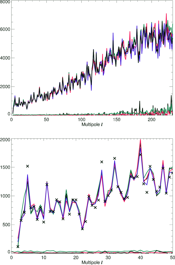
Figure 6: The power spectra of the WI-FIT cleaned WMAP maps for different bands compared to the power spectrum obtained by the WMAP team (solid black line). Green line shows the result for the Q band, blue line for the V band, red line for the W band and black crosses for the Ka band. The lower green and red lines show the power spectra of the difference WI-FIT minus ETF for the Q and W band respectively. The power spectrum of the difference map Q-W for the WI-FIT maps is shown as a black line.

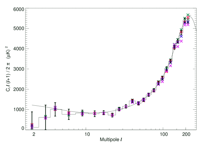
Figure 7: The binned power spectra of the WI-FIT cleaned WMAP maps for different bands compared to the power spectrum obtained by the WMAP team (histogram and error bars). Green crosses show the result for the Q band, blue crosses for the V band, red crosses for the W band and pink crosses for the Ka band.

There is good agreement between the V and W band spectra estimated with the WI-FIT blind approach and the ETF cleaning method based on external observations of the galaxy at very different frequencies. Small differences in the Q band spectrum probably indicate residual foreground contamination, more obviously present in the results for the highly foreground contaminated Ka channel. Nevertheless, both agree reasonably well with the V and W band spectra. Finally, we also show noise-corrected spectra of the WI-FIT and ETF difference maps. The foreground residuals outside the Kp2 cut which show up when taking the difference between the WI-FIT cleaned Q, V and W maps (Fig. 3) as well as the difference between the ETF and WI-FIT maps (Fig. 5) are clearly unlikely to cause significant differences in the CMB power spectrum.

Table 1: WMAP band weights for the WI-FIT cleaned maps and approximate foreground residuals assuming the following spectral indices for the foreground components: $\beta_{\mathrm{synchrotron}}=-2.70$, $\beta_{\mathrm{free-free}}=-2.15$, $\beta_{\mathrm{thermaldust}}=2.20$ and $\beta_{\mathrm{anomalousdust}}=-2.5$. The residuals are given relative to the expected synchrotron and anomalous dust level at 22.8 GHz, free-free level at 33 GHz and thermal dust level at 93.5 GHz.

WMAP band/region	K	Ka	Q	V	W	synch.	ff	th. dust	an. dust
K	1.00	-3.75	0.83	3.81	-0.90	0.04	-0.10	0.42	0.00
Ka	-0.17	1.00	-1.91	2.10	-0.02	-0.06	-0.05	0.52	-0.05
Q	-0.02	-0.75	1.00	0.34	0.44	-0.06	0.05	0.55	-0.05
Q (north)	-0.05	-0.68	1.00	0.50	0.22	-0.06	-0.02	0.44	-0.04
Q (south)	0.46	-2.27	1.00	2.37	-0.57	-0.02	-0.06	0.33	-0.02
V	-0.23	0.66	-0.77	1.00	0.33	-0.07	-0.06	0.55	-0.06
V (north)	-0.33	1.35	-1.55	1.00	0.53	-0.08	-0.06	0.66	-0.06
V (south)	0.21	-1.64	1.35	1.00	0.07	-0.04	-0.06	0.46	-0.04
W	-0.34	0.76	-0.18	-0.24	1.00	-0.10	-0.09	0.75	-0.08
W (north)	-0.62	3.10	-3.49	1.01	1.00	-0.12	-0.14	0.90	-0.10
W (south)	-0.03	-1.45	2.61	-1.13	1.00	-0.08	-0.07	0.66	-0.07
co-added	-0.17	0.06	0.17	0.38	0.56	-0.08	-0.07	0.61	-0.06
co-added (north)	-0.04	-0.64	0.85	0.39	0.43	-0.07	-0.06	0.55	-0.05
co-added (south)	0.20	-1.68	1.54	0.78	0.16	-0.04	-0.05	0.48	-0.04

4.3 Power asymmetries

Eriksen et al. (2004b) and Hansen et al. (2004) reported a significant asymmetry in the distribution of power in the WMAP data. In the reference frame defined by the north pole at $(\theta,\phi)=(80^{\circ},57^{\circ})$ (Galactic co-latitude and longitude), the southern hemisphere was found to have significantly more power on large scales ($\ell<40$) than the northern hemisphere. We therefore re-estimated the power spectra independently in these two hemispheres with the WI-FIT corrected maps, and found remarkably small differences with respect to the previous analyses (see Fig. 8). That these two different approaches to foreground subtraction yield consistent results strengthens the case against an entirely foreground-based explanation of the asymmetry.

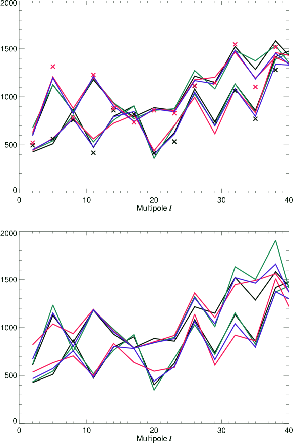
Figure 8: The power spectra taken in the northern (lower lines in each plot) and southern (higher lines in each plot) hemispheres in the frame of reference of maximum asymmetry with the north pole at $(\theta,\phi)=(80^{\circ},57^{\circ})$ in galactic co-latitude and longitude. Solid black lines show the results on the co-added ETF map obtained by the WMAP team. Green line shows the WI-FIT result for the Q band, blue line for the V band, red line for the W band and black crosses for the Ka band. In the upper plot, the results were obtained by applying the WI-FIT fitting procedure on the full sky (outside Kp2). In the lower plot, the fitting procedure was applied separately to the northern hemisphere for the northern spectra and to the southern hemisphere for the southern spectra.

However, one flaw in this argument is that the spectral properties of the foregrounds are assumed to behave uniformly over the sky. We have therefore investigated this issue further by applying the WI-FIT procedure separately to the northern and southern hemispheres. This results in two sets of foreground coefficients, one for each hemisphere, that are subsequently used to generate two different foreground cleaned maps. These are shown in Fig. 9 and the difference channel by channel is shown in Fig. 10. We see that the deviations between the maps can be quite large, even outside the Kp2 cut, supporting the importance of taking into account spatial variations of the spectral index (see the discussion in §5). However, when comparing the northern hemisphere power spectrum corrected by the northern coefficients with the corresponding southern hemisphere corrected by the southern fit, it is evident that a strong asymmetry persists. (lower plot of Fig. 8).

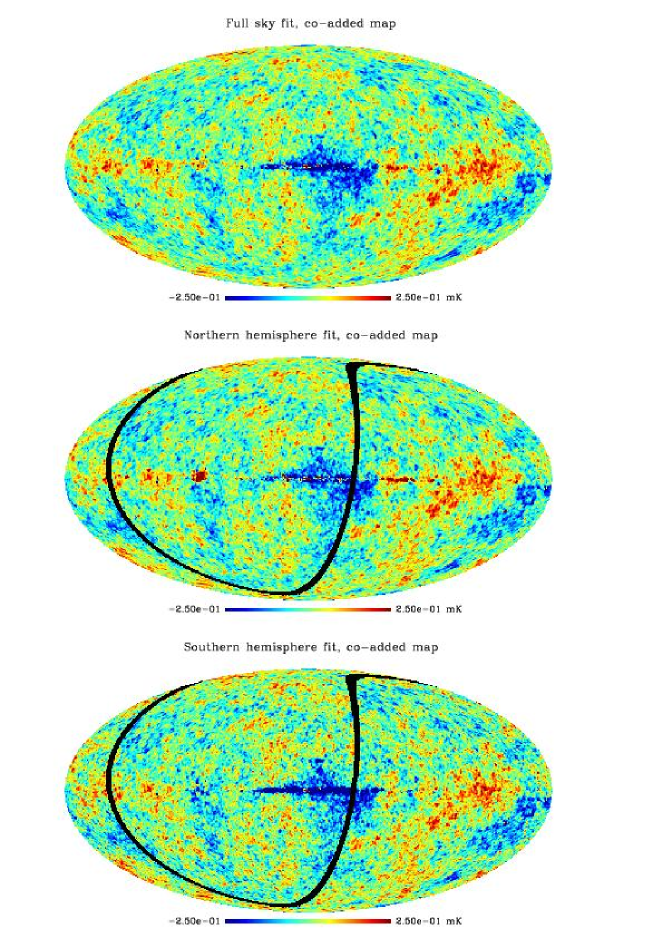
Figure 9: WI-FIT cleaned WMAP maps: the maps have been produced by a noise-weighted combination of the separately cleaned Q, V and W bands. Upper plot shows the result of the fitting procedure applied to the full sky (outside the Kp2 cut), middle/lower plot shows the same map with fitting applied only to the northern/southern (left/right hemisphere on the plot separated by a black band) hemisphere of maximum asymmetry.

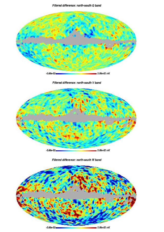
Figure 10: Median filtered (3 degree radius top-hat) differences between the noise-weighted maps obtained by the best fit template coefficients in the north and in the south.

As an additional check, we have applied the ILC method (Eriksen et al., 2004a) to the northern and southern hemisphere separately and derived consistent results. Finally, we evaluated the power spectrum on the northern and southern hemisphere of the map obtained by taking the frequency combination (2.65Ka-K)/1.65, for which synchrotron emission is strongly suppressed. Again, the asymmetry was very similar. If the asymmetry arises as a consequence of residual foregrounds, one would expect it to vary with the foreground subtraction procedure applied. The fact that it does not is a strong argument against a galactic origin for the asymmetry.

5 Discussion and Conclusions

We have introduced a new foreground subtraction method (WI-FIT; Wavelet based hIghresolution Fitting of Internal templates) that uses linear combinations of the foreground components, obtained from the microwave data itself, to fit and subtract foregrounds from the CMB dominated channels. For high resolution maps, the fitting procedure is performed in wavelet space since the pixel space approach is unfeasible for large numbers of pixels. The advantage of this method is that it relies neither on any assumptions nor prior knowledge about the galaxy, nor external observations. All foreground information is obtained from the data themselves by computing differences between maps at different frequencies.

We have demonstrated that the procedure works well on simulated data, based on the experimental parameters of the WMAP satellite. We then applied the method to the WMAP data and obtained a large-scale power spectrum in excellent agreement with that published by the WMAP team (see Fig. 6). We thus obtained the same results without strong constraints on the galactic emission based on external templates. Such a blind analysis method will be of utmost importance for future polarization experiments, for which reliable external templates of polarized galactic components may not be available.

We further showed that the reported power spectrum asymmetry (Eriksen et al., 2004b; Hansen et al., 2004) remains unaltered by this approach to foreground cleaning. This holds true even when the foreground subtraction procedure is applied in the two opposite hemispheres separately. We conclude that the asymmetry is seen at the same level in all frequency bands from $23$ GHz to $94$ GHz and for at least three different foreground subtraction methods. We thus consider the possibility of a galactic origin of the asymmetry as remote.

In the present work, we have assumed that the frequency spectra of the foreground components are independent of position on the sky. This is not a very realistic assumption and also not a necessary one. The WI-FIT method can easily be applied to local regions on the sky individually, although this will likely introduce a more inhomegeneous noise structure to the data. The noisier areas will also need to use more large scale information in order to obtain a sufficiently high signal-to-noise ratio to avoid biased template coefficients, as discussed in Appendix A. The wavelet approach presented is well suited suited for such a scale-dependent procedure.

Finally, we note that the the methods presented here can trivially be extended to polarization maps of Stoke’s parameters Q and U. These issues will be investigated in a future paper.

Appendix A Procedures for noise bias correction and estimation of residual biases

Because of the presence of noise in the internal templates, the template fitting procedure gives biased estimates of the template coefficients. This is easy to see if we take, as an illustration, fitting in pixel space of one noisy template in one channel. Minimizing the $\chi^{2}$ in equation (4), we obtain a best estimate

$$\hat{c}=\frac{\sum_{ij}\hat{s}_{i}C_{ij}^{-1}T_{j}}{\sum_{ij}\hat{s}_{i}C_{ij}^{-1}\hat{s}_{j}}.$$ (A1)

Now we replace the external templates by the noisy internal templates $\hat{s}_{i}\rightarrow D_{i}$ and write the internal templates in terms of a signal part and a noise part as $D_{i}=d_{i}+\delta n_{i}$. We thus obtain

$$\hat{c}=\frac{\sum_{ij}(d_{i}+\delta n_{i})C_{ij}^{-1}T_{j}}{\sum_{ij}(d_{i}+\delta n_{i})C_{ij}^{-1}(d_{j}+\delta n_{j})}=\frac{\sum_{ij}(d_{i}+\delta n_{i})C_{ij}^{-1}(T_{j}^{\mathrm{CMB}}+n_{i}+cd_{i})}{\sum_{ij}(d_{i}+\delta n_{i})C_{ij}^{-1}(d_{j}+\delta n_{j})}.$$ (A2)

Taking the ensemble average, we have

$$\langle\hat{c}\rangle=c\langle\frac{\sum_{ij}(d_{i}+\delta n_{i})C_{ij}^{-1}d_{j}}{\sum_{ij}(d_{i}+\delta n_{i})C_{ij}^{-1}(d_{j}+\delta n_{j})}\rangle,$$ (A3)

where we have used that the CMB and the noise $n_{i}$ in the channel to be cleaned are both uncorrelated with the noise $\delta n_{i}$ in the internal template. We see that when the internal template is noise-free, $\delta n_{i}\rightarrow 0$, the estimate is unbiased $\langle\hat{c}\rangle\rightarrow c$.

We will now go to wavelet space where we will show how this bias factor can be significantly reduced. The bias correction procedure presented in the following can trivially be extended to real space. We will again start with the simplified case of one template and one channel. Then we extend the procedure to the realistic situation and finally we confirm that it works by showing the results from simulated maps.

To simplify notation, we will now write the sum over wavelet scales as

$$X*X\equiv\sum_{SS^{\prime}}X_{S}C_{SS^{\prime}}X_{S^{\prime}}$$ (A4)

Then the best estimate can be written as

$$\hat{c}=\frac{X*X^{\nu}}{X*X},$$ (A5)

where $X_{S}=\sum_{i}(w_{iS}+w_{iS}^{n})^{2}$ and $X_{S}^{\nu}=\sum_{i}(w_{iS}+w_{iS}^{n})w_{iS}^{\nu}$ (see equation 5) where $w_{iS}$, $w_{iS}^{n}$ and $w_{iS}^{\nu}$ are the wavelet transforms of $d_{i}$, $\delta n_{i}$ and $T_{i}^{\nu}$ respectively. Again, the noise term $w_{i}^{n}$ is responsible for the bias and the first step in the bias correction procedure is to remove the noise variance term from $X_{S}$

$$X_{S}\rightarrow X_{S}-\langle(w_{i}^{n})^{2}\rangle=w_{i}^{2}+2w_{i}w_{i}^{n}+\underbrace{(w_{i}^{n})^{2}-\langle(w_{i}^{n})^{2}\rangle}_{\equiv\delta w_{i}^{2}},$$ (A6)

where $\langle(w_{i}^{n})^{2}\rangle$ is obtained from Monte-Carlo simulations of pure noise. The ensemble average is then (see equation A2)

$$\langle\hat{c}\rangle=c\langle\frac{X*(\sum_{i}w_{i}(w_{i}+w_{i}^{n}))}{X*X}\rangle.$$ (A7)

We have noted in simulations that

$$\langle\hat{c}\rangle=\langle\frac{X*X^{\nu}}{X*X}\rangle\approx\frac{\langle X*X^{\nu}\rangle}{\langle X*X\rangle}$$ (A8)

within a few percent accuracy. This suggests that we could correct for the bias if we manage to get the ensemble averages of the numerator and denominator in equation (A7) equal:

$$\langle\hat{c}\rangle\approx c\frac{\langle X*(\sum_{i}w_{i}(w_{i}+w_{i}^{n}))\rangle}{\langle X*X\rangle}\equiv c\frac{\langle N\rangle}{\langle D\rangle}.$$ (A9)

The numerator and denominator can be written as

$$\langle N\rangle=(\sum_{i}w_{i}^{2})*(\sum_{i}w_{i}^{2})+2\langle(\sum_{i}w_{i}w_{i}^{n})*(\sum_{i}w_{i}w_{i}^{n})\rangle$$ (A10)

$$\langle D\rangle=(\sum_{i}w_{i}^{2})*(\sum_{i}w_{i}^{2})+4\langle(\sum_{i}w_{i}w_{i}^{n})*(\sum_{i}w_{i}w_{i}^{n})\rangle+\langle(\sum_{i}\delta w_{i}^{2})*(\sum_{i}\delta w_{i}^{2})\rangle$$ (A11)

Clearly, by subtracting the following terms from the denominator, the average value of the numerator and denominator will become equal and the estimate $\hat{c}$ will become unbiased provided equation (A8) holds. The second step of the bias correction will thus be

$$D\rightarrow D-2\langle(\sum_{i}w_{i}w_{i}^{n})*(\sum_{i}w_{i}w_{i}^{n})\rangle-\langle(\sum_{i}\delta w_{i}^{2})*(\sum_{i}\delta w_{i}^{2})\rangle$$ (A12)

The last term can be easily obtained from Monte-Carlo simulations of pure noise. The first correction term can be obtained from simulations of noise realizations cross-correlated with the internal template $w_{i}+w_{i}^{n}$ taken from the data. Clearly how successful the bias correction is depends on the condition given in equation (A8) and a check of the remaining level of bias would be of high importance. Looking at expression (A7) it is clear that the exact expression for the bias is given by

$$\frac{\hat{c}}{c}=\langle\frac{X*(\sum_{i}w_{i}(w_{i}+w_{i}^{n}))}{X*X}\rangle.$$ (A13)

The problem of obtaining the bias this way is that the noise-free template $w_{i}$ is unknown. We can however make the approximation that our noisy template is a noise-free foreground and then add noise realizations using Monte-Carlo simulations

$$\hat{b}=\langle\frac{X^{\prime}*(X^{\nu})^{\prime}}{X^{\prime}*X^{\prime}}\rangle,$$ (A14)

where $X^{\prime}=\sum_{i}(w^{\prime}_{i}+w_{i}^{N})^{2}-2\langle(\sum_{i}w_{i}^{n})*(\sum_{i}w_{i}^{n})\rangle$, $(X^{\nu})^{\prime}=w^{\prime}_{i}(w^{\prime}_{i}+w_{i}^{N})-\langle(\sum_{i}w_{i}^{n})*(\sum_{i}w_{i}^{n})\rangle$, $w^{\prime}_{i}=w_{i}+w_{i}^{n}$ is the noisy template obtained from the data and $w_{i}^{N}$ are Monte-Carlo noise realizations. To correct for the fact that the templates $w_{i}$ and $w^{\prime}_{i}$ have a slightly different structure (because of the noise $w_{i}^{n}$), we subtract all contributions of $w_{i}^{n}$ to $\langle N\rangle$ and $\langle D\rangle$ by

$$N\rightarrow N-4\langle(\sum_{i}w_{i}w_{i}^{n})*(\sum_{i}w_{i}w_{i}^{n})\rangle-2\langle(\sum_{i}w_{i}^{n}w_{i}^{N})*(\sum_{i}w_{i}^{n}w_{i}^{N})\rangle-\langle(\sum_{i}\delta w_{i}^{2})*(\sum_{i}\delta w_{i}^{2})\rangle,$$ (A15)

$$D\rightarrow D-4\langle(\sum_{i}w_{i}w_{i}^{n})*(\sum_{i}w_{i}w_{i}^{n})\rangle-4\langle(\sum_{i}w_{i}^{n}w_{i}^{N})*(\sum_{i}w_{i}^{n}w_{i}^{N})\rangle-\langle(\sum_{i}\delta w_{i}^{2})*(\sum_{i}\delta w_{i}^{2})\rangle,$$ (A16)

obtained with Monte-Carlo simulations in the same manner as above. We will later show how the bias obtained in this way compares with the real bias in simulations.

The bias correction procedure described above can easily be extended to the case with several templates and channels. Instead of making corrections to the denominator, corrections are made to the matrix $M_{tf}$ described in section §2. Using the same arguments as above, we find that the corresponding bias correction is given by

$$M_{tf}\rightarrow M_{tf}-M_{tf}^{1}-M_{tf}^{2}-M_{tf}^{nn},$$ (A17)

and the estimate of the remaining bias is obtained in the same manner as above, but again correcting for the additional noise term by

$$M_{tf}\rightarrow M_{tf}-M_{tf}^{n1}-M_{tf}^{n2}-M_{tf}^{n3}-M_{tf}^{n4}-M_{tf}^{1}-M_{tf}^{2}-M_{tf}^{3}-M_{tf}^{4}-M_{tf}^{nn},$$ (A18)

and

$$B_{f}^{\nu}\rightarrow B_{f}^{\nu}-\sum_{t}(M_{tf}^{n3}+M_{tf}^{n4}+M_{tf}^{1}+M_{tf}^{2}+M_{tf}^{3}+M_{tf}^{4}+M_{tf}^{nn}),$$ (A19)

where

$$M_{tf}^{1} = \langle\sum_{T}(\sum_{i}(w_{i}(T)+w_{i}^{n}(T))w_{i}^{N}(t))*(\sum_{i}(w_{i}(T)+w_{i}^{n}(T))w_{i}^{N}(f))\rangle$$ (A20)

$$M_{tf}^{2} = \langle\sum_{T}(\sum_{i}(w_{i}(T)+w_{i}^{n}(T))w_{i}^{N}(t))*(\sum_{i}(w_{i}(f)+w_{i}^{n}(f))w_{i}^{N}(T))\rangle$$ (A21)

$$M_{tf}^{3} = \langle\sum_{T}(\sum_{i}(w_{i}(t)+w_{i}^{n}(t))w_{i}^{N}(T))*(\sum_{i}(w_{i}(T)+w_{i}^{n}(T))w_{i}^{N}(f))\rangle$$ (A22)

$$M_{tf}^{4} = \langle\sum_{T}(\sum_{i}(w_{i}(t)+w_{i}^{n}(t))w_{i}^{N}(T))*(\sum_{i}(w_{i}(f)+w_{i}^{n}(f))w_{i}^{N}(T))\rangle$$ (A23)

$$M_{tf}^{nn} = \langle\sum T(\sum_{i}\delta w_{i}(t)\delta w_{i}(T))*(\sum_{i}\delta w_{i}(f)\delta w_{i}(T))\rangle$$ (A24)

The matrices $M_{tf}^{n1}-M_{tf}^{n4}$ are defined similarly to $M_{tf}^{1}-M_{tf}^{4}$, but with $w_{i}\rightarrow 0$ and the $w_{i}^{n}$ are drawn from an independent Monte-Carlo of noise realizations. Note that the $B_{f}^{\nu}$ used for estimating the bias is constructed in the same manner as the numerator in equation (A14).

Finally these procedures were tested on WMAP-like simulations (described in previous sections). In table (2) we show the size of the remaining bias on the template coefficients after applying the bias correction procedure as well as estimating bias with the above method. We see that the bias is kept at the level of a few percent (but may be as large as $15\%$ when considering hemispheres where the signal to noise is lower). Note also that the estimated bias agrees well with the real bias and in all cases is a conservative estimate of the bias. Note that we have not included the results from the W band as one of the internal templates is completely noise dominated (for the parameters used in the simulation) and the matrix $M_{tf}$ becomes unstable.

For the WMAP data, we estimated the remaining template coefficient biases in the full sky fits to be less than $5\%$ relative to the $1\sigma$ error on the coefficients for all bands. In the hemisphere fits, we found the remaining bias to be in the range $5-20\%$ of $1\sigma$. The only exception was for the fit to the northern hemisphere in the W-band for which the bias was estimated to be $45\%$ of $1\sigma$. Note that the lowest wavelet scales are the scales most affected by noise. By exluding the noise dominated scales, the bias factor can be lowered at the cost of larger error bars. For the fit to the northern hemisphere in the W-band, we remade the analysis excluding the 3 first wavelet scales and found that the bias was reduced to a few percent. However, the results obtained with this map is fully consistent with the map obtained by using all scales and we have therefore chosen to include only the results of the latter in this paper.

Table 2: The real and estimated bias on the internal template coefficients obtained in WMAP-like simulations.

WMAP band/region	real bias range	estimated bias range
Q	$\sim 0.1\%$	$\sim 1\%$
V	$\sim 1\%$	$3-4\%$
Q (north)	$\sim 1\%$	$\sim 1\%$
V (north)	$1-4\%$	$2-6\%$
Q (south)	$2-4\%$	$2-4\%$
V (south)	$10-15\%$	$10-20\%$

References

- Banday et al. (2003) Banday, A. J., Dickinson, C., Davies, R. D., Davis, R. J. & Górski, K.M. 2003, MNRAS, 345, 897
- Barreiro et al. (2004) Barreiro, R. B., Hobson, M. P., Banday, A. J., Lasenby, A. N., Stolyarov, V., Vielva, P., & Górski, K. M. 2004, MNRAS, 351, 515
- Bennett et al. (2003a) Bennett, C. L., et al., 2003, ApJS, 148, 1
- Bennett et al. (2003b) Bennett, C. L., et al., 2003, ApJS, 148, 97
- Brandt et al. (1994) Brandt, W. N., Lawrence, C. R., Readhead, A. C. S., Pakianathan, J. N., & Fiola, T. N. 1994, ApJ, 424, 1
- Cabella et al. (2004) Cabella, P., Hansen, F. K., Marinucci, D., Pagano, D. & Vittorio, N. 2004, Phys. Rev. D, 69, 063007
- Delabrouille et al. (2003) Delabrouille, J., Cardoso, J.-F., & Patanchon, G. 2003, MNRAS, 346, 1089
- Donzelli et al. (2005) Donzelli, S., et al. 2005, MNRAS, submitted, astro-ph-0507267
- Draine & Lazarian (1998) Draine, B. T., & Lazarian, A. 1998, ApJ, 494, L19
- Eriksen et al. (2004a) Eriksen, H. K., Banday, A. J., Górski, K. M., & Lilje, P. B. 2004, ApJ, 612, 633
- Eriksen et al. (2005) Eriksen, H. K., et al. 2005, ApJ, in press, astro-ph-0508268
- Eriksen et al. (2004b) Eriksen, H. K., Hansen, F. K., Banday, A. J., Górski, K. M., & Lilje, P. B. 2004, ApJ, 605, 14
- Finkbeiner (2004) Finkbeiner, D. P. 2004, ApJ, 614, 186
- Finkbeiner et al. (1999) Finkbeiner, D. P., Davis, M., & Schlegel, D. J. 1999, ApJ, 524, 867
- Górski et al. (2005) Górski, K. M., Hivon, E., Banday, A. J.,Wandelt, B. D., Hansen, F. K., Reinecke, M., Bartelman, M. 2005, ApJ, 622, 759
- Hansen et al. (2004) Hansen, F. K., Banday, A. J., & Górski, K. M. 2004, MNRAS, 354, 641
- Hansen et al. (2005) Hansen, F. K., Branchini, E., Mazzotta, P., Cabella, P., & Dolag, K. 2005, MNRAS, 361,753
- Haslam et al. (1982) Haslam, C. G. T., Salter, C. J., Stoffel, H., & Wilson, W. 1982, A&AS,47, 1
- Hinshaw et al. (2003) Hinshaw, G., et al. 2003, ApJS, 148, 135
- Hivon et al. (2002) Hivon, E., Górski, K. M., Netterfield, C. B., Crill, B. P., Prunet, S., Hansen, F. K. 2002, ApJ, 567, 2
- Hobson et al. (1998) Hobson, M. P., Jones, A. W., Lasenby, A. N., & Bouchet, F. R. 1998, MNRAS, 300, 1
- Kogut et al. (1996) Kogut, A., Banday, A. J., Bennett, C. L., Gorski, K. M., Hinshaw, G., & Reach, W. T. 1996, ApJ, 460, 1 Hinshaw, G.; Reach, W. T.
- Maino et al. (2002) Maino, D., et al. 2002, MNRAS, 334, 53
- Maino et al. (2003) Maino, D., Banday, A. J., Baccigalupi, C., Perrotta, F., & Górski, K. M. 2004, MNRAS, 344, 544
- Martínez-González et al. (2002) Martínez-González, E., Gallegos, J. E., Argeso, F., Cayón, L., & Sanz, J. L. 2002, MNRAS, 336, 22
- Mukherjee & Wang (2004) Mukherjee, P. & Wang, Y. 2004, ApJ, 613, 51
- Patanchon et al. (2005) Patanchon, G., Cardoso, J.-F., Delabrouille, J., & Vielva, P. 2005, MNRAS, 364, 1185
- Schlegel et al. (1998) Schlegel, D. J., Finkbeiner, D. P., Davis, M., 1998, ApJ, 500, 525
- Stolyarov et al. (2002) Stolyarov, V., Hobson, M. P., Ashdown, M. A. J., & Lasenby, A. N. 2002, MNRAS, 336, 97
- Stolyarov et al. (2005) Stolyarov, V., Hobson, M. P., Lasenby, A. N., & Barreiro, R. B. 2005, MNRAS, 357, 145
- Tegmark et al. (2003) Tegmark, M., de Oliveira-Costa, A., & Hamilton, A. J. 2003, Phys. Rev. D, 68, 123523
- Vielva et al. (2003) Vielva P., Martínez-González E., Gallegos J. E., Toffolatti L. & Sanz J. L. 2003, MNRAS, 344, 89
- Vielva et al. (2004a) Vielva, P., Martínez-González, E., & Tucci, M. 2004a, MNRAS, in press, preprint, astro-ph-0408252
- Vielva et al. (2004b) Vielva, P., Martinez-Gonzalez, E. , Barreiro, R. B., Sanz, J. L., & Cayon, L. 2004b, ApJ, 609, 22
- Watson et al. (2005) Watson, R.A., et al. 2005, ApJ, 624, 89