An $f(R)$ gravitation for galactic environments

Abstract

We propose an action-based $f(R)$ modification of Einstein’s gravity that admits a modified Schwarzschild-deSitter metric. In the weak field limit this amounts to adding a small logarithmic correction to the newtonian potential. A test star moving in such a spacetime acquires a constant asymptotic speed at large distances. This speed, calibrated empirically, is proportional to the fourth root of the mass of the central body in compliance with the Tully-Fisher relation. A variance of MOND’s gravity emerges as an inevitable consequence of the proposed formalism. It has also been shown (Mendoza et al. 2006) that a) the gravitational waves in this spacetime propagate with the speed of light in vacuum and b) there is a lensing effect added to what one finds in the classic GR.

1 Introduction

Convinced of cosmic speed up and not finding the dark energy hypotheses a compelling explanation, some cosmologists have looked for alternatives to Einstein’s gravitation (Deffayet et al. 2002; Freese et al. 2002; Ahmed et al. 2002; Dvali et al. 2003; Capozziello et al. 2003; Carroll et al. 2003; Norjiri et al. 2003, 2004, and 2006; Das et al. 2005; Sotiriou 2005; Woodard 2006). There is a parallel situation in galactic studies. Dark matter hypotheses, intended to explain the flat rotation curves of spirals or the large velocity dispersions in ellipticals, have raised more questions than answers.

Alternatives to newtonian dynamics have been proposed but have had their own critics. Foremost among such theories, the Modified Newtonian Dynamics (MOND) of Milgrom (1983 a,b,c) is able to explain the flat rotation curves (Sandres et al. 1998 and 2002) and justify the Tully-Fisher relation with considerable success. But it is often criticized for the lack of an axiomatic foundation; see, however, Bekenstein’s (2004) TeVeS theory where he attempts to provide such a foundation by introducing a tensor, a vector, and a scalar field into the field equations of GR.

Here we are concerned with galactic problems. We suggest following cosmologists and look for a modified Einstein gravity tailored to galactic environments. In Sects. 2 and 3 we design an action integral, different but close to that of Einstein-Hilbert, and find a spherically symmetric static solution to it. In Sect. 4 we analyze the orbits of test objects moving in this modified spacetime and demonstrate the kinship of the obtained dynamics with MOND. Section 5 is devoted to concluding remarks.

2 A modified field equation

The model we consider is an isolated mass point. As an alternative to the Einstein-Hilbert action, we assume

$$S=\frac{1}{2}\int f(R)\sqrt{-g}d^{4}x,$$ (1)

where $R$ is the Ricci scalar and $f(R)$ an as yet unspecified, but differentiable function of $R$. Variations in $S$ with respect to the metric tensor lead to the following field equation (Capozziello et al. 2003):

$$R_{\mu\nu}-\frac{1}{2}g_{\mu\nu}\frac{f}{h}=\left(h_{;\mu\nu}-{h_{;_{\lambda}}}^{\lambda}g_{\mu\nu}\right)\frac{1}{h},$$ (2)

where $h=df/dR$. The case $f(R)=R+constant$ and $h=1$ gives the Einstein field equation with a cosmological constant included in it. For the purpose of galactic studies, we envisage a spherically symmetric static Schwarzschild-like metric,

$$ds^{2}=-B(r)dt^{2}+A(r)dr^{2}+r^{2}\left(d\theta^{2}+\sin^{2}\theta d\varphi^{2}\right).$$ (3)

From Eqs. (2) and (3) one obtains

$$\frac{B^{\prime}}{B}+\frac{A^{\prime}}{A}=-r\frac{h^{\prime\prime}}{h}+\frac{1}{2}r\left(\frac{B^{\prime}}{B}+\frac{A^{\prime}}{A}\right)\frac{h^{\prime}}{h},$$ (4)

(5)

$$\frac{B^{\prime\prime}}{B}-\frac{1}{2}\left(\frac{B^{\prime}}{B}+\frac{2}{r}\right)\left(\frac{B^{\prime}}{B}+\frac{A^{\prime}}{A}\right)-\frac{2}{r^{2}}+\frac{2A}{r^{2}}$$ (6)

$$\hskip 17.07164pt=2\frac{h^{\prime\prime}}{h}-(\frac{A^{\prime}}{A}+\frac{2}{r})\frac{h^{\prime}}{h},$$ (7)

(8)

$$\!\!\!\!\frac{B^{\prime\prime}}{B}-\frac{1}{2}\frac{B^{\prime}}{B}\left(\frac{B^{\prime}}{B}+\frac{A^{\prime}}{A}\right)-\frac{2}{r}\frac{A^{\prime}}{A}$$ (9)

$$\!\!\!\!\hskip 17.07164pt=f\frac{A}{h}-\left(\frac{B^{\prime}}{B}+\frac{4}{r}\right)\frac{h^{\prime}}{h},$$ (10)

(11)

$$R=2\frac{f}{h}-\frac{3}{A}\left[\frac{h^{\prime\prime}}{h}+\left\{\frac{1}{2}\left(\frac{B^{\prime}}{B}-\frac{A^{\prime}}{A}\right)+\frac{2}{h}\right\}\frac{h^{\prime}}{h}\right].$$ (12)

Equation (4) is the combination $R_{tt}/B+R_{rr}/A$, Eq. (6) is $R_{rr}/A-R_{\theta\theta}/r^{2}$, and Eq. (9) is the $rr$-component of the field equation. Finally, Eq. (12) is from the contraction of Eq. (2). In principle, for a given $h$ (or$f$) one should be able to solve the four Eqs. (4)-(12) for the four unknowns, $A$, $B$, $R$, and $f$ (or $h$), as functions of $r$.

3 Solutions of Equations (4)-(7)

We are interested in solutions that differ from those of the classic GR by small amounts. For the classic GR one has $h=1$ and $A(r)B(r)=1$. Here, we argue that, if the combination $B^{\prime}/B+A^{\prime}/A$ is a well-behaved differential expression, it should have a solution of the form $A(r)B(r)=g(r)$. Furthermore, $g(r)$ should differ from 1 only slightly, in order to remain in the vicinity of GR. There are a host of possibilities. For the sake of argument let us assume $g(r)=(r/s)^{\alpha}\approx 1+\alpha\ln(r/s)$, where $\alpha$ is a small dimensionless parameter and $s$ is a length scale of the system to be identified shortly. Equation (4) splits into

$$\frac{B^{\prime}}{B}+\frac{A^{\prime}}{A}=\frac{\alpha}{r},\leavevmode\nobreak\ \leavevmode\nobreak\ \leavevmode\nobreak\ AB=\left(\frac{r}{s}\right)^{\alpha},$$ (13)

$$h^{\prime\prime}-\frac{1}{2}\frac{\alpha}{r}h^{\prime}+\frac{\alpha}{r^{2}}h=0.$$ (14)

Equation (14) has the solution $h=(r/s)^{\beta}$, $\beta=\alpha+O\left(\alpha^{2}\right)$, and $1-\frac{1}{2}\alpha+O\left(\alpha^{2}\right).$ Of these, the solution $h\approx(r/s)^{\alpha}$ satisfies the requirement $h\rightarrow 1$ as $\alpha\rightarrow 0$. The second solution is discarded. Substituting $AB=h=(r/s)^{\alpha}$ in Eq. (6) gives

$$\frac{1}{A}=\frac{1}{(1-\alpha)}\left[1-\left(\frac{s}{r}\right)^{(1-\alpha/2)}+\lambda\left(\frac{r}{s}\right)^{2(1-\alpha/2)}\right],$$ (15)

$$B=\left(\frac{r}{s}\right)^{\alpha}\frac{1}{A},$$ (16)

where $\lambda$ is a constant of integration. Actually there is another constant of integration multiplying the $(s/r)$ term. We have, however, absorbed it in the expression for $s$ that we now define. For $\alpha=0$, Eqs. (15) and (LABEL:e11) are recognized as the Schwarzschild-deSitter metric. Therefore, $s$ is identified with the Schwarzschild radius of a central body, $2GM/c^{2}$, and $\lambda$ with a dimensionless cosmological constant. Substitution of Eqs. (15) and (LABEL:e11) into Eqs. (9) and (12) gives

$$f=\frac{3}{(1-\alpha)}\frac{1}{r^{2}}\left[\alpha\left(\frac{r}{s}\right)^{\alpha}+(2+\alpha)\lambda\left(\frac{r}{s}\right)^{2}\right],$$ (17)

(18)

$$R=\frac{3}{(1-\alpha)}\frac{1}{r^{2}}\left[\alpha+(4-\alpha)\lambda\left(\frac{r}{s}\right)^{(2-\alpha)}\right].$$ (19)

The Ricci scalar of the Schwarzschild space is zero and that of the deSitter or the Schwarzschild-deSitter space is constant. For non zero $\alpha$, however, $R$ is somewhere between these two extremes. At small distances it increases as $r^{-2}$ and at large $r$’s it behaves as $s^{-2}(s/r)^{\alpha}\approx s^{-2}(1-\alpha\ln{r/s})$. The spacetime is asymptotically neither flat nor deSitterian. Cosmologists may find this variable Ricci scalar relevant to their purpose ( see also Brevik et al, 2004, for a different modification of the Schwarzschild-deSitter metric). Likewise, we began with $f$ as a function of $R$ rather than $r$. Elimination of $r$ between Eqs. (17) and (19) provides one in terms of the other. For $\lambda=0$, one easily finds

$$f=(3\alpha)^{\alpha/2}s^{-\alpha}R^{(1-\alpha/2)}\approx R[1-\frac{\alpha}{2}\ln(s^{2}R)+\frac{\alpha}{2}\ln(3\alpha)].$$ (20)

Once more we observe the mild logarithmic correction to the classic GR.

4 Applications to galactic environments

In this section we demonstrate that

• The logarithmic modification of the Einstein-Hilbert action, in the weak field regime, results in a logarithmic correction to the newtonian potential. A test star moving in such a potential acquires a constant asymptotic speed, $v_{\infty}=c\sqrt{\alpha/2}$.

• The asymptotic speed cannot be independent of the central mass. We resort to the observed rotation curves of spirals to find this dependence.

• The high- and low- acceleration limits of the weak-field regime are the same as those of MOND. A kinship with MOND follows.

4.1 Orbits in the spacetime of Equations (15)-(19)

We assume a test star orbiting a central body specified by its Schwarzschild radius, $2GM/c^{2}$. We choose the orbit in the plane $\theta=\pi/2$. The geodesic equations for $r$, $\varphi$, and $t$ are

$$\frac{d^{2}r}{d\tau^{2}}+\frac{1}{2}\frac{A^{\prime}}{A}\left(\frac{dr}{d\tau}\right)^{2}-\frac{r}{A}\left(\frac{d\varphi}{d\tau}\right)^{2}+\frac{1}{2}\frac{B^{\prime}}{A}\left(\frac{dt}{d\tau}\right)^{2}=0,$$ (21)

(22)

$$\left(\frac{d\varphi}{d\tau}\right)^{-1}\frac{d^{2}\varphi}{d\tau^{2}}+\frac{2}{r}\frac{dr}{d\tau}=0,$$ (23)

(24)

$$\left(\frac{dt}{d\tau}\right)^{-1}\frac{d^{2}t}{d\tau^{2}}+\frac{B^{\prime}}{B}\frac{dr}{d\tau}=0,$$ (25)

respectively. Equations (23) and (25) immediately integrate into

$$r^{2}d\varphi/d\tau=J,\leavevmode\nobreak\ \leavevmode\nobreak\ \textrm{a constant},$$ (26)

(27)

$$dt/d\tau=1/B.$$ (28)

Substituting the latter into Eq. (21) and assuming a circular orbit, $dr/d\tau=0$, gives

$$\frac{J^{2}}{r^{3}}=\frac{1}{2}\frac{B^{\prime}}{B^{2}}=\frac{1}{2}\left(\frac{r}{s}\right)^{\alpha}\frac{B^{\prime}}{B^{4}},$$ (29)

where we have used Eq. (LABEL:e11) to eliminate A. In galactic environments what one measures as the circular orbital speed is

$$v=\frac{rd\varphi}{\sqrt{B}dt}=\frac{r}{\sqrt{B}}\frac{d\varphi}{d\tau}\frac{d\tau}{dt}=\frac{\sqrt{B}J}{r}.$$ (30)

Eliminating $J$ between Eqs. (30) and (29) gives

$$v^{2}=\frac{1}{2}\frac{rB^{\prime}}{B}=\frac{1}{2}\left[\alpha-\frac{rA^{\prime}}{A}\right].$$ (31)

Further substitution for $B$ from Eqs. (LABEL:e11) and (15) yields

$$v^{2}=\frac{1}{2}\alpha+\frac{1}{2}\left(1-\alpha/2\right)\frac{\left[\left(\frac{s}{r}\right)^{(1-\alpha/2)}+2\lambda\left(\frac{r}{s}\right)^{2(1-\alpha/2)}\right]}{\left[1-\left(\frac{s}{r}\right)^{(1-\alpha/2)}+\lambda\left(\frac{r}{s}\right)^{2(1-\alpha/2)}\right]}.$$ (32)

To put Eq. (32) in a tractable form:

• We neglect the $\lambda$ term and substitute $s=2GM/c^{2}$.

• We adopt the approximation $x^{-\alpha}=\exp(-\alpha\ln x)=1-\alpha\ln x+O\left(\alpha^{2}\right)$.

• The terms containing $s$ are small. We retain only the first order terms in $s$.

• $v$ is measured in units of $c$. We restore it hereafter.

With these provisions, Eq. (32) reduces to

$$v^{2}=\frac{1}{2}\alpha c^{2}+\frac{GM}{r}\left[1-\frac{1}{2}\alpha\left\{1+\ln\left(\frac{2GM}{c^{2}r}\right)\right\}\right].$$ (33)

A plot of $v^{2}$ as a function of $r$ has the horizontal asymptote $\frac{1}{2}\alpha c^{2}$.

4.2 Determination of $\alpha$

The asymptote in Eq. (33) cannot be a universal constant. It is not possible to imagine that a galaxy and a speck of dust dictate the same speed for distant passing objects. The parameter $\alpha$ should depend on the mass of the gravitating body residing at the origin, because any localized matter will betray no characteristics other than its mass when sensed from far distances. To find the mass dependence of $\alpha$ we resort to observations. From Sanders and Verheijn (1998) and Sanders and McGaugh (2002), we have compiled a list of 31 spirals for which total masses, asymptotic orbital speeds, and velocity curves are reported. The figures in their papers contain the observed circular speeds and the newtonian ones derived from the observed mass of the stellar and HI components of the galaxies. We have selected those objects that a) have a noticeable horizontal asymptote, b) have fairly reduced newtonian speeds by the time the flat asymptote is approached, and c) do not possess anomalously high HI content to hinder estimates of the total mass and the size of the galaxy. We also made the assumption that the total HI and stellar mass are distributed spherically symmetrically and mimic a point mass if observed from far distances. The relevant data along with $\alpha=2v_{\infty}^{2}/c^{2}$ are reported in the table, and the figure is a log-log plot of the calculated $\alpha$ versus the mass. A power law fit to the data gives

$$\alpha=(3.07\pm 0.18)\times 10^{-7}(M/10^{10}M_{\odot})^{0.494}.$$ (34)

It is important to note that Eq. (34) is not a consequence of the present theory, but rather an empirical relation dictated by observations and based on the masses and the asymptotic speeds of a selected list of galaxies reported by Sanders et al. Together with the popularly accepted rule that the masses and the luminosities of spirals are linearly related, it leads to a Tully-Fisher (TF) relation, $Luminosity\propto{v_{\infty}}^{4.05}$. Observational actualities, however, are complicated. In a recent paper, Kregel et al. (2005) distinguish between different TF relations based on the luminosity, disk mass, maximum disk stellar mass, baryonic mass (meaning stellar+HI mass), baryonic + bulge mass, etc. The reported exponents range from $3.23\pm 0.36$ to $4.2\pm 0.23$, depending on the type of qualification; see also Gurovich et al. (2004). A more elaborate discussion of the issue falls beyond the scope of the present paper.

The main sources of error in Eq. (34), both in the exponent and in the slope, are a) the estimates of the total masses of the galaxies, b) the judgment whether what one measures as the asymptotic speed is indeed the orbital speed at the far outskirts of the galaxy, c) the popular assumption that the masses and luminosities of the spirals are linearly related, and finally, d) our heuristic assumption that the galaxies can be treated as spherically symmetric objects. In spite of all these uncertainties, we note that the exponent 0.494 is astonishingly close to 0.5, the figure that one finds from MOND. We also demonstrate in the following section that the slope $3.00\times 10^{-7}$ is in very good agreement with the characteristic acceleration of MOND.

Table 1: The data in the first four columns are from Sanders et al. 2002. The last two columns show the empirical relation between the asymptotic speeds and the masses of the galaxies.

Galaxy	R	M	$v_{\infty}$	$2(v_{\infty}/c)^{2}$	$\alpha_{0}$
	kpc	$10^{10}M_{\odot}$	km/s	$\times 10^{7}$	$\times 10^{12}$
NGC 5533	72.0	22.0	250	13.9	3.02
NGC 3992	30.0	16.22	242	13.0	3.28
NGC 5907	32.0	10.8	214	10.2	3.15
NGC 2998	48.0	11.3	213	10.1	3.05
NGC 801	60.0	12.9	218	10.6	3.00
NGC 5371	40.0	12.5	208	9.61	2.76
NGC 4157	26.0	5.62	185	7.61	3.24
NGC 4217	14.5	4.50	178	7.04	3.35
NGC 4013	27.0	4.84	177	6.96	3.19
NGC 4088	18.8	4.09	173	6.65	3.32
NGC 4100	19.8	4.62	164	5.98	2.81
NGC 3726	28.0	3.24	162	5.83	3.26
NGC 4051	10.6	3.29	159	5.62	3.12
NGC 4138	13.0	3.01	147	4.82	2.80
NGC 2403	19.0	1.57	134	3.99	3.19
UGC 128	40.0	1.48	131	3.81	3.14
NGC 3769	33.0	1.33	122	3.31	2.88
NGC 6503	21.8	1.07	121	3.25	3.14
NGC 4183	18.0	0.93	112	2.79	2.89
UGC 6917	9.0	0.74	110	2.69	3.12
UGC 6930	14.5	0.73	110	2.69	3.14
M 33	9.0	0.61	107	2.54	3.24
UGC 6983	13.8	0.86	107	2.54	2.74
NGC 7793	6.8	0.51	100	2.22	3.10
NGC 300	12.4	0.35	90	1.80	3.02
NGC 5585	12.0	0.37	90	1.80	2.94
NGC 6399	6.8	0.28	88	1.72	3.22
NGC 55	10.0	0.23	86	1.64	3.39
UGC 6667	6.8	0.33	86	1.64	2.83
UGC 6923	4.5	0.24	81	1.46	2.95
UGC 6818	6.0	0.14	73	1.18	3.12

R: radius of the galaxy (kpc); M: stellar + HI mass ($10^{10}M_{\odot}$); $v_{\infty}$: asymptotic speed (km/sec); $\alpha_{0}$: $2(v_{\infty}/c)^{2}M^{-0.494}$.

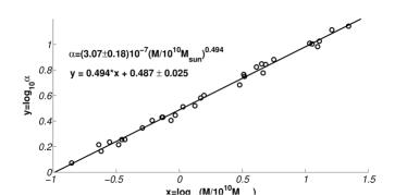
Figure 1: A log-log plot of $\alpha$ versus M. The equation for the power law fit is shown in the legend.

4.3 Kinship with MOND

We recall that in the weak-field approximation, the newtonian dynamics is derived from the Einsteinian one by writing the metric coefficient $B=\left(1+2\phi/c^{2}\right),\phi=GM/r$ and by expanding all relevant functions and equations up to the first order in $\phi/c^{2}$. In a similar way one may find our modified newtonian dynamics from the presently modified GR by expanding $B(r)$ of Eq. (LABEL:e11) up the first order in $\alpha$ and $s/r$. Thus

$$B(r)=1+\alpha+\alpha\ln(r/s)-s/r=1+2\phi(r)/c^{2},$$ (35)

where the second equality defines $\phi(r)$. Let us write Eq. (34) (with slight tolerance) as $\alpha=\alpha_{0}(GM/GM_{\odot})^{1/2}$ and find the gravitational acceleration

$$\leavevmode\nobreak\ \leavevmode\nobreak\ \leavevmode\nobreak\ g \!\!\!\!\leavevmode\nobreak\ = \!\!\!\!\leavevmode\nobreak\ \left|d\phi/dr\right|=(a_{0}g_{n})^{1/2}+g_{n}$$ (36)

$$\!\!\!\!\leavevmode\nobreak\ = \!\!\!\!\leavevmode\nobreak\ g_{n}\leavevmode\nobreak\ \leavevmode\nobreak\ {\rm for}\leavevmode\nobreak\ \leavevmode\nobreak\ g_{n}\gg a_{0}$$

$$\!\!\!\!\leavevmode\nobreak\ = \!\!\!\!\leavevmode\nobreak\ (a_{0}g_{n})^{1/2}\leavevmode\nobreak\ \leavevmode\nobreak\ {\rm for}\leavevmode\nobreak\ \leavevmode\nobreak\ a_{0}\gg g_{n}\rightarrow 0,$$

where we have denoted

$$a_{0}=\alpha_{0}^{2}c^{4}/4GM_{\odot}\leavevmode\nobreak\ \leavevmode\nobreak\ {\rm and}\leavevmode\nobreak\ \leavevmode\nobreak\ g_{n}=GM/r^{2}.$$ (38)

The limiting behaviors of $g$ are the same as those of MOND. One may, therefore, comfortably identify $a_{0}$ as MOND’s characteristic acceleration and calculate $\alpha_{0}$ anew from Eq (38). For $a_{0}=1.2\times 10^{-8}$cm/sec², one finds

$$\alpha=2.8\times 10^{-12}\left(M/M_{\odot}\right)^{1/2}.$$ (39)

It is gratifying how close this value of $\alpha$ is to the one in Eq. (34) and how similar the low and high acceleration limits of MOND and the present formalism are, in spite of their totally different and independent starting points. It should also be noted that there is no counterpart to the interpolating function of MOND here.

5 Concluding remarks

We have developed an $f(R)\propto R^{1-\alpha/2}$ gravitation that is essentially a logarithmic modification of the Einstein-Hilbert action. In spherically-symmetric static situations, the theory allows a modified Schwarzschild-deSitter metric. This metric in the limit of weak fields gives a logarithmic correction to the newtonian potential. From the observed asymptotic speeds and masses of spirals we learn that the correction is proportional to almost the square root of the mass of the central body. Flat rotation curves, the Tully-Fisher relation (admittedly with some reservations), and a version of MOND emerge as natural consequences of the theory.

Actions are ordinarily form invariant under the changes in sources. Mass dependence of $\alpha$ destroys this feature and any claim for the action-based theory should be qualified with such reservation in mind. This, however, should not be surprising, for it is understood that all alternative gravitations, one way or another, go beyond the classic GR. One should not be surprised if some of the commonly accepted notions require re-thinking and generalizations.

Since the appearance of an earlier version of this paper in arXiv, Mendoza et al.(2006) have investigated the gravitational waves and lensing effects in the proposed spacetime. They find the following: a) in any $f(R)=R^{n}$ gravitation, gravitational waves travel with the speed of light in a vacuum, and b) in the present spacetime, there is a lensing in addition to what one finds in the classical GR. Their ratio of the additional deflection angle of a light ray, $\delta\beta$, to that in GR, $\beta_{GR}$, can be reduced to

$$\delta\beta/\beta_{GR}=\frac{1}{2}\alpha\ln{(r_{m}/s-1)},$$ (40)

where $r_{m}$ is the impact parameter of the impinging light. The proportionality of $\delta\beta$ to $\alpha$ is expected, because the proposed metric is in the neighborhood of GR. Its increase with increasing $r_{m}$ also should not be surprising, since the theory is designed to highlight unexpected features at far rather than nearby distances.

Soussa et al. (2004) maintain that “no purely metric-based, relativistic formulation of MOND whose energy functional is stable can be consistent with the observed amount of gravitational lensing from galaxies”. For at least two reasons, this no-go theorem does not apply to what we have highlighted above as the kinship with MOND:

a) Apart from their common low and high acceleration regimes, the two theories are fundamentally different. The gravitational acceleration in the weak field limit of the present theory is the newtonian one to which a small $1/r$ correction is added. That of MOND, on the other hand, is a highly nonlinear function of the newtonian acceleration through an arbitrary interpolating function.

b) More important, however, is one of the authors’ assumptions that “the gravitational force is carried by the metric, and its source is the usual stress tensor”. This is not the case in the present theory. Although we have only worked out the vacuum solution for a point source, the mass dependence of the exponent $\alpha$ in Eqs. (15) and (LABEL:e11) makes the theory different from what the assumption requires.

There are two practices for obtaining the field equations of $f(R)$ gravity, the metric approach, where $g_{\mu\nu}$’s are considered as dynamical variables, and that of Palatini, where the metric and the affine connections are treated as such (see Magnano 1995 for a review). Unless $f(R)$ is linear in $R$, the resulting field equations are not identical (see Ferraris et al. 1994). The metric approach is often avoided for leading to fourth-order differential equations. It is also believed to have instabilities in the weak field approximations (see e. g., Sotiriou 2005 and also Amarzguioui et al. 2005). In the present paper we do not initially specify $f(R)$. Instead, at some intermediate stage in the analysis we adopt an ansatz for $df(R)/dR$ as a function of $r$ and work from there to obtain the metric, the Ricci scalar, and eventually $f(R)$. This enables us to avoid the fourth-order equations. This trick should work in other contexts, such as cosmological ones.

The theory presented here is preliminary. Further investigations are needed from both formal and astrophysical points of view. The author’s list of priorities include the following:

• Stability of the metric of Eqs. (15) &(LABEL:e11). The approach should be to impose a small perturbation $\delta g_{\mu\nu}$ on the metric, linearize the field Eq. (2), and ask for the condition of stability of the metric. Such a condition, if it exists at all, might throw some light on the mass dependence of $\alpha$, the empirical relation of Eq. (39). Managing the linear problems is straightforward. Here, however, the bookkeeping is extensive and laborious.

• Extension of the theory, at least in the weak field regime, to many body systems and to cases with a continuous distribution of matter, in order to obtain the metric inside the matter.

• Developing the theory beyond the first order in $\alpha$

• Solar system tests of the theory.

• Possible cosmological implications of the theory.

Acknowledgement: The author wishes to thank Bahram Mashhoun and Naresh Dadhich for comments and helpful suggestions. Reza Saffari has pointed out a typographical error in the earlier version of the paper, Eq. (15). The error had propagated making the sign of $\alpha$ appear positive in the factor multiplying the term $GM/r$ in Eq. (24). This is corrected here.

References

- (1) Ahmed, M., Dodelson, S., Greene, P. B., & Sorkin, R. 2002, arXiv:astro-ph/0209274
- (2) Amarzguioui, M., Elgaroy, O., Mota, D. F., & Multamaki, T. 2005, arXiv:astro-ph/0510519
- (3) -ibid. 2002, Phys. Rev. D 65, 082004
- (4) Bekenstein, J. D. 2004, arXiv:astro-ph/0403694
- (5) Brevik. I., Norjiri, S., Odintsov, S. D., & Vanzo, L. 2004, Phys. Rev. D, 70, 043520
- (6) Capozziello, S., Cardone, V. F., Carloni, S., & Troisi, A. 2003, arXiv:astro-ph/0307018
- (7) Carroll, S. M., Duvvuri, V., Trodden, M., & Turner, M. S. 2003, arXiv:astro-ph/0306438
- (8) Deffayet, C., Dvali, G. R., & Gabadadze, G. 2002, Phys. Rev. D 65, 044023
- (9) Das, S., Banerjee, N., & Dadhich, N. 2005, arXiv:astro-ph/0505096
- (10) Dvali, G. R., & Turner, M. S. 2001, arXiv:astro-ph/0301510
- (11) Ferraris, M., Francaviglia, M. & Volvich, I. 1994, Class. Quantum Grav. 11, 1505
- (12) Freese, K., & Lewis, M. 2002, Phys. Rev. Lett. B 540, 1
- (13) Gurovich, S., McGaugh, S. S., Freeman, K. C., Jerjen, H., Staveley-Smith, L., & De Blok, W. J. G. 2004, arXiv:astro-ph/0411521
- (14) Kregel, M., van der Kruit, P., C., & Freeman, K. C., arXiv:astro-ph/0501503
- (15) Magnano, G., 1995, arXiv:gr-qc/9511027
- (16) Mendoza, S., & Rosas-Guevara, Y. M., 2006, arXiv:astro-ph/0610390
- (17) Milgrom, M. 1983 a, b & c, 271, 365, 371 & 384
- (18) Norjiri, S., & Odintsov, S. D. 2003, Phys. Rev. D 68, 123512
- (19) -ibid. 2004, GRG 36, 1765
- (20) -ibid. 2006, arXiv:hep-th/0601213
- (21) Sanders, R. H., & Verheijen, M. A. W., 1998, arXiv:astro-ph/9802240
- (22) Sanders, R. H., & McGough, S. S. 2002, arXiv:astro-ph/0204521
- (23) Sotiriou, T. P., 2005, arXiv:gr-qc/0512017
- (24) Soussa, M. E., & Woodard, R. P. 2003, arXiv:astro-ph/0307358
- (25) Woodard, R. P., 2006, arXiv:astro-ph/0601672